Learning All Credible Bayesian Network Structures for Model Averaging

Abstract

A Bayesian network is a widely used probabilistic graphical model with applications in knowledge discovery and prediction. Learning a Bayesian network (BN) from data can be cast as an optimization problem using the well-known score-and-search approach. However, selecting a single model (i.e., the best scoring BN) can be misleading or may not achieve the best possible accuracy. An alternative to committing to a single model is to perform some form of Bayesian or frequentist model averaging, where the space of possible BNs is sampled or enumerated in some fashion. Unfortunately, existing approaches for model averaging either severely restrict the structure of the Bayesian network or have only been shown to scale to networks with fewer than 30 random variables. In this paper, we propose a novel approach to model averaging inspired by performance guarantees in approximation algorithms. Our approach has two primary advantages. First, our approach only considers credible models in that they are optimal or near-optimal in score. Second, our approach is more efficient and scales to significantly larger Bayesian networks than existing approaches.

1 Introduction

A Bayesian network is a widely used probabilistic graphical model with applications in knowledge discovery, explanation, and prediction (Darwiche, 2009; Koller and Friedman, 2009). A Bayesian network (BN) can be learned from data using the well-known score-and-search approach, where a scoring function is used to evaluate the fit of a proposed BN to the data, and the space of directed acyclic graphs (DAGs) is searched for the best-scoring BN. However, selecting a single model (i.e., the best-scoring BN) may not always be the best choice. When one is using BNs for knowledge discovery and explanation with limited data, selecting a single model may be misleading as there may be many other BNs that have scores that are very close to optimal and the posterior probability of even the best-scoring BN is often close to zero. As well, when one is using BNs for prediction, selecting a single model may not achieve the best possible accuracy.

An alternative to committing to a single model is to perform some form of Bayesian or frequentist model averaging  (Claeskens and Hjort, 2008; Hoeting et al., 1999; Koller and Friedman, 2009). In the context of knowledge discovery, Bayesian model averaging allows one to estimate, for example, the posterior probability that an edge is present, rather than just knowing whether the edge is present in the best-scoring network. Previous work has proposed Bayesian and frequentist model averaging approaches to network structure learning that enumerate the space of all possible DAGs (Koivisto and Sood, 2004), sample from the space of all possible DAGs (He et al., 2016; Madigan and Raftery, 1994), consider the space of all DAGs consistent with a given ordering of the random variables (Buntine, 1991; Dash and Cooper, 2004), consider the space of tree-structured or other restricted DAGs (Madigan and Raftery, 1994; Meilă and Jaakkola, 2000), and consider only the $k$-best scoring DAGs for some given value of $k$ (Chen et al., 2015; Chen et al., 2016; Chen et al., 2018; Chen and Tian, 2014; He et al., 2016; Tian et al., 2010). Unfortunately, these existing approaches either severely restrict the structure of the Bayesian network, such as only allowing tree-structured networks or only considering a single ordering, or have only been shown to scale to small Bayesian networks with fewer than 30 random variables.

In this paper, we propose a novel approach to model averaging for BN structure learning that is inspired by performance guarantees in approximation algorithms. Let $\mathit{OPT}$ be the score of the optimal BN and assume without loss of generality that the optimization problem is to find the minimum-score BN. Instead of finding the $k$-best networks for some fixed value of $k$, we propose to find all Bayesian networks $\mathcal{G}$ that are within a factor $\rho$ of optimal; i.e.,

$$\mathit{OPT}\leq\mathit{score}(\mathcal{G})\leq\rho\cdot\mathit{OPT},$$ (1)

for some given value of $\rho\geq 1$, or equivalently,

$$\mathit{OPT}\leq\mathit{score}(\mathcal{G})\leq\mathit{OPT}+\epsilon,$$ (2)

for $\epsilon=(\rho-1)\cdot\mathit{OPT}$. Instead of choosing arbitrary values for $\epsilon$, $\epsilon\geq 0$, we show that for the two scoring functions BIC/MDL and BDeu, a good choice for the value of $\epsilon$ is closely related to the Bayes factor, a model selection criterion summarized in (Kass and Raftery, 1995).

Our approach has two primary advantages. First, our approach only considers credible models in that they are optimal or near-optimal in score. Approaches that enumerate or sample from the space of all possible models consider DAGs with scores that can be far from optimal; for example, for the BIC/MDL scoring function the ratio of worst-scoring to best-scoring network can be four or five orders of magnitude. A similar but more restricted case can be made against the approach which finds the $k$-best networks since there is no a priori way to know how to set the parameter $k$ such that only credible networks are considered. Second, and perhaps most importantly, our approach is significantly more efficient and scales to Bayesian networks with almost 60 random variables. Existing methods for finding the optimal Bayesian network structure (Bartlett and Cussens, 2013; van Beek and Hoffmann, 2015, see e.g.,) rely heavily for their success on a significant body of pruning rules that remove from consideration many candidate parent sets both before and during the search. We show that many of these pruning rules can be naturally generalized to preserve the Bayesian networks that are within a factor of optimal. We modify GOBNILP (Bartlett and Cussens, 2013), a state-of-the-art method for finding an optimal Bayesian network, to implement our generalized pruning rules and to find all near-optimal networks. We show in an experimental evaluation that the modified GOBNILP scales to significantly larger networks without resorting to restricting the structure of the Bayesian networks that are learned.

2 Background

In this section, we briefly review the necessary background in Bayesian networks and scoring functions, and define the Bayesian network structure learning problem (Darwiche, 2009; Koller and Friedman, 2009, for more background on these topics see).

2.1 Bayesian Networks

A Bayesian network (BN) is a probabilistic graphical model that consists of a labeled directed acyclic graph (DAG), $\mathit{G}=(\mathit{V},\mathit{E})$ in which the vertices $\mathit{V}=\{V_{1},\ldots,V_{n}\}$ correspond to $n$ random variables, the edges $E$ represent direct influence of one random variable on another, and each vertex $V_{i}$ is labeled with a conditional probability distribution $P(V_{i}\mid\Pi_{i})$ that specifies the dependence of the variable $V_{i}$ on its set of parents $\Pi_{i}$ in the DAG. A BN can alternatively be viewed as a factorized representation of the joint probability distribution over the random variables and as an encoding of the Markov condition on the nodes; i.e., given its parents, every variable is conditionally independent of its non-descendants.

Each random variable $V_{i}$ has state space $\Omega_{i}$ = $\{v_{i1}$, …, $v_{i{r_{i}}}\}$, where $r_{i}$ is the cardinality of $\Omega_{i}$ and typically $r_{i}\geq 2$. Each $\Pi_{i}$ has state space $\Omega_{\Pi_{i}}=\{\pi_{i1},\ldots,\pi_{i{r_{\Pi_{i}}}}\}$. We use $r_{\Pi_{i}}$ to refer to the number of possible instantiations of the parent set $\Pi_{i}$ of $V_{i}$ (see Figure 1). The set $\theta=\{\theta_{ijk}\}$ for all $i=\{1,\ldots,n\},j=\{1,\ldots,r_{\Pi_{i}}\}$ and $k=\{1,\ldots,r_{i}\}$ represents parameter estimates in $G$ obtained either from expert knowledge or from a dataset, where each $\theta_{ijk}$ estimates the conditional probability $P(V_{i}=v_{ik}\mid\Pi_{i}=\pi_{ij})$.

Figure 1: Example directed acyclic graph of a Bayesian network: Variables $A,B,F$ and $G$ have the state space $\{0,1\}$. The variables $C$ and $E$ have state space $\{0,1,3\}$ and $H$ has state space $\{2,4\}$ Thus $r_{A}=r_{B}=r_{F}=r_{G}=2$, $r_{C}=r_{E}=3$ and $r_{H}=2$. Consider the parent set of $G$, $\Pi_{G}=\{B,C\}$ The state space of $\Pi_{G}$ is $\Omega_{\Pi_{G}}=\{\{0,0\},\{0,1\},\{0,3\},\{1,0\},\{1,1\},\{1,3\}\}.$ and $r_{\Pi_{G}}=6$.

The predominant method for Bayesian network structure learning (BNSL) from data is the score-and-search method. Let $I=\{I_{1},\ldots,I_{N}\}$ be a dataset where each instance $I_{i}$ is an $n$-tuple that is a complete instantiation of the variables in $\mathit{V}$. A scoring function $\sigma(\mathit{G}\mid I)$ assigns a real value measuring the quality of $\mathit{G}=(V_{,}\mathit{E})$ given the data $I$. Without loss of generality, we assume that a lower score represents a better quality network structure and omit $I$ when the data is clear from context.

Definition 1 (credible network).

Given a non-negative constant $\epsilon$ and a dataset $I=\{I_{1},\ldots,I_{N}\}$, a credible network $G$ is a network that has a score $\sigma({\mathit{G}})$ such that $\mathit{OPT}\leq\sigma({\mathit{G}})\leq\mathit{OPT}+\epsilon$, where $\mathit{OPT}$ is the score of the optimal Bayesian network.

In this paper, we focus on solving a problem we call the $\epsilon$-Bayesian Network Structure Learning ($\mathit{\epsilon}\text{BNSL}$). Note that the BNSL for the optimal network(s) is a special case of $\mathit{\epsilon}\text{BNSL}$ where $\epsilon=0$.

Definition 2 ($\mathit{\epsilon}\text{BNSL}$).

Given a non-negative constant $\epsilon$, a dataset $I=\{I_{1},\ldots,I_{N}\}$ over random variables $\mathit{V}$ = $\{V_{1}$, …, $V_{n}\}$ and a scoring function $\sigma$, the $\epsilon$-Bayesian Network Structure Learning ($\mathit{\epsilon}\text{BNSL}$) problem is to find all credible networks.

2.2 Scoring Functions

Scoring functions usually balance goodness of fit to the data with a penalty term for model complexity to avoid overfitting. Common scoring functions include BIC/MDL (Lam and Bacchus, 1994; Schwarz, 1978) and BDeu (Buntine, 1991; Heckerman et al., 1995). An important property of these (and most) scoring functions is decomposability, where the score of the entire network $\sigma(\mathit{G})$ can be rewritten as the sum of local scores associated to each vertex $\sum_{i=1}^{n}\sigma(V_{i},\Pi_{i})$ that only depends on $V_{i}$ and its parent set $\Pi_{i}$ in $\mathit{G}$. The local score is abbreviated below as $\sigma({\Pi_{i}})$ when the local node $V_{i}$ is clear from context. Pruning techniques can be used to reduce the number of candidate parent sets that need to be considered, but in the worst-case the number of candidate parent sets for each variable $V_{i}$ is exponential in $n$, where $n$ is the number of vertices in the DAG.

In this work, we focus on the Bayesian Information Criterion (BIC) and the Bayesian Dirichlet, specifically BDeu, scoring functions. The BIC scoring function in this paper is defined as,

$$BIC:\sigma({\mathit{G}})=-\max_{\theta}L_{G,I}(\theta)+t({G})\cdot w=-\sum_{i=1}^{n}\sum_{j=1}^{r_{\Pi_{i}}}\sum_{k=1}^{r_{i}}n_{ijk}\log\frac{n_{ijk}}{n_{ij}}+\sum_{i=1}^{n}r_{\Pi_{i}}(r_{i}-1)\frac{\log N}{2}.$$

Here, $w=\frac{\log N}{2}$, $t(G)$ is a penalty term and $L_{G,I}(\theta)$ is the log likelihood, given by,

$$L_{G,I}(\theta)=\displaystyle\sum_{i=1}^{n}\sum_{j=1}^{r_{\Pi_{i}}}\sum_{k=1}^{r_{i}}\log\theta_{ijk}^{n_{ijk}},$$

where $n_{ijk}$ is the number of instances in $I$ where $v_{ik}$ and $\pi_{ij}$ co-occur. As the BIC function is decomposable, we can associate a score to $\Pi_{i}$, a candidate parent set of $V_{i}$ as follows,

$$BIC:\sigma({\Pi_{i}})=-\max_{\theta_{i}}L(\theta_{i})+t({\Pi_{i}})\cdot w=-\sum_{j=1}^{r_{\Pi_{i}}}\sum_{k=1}^{r_{i}}n_{ijk}\log\frac{n_{ijk}}{n_{ij}}+r_{\Pi_{i}}(r_{i}-1)\frac{\log N}{2}.$$

Here, $L(\theta_{i})=\sum_{j=1}^{r_{\Pi_{i}}}\sum_{k=1}^{r_{i}}\log\theta_{ijk}^{n_{ijk}}$ and $t(\Pi_{i})=r_{\Pi_{i}}(r_{i}-1)$. The BDeu scoring function in this paper is defined as,

$$BDeu:\sigma({G}) =\displaystyle-\sum_{i=1}^{n}\left(\sum_{j=1}^{r_{\Pi_{i}}}\left(\log\frac{\Gamma\left(\frac{\alpha}{r_{\Pi_{i}}}\right)}{\Gamma\left(\frac{\alpha}{r_{\Pi_{i}}}+n_{ij}\right)}+\sum_{k=1}^{r_{i}}\log\frac{\Gamma\left(\frac{\alpha}{r_{i}r_{\Pi_{i}}}+n_{ijk}\right)}{\Gamma\left(\frac{\alpha}{r_{i}r_{\Pi_{i}}}\right)}\right)\right),$$

where $\alpha$ is the equivalent sample size and $n_{ij}=\sum_{k}n_{ijk}$. As the BDeu function is decomposable, we can associate a score to $\Pi_{i}$, a candidate parent set of $V_{i}$ as follows,

$$BDeu:\sigma({\Pi_{i}}) =\displaystyle-\sum_{j=1}^{r_{\Pi_{i}}}\left(\log\frac{\Gamma\left(\frac{\alpha}{r_{\Pi_{i}}}\right)}{\Gamma\left(\frac{\alpha}{r_{\Pi_{i}}}+n_{ij}\right)}+\sum_{k=1}^{r_{i}}\log\frac{\Gamma\left(\frac{\alpha}{r_{i}r_{\Pi_{i}}}+n_{ijk}\right)}{\Gamma\left(\frac{\alpha}{r_{i}r_{\Pi_{i}}}\right)}\right).$$

3 The Bayes Factor

In this section, we show that a good choice for the value of $\epsilon$ for the $\mathit{\epsilon}\text{BNSL}$ problem is closely related to the Bayes factor (BF), a model selection criterion summarized in (Kass and Raftery, 1995).

The BF was proposed by Jeffreys as an alternative to significance tests (Jeffreys, 1967). It was thoroughly examined as a practical model selection tool in (Kass and Raftery, 1995). Let $\mathit{G}_{0}$ and $\mathit{G}_{1}$ be two DAGs (BNs) in the set of all DAGs $\mathcal{G}$ defined over a set of random variables $V$. The BF in the context of BNs is defined as,

$$BF(\mathit{G}_{0},\mathit{G}_{1})=\frac{P(I\mid\mathit{G}_{0})}{P(I\mid\mathit{G}_{1})},$$

namely the odds of the probability of the data predicted by network $\mathit{G}_{0}$ and $\mathit{G}_{1}$. The actual calculation of the BF often relies on Bayes’ Theorem as follows,

$$\frac{P(\mathit{G}_{0}\mid I)}{P(\mathit{G}_{1}\mid I)}=\frac{P(I\mid\mathit{G}_{0})}{P(I\mid\mathit{G}_{1})}\cdot\frac{P(\mathit{G}_{0})}{P(\mathit{G}_{1})}=\frac{P(I,\mathit{G}_{0})}{P(I,\mathit{G}_{1})}.$$

Since it is typical to assume the prior over models is uniform, the BF can then be obtained using either $P(\mathit{G}\mid I)$ or $P(I,\mathit{G}),\forall\mathit{G}\in\mathcal{G}$. We use those two representations to show how BIC and BDeu scores relate to the BF.

Using the Laplace approximation and other simplifications, Ripley (1996) derived the following approximation to the logarithm of the marginal likelihood for network $\mathit{G}$ (Claeskens and Hjort, 2008, a similar derivation is given in),

$$\log{P(I\mid\mathit{G})}= \max_{\theta}L_{G,I}(\theta)-t({G})\cdot\frac{\log N}{2}+t({G})\cdot\frac{\log{2\pi}}{2}$$

$$-\frac{1}{2}\log{|J_{G,I}(\theta)|}+\log{P(\theta\mid\mathit{G})},$$

where $J_{G,I}(\theta)$ is the Hessian matrix evaluated at the maximum likelihood estimate. It follows that,

$$\log{P(I\mid\mathit{G})}=-BIC(I,\mathit{G})+O(1).$$

The above equation shows that the BIC score was designed to approximate the log marginal likelihood. If we drop the lower-order term, we can then obtain the following equation,

$$BIC(I,\mathit{G}_{1})-BIC(I,\mathit{G}_{0}) =\log{\frac{P(I\mid\mathit{G}_{0})}{P(I\mid\mathit{G}_{1})}}=\log{BF(\mathit{G}_{0},\mathit{G}_{1})}.$$

It has been indicated in (Kass and Raftery, 1995) that as $N\rightarrow\infty$, the difference of the two BIC scores, dubbed the Schwarz criterion, approaches the true value of $\log{BF}$ such that,

$$\frac{BIC(I,\mathit{G}_{1})-BIC(I,\mathit{G}_{0})-\log{BF(\mathit{G}_{0},\mathit{G}_{1})}}{\log{BF(\mathit{G}_{0},\mathit{G}_{1})}}\rightarrow 0.$$

Therefore, the difference of two BIC scores can be used as a rough approximation to $\log{BF}$. Note that some papers define BIC to be twice as large as the BIC defined in this paper, but the above relationship still holds albeit with twice the logarithm of the BF.

Similarly, the difference of the BDeu scores can be expressed in terms of the BF. In fact, the BDeu score is the log marginal likelihood where there are Dirichlet distributions over the parameters (Buntine, 1991; Heckerman et al., 1995); i.e.,

$$\log{P(I,\mathit{G})}=-BDeu(I,\mathit{G}),$$

and thus,

$$BDeu(I,\mathit{G}_{1})-BDeu(I,\mathit{G}_{0}) =\log{\frac{P(I,\mathit{G}_{0})}{P(I,\mathit{G}_{1})}}=\log{BF(\mathit{G}_{0},\mathit{G}_{1})}.$$

The above results are consistent with the observation in (Kass and Raftery, 1995) that the $\log{BF}$ can be interpreted as a measure for the relative success of two models at predicting data, sometimes referred to as the “weight of evidence”, without assuming either model is true. The maximal acceptable distance from the optimal model, however, is often specific to a study and determined with domain knowledge; e.g., a BF of 1000 is more appropriate in forensic science. Heckerman et al. (1995) proposed the following interpreting scale for the BF: a BF of 1 to 3 bears only anecdotal evidence, a BF of 3 to 20 suggests some positive evidence that $\mathit{G}_{0}$ is better, a BF of 20 to 150 suggests strong evidence in favor of $\mathit{G}_{0}$, and a BF greater than 150 indicates very strong evidence. If we deem 20 to be the desired BF in $\mathit{\epsilon}\text{BNSL}$, i.e., $\mathit{G}_{0}=\mathit{G}^{*}$ and $\epsilon=\log(20)$, then any network with a score less than $\log(20)$ away from the optimal score would be credible, otherwise it would be discredited. Note that the ratio of posterior probabilities was defined as $\lambda$ in (Tian et al., 2010; Chen and Tian, 2014) and was used as a metric to assess arbitrary values of $k$ in finding the $k$-best networks.

Finally, the $\mathit{\epsilon}\text{BNSL}$ problem using the BIC or BDeu scoring function given a desired BF can be written as,

$$\mathit{OPT}\leq\mathit{score}(\mathcal{G})\leq\mathit{OPT}+\log{BF}.$$ (3)

4 Pruning Rules for Candidate Parent Sets

To find all near-optimal BNs given a BF, the local score $\sigma(\Pi_{i})$ for each candidate parent set $\Pi_{i}\subseteq 2^{\mathit{V}-\{V_{i}\}}$ and each random variable $V_{i}$ must be considered. As this is very cost prohibitive, it is important that the search space of candidate parent sets be pruned, provided that global optimality constraints are not violated. In this section, we generalize existing pruning rules such that the generalized rules hold when solving the $\mathit{\epsilon}\text{BNSL}$ problem.

A candidate parent set $\Pi_{i}$ can be safely pruned given a non-negative constant $\epsilon\in\mathbb{R}^{+}$ if $\Pi_{i}$ cannot be the parent set of $V_{i}$ in any network in the set of credible networks. Note that for $\epsilon=0$, the set of credible networks just contains the optimal network(s). We discuss the original rules and their generalization below and proofs for each can be found in the appendix.

Teyssier and Koller (2005) give a pruning rule for all decomposable scoring functions. This rule compares the score of a candidate parent set to those of its subsets. We give a relaxed version of the rule.

Lemma 3.

Given a vertex variable $V_{j}$, candidate parent sets $\Pi_{j}$ and $\Pi_{j}^{\prime}$, and some $\epsilon\in\mathbb{R}^{+}$, if $\Pi_{j}\subset\Pi_{j}^{\prime}$ and $\sigma({\Pi_{j}})+\epsilon\geq\sigma({\Pi_{j}^{\prime}})$, $\Pi_{j}^{\prime}$ can be safely pruned if $\sigma$ is a decomposable scoring function.

4.1 Pruning with BIC/MDL Score

A pruning rule comparing the BIC score and penalty associated to a candidate parent set to those of its subsets was introduced in (de Campos and Ji, 2011). The following theorem gives a relaxed version of that rule.

Theorem 4.

Given a vertex variable $V_{j}$, candidate parent sets $\Pi_{j}$ and $\Pi_{j}^{\prime}$, and some $\epsilon\in\mathbb{R}^{+}$, if $\Pi_{j}\subset\Pi_{j}^{\prime}$ and $\sigma({\Pi_{j}})-t({\Pi_{j}^{\prime}})+\epsilon<0$, $\Pi_{j}^{\prime}$ and all supersets of $\Pi_{j}^{\prime}$ can be safely pruned if $\sigma$ is the BIC scoring function.

Another pruning rule for BIC appears in (de Campos and Ji, 2011). This provides a bound on the number of possible instantiations of subsets of a candidate parent set.

Theorem 5.

Given a vertex variable $V_{i}$, and a candidate parent set $\Pi_{i}$ such that $r_{\Pi_{i}}>\frac{N}{w}\frac{\log r_{i}}{r_{i}-1}+\epsilon$ for some $\epsilon\in\mathbb{R}^{+}$, if $\Pi_{i}\subsetneq\Pi_{i}^{\prime}$ , then $\Pi_{i}^{\prime}$ can be safely pruned if $\sigma$ is the BIC scoring function.

The following corollary of Theorem 5 gives a useful upper bound on the size of a candidate parent set.

Corollary 6.

Given a vertex variable $V_{i}$ and candidate parent set $\Pi_{i}$, if $\Pi_{i}$ has more than $\lceil\log_{2}(N+\epsilon)\rceil$ elements, for some $\epsilon\in\mathbb{R}^{+}$, $\Pi_{i}$ can be safely pruned if $\sigma$ is the BIC scoring function.

Corollary 6 provides an upper-bound on the size of parent sets based solely on the dataset size $N$. The following table summarizes such an upper-bound given different amounts of data $N$ and a BF of 20.

$N$	$100$	$500$	$10^{3}$	$5\times 10^{3}$	$10^{4}$	$5\times 10^{4}$	$10^{5}$
$|\Pi|$	7	9	10	13	14	16	17

The entropy of a candidate parent set is also a useful measure for pruning. A pruning rule, given by de Campos et al. (2018), provides an upper bound on the conditional entropy of candidate parent sets and their subsets. We give a relaxed version of their rule. First, we note that the sample estimate of entropy for a variable $V_{i}$ is given by,

$$H(V_{i}) =-\sum^{r_{i}}_{k=1}\frac{n_{ik}}{N}\log\frac{n_{ik}}{N},$$

where $n_{ik}$ represents how many instances in the dataset contain $v_{ik}$, where $v_{ik}$ is an element in the state space $\Omega_{i}$ of $V_{i}$. Similarly, the sample estimate of entropy for a candidate parent set $\Pi_{i}$ is given by,

$$H(\Pi_{i}) =-\sum^{r_{\Pi_{i}}}_{j=1}\frac{n_{ij}}{N}\log\frac{n_{ij}}{N}.$$

Conditional entropy is given by,

$$H(X\mid Y)=H(X\cup Y)-H(Y).$$

Theorem 7.

Given a vertex variable $V_{i}$, and candidate parent set $\Pi_{i}$, let $V_{j}\notin\Pi_{i}$ such that $N\cdot\min\{H(V_{i}\mid\Pi_{i}),H(V_{j}\mid\Pi_{i})\}\geq(1-r_{j})\cdot t(\Pi_{i})+\epsilon$ for some $\epsilon\in\mathbb{R}^{+}$. Then the candidate parent set $\Pi_{i}^{\prime}=\Pi_{i}\cup\{V_{j}\}$ and all its supersets can be safely pruned if $\sigma$ is the BIC scoring function.

4.2 Pruning with BDeu Score

A pruning rule for the BDeu scoring function appears in (de Campos et al., 2018) and a more general version is included in (Correia et al., 2020). Here, we present a relaxed version of the rule in (Correia et al., 2020).

Theorem 8.

Given a vertex variable $V_{i}$ and candidate parent sets $\Pi_{i}$ and $\Pi_{i}^{\prime}$ such that $\Pi_{i}\subset\Pi_{i}^{\prime}$ and $\Pi_{i}\neq\Pi_{i}^{\prime}$, let $r_{i}^{+}(\Pi_{i}^{\prime}):=|\{j:n_{ij}>0,j\in\Omega_{\Pi_{i}^{\prime}}\}|$ be the total number of instantiations of $\Pi_{i}^{\prime}$ that appear in the dataset. If $\sigma({\Pi_{i}})+\epsilon<r_{i}^{+}(\Pi_{i}^{\prime})\log r_{i}$, for some $\epsilon\in\mathbb{R^{+}}$ then $\Pi_{i}^{\prime}$ and the supersets of $\Pi_{i}^{\prime}$ can be safely pruned if $\sigma$ is the BDeu scoring function.

5 Experimental Evaluation

In this section, we evaluate our proposed BF-based method and compare its performance with published $k$-best solvers.

Our proposed method is more memory efficient comparing to the $k$-best based solvers in BDeu scoring and often collects more networks in a shorter period of time. With the pruning rules generalized above, our method can scale up to datasets with 57 variables in BIC scoring, whereas the previous best results are reported on a network of 29 variables using the $k$-best approach with score pruning (Chen et al., 2018).

The datasets are obtained from the UCI Machine Learning Repository (Dheeru and Karra Taniskidou, 2017) and the Bayesian Network Repository. Both BIC/MDL (Schwarz, 1978; Lam and Bacchus, 1994) and BDeu (Buntine, 1991; Heckerman et al., 1995) scoring functions are used where applicable. All experiments are conducted on computers with 2.2 GHz Intel E7-4850V3 processors. Each experiment is limited to 64 GB of memory and 24 hours of CPU time.

We demonstrate the effect of applying pruning rules during scoring in Section 5.1. Our generalized rules are able to eliminate the majority of the search space and therefore allow us to apply the $\epsilon$-BNSL algorithm to medium sized networks. We discuss the implementation details of the BF approach in Section 5.2 and present experimental results with BIC scores on a wide range of datasets commonly used in BNSL. We show the effect of varying sample sizes on our approach using data generated from synthetic BNs in Section 5.3. Finally, We compare our approach with the $k$-best method in Section 5.4.

5.1 The Effect of Pruning

			BIC			BDeu
Data	$n$	$N$	$|\Pi_{3}|$	$|\Pi_{20}|$	$|\Pi_{150}|$	$|\Pi_{20}|$
tic tac toe	10	958	96	110	118	70
wine	14	178	592	949	1,582	1,256
adult	14	32,561	3,660	3,951	4,299	3,686
nltcs	16	3,236	8,287	8,966	9,712	9,074
msnbc	17	58,265	48,043	49,630	51,335	54,280
letter	17	20,000	117,405	120,685	124,133	87,183
voting	17	435	429	497	581	721
zoo	17	101	1,036	1,848	3,419	28,872
hepatitis	20	155	474	1,485	4,437	4,054
parkinsons	23	195	3,212	5,532	10,468	14,415
sensors	25	5456	962,400	1,012,964	1,064,961	OT
autos	26	159	3,413	7,629	17,442	54,511
insurance	27	1,000	530	607	709	OT
horse	28	300	760	2,296	7,361	OT
flag	29	194	1,227	3,888	12,873	OT
wdbc	31	569	17,193	23,923	34,983	OT
mildew	35	1000	128	128	128	OT
soybean	36	266	7,781	14,229	29,691	OT
alarm	37	1000	818	1,588	4,922	OT
bands	39	277	1,422	5,055	19,253	OT
spectf	45	267	1,320	7,407	34,971	OT
sponge	45	76	741	1,267	3,064	OT
barley	48	1000	244	246	256	OT
hailfinder	56	100	185	254	452	OT
hailfinder	56	500	428	459	519	OT
lung cancer	57	32	567	2,392	7,281	OT

Table 1: The number of candidate parents $|\Pi|$ in the pruned scoring file at BF = 3, 20 and 150 using BIC, and at BF = 20 using BDeu, where $n$ is the number of random variables in the dataset, $N$ is the number of instances in the dataset and OT = Out of Time.

We modified the development version (9c9f3e6) of GOBNILP to apply the generalized pruning rules in Section 4. In particular, Lemma 3 is applied to both BIC and BDeu; Theorem 4 and Corollary 6 are applied to BIC; Theorem 8 is applied to BDeu. The combination of those rules effectively pruned more than $95\%$ of the parent sets for almost all datasets. The worst pruning rate of $88.9\%$ is observed on the letter dataset with a BF of 150 using BIC. We report the number of remaining candidate parent sets in Table 1. The generalized pruning rules allow us to scale up to medium sized networks, unlike previous approaches where the lack of effective pruning rules restricts them to small networks.

5.2 The Bayes Factor Approach

Data	$n$	$N$	$T_{3}$ (s)	$|\mathcal{G}_{3}|$	$|\mathcal{M}_{3}|$	$T_{20}$ (s)	$|\mathcal{G}_{20}|$	$|\mathcal{M}_{20}|$	$T_{150}$ (s)	$|\mathcal{G}_{150}|$	$|\mathcal{M}_{150}|$
tic tac toe	10	958	1.9	192	64	2.0	192	64	3.3	544	160
wine	14	178	4.1	308	51	24.9	3,449	576	143.7	26,197	4,497
adult	14	32,561	17.5	324	162	45.1	1,140	570	55.7	2,281	1,137
nltcs	16	3,236	53.8	240	120	201.7	1,200	600	1,005.1	4,606	2,303
msnbc	17	58,265	3,483.0	24	24	7,146.9	960	504	8,821.4	1,938	1,026
letter	17	20,000	OT	—	—	OT	—	—	OT	—	—
voting	17	435	1.3	27	2	4.0	441	33	14.3	2,222	170
zoo	17	101	8.1	49	13	21.9	1,111	270	299.3	21,683	5,392
hepatitis	20	155	7.1	580	105	513.3	87,169	15,358	1,452.8	150,000	49,269
parkinsons	23	195	30.7	1,088	336	3,165.9	150,000	39,720	4,534.3	150,000	116,206
sensors	25	5456	OT	—	—	OT	—	—	OT	—	—
autos	26	159	95.0	560	200	2,382.8	50,374	17,790	6,666.9	150,000	54,579
insurance	27	1,000	49.8	8,226	2,062	244.9	104,870	25,580	414.5	148,925	36,072
horse	28	300	18.8	1,643	246	1,358.8	150,000	28,186	1,962.5	150,000	69,309
flag	29	194	16.1	773	169	4,051.9	150,000	39,428	5,560.9	150,000	122,185
wdbc	31	569	396.1	398	107	10,144.2	28,424	8,182	45,938.2	150,000	54,846
mildew	35	1000	1.2	1,026	2	1.2	1,026	2	2.1	2,052	4
soybean	36	266	7,729.4	150,000	150,000	16,096.8	150,000	62,704	8,893.5	150,000	118,368
alarm	37	1000	6.3	1,508	122	684.2	123,352	9,323	2,258.4	150,000	8,484
bands	39	277	100.9	7,092	810	2,032.6	150,000	44,899	16,974.8	150,000	95,774
spectf	45	267	432.4	27,770	4,510	7,425.2	150,000	51,871	19,664.8	150,000	63,965
sponge	45	76	16.8	1,102	65	1,301.0	146,097	7,905	1,254.4	150,000	90,005
barley	48	1000	0.8	182	1	0.8	364	2	1.3	1,274	5
hailfinder	56	100	171.5	150,000	20	149.4	150,000	748	214.6	150,000	294
hailfinder	56	500	286.1	150,000	30,720	314.1	150,000	18,432	217.3	150,000	24,576
lung cancer	57	32	584.3	150,000	40,621	966.6	150,000	79,680	2,739.7	150,000	48,236

Table 2: The search time $T$, the number of collected networks $|\mathcal{G}|$ and the number of MECs $|\mathcal{M}|$ in the collected networks at BF = 3, 20 and 150 using BIC, where $n$ is the number of random variables in the dataset, $N$ is the number of instances in the dataset and OT = Out of Time.

We modified the development version (9c9f3e6) of GOBNILP, denoted hereafter as GOBNILP_dev, and supplied appropriate parameter settings for collecting near-optimal networks. The code is compiled with SCIP 6.0.0 and CPLEX 12.8.0. GOBNILP extends the SCIP Optimization Suite (Gleixner et al., 2018) by adding a constraint handler for handling the acyclicity constraint for DAGs. If multiple BNs are required GOBNILP_dev just calls SCIP to ask it to collect feasible solutions. In this mode, when SCIP finds a solution, the solution is stored, a constraint is added to render that solution infeasible and the search continues. This differs from (and is much more efficient than) the method used in the current stable version of GOBNILP for finding $k$-best BNs where an entirely new search is started each time a new BN is found. A recent version of SCIP has a separate “reoptimization” method which might allow better $k$-best performance for GOBNILP but we do not explore that here. By default when SCIP is asked to collect solutions it turns off all cutting plane algorithms. This led to very poor GOBNILP performance since GOBNILP relies on cutting plane generation. Therefore, this default setting is overridden in GOBNILP_dev to allow cutting planes when collecting solutions. To find only solutions with objective no worse than ($\mathit{OPT}+\epsilon$), SCIP’s SCIPsetObjlimit function is used. Note that, for efficiency reasons, this is not effected by adding a linear constraint.

Data	$n$	$N$	$T_{k}$ (s)	$k$	$T_{EC}$ (s)	$|\mathcal{G}_{k}|$	$T_{20}$ (s)	$|\mathcal{G}_{20}|$	$|\mathcal{M}_{20}|$
tic tac toe	10	958	0.2	10	0.5	67	0.6	152	24
			2.8	100	6.0	673
			70.7	1,000	78.5	7,604
wine	14	178	3.4	10	12.0	60	35.9	8,734	6,262
			85.0	100	168.4	448
			3,420.4	1,000	3,064.4	4,142
adult	14	32,561	3.3	10	633.5	68	9.3	792	19
			73.6	100	63,328.9	1,340
			2,122.8	1,000	OT	—
nltcs	16	3,236	11.8	10	47,338.4	552	125.5	652	326
			406.6	100	OT	—
			13,224.6	1,000	OT	—
msnbc	17	58,265	ES	—	ES	—	4,018.9	24	24
letter	17	20,000	26.0	10	18,788.0	200	56,344.8	20	10
			909.8	100	OT	—
			41,503.9	1,000	OT	—
voting	17	435	34.1	10	101.9	30	6.0	621	207
			1,125.7	100	1,829.2	3,392
			38,516.2	1,000	42,415.3	3,665
zoo	17	101	33.5	10	99.8	52	8,418.8	29,073	6,761
			1,041.7	100	1,843.4	100
			41,412.1	1,000	OT	—
hepatitis	20	155	351.2	10	872.3	89	441.4	28,024	3,534
			13,560.3	100	20,244.7	842
			OT	1,000	OT	—
parkinsons	23	195	3,908.2	10	OT	—	1,515.9	150,000	42,448
			OT	100	OT	—
			OT	1,000	OT	—
autos	26	159	OM	1	OM	—	OT	—	—
insurance	27	1,000	OM	1	OM	—	8.3	1,081	133

Table 3: The search time $T$ and the number of collected networks $k$, $|\mathcal{G}_{k}|$ and $|\mathcal{G}_{20}|$ for KBest, KbestEC and GOBNILP_dev (BF = 20) using BDeu, where $n$ is the number of random variables in the dataset, $N$ is the number of instances in the dataset, OM = Out of Memory, OT = Out of Time and ES = Error in Scoring. Note that $|\mathcal{G}_{k}|$ is the number of DAGs covered by the $k$-best MECs in KBestEC and $|\mathcal{M}_{20}|$ is the number of MECs in the networks collected by GOBNILP_dev.

We first use GOBNILP_dev to find the optimal score since GOBNILP_dev takes objective limit ($\mathit{OPT}+\epsilon$) for enumerating feasible networks. For BIC, We set the limit on the size of the parent set based on Corollary 6 that guarantees optimality, whereas for BDeu we set the number to $-1$ to allow all possible sizes. Then all networks falling into the limit are collected with a counting limit of 150,000. Finally the collected networks are categorized into Markov equivalence classes (MECs), where two networks belong to the same MEC iff they have the same skeleton and v-structures (Verma and Pearl, 1990). The proposed approach is tested on datasets with up to 57 variables. The search time $T$, the number of collected networks $|\mathcal{G}|$ and the number of MECs $\mathcal{M}$ in the collected networks at BF = 3, 20 and 150 using BIC are reported in Table 2, where $n$ is the number of random variables in the dataset and $N$ is the number of instances in the dataset. The three thresholds are chosen according to the interpreting scale suggested by Heckerman et al. (1995) where 3 marks the transition between anecdotal and positive evidence, 20 marks the transition between positive and strong evidence and 150 marks the transition between strong and very strong evidence. The search time mostly depends on a combined effect of the size of the network, the sample size and the number of MECs at a given BF. Some fairly large networks such as alarm, sponge and barley are solved much faster than smaller networks with a large sample size; e.g., msnbc and letter.

The results also indicate that the number of collected networks and the number of MECs at three BF levels varies substantially across different datasets. In general, datasets with smaller sample sizes tend to have more networks collected at a given BF since near-optimal networks have similar posterior probabilities to the best network. Although the desired level of BF for a study, like the p-value, is often determined with domain knowledge, the proposed approach, given sufficient samples, will produce meaningful results that can be used for further analysis.

5.3 Synthetic Data

We use BNs up to 76 nodes from the Bayesian Network Repository to generate synthetic data in the form of 10 random samples for various sample sizes up to 1,000. Near optimal networks are collected following the same procedure outlined in Section 5.2 using BIC. For the three largest datasets, hailfinder, hepar2, and win95pts, the scoring process failed to complete within 24 hours for the sample size of 1,000.

The average number of networks in the credible sets is reported in Table 4. The results are consistent with Table 2 in demonstrating that the number of collected networks are specific to the dataset. Collecting a large number of networks is not always ideal for large datasets, e.g., water, mildew, and barley all have a very small number of networks in the credible sets comparing to some other datasets with fewer nodes. We also note that increasing sample size does not always lead to smaller credible sets. Instead, the number of networks in the credible sets tend to peak around certain sample sizes. For example, the largest credible sets for water are collected with a sample size of 500, although the numbers are quite different sometimes across 10 trials as indicated by the large standard deviation.

Data	n	BF	3				20				150
		S.S.	50	100	500	1000	50	100	500	1000	50	100	500	1000
cancer	5		25 $\pm$ 19	12 $\pm$ 13	6 $\pm$ 4	6 $\pm$ 3	320 $\pm$ 256	117 $\pm$ 84	46 $\pm$ 23	23 $\pm$ 14	1286 $\pm$ 779	559 $\pm$ 333	160 $\pm$ 78	96 $\pm$ 67
earthquake	5		18 $\pm$ 19	20 $\pm$ 26	5 $\pm$ 3	2 $\pm$ 3	149 $\pm$ 125	92 $\pm$ 85	16 $\pm$ 7	6 $\pm$ 7	558 $\pm$ 332	356 $\pm$ 202	45 $\pm$ 23	20 $\pm$ 10
survey	6		11 $\pm$ 10	7 $\pm$ 3	7 $\pm$ 5	9 $\pm$ 7	139 $\pm$ 129	69 $\pm$ 42	41 $\pm$ 27	32 $\pm$ 20	841 $\pm$ 686	385 $\pm$ 255	164 $\pm$ 85	115 $\pm$ 47
asia	8		87 $\pm$ 44	169 $\pm$ 299	7 $\pm$ 5	5 $\pm$ 5	1872 $\pm$ 901	1928 $\pm$ 1847	50 $\pm$ 18	28 $\pm$ 32	21228 $\pm$ 11040	16523 $\pm$ 12958	208 $\pm$ 75	126 $\pm$ 154
sachs	11		65 $\pm$ 32	56 $\pm$ 43	45 $\pm$ 46	209 $\pm$ 98	491 $\pm$ 654	194 $\pm$ 179	84 $\pm$ 101	267 $\pm$ 148	3153 $\pm$ 5098	694 $\pm$ 592	197 $\pm$ 230	334 $\pm$ 162
child	20		1659 $\pm$ 1165	330 $\pm$ 349	57 $\pm$ 36	44 $\pm$ 38	62298 $\pm$ 35163	9789 $\pm$ 13872	223 $\pm$ 191	122 $\pm$ 98	100000 $\pm$ 0	55106 $\pm$ 39659	744 $\pm$ 519	316 $\pm$ 241
insurance	27		6286 $\pm$ 5935	1414 $\pm$ 2656	54 $\pm$ 25	11 $\pm$ 9	82626 $\pm$ 36908	23096 $\pm$ 30691	251 $\pm$ 199	42 $\pm$ 26	96616 $\pm$ 10701	71660 $\pm$ 39118	1487 $\pm$ 1190	198 $\pm$ 154
water	32		499 $\pm$ 361	3326 $\pm$ 3115	10381 $\pm$ 12183	2656 $\pm$ 2284	4135 $\pm$ 4087	10960 $\pm$ 12946	22788 $\pm$ 25099	8611 $\pm$ 8289	23443 $\pm$ 29178	29835 $\pm$ 29773	40285 $\pm$ 33522	16430 $\pm$ 13155
mildew	35		13 $\pm$ 8	47 $\pm$ 32	564 $\pm$ 307	1139 $\pm$ 280	30 $\pm$ 33	71 $\pm$ 55	664 $\pm$ 330	1625 $\pm$ 1010	65 $\pm$ 43	136 $\pm$ 108	1040 $\pm$ 592	2344 $\pm$ 2204
alarm	37		79174 $\pm$ 36149	23361 $\pm$ 40727	369 $\pm$ 463	131 $\pm$ 109	100000 $\pm$ 0	78512 $\pm$ 35492	10039 $\pm$ 11613	2186 $\pm$ 1755	100000 $\pm$ 0	100000 $\pm$ 0	60723 $\pm$ 42093	29146 $\pm$ 26129
barley	48		4 $\pm$ 2	26 $\pm$ 5	4669 $\pm$ 3371	331 $\pm$ 129	5 $\pm$ 2	36 $\pm$ 26	10247 $\pm$ 4978	502 $\pm$ 245	23 $\pm$ 9	138 $\pm$ 19	21090 $\pm$ 11262	1014 $\pm$ 575
hailfinder	56		99046 $\pm$ 3018	100000 $\pm$ 0	100000 $\pm$ 0	OT	100000 $\pm$ 0	100000 $\pm$ 0	100000 $\pm$ 0	OT	100000 $\pm$ 0	100000 $\pm$ 0	100000 $\pm$ 0	OT
hepar2	70		100000 $\pm$ 0	100000 $\pm$ 0	82994 $\pm$ 32242	OT	100000 $\pm$ 0	100000 $\pm$ 0	100000 $\pm$ 0	OT	100000 $\pm$ 0	100000 $\pm$ 0	100000 $\pm$ 0	OT
win95pts	76		100000 $\pm$ 0	100000 $\pm$ 0	100000 $\pm$ 0	OT	100000 $\pm$ 0	100000 $\pm$ 0	100000 $\pm$ 0	OT	OT	OT	100000 $\pm$ 0	OT

Table 4: The average number of networks $\pm$ standard deviation in the credible sets with various Bayes factors (BFs) and sample sizes (S.S.)

The average number of equivalence classes is reported in Table 5. The large number of networks can indeed be represented by a handful of equivalence classes. Increasing the amount of training data can both lead to a decrease in the number of networks and an increase in the complexity of the collected networks. Although the former is more evident for most datasets, water, mildew, and barley are examples of the latter. There are still peaks of sample sizes where large numbers of equivalence classes are collected, but the scenario occurs much less frequently than in Table 4.

Data	n	BF	3				20				150
		S.S.	50	100	500	1000	50	100	500	1000	50	100	500	1000
cancer	5		10 $\pm$ 8	4 $\pm$ 3	2 $\pm$ 2	2 $\pm$ 1	94 $\pm$ 72	36 $\pm$ 23	14 $\pm$ 7	7 $\pm$ 4	368 $\pm$ 224	159 $\pm$ 92	47 $\pm$ 21	28 $\pm$ 18
earthquake	5		5 $\pm$ 5	5 $\pm$ 5	2 $\pm$ 1	1 $\pm$ 1	37 $\pm$ 25	22 $\pm$ 17	4 $\pm$ 1	2 $\pm$ 1	145 $\pm$ 78	89 $\pm$ 43	10 $\pm$ 5	5 $\pm$ 2
survey	6		5 $\pm$ 3	4 $\pm$ 2	2 $\pm$ 1	2 $\pm$ 1	40 $\pm$ 29	24 $\pm$ 13	10 $\pm$ 5	6 $\pm$ 3	213 $\pm$ 141	111 $\pm$ 65	37 $\pm$ 19	21 $\pm$ 9
asia	8		15 $\pm$ 6	27 $\pm$ 41	2 $\pm$ 1	2 $\pm$ 1	283 $\pm$ 123	314 $\pm$ 289	13 $\pm$ 4	7 $\pm$ 6	3250 $\pm$ 1597	2669 $\pm$ 2056	58 $\pm$ 19	28 $\pm$ 28
sachs	11		5 $\pm$ 3	3 $\pm$ 3	2 $\pm$ 1	2 $\pm$ 1	37 $\pm$ 45	12 $\pm$ 12	3 $\pm$ 1	2 $\pm$ 1	226 $\pm$ 333	45 $\pm$ 42	6 $\pm$ 3	3 $\pm$ 1
child	20		51 $\pm$ 40	13 $\pm$ 13	4 $\pm$ 2	3 $\pm$ 2	2808 $\pm$ 2477	415 $\pm$ 547	14 $\pm$ 11	7 $\pm$ 5	16097 $\pm$ 6732	5045 $\pm$ 6483	46 $\pm$ 31	19 $\pm$ 13
insurance	27		128 $\pm$ 146	27 $\pm$ 28	5 $\pm$ 2	2 $\pm$ 2	5107 $\pm$ 5182	660 $\pm$ 761	23 $\pm$ 19	9 $\pm$ 5	15115 $\pm$ 10086	4522 $\pm$ 3334	137 $\pm$ 119	40 $\pm$ 32
water	32		6 $\pm$ 4	2 $\pm$ 1	4 $\pm$ 6	3 $\pm$ 2	47 $\pm$ 49	7 $\pm$ 4	11 $\pm$ 14	8 $\pm$ 6	226 $\pm$ 274	23 $\pm$ 14	22 $\pm$ 24	17 $\pm$ 12
mildew	35		2 $\pm$ 1	1 $\pm$ 1	1 $\pm$ 0	1 $\pm$ 0	3 $\pm$ 3	2 $\pm$ 1	2 $\pm$ 1	2 $\pm$ 1	7 $\pm$ 4	4 $\pm$ 2	2 $\pm$ 1	2 $\pm$ 3
alarm	37		2477 $\pm$ 2580	287 $\pm$ 457	14 $\pm$ 9	5 $\pm$ 5	10608 $\pm$ 7214	5428 $\pm$ 4312	440 $\pm$ 448	80 $\pm$ 64	13960 $\pm$ 8921	34705 $\pm$ 16156	6744 $\pm$ 7224	1113 $\pm$ 868
barley	48		1 $\pm$ 0	1 $\pm$ 0	2 $\pm$ 1	2 $\pm$ 0	2 $\pm$ 1	2 $\pm$ 1	6 $\pm$ 2	3 $\pm$ 1	5 $\pm$ 1	4 $\pm$ 1	11 $\pm$ 4	5 $\pm$ 3
hailfinder	56		299 $\pm$ 437	55 $\pm$ 41	29730 $\pm$ 28269	OT	445 $\pm$ 445	1250 $\pm$ 2758	30261 $\pm$ 28182	OT	3546 $\pm$ 5619	587 $\pm$ 306	37203 $\pm$ 35406	OT
hepar2	70		29056 $\pm$ 17518	24427 $\pm$ 15628	8129 $\pm$ 6811	OT	47869 $\pm$ 28169	32408 $\pm$ 21816	23515 $\pm$ 22694	OT	39769 $\pm$ 26715	38219 $\pm$ 27572	21942 $\pm$ 28073	OT
win95pts	76		44666 $\pm$ 32398	21751 $\pm$ 19698	21679 $\pm$ 21324	OT	34578 $\pm$ 19408	30477 $\pm$ 34155	23359 $\pm$ 20296	OT	OT	OT	27264 $\pm$ 30802	OT

Table 5: The average number of equivalence classes $\pm$ standard deviation in the credible sets with various Bayes factors (BFs) and sample sizes (S.S.)

5.4 Bayes Factor vs. K-Best

In this section, we compare our approach with published solvers that are able to find a subset of top-scoring networks with the given parameter $k$. The solvers under consideration are KBest_12b from (Tian et al., 2010), KBestEC from (Chen and Tian, 2014), and GOBNILP 1.6.3 (Bartlett and Cussens, 2013), referred to as KBest, KBestEC and GOBNILP below. The first two solvers are based on the dynamic programming approach introduced in (Silander and Myllymäki, 2006). Due to the lack of support for BIC in KBest and KBestEC, only BDeu with a equivalent sample size of one is used in corresponding experiments.

The most recent stable version of GOBNILP is 1.6.3 that works with SCIP 3.2.1. The default configuration is used and experiments are conducted for both BIC and BDeu scoring functions. However, the $k$-best results are omitted here due to its poor performance. Despite that GOBNILP can iteratively find the $k$-best networks in descending order by adding linear constraints, the pruning rules designed to find the best network are turned off to preserve sub-optimal networks. In fact, the memory usage often exceeded 64 GB during the initial ILP formulation, indicating that the lack of pruning rules posed serious challenge for GOBNILP. GOBNILP_dev, on the other hand, can take advantage of the pruning rules presented above in the proposed BF approach and its results compare favorably to KBest and KBestEC.

The experimental results of KBest, KBestEC and GOBNILP_dev are reported in Table 3, where $n$ is the number of random variables in the dataset, $N$ is the number of instances in the dataset, and $k$ is the number of top scoring networks. The search time $T$ is reported for KBest, KBestEC and GOBNILP_dev (BF = 20). The number of DAGs covered by the $k$ MECs $|\mathcal{G}_{k}|$ is reported for KBestEC. In comparison, the last two columns are the number of found networks $|\mathcal{G}_{20}|$ and the number of MECs $|\mathcal{M}_{20}|$ using the BF approach with a given BF of 20 and BDeu scoring function.

As the number of requested networks $k$ increases, the search time for both KBest and KBestEC grows exponentially. The KBest and KBestEC are designed to solve problems of size fewer than 20, and so they have some difficulty with larger datasets. They also fail to generate correct scoring files for msnbc. KBestEC seems to successfully expand the coverage of DAGs with some overhead for checking equivalence classes. However, KBestEC took much longer than KBest for some instances, e.g., nltcs and letter, and the number of DAGs covered by the found MECs is inconsistent for nltcs, letter and zoo. The search time for the BF approach is improved over the $k$-best approach except for datasets with very large sample sizes. The generalized pruning rules are very effective in reducing the search space, which then allows GOBNILP_dev to solve the ILP problem subsequently. Comparing to the improved results in (Chen et al., 2015; Chen et al., 2016), our approach can scale to larger networks if the scoring file can be generated.

Figure 2: The deviation $\epsilon$ from the optimal BDeu score by $k$ using results from KBest. The corresponding values of the BF ($\epsilon=\log(BF)$, see Equation 3) are presented on the right. For example, if the desired BF value is 20, then all networks falling below the dash line at 20 are credible.

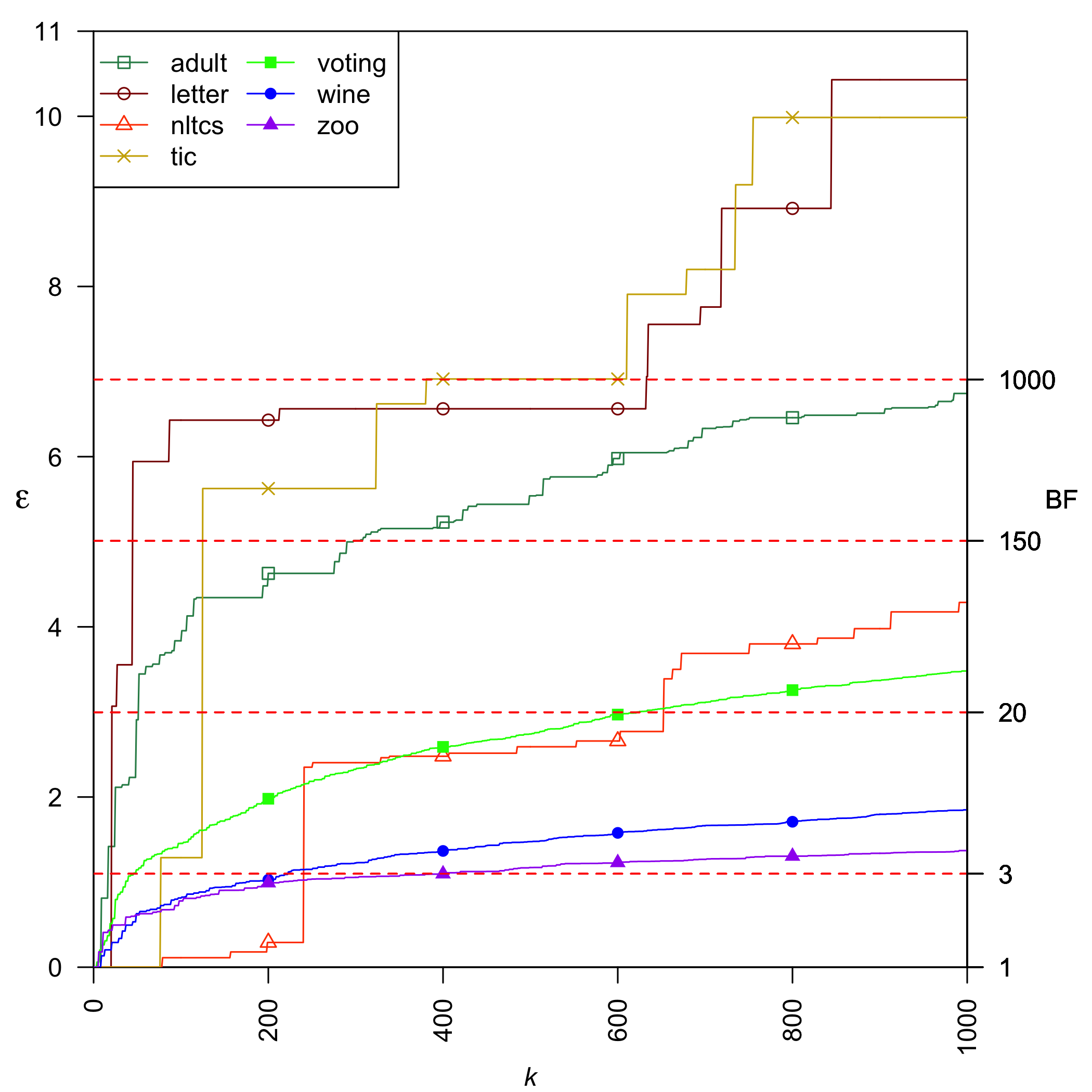
Now we show that different datasets have distinct score patterns in the top scoring networks. The scores of the 1,000-best networks for some datasets in the KBest experiment are plotted in Figure 2. A specific line for a dataset indicates the deviation $\epsilon$ from the optimal BDeu score by the $k$th-best network. For reference, the red dash lines represent different levels of BFs calculated by $\epsilon=\log{BF}$ (See Equation 3). The figure shows that it is difficult to pick a value for $k$ a priori to capture the appropriate set of top scoring networks. For a few datasets such as adult and letter, it only takes fewer than 50 networks to reach a BF of 20, whereas zoo needs more than 10,000 networks. The sample size has a significant effect on the number of networks at a given BF since the lack of data leads to many BNs with similar probabilities. It would be reasonable to choose a large value for $k$ in model averaging when data is scarce and vice versa, but only the BF approach is able to automatically find the appropriate and credible set of networks for further analysis.

6 Conclusion

Existing approaches for model averaging for Bayesian network structure learning either severely restrict the structure of the Bayesian network or have only been shown to scale to networks with fewer than 30 random variables. In this paper, we proposed a novel approach to model averaging in Bayesian network structure learning that finds all networks within a factor of optimal. Our approach has two primary advantages. First, our approach only considers credible models in that they are optimal or near-optimal in score. Second, our approach is significantly more efficient and scales to much larger Bayesian networks than existing approaches. We modified GOBNILP (Bartlett and Cussens, 2013), a state-of-the-art method for finding an optimal Bayesian network, to implement our generalized pruning rules and to find all near-optimal networks. Our experimental results demonstrate that the modified GOBNILP scales to significantly larger networks without resorting to restricting the structure of the Bayesian networks that are learned.

Appendix A Proofs of Pruning Rules

We discuss the original pruning rules and prove their generalization below. A candidate parent set $\Pi_{i}$ can be safely pruned given a non-negative constant $\epsilon\in\mathbb{R}^{+}$ if $\Pi_{i}$ cannot be the parent set of $V_{i}$ in any network in the set of credible networks. Note that proofs of the original rules can be obtained by setting $\epsilon=0$.

A.1 Proof of Lemma 3

Teyssier and Koller (2005) give a pruning rule that is applicable for all decomposable scoring functions.

Theorem 9.

(Teyssier and Koller, 2005) Given a vertex variable $V_{j}$, and candidate parent sets $\Pi_{j}$ and $\Pi_{j}^{\prime}$, if $\Pi_{j}\subset\Pi_{j}^{\prime}$ and $\sigma({\Pi_{j}})<\sigma({\Pi_{j}^{\prime}})$, $\Pi_{j}^{\prime}$ can be safely pruned.

We relax this pruning rule and prove Lemma 3 below.

Proof.

(Lemma 3) Consider networks $\mathit{G}$ and $\mathit{G}^{\prime}$ that are the same except for the parent set of $V_{j}$, where $\mathit{G}$ has the parent set $\Pi_{j}$ for $V_{j}$ and $\mathit{G}^{\prime}$ has the parent set $\Pi_{j}^{\prime}$ for $V_{j}$.

$$\sigma({\mathit{G}}) =\sigma({\Pi_{j}})+\sum_{i\neq j}\sigma({\Pi_{j}}) [\sigma({})\text{ is decomposable}]$$

$$\leq\sigma({\Pi_{j}^{\prime}})+\epsilon+\sum_{i\neq j}\sigma({\Pi_{j}}) [\text{given}]$$

$$=\sigma({\mathit{G}^{\prime}}).$$

Thus, $\mathit{G}^{\prime}$ cannot be in the set of credible networks. ∎

A.2 Proof of Theorem 4

An additional pruning rule can be derived from Theorem 9 that is applicable to the BIC/MDL scoring function.

Theorem 10.

(de Campos and Ji, 2011) Given a vertex variable $V_{i}$, and candidate parent sets $\Pi_{i}$ and $\Pi_{i}^{\prime}$, if $\Pi_{i}\subset\Pi_{i}^{\prime}$ and $\sigma({\Pi_{i}})-t({\Pi_{i}^{\prime}})<0$, $\Pi_{i}^{\prime}$ and all supersets of $\Pi_{i}^{\prime}$ can be safely pruned if $\sigma$ is the BIC/MDL scoring function.

Here, $t({\Pi_{i}^{\prime}})$ is the penalty term in the BIC scoring function. This pruning rule is relaxed as Theorem 4 and we prove it below.

Proof.

(Theorem 4)

$$\sigma({\Pi_{i}})-t({\Pi_{i}^{\prime}})+\epsilon<0 [\text{given}]$$

$$\Rightarrow-\sigma({\Pi_{i}})+t({\Pi_{i}^{\prime}})-\epsilon>0$$

$$\Rightarrow-\sigma({\Pi_{i}})+t({\Pi_{i}^{\prime}})-L(\Pi_{i}^{\prime})-\epsilon>0 [L(\Pi_{i}^{\prime})<0]$$

$$\Rightarrow\sigma({\Pi_{i}^{\prime}})>\sigma({\Pi_{i}})+\epsilon.$$

By Lemma 3, $\Pi_{i}^{\prime}$ cannot be an optimal parent set. Using the fact that penalties increase with increase in parent set size, supersets of $\Pi_{i}^{\prime}$ cannot be in the set of credible networks. The result follows. ∎

A.3 Proof of Theorem 5

Theorem 11.

(de Campos and Ji, 2011) Given a vertex variable $V_{i}$ and candidate parent set $\Pi_{i}$ such that $r_{\Pi_{i}}>\frac{N}{w}\frac{\log r_{i}}{r_{i}-1}$, if $\Pi_{i}\subsetneq\Pi_{i}^{\prime}$ , then $\Pi_{i}^{\prime}$ can be safely pruned if $\sigma$ is the BIC scoring function.

We relax the pruning rule given in Theorem 11 as Theorem 5 and prove it below.

Proof.

(Theorem 5)

$$\sigma(\Pi_{i}^{\prime})-\sigma(\Pi_{i})$$

$$\mathbin{{\mathop{=}\limits}}-\displaystyle\max_{\theta_{i}}L(\Pi_{i}^{\prime})+t(\Pi_{i}^{\prime})\cdot w+\displaystyle\max_{\theta_{i}}L(\Pi_{i})-t(\Pi_{i})\cdot w$$

$$\mathbin{{\mathop{\geq}\limits}}\displaystyle-\max_{\theta_{i}}L(\Pi_{i})+t(\Pi_{i}^{\prime})\cdot w-t(\Pi_{i})\cdot w$$

$$\mathbin{{\mathop{=}\limits}}\displaystyle-\sum_{j=1}^{r_{\Pi_{i}}}n_{ij}(-\sum^{r_{i}}_{i=1}\frac{n_{ijk}}{n_{ij}}\log\frac{n_{ijk}}{n_{ij}})+t(\Pi_{i}^{\prime})\cdot w-t(\Pi_{i})\cdot w$$

$$\mathbin{{\mathop{\geq}\limits}}\displaystyle-\sum_{j=1}^{r_{\Pi_{i}}}n_{ij}H(\theta_{ij})-t(\Pi_{i}^{\prime})\cdot w+t(\Pi_{i})\cdot w$$

$$\mathbin{{\mathop{\geq}\limits}}\displaystyle-\sum_{j=1}^{r_{\Pi_{i}}}n_{ij}\log r_{i}+r_{\Pi_{i}}\cdot(r_{e}-1)\cdot(r_{i}-1)\cdot w$$

$$\mathbin{{\mathop{\geq}\limits}}\displaystyle-\sum_{j=1}^{r_{\Pi_{i}}}n_{ij}\log r_{i}+r_{\Pi_{i}}\cdot(r_{i}-1)\cdot w$$

$$\mathbin{{\mathop{=}\limits}}-N\log r_{i}+r_{\Pi_{i}}\cdot(r_{i}-1)\cdot w$$

$$\mathbin{{\mathop{>}\limits}}\epsilon.$$

Step 0 uses the definition of $BIC$. Step 1 uses $\max_{\theta_{i}}L(\Pi_{i}^{\prime})$ is negative. Step 2 uses the fact that the maximum likelihood estimate, $\theta^{\ast}_{ijk}=\frac{n_{ijk}}{n_{ij}}$ and $n_{ij}=\sum_{i=1}^{r_{i}}n_{ijk}$. Step 3 uses the definition of entropy. Step 4 uses the definition of the penalty function $t$. Step 5 uses $r_{e}\geq 2$. Finally, the RHS in Step 6 follows because of the definition of $n_{ij}$. Step 7 uses the assumption of the theorem.

Using Lemma 3, we get the result as desired. ∎

A.4 Proof of Corollary 6

Corollary 12.

(de Campos and Ji, 2011) Given a vertex variable $V_{i}$ and candidate parent set $\Pi_{i}$, if $\Pi_{i}$ has more than $\log_{2}N$ elements, $\Pi_{i}$ can be safely pruned if $\sigma$ is the BIC scoring function.

Using Theorem 5, we generalize Corollary 12 to Corollary 6 and prove it below.

Proof.

(Corollary 6) Assuming $N>4$, take a variable $V_{i}$ and a parent set $\Pi_{i}$ with $|\Pi_{i}|=\lceil\log_{2}(N+\epsilon)\rceil$ elements. Because every variable has at least two states, we know that $r_{\Pi_{i}}\geq 2^{|\Pi_{i}|}\geq N+\epsilon>\frac{N}{w}\frac{\log r_{i}}{r_{i}-1}+\epsilon$, because $w=\log\frac{N}{2}$ gives us $\frac{\log r_{i}}{w(r_{i}-1)}<1$ , and by Theorem 5 we know that no proper superset of $\Pi_{i}$ can be an optimal parent set for $V_{i}$ as desired. ∎

A.5 Proof of Theorem 7

Lemma 13.

(de Campos et al., 2018) Given a vertex variable $V_{i}$, and candidate parent sets $\Pi_{i}$, $\Pi_{i}^{\prime}$ such that $\Pi_{i}=\Pi_{i}^{\prime}\cup\{V_{j}\}$ for some variable $V_{j}\notin\Pi_{i}^{\prime}$, we have $L(\Pi_{i})-L(\Pi_{i}^{\prime})\leq N\cdot\min\{H(V_{i}\mid\Pi_{i}^{\prime}),H(V_{j}\mid\Pi_{i}^{\prime})\}$.

Proof.

First, consider the definition of $L_{i}(\Pi_{i})$,

$$L(\Pi_{i})=\max_{\theta}\sum_{j=1}^{r_{\Pi_{i}}}\sum_{k=1}^{r_{i}}n_{ijk}\log{\theta}_{ijk},$$

where the maximum likelihood estimate of $\theta_{ijk}$ is $\frac{n_{ijk}}{n_{ij}}$. This gives us $N\cdot H(V_{i}\mid\Pi_{i})=-L(\Pi_{i})$. Thus, we get,

$$L(\Pi_{i})-L(\Pi_{i}^{\prime}) =N\cdot(H(V_{i}\mid\Pi_{i}^{\prime})-H(V_{i}\mid\Pi_{i})\mathbin{{\mathop{\leq}\limits}}N\cdot H(V_{i}\mid\Pi_{i}^{\prime}).$$

We use the fact that entropy is positive. Now, consider the definition of mutual information,

$$I(X,Y\mid Z)=H(X\mid Z)=H(X\mid Y\cup Z).$$

This gives us,

$$L(\Pi_{i})-L(\Pi_{i}^{\prime}) =N\cdot I(V_{i},V_{j}\mid\Pi_{i}^{\prime})$$

$$\mathbin{{\mathop{=}\limits}}N\cdot(H(V_{j}\mid\Pi_{i}^{\prime})-H(V_{j}\mid\Pi_{i}^{\prime}\cup\{V_{i}\}))$$

$$\Rightarrow L(\Pi_{i})-L(\Pi_{i}^{\prime}) \mathbin{{\mathop{\leq}\limits}}N\cdot\min\{H(V_{i}\mid\Pi_{i}^{\prime}),H(V_{j}\mid\Pi_{i}^{\prime})\}.$$

Step 3 combines Steps 1 and 2. The result follows as desired. ∎

Theorem 14.

(de Campos et al., 2018) Given a vertex variable $V_{i}$, and candidate parent set $\Pi_{i}$, let $V_{j}\notin\Pi_{i}$ such that $N\cdot\min\{H(V_{i}\mid\Pi_{i}),H(V_{j}\mid\Pi_{i})\}\geq(1-r_{j})\cdot t(\Pi_{i})$. Then the candidate parent set $\Pi_{i}^{\prime}=\Pi_{i}\cup\{V_{j}\}$ and all its supersets can be safely pruned if $\sigma$ is the BIC scoring function.

We relax Theorem 14 and prove its generalization below.

Proof.

(Theorem 7)

$$\sigma({\Pi_{i}^{\prime}}) \mathbin{{\mathop{=}\limits}}-L(\Pi_{i}^{\prime})+t(\Pi_{i}^{\prime})$$

$$\mathbin{{\mathop{\geq}\limits}}-L(\Pi_{i})-N\cdot\min\{H(V_{i}\mid\Pi_{i});H(V_{j}\mid\Pi_{i})\}+t(\Pi_{i}^{\prime})$$

$$\mathbin{{\mathop{\geq}\limits}}-L(\Pi_{i})+(1-r_{j})\cdot t(\Pi_{i})+\epsilon+t(\Pi_{i}^{\prime})$$

$$\mathbin{{\mathop{=}\limits}}-L(\Pi_{i})+t(\Pi_{i})-r_{j}\cdot t(\Pi_{i})+\epsilon+t(\Pi_{i}^{\prime})$$

$$\mathbin{{\mathop{=}\limits}}-L(\Pi_{i})+t(\Pi_{i})-r_{j}\cdot r_{\Pi_{i}}\cdot(r_{i}-1)+\epsilon+t(\Pi_{i}^{\prime})$$

$$\mathbin{{\mathop{=}\limits}}-L(\Pi_{i})+t(\Pi_{i})-t(\Pi_{i}^{\prime})+\epsilon+t(\Pi_{i}^{\prime})$$

$$\mathbin{{\mathop{=}\limits}}\sigma({\Pi_{i}})+\epsilon.$$

Step 1 uses Lemma 13. Step 2 uses the assumptions of the question. Step 4 uses the definition of $t$. Step 5 uses $\Pi_{i}^{\prime}=\Pi_{i}\cup\{V_{j}\}$. Using Lemma 3, the result follows as desired. ∎

A.6 Proof of Theorem 8

Lemma 15.

Let $n_{ij}$ be a positive integer and $\alpha^{\prime}$ be a positive real number. Then

$$\log\frac{\Gamma(n_{ij}+\alpha^{\prime})}{\Gamma(\alpha^{\prime})}=\sum_{i=0}^{n_{ij-1}}\log(i+\alpha^{\prime})$$

Proof.

We start with the property that $\Gamma(x+1)=x\Gamma(x)$ for any positive real number $x$. As $\alpha^{\prime}>0$, this gives us,

$$\frac{\Gamma(1+\alpha^{\prime})}{\Gamma(\alpha^{\prime})} \mathbin{{\mathop{=}\limits}}\alpha^{\prime}$$

$$\frac{\Gamma(2+\alpha^{\prime})}{\Gamma(1+\alpha^{\prime})} \mathbin{{\mathop{=}\limits}}(1+\alpha^{\prime})$$

$$\Rightarrow\frac{\Gamma(1+\alpha^{\prime})\cdot\Gamma(2+\alpha^{\prime})}{\Gamma(1+\alpha^{\prime})\Gamma(\alpha^{\prime})} \mathbin{{\mathop{=}\limits}}\alpha^{\prime}(1+\alpha^{\prime})$$

$$\Rightarrow\frac{\Gamma(1+\alpha^{\prime})\cdots\Gamma(n_{ij}+\alpha^{\prime})}{\Gamma(n_{ij}-1+\alpha^{\prime})\cdots\Gamma(\alpha^{\prime})} \mathbin{{\mathop{=}\limits}}\alpha^{\prime}\cdots(n_{ij}-1+\alpha^{\prime})$$

$$\Rightarrow\frac{\Gamma(n_{ij}+\alpha^{\prime})}{\Gamma(\alpha^{\prime})} \mathbin{{\mathop{=}\limits}}\alpha^{\prime}\cdots(n_{ij}-1+\alpha^{\prime})$$

$$\Rightarrow\log\frac{\Gamma(n_{ij}+\alpha^{\prime})}{\Gamma(\alpha^{\prime})} \mathbin{{\mathop{=}\limits}}\sum_{i=0}^{n_{ij-1}}\log(i+\alpha^{\prime}).$$

Step 1 uses $1+\alpha^{\prime}$. Step 2 follows by multiplication of the equations in Step 1 and Step 0. Step 3 follows by repeated application of the identity. Step 4 cancels identical terms in the LHS. The result follows as desired. ∎

Lemma 16.

6B Let $\{n_{ijk}\}_{k=1,...r_{i}}$ be non-negative integers with a positive sum, $n_{ij}=\sum_{k=1}^{r_{i}}n_{ijk}$ and $\alpha^{\prime\prime}$ be a positive real number. Then

$$\sum_{k=1}^{r_{i}}\log\frac{\Gamma(n_{ijk}+\alpha^{\prime\prime})}{\Gamma(\alpha^{\prime\prime})}\leq\log\frac{\Gamma(n_{ij}+\alpha^{\prime\prime})}{\Gamma(\alpha^{\prime\prime})}$$

Proof.

Consider allocation of $\{n_{ijk}\}_{k=1,...,{r_{i}}}$ items over the $r_{i}$ bins. There are two cases.

• Let there be some index $k^{\ast}$ such that $n_{ijk^{\ast}}=n_{ij}$. This means that $n_{ijk}=0$ for all $k\neq k^{\ast}$. It follows that $\sum_{k=1}^{r_{i}}\log\frac{\Gamma(n_{ijk}+\alpha^{\prime\prime})}{\Gamma(\alpha^{\prime\prime})}=\log\frac{\Gamma(n_{ij}+\alpha^{\prime\prime})}{\Gamma(\alpha^{\prime\prime})}$.

• Let there be two indices $k_{1}$ and $k_{2}$ such that $n_{ijk_{1}}>0$ and $n_{ijk_{2}}>0$. Without loss of generality, we can assume that $n_{ijk_{1}}\geq n_{ijk_{2}}$. We move one item from bin $k_{1}$ to bin $k_{2}$. The sum $n_{ij}$ remains constant. By Lemma 15, an increase in the RHS by $\log(n_{ijk_{1}}+\alpha^{\prime\prime})-\log(n_{ijk_{2}}-1+\alpha^{\prime\prime})$, results in a corresponding increase in the LHS. Note that the assumption $n_{ijk_{1}}\geq n_{ijk_{2}}$ means that this increase is positive. By increasing counts at the expense of small counts in this way a sequence of distributions of the fixed sum $n_{ij}$ over the $r_{i}$ bins can be constructed for which the LHS of Lemma 16 is increasing. The sequence terminates when $n_{ijk^{\ast}}=n_{ij}$ for some $k^{\ast}$. The result follows.

∎

Theorem 17.

Correia et al. (2020)

$$\sum_{j=1}^{r_{\Pi_{i}}}\Bigg(\frac{\Gamma(\alpha^{\prime})}{\Gamma(n_{ij}+\alpha^{\prime})}+\sum_{k=1}^{r_{i}}\log\frac{\Gamma(n_{ijk}+\frac{\alpha^{\prime}}{r_{i}})}{\Gamma(\frac{\alpha^{\prime}}{r_{i}})}\Bigg)\leq\sum_{i=0,j:n_{ij}>0}^{n_{ij}}\log\Big(\frac{i+a^{\prime}/r_{i}}{i+\alpha}\Big).$$

Proof.

$$\sum_{j=1}^{r_{\Pi_{i}}}\Bigg(\log\frac{\Gamma(\alpha^{\prime})}{\Gamma(n_{ij}+\alpha^{\prime})}+\sum_{k=1}^{r_{i}}\log\frac{\Gamma(n_{ijk}+\frac{\alpha^{\prime}}{r_{i}})}{\Gamma(\frac{\alpha^{\prime}}{r_{i}})}\Bigg)$$

$$\mathbin{{\mathop{\leq}\limits}}\sum_{j=1}^{r_{\Pi_{i}}}\Bigg(\log\frac{\Gamma(\alpha^{\prime})}{\Gamma(n_{ij}+\alpha^{\prime})}+\log\frac{\Gamma(n_{ij}+\frac{\alpha^{\prime}}{r_{i}})}{\Gamma(\frac{\alpha^{\prime}}{r_{i}})}\Bigg)$$

$$\mathbin{{\mathop{\leq}\limits}}\sum_{j=1}^{r_{\Pi_{i}}}\Bigg(\log\frac{\Gamma(\alpha^{\prime})}{\Gamma(n_{ij}+\alpha^{\prime})}\frac{\Gamma(n_{ij}+\frac{\alpha^{\prime}}{r_{i}})}{\Gamma(\frac{\alpha^{\prime}}{r_{i}})}\Bigg)$$

$$\mathbin{{\mathop{\leq}\limits}}\sum_{i=0,j:n_{ij}>0}^{n_{ij}-1}\Big(\log\frac{i+a^{\prime}/r_{i}}{i+\alpha^{\prime}}\Big)$$

$$\mathbin{{\mathop{\leq}\limits}}\sum_{i=0,j:n_{ij}>0}^{n_{ij}}\log\Big(\frac{i+a^{\prime}/r_{i}}{i+\alpha^{\prime}}\Big).$$

Step 1 uses Lemma 16. Step 2 assumes $n_{ij}>0$, and uses properties of the logarithm function. Step 3 uses Lemma 15. The result follows as desired. ∎

Corollary 18.

(Correia et al., 2020) Given that $r_{i}^{+}:=|\{j:n_{ij}>0\}|$, then

$$\sum_{j=1}^{r_{\Pi_{i}}}\log\frac{\Gamma(\alpha^{\prime})}{\Gamma(n_{ij}+\alpha^{\prime})}+\sum_{k=1}^{r_{i}}\log\frac{\Gamma(n_{ijk}+\frac{\alpha^{\prime}}{r_{i}})}{\Gamma(\frac{\alpha^{\prime}}{r_{i}})}\leq-r_{i}^{+}\log r_{i}.$$

Proof.

If $n_{ij}>0$, then

$$\sum_{i=0}^{n_{ij}}\log\Big(\frac{i+a^{\prime}/r_{i}}{i+\alpha^{\prime}}\Big) =-\log r_{i}\sum_{i=1}^{n_{ij}}\log\Big(\frac{i+a^{\prime}/r_{i}}{i+\alpha^{\prime}}\Big)\leq-\log r_{i}.$$

Note that as $r_{i}\geq 2$, and $\alpha^{\prime}>0$, it is clear that $i+\alpha^{\prime}/r_{i}<i+\alpha^{\prime}$. This means that each term in $\sum_{i=1}^{n_{ij}}\log\Big(\frac{i+a^{\prime}/r_{i}}{i+\alpha^{\prime}}\Big)$ is negative. This gives us the second inequality. The result then follows from Theorem 17 as desired. ∎

Corollary 19.

(Correia et al., 2020) Given a vertex variable $V_{i}$ and candidate parent sets $\Pi_{i}$ and $\Pi_{i}^{\prime}$ such that $\Pi_{i}\subset\Pi_{i}^{\prime}$ and $\Pi_{i}\neq\Pi_{i}^{\prime}$, let $r_{i}^{+}(\Pi_{i}^{\prime})$ be the number of positive counts in the contingency table for $\Pi_{i}^{\prime}$. If $\sigma({\Pi_{i}})<r_{i}^{+}(\Pi_{i}^{\prime})\log r_{i}$ then $\Pi_{i}^{\prime}$ and the supersets of $\Pi_{i}^{\prime}$ can be safely pruned.

We generalize Corollary 19 to Theorem 8 and prove it below.

Proof.

(Theorem 8) Let $G^{\prime}$ be a Bayesian network where $\Pi_{i}^{\prime}$ or one of its supersets is a parent set for $V_{i}$. Let $G$ be another Bayesian network where $\Pi_{i}$ is the parent set for $V_{i}$.

Consider the LHS of Corollary 18. It is the local BDeu score for a parent set $\Pi_{i}^{\prime}$ which has $r_{\Pi_{i}}$ counts $n_{ij}$ in its contingency table and counts $n_{ijk}$ in the contingency table for $\Pi_{i}^{\prime}\cup\{V_{i}\}$, where $\alpha^{\prime}=\alpha/r_{\Pi_{i}}$ for some ESS $\alpha$. If $r_{i}^{+}$($\Pi_{i}^{\prime})\log r_{i}>\sigma({\Pi_{i}})+\epsilon$ then $\sigma({\Pi_{i}})+\epsilon$ is lower than the local BDeu score for $\Pi_{i}^{\prime}$ due to Corollary 18. Take a candidate parent set $\Pi_{i}^{\prime\prime}$. If $\Pi_{i}^{\prime}\subset\Pi_{i}^{\prime\prime}$ then $r_{i}^{+}(\Pi_{i}^{\prime\prime})\leq r_{i}^{+}(\Pi_{i}^{\prime})$ and so $r_{i}^{+}(\Pi_{i}^{\prime\prime})\log r_{i}\leq r_{i}^{+}(\Pi_{i}^{\prime})\log r_{i}$, as $r_{i}\geq 2$. From this it follows that the local score for $\Pi_{i}^{\prime\prime}$ must also be more than $\sigma({\Pi_{i}})+\epsilon$. Using Lemma 3, the result follows as desired. ∎

References

- Bartlett and Cussens (2013) Mark Bartlett and James Cussens. Advances in Bayesian network learning using integer programming. In Proceedings of the 29th Conference on Uncertainty in Artificial Intelligence, pages 182–191, 2013.
- Buntine (1991) Wray L. Buntine. Theory refinement of Bayesian networks. In Proceedings of the Seventh Conference on Uncertainty in Artificial Intelligence, pages 52–60, 1991.
- Chen et al. (2015) Eunice Yuh-Jie Chen, Arthur Choi, and Adnan Darwiche. Learning Bayesian networks with non-decomposable scores. In Proceedings of the 4th IJCAI Workshop on Graph Structures for Knowledge Representation and Reasoning (GKR 2015), pages 50–71, 2015. Available as: LNAI 9501.
- Chen et al. (2016) Eunice Yuh-Jie Chen, Arthur Choi, and Adnan Darwiche. Enumerating equivalence classes of Bayesian networks using EC graphs. In Proceedings of the 19th International Conference on Artificial Intelligence and Statistics (AISTATS), pages 591–599, 2016.
- Chen et al. (2018) Eunice Yuh-Jie Chen, Adnan Darwiche, and Arthur Choi. On pruning with the MDL score. International Journal of Approximate Reasoning, 92:363–375, 2018.
- Chen and Tian (2014) Yetian Chen and Jin Tian. Finding the -best equivalence classes of Bayesian network structures for model averaging. In Proceedings of the 28th Conference on Artificial Intelligence, pages 2431–2438, 2014.
- Claeskens and Hjort (2008) Gerda Claeskens and Nils Lid Hjort. Model Selection and Model Averaging. Cambridge University Press, 2008.
- Correia et al. (2020) Alvaro HC Correia, James Cussens, and Cassio P de Campos. On pruning for score-based bayesian network structure learning. In The 23rd International Conference on Artificial Intelligence and Statistics, 2020.
- Darwiche (2009) Adnan Darwiche. Modeling and Reasoning with Bayesian Networks. Cambridge University Press, 2009.
- Dash and Cooper (2004) Denver Dash and Gregory F. Cooper. Model averaging for prediction with discrete Bayesian networks. Journal of Machine Learning Research, 5:1177–1203, 2004.
- de Campos and Ji (2011) Cassio P. de Campos and Qiang Ji. Efficient structure learning of Bayesian networks using constraints. J. Mach. Learn. Res., 12:663–689, 2011.
- de Campos et al. (2018) Cassio P. de Campos, Mauro Scanagatta, Giorgio Corani, and Marco Zaffalon. Entropy-based pruning for learning Bayesian networks using BIC. Artificial Intelligence, 260:42–50, 2018.
- Dheeru and Karra Taniskidou (2017) Dua Dheeru and Efi Karra Taniskidou. UCI machine learning repository, 2017. URL http://archive.ics.uci.edu/ml.
- Gleixner et al. (2018) Ambros Gleixner, Michael Bastubbe, Leon Eifler, Tristan Gally, Gerald Gamrath, Robert Lion Gottwald, Gregor Hendel, Christopher Hojny, Thorsten Koch, Marco E. Lübbecke, Stephen J. Maher, Matthias Miltenberger, Benjamin Müller, Marc E. Pfetsch, Christian Puchert, Daniel Rehfeldt, Franziska Schlösser, Christoph Schubert, Felipe Serrano, Yuji Shinano, Jan Merlin Viernickel, Matthias Walter, Fabian Wegscheider, Jonas T. Witt, and Jakob Witzig. The SCIP Optimization Suite 6.0. Technical report, Optimization Online, July 2018. URL http://www.optimization-online.org/DB_HTML/2018/07/6692.html.
- He et al. (2016) Ru He, Jin Tian, and Huaiqing Wu. Bayesian learning in Bayesian networks of moderate size by efficient sampling. Journal of Machine Learning Research, 17:1–54, 2016.
- Heckerman et al. (1995) David Heckerman, Dan Geiger, and David M. Chickering. Learning Bayesian networks: The combination of knowledge and statistical data. Machine Learning, 20:197–243, 1995.
- Hoeting et al. (1999) Jennifer A. Hoeting, David Madigan, Adrian E. Raftery, and Chris T. Volinsky. Bayesian model averaging: A tutorial. Statistical Science, 14(4):382–401, 1999.
- Jeffreys (1967) Sir Harold Jeffreys. Theory of Probability: 3d Ed. Clarendon Press, 1967.
- Kass and Raftery (1995) Robert E. Kass and Adrian E. Raftery. Bayes factors. Journal of the American Statistical Association, 90(430):773–795, 1995.
- Koivisto and Sood (2004) Mikko Koivisto and Kismat Sood. Exact Bayesian structure discovery in Bayesian networks. J. Mach. Learn. Res., 5:549–573, 2004.
- Koller and Friedman (2009) Daphne Koller and Nir Friedman. Probabilistic Graphical Models: Principles and Techniques. The MIT Press, 2009.
- Lam and Bacchus (1994) Wai Lam and Fahiem Bacchus. Using new data to refine a Bayesian network. In Proceedings of the Tenth Conference on Uncertainty in Artificial Intelligence, pages 383–390, 1994.
- Madigan and Raftery (1994) David Madigan and Adrian E. Raftery. Model selection and accounting for uncertainty in graphical models using Occam’s window. Journal of the Amercian Statistical Association, 89:1535–1546, 1994.
- Meilă and Jaakkola (2000) Marina Meilă and Tommi Jaakkola. Tractable Bayesian learning of tree belief networks. In Proceedings of the 16th Conference on Uncertainty in Artificial Intelligence, pages 380–388, 2000.
- Ripley (1996) Brian D. Ripley. Pattern recognition and neural networks. Cambridge University Press, 1996.
- Schwarz (1978) Gideon Schwarz. Estimating the dimension of a model. The Annals of Statistics, 6:461–464, 1978.
- Silander and Myllymäki (2006) Tomi Silander and Petri Myllymäki. A simple approach for finding the globally optimal Bayesian network structure. In Proceedings of the 22nd Conference on Uncertainty in Artificial Intelligence, pages 445–452, 2006.
- Teyssier and Koller (2005) Marc Teyssier and Daphne Koller. Ordering-based search: A simple and effective algorithm for learning Bayesian networks. In Proceedings of the 21st Conference on Uncertainty in Artificial Intelligence, pages 548–549, 2005.
- Tian et al. (2010) Jin Tian, Ru He, and Lavanya Ram. Bayesian model averaging using the k-best Bayesian network structures. In Proceedings of the 26th Conference on Uncertainty in Artificial Intelligence, pages 589–597, 2010.
- van Beek and Hoffmann (2015) Peter van Beek and Hella-Franziska Hoffmann. Machine learning of Bayesian networks using constraint programming. In Proceedings of the 21st International Conference on Principles and Practice of Constraint Programming, pages 428–444, 2015.
- Verma and Pearl (1990) Thomas Verma and Judea Pearl. Equivalence and synthesis of causal models. In Proceedings of the Sixth Conference on Uncertainty in Artificial Intelligence, pages 220–227, 1990.