Managing connected and automated vehicles with flexible routing at “lane-allocation-free” intersections

Abstract

Trajectory planning and coordination for connected and automated vehicles (CAVs) have been studied at isolated “signal-free” intersections and in “signal-free” corridors under the fully CAV environment in the literature. Most of the existing studies are based on the definition of approaching and exit lanes. The route a vehicle takes to pass through an intersection is determined from its movement. That is, only the origin and destination arms are included. This study proposes a mixed-integer linear programming (MILP) model to optimize vehicle trajectories at an isolated “signal-free” intersection without lane allocation, which is denoted as “lane-allocation-free” (LAF) control. Each lane can be used as both approaching and exit lanes for all vehicle movements including left-turn, through, and right-turn. A vehicle can take a flexible route by way of multiple arms to pass through the intersection. In this way, the spatial-temporal resources are expected to be fully utilized. The interactions between vehicle trajectories are modeled explicitly at the microscopic level. Vehicle routes and trajectories (i.e., car-following and lane-changing behaviors) at the intersection are optimized in one unified framework for system optimality in terms of total vehicle delay. Considering varying traffic conditions, the planning horizon is adaptively adjusted in the implementation procedure of the proposed model to make a balance between solution feasibility and computational burden. Numerical studies validate the advantages of the proposed LAF control in terms of both vehicle delay and throughput with different demand structures and temporal safety gaps.

1 Introduction

With increasing traffic demand, vehicles suffer from severe traffic congestion, which causes environmental problems and economic losses (Koonce et al., 2008). Intersections are usually regarded as the bottlenecks for traffic flows in an urban road network. Traffic management at intersections is crucial to ensuring traffic efficiency, safety, energy economics, and pollution reduction. Conventionally, priority rules (e.g., stop signs, roundabouts, right-before-left, etc.) and traffic signals are used to assign rights of way (ROW) to conflicting traffic flows at an intersection. Fixed-time control, vehicle-actuated control, and adaptive control are widely used in practice in terms of traffic signal control (Papageorgiou et al., 2003). Numerous studies have been dedicated to these research areas (Allsop, 1976; Webster, 1958; Little et al., 1981; Heydecker, 1992; Han et al., 2014; Han and Gayah, 2015; Liu and Smith, 2015; Memoli et al., 2017; Mohebifard and Hajbabaie, 2019; Mohajerpoor et al., 2019).

With the popularity of connected and automated vehicles (CAVs), the advances in CAV technologies are likely to produce a revolution in traffic management (Li et al., 2014a; Pei et al., 2019). The communications between vehicles (V2V) and between vehicles and infrastructures (V2I) can convey traffic information (e.g., signal timings, route guidance, and speed advisory) from intersections to vehicles. At the same time, detailed vehicle trajectory data (e.g., locations and speeds) can be collected from vehicles for traffic management at intersections. As CAVs are controllable, vehicle trajectory control becomes available besides conventional signal control. It is expected that traffic control would be implemented in both temporal and spatial dimensions.

A thorough review of the research on urban traffic signal control with CAVs was provided in Guo et al. (2019a). Generally, related studies fall into three categories. In the first category, real-time vehicle trajectory information (e.g., speeds and locations) is utilized for signal optimization with or without infrastructure-based detector data (e.g., traffic volumes from loop detectors) by catching real time traffic demand (Gradinescu et al. (2007)) or temporal fluctuation (Feng et al. (2018a)). Signal timings such as cycle lengths and green splits are optimized at isolated intersections (Gradinescu et al., 2007; Guler et al., 2014; Feng et al., 2015; Liang et al., 2018; Yang et al., 2017) and multiple intersections (He et al., 2012; Yang et al., 2017). The studies in the second category focus on vehicle trajectory planning on the basis of traffic information from intersections. One typical application is eco-driving, which optimizes vehicle trajectories with the objectives of minimizing fuel/energy consumption and emission. Typically, optimal control models or feedback control models are formulated with vehicle speeds or acceleration rates as the control variables (Kamal et al., 2013; Wang et al., 2014a; Wang et al., 2014b; Ubiergo and Jin, 2016; Wan et al., 2016). Platooning can also be considered (Liu et al. (2019); Feng et al. (2019)). Approximation has then been proposed to solve the models more efficiently by either discretizing time or segmenting trajectories (Wan et al., 2016; Kamalanathsharma and Rakha, 2013). In the third category, signal optimization and vehicle trajectory planning are integrated into one unified framework. However, limited studies have been reported. Li et al. (2014b) enumerated feasible signal plans and segmented vehicle trajectories for the joint optimization. Feng et al. (2018b) proposed a dynamic programming model for signal optimization combined with an optimal control model for trajectory planning as a two-stage model. Yu et al. (2018) proposed a mixed-integer linear programming (MILP) model to simultaneously optimize signal timings and vehicle trajectories. Guo et al. (2019b) proposed a DP-SH (dynamic programming with shooting heuristic) algorithm for efficiency and jointly optimization of vehicle trajectories and signal timings.

Assuming the fully CAV environment, the concept of “signal-free” intersections has been proposed (Dresner and Stone, 2004; Dresner and Stone, 2008). Vehicles cooperate with each other and pass through intersections without physical traffic signals. One prevailing category of such studies are based on the philosophy of reservation. Approaching vehicles send requests to the intersection controller to reserve space and time slots within the intersection area. Reservation requests are managed to determine the service sequence of the approaching vehicles, usually according to rule-based policies such as “first-come, first-served” (FCFS) strategy (Au and Stone, 2010; Dresner and Stone, 2004; Dresner and Stone, 2008; Li et al., 2013), priority strategy (Alonso et al., 2011), auction strategy (Carlino et al., 2013), and platooning strategy (Tachet et al., 2016). However, both theoretical analysis (Yu et al., 2019b) and numerical case studies (Levin et al., 2016) showed that the advantages of reservation-based control might not outperform conventional signal control (e.g., vehicle-actuated control) in certain cases. Because the optimality cannot be guaranteed due to the rule-based nature of reservation-based control. As a result, optimization-based models have been proposed. In Qian et al. (2019), the scheduling algorithm can assign a feasible time to each arriving AV with low complexity. Trajectory level optimization models are more likely to take advantage of fully CAV environment. Typically, constrained nonlinear optimization models are formulated (Joyoung Lee, 2012; Zohdy and Rakha, 2016). In Joyoung Lee (2012), vehicle acceleration/deceleration rates were optimized to minimize trajectory overlap with the focus on safety. In Zohdy and Rakha (2016), vehicle arrival times at an intersection were optimized to minimize vehicle delay with the focus on efficiency. In addition, 3D CAV trajectories were mathematically formulated in the combined temporal-spatial domains (Li et al., 2019). Priority-based and Discrete Forward-Rolling Optimal Control (DFROC) algorithms were developed for CAV management at isolated intersections. The optimization of lane allocation is also considered in existing research, and proposed CAV control Distributed control methods have also been investigated to alleviate computational burden. Xu et al. (2018) projected approaching vehicles from different traffic movements into a virtual lane and then introduced a conflict-free geometry topology with the consideration of the conflict relationship of involved vehicles. Mirheli et al. (2019) proposed a vehicle-level mixed-integer non-linear programming model for cooperative trajectory planning in a distributed way. Vehicle-level solutions were pushed towards the global optimality.

Notwithstanding the abundant studies, it is noted that most of the studies do not take into consideration the interactions of vehicle trajectories at the microscopic level, which, however, is crucial to vehicle trajectory planning. Car-following behaviors are usually explicitly modeled while lane-changing behaviors are not. Recently, Yu et al. (2019a) successfully addressed this issue. Both car-following and lane-changing behaviors of vehicles in a “signal-free” corridor were cooperatively optimized in one unified framework. Approaching lanes were not specified with lane allocation, which is called “approaching-lane-allocation-free” (ALAF) in this paper. Each approaching lane could be used by all vehicle movements (i.e., left-turn, through, and right-turn). This study takes a further step and eliminates the definition of approaching and exit lanes. Acctually, it has been proved that the break of the traditional division between approchang lanes and exiting lanes brings higher control efficiency (Mitrovic et al., 2020; Sun et al., 2017). However, the lane allocations at intersections are fixed in these studies, and the innovation which not divide traffic flows in directions is limited in link scope. The dynamic lane allocation assignment is not considered. In this study, the lane allocations of all lanes are elimited. Each lane can be used by both approaching and leaving vehicles in all directions. Further, the route a vehicle takes to pass through the intersection is fixed in Yu et al. (2019a), which only consists of the origin and the destination arms. In this study, a vehicle can take a flexible route by way of multiple arms. In this way, the spatial-temporal resources at intersections are expected to be fully utilized, especially with imbalanced traffic. To this end, this study proposes an MILP model to optimize vehicle routes and trajectories (i.e., car-following behaviors and lane changing behaviors) at an isolated “signal-free” and “lane-allocation-free” intersection, which is denoted as “lane-allocation-free” (LAF) control. To balance solution feasibility and computational burden, the planning horizon is adaptively adjusted in the implementation procedure with varying traffic conditions.

The remainder of this paper is organized as follows. Section 2 describes the problem and presents the notations. Section 3 formulates the MILP model to optimize vehicle routes and trajectories at a “signal-free” and “lane-allocation-free” intersection. Section 4 presents the implementation procedure of the proposed model with varying traffic conditions, which adaptively adjusts the planning horizon to improve computational efficiency. Numerical studies are conducted in Section 5.Finally, conclusions and recommendations are provided in Section 6.

2 Problem description and notations

2.1 Problem description

Fig. 1 shows a “signal-free” and “lane-allocation-free” intersection with four arms as an example. In this study, one arm consists of an undirected link and all directed connectors departing from the link. For example, arm 1 has four connectors for left-turn traffic, four for through traffic, and four for right-turn traffic. Fig. 1 highlights the link part and the connector part of arm 1. In contrast with conventional intersections, no approaching lanes or exit lanes are defined, and no lane allocation is specified. That is, each lane can be used by both approaching and leaving vehicles in all directions in the control zone at the intersection.

Figure 1: A “signal-free” and “lane-allocation-free” intersection with four arms.

Conventionally, the route of a vehicle is fixed at an intersection. For example, vehicle $\omega$ in arm 1 tries to turn left in Fig. 1. It turns left directly similar with the trajectory of vehicle $\omega_{1}$ under conventional traffic management. That is, the route of vehicle $\omega$ only consists of arm 1 and arm 2. If vehicle $\omega$ conflicts with other vehicles, it may wait at the stop bar location, blocking the traffic behind. Suppose there is heavy through traffic, light left-turn traffic in arm 1 and light traffic in arm 4. Left-turn vehicle $\omega$ is waiting in the rightmost lane in arm 1, looking for the gaps between the through vehicles in the remaining three lanes. As a result, only three lanes in arm 1 can be fully utilized at the same time. To improve the efficiency of the intersection system, flexible routing is considered in this study. Routing means that vehicle $\omega$ can travel to other arms before entering the destination arm 2, e.g., following the trajectory of vehicle $\omega_{3}$. In this way, vehicle $\omega$ can wait in arm 4 instead of arm 1 and the four lanes in arm 1 can be fully utilized by the heavy through traffic. The trajectory of vehicle $\omega_{2}$ is another possible route. In this way, it is expected the spatial-temporal resources can be better utilized at the intersection.

Given the geometric layout of the intersection and the vehicles in the control zone ($L_{a}$), the objective of this study is to cooperatively optimize the routes and the trajectories of the vehicles for minimizing total delay. The route plan of vehicle $\omega$ is the selection of arms to be visited between the origin arm $a_{0}^{\omega}$, in which vehicle $\omega$ is traveling, and the destination arm $a_{out}^{\omega}$ as well as the arm sequence. The trajectory of vehicle $\omega$ is determined by the lane choice ($\delta_{k}^{\omega}(t)$) and the longitudinal location ($x_{a}^{\omega}(t)$) in each visited arm at each time step $t$. Note that $a_{0}^{\omega}$ is updated when vehicle $\omega$ enters a new arm. For example, $a_{0}^{\omega}$ is arm 1 in Fig. 1 and vehicle $\omega$ follows the trajectory of vehicle $\omega_{3}$. $a_{0}^{\omega}$ becomes arm 4 when vehicle $\omega$ travels in arm 4. $\mathbf{A}^{\omega}$ is then introduced to store the arms that vehicle $\omega$ has not visited. In Fig. 1, $\mathbf{A}^{\omega}=\left\{\mathrm{arm}\ 2,\mathrm{arm}\ 3,\mathrm{arm}\ 4\right\}$ when vehicle $\omega$ is in arm 1 and $\mathbf{A}^{\omega}=\left\{\mathrm{arm}\ 2,\mathrm{arm}\ 3\right\}$ when vehicle $\omega$ travels into arm 4.

To simplify the formulations, the following assumptions are made:

• All vehicles are CAVs and can be controlled by a centralized controller.

• The destination arm of a vehicle does not change after the vehicle enters the control zone.

• Vehicles follow the connectors and do not change lanes when traveling within the intersection area.

• Vehicles travel at constant speeds in connectors. The speed is determined by the radius of a connector.

• Vehicles can change lanes instantly in the link part of each arm.

• Vehicle motion is captured by the first order model, the same assumption as in Newell’s car-following model (Newell, 2002).

2.2 Notations

Main notations applied hereafter are summarized in Table 1. They will be explained in detail in the formulations.

Table 1: Notations

General notations
$\mathrm{M}$:	A sufficiently large number
$t$:	Time step
$\boldsymbol{\Omega}$:	Set of vehicles in the control zone of the intersection; each vehicle is denoted as $\omega$
$\mathbf{A}$:	Set of arms of the intersection; each arm is denoted as $a$
$a_{0}^{\omega}$:	Origin arm in which vehicle $\omega$ is traveling when the optimization is conducted
$a_{out}^{\omega}$:	Destination arm in which vehicle $\omega$ leaves the control zone of the intersection
$\mathbf{A}^{\omega}$:	Set of arms that vehicle $\omega$ has not visited; if vehicle $\omega$ is in arm $a_{out}^{\omega}$, then $\mathbf{A}^{\omega}=\emptyset$
$\mathbf{A}_{0}^{\omega}$:	Set of arms that vehicle $\omega$ is visiting or has not visited; $\mathbf{A}_{0}^{\omega}=\mathbf{A}^{\omega}\cup\left\{a_{0}^{\omega}\right\}$
$\mathbf{K}_{a}$:	Set of lanes in arm $a$; each lane is denoted as $k$
$\mathbf{K}_{a}^{left}$:	The leftmost lane of arm $a$
$\mathbf{K}_{a}^{right}$:	The rightmost lane of arm $a$
$k^{left}$:	The left adjacent lane of lane $k$ with facing the stop line
$k^{right}$:	The right adjacent lane of lane $k$ with facing the stop line
$\mathbf{K}_{a_{1}}^{a_{2}}$:	Set of lanes in arm $a_{1}$ that are connected to the lanes in arm $a_{2}$
$\mathbf{K}_{out}^{\omega}$:	Set of lanes in the destination arm in which vehicle $\omega$ leaves the control zone
$k_{+}^{a}$:	Succeeding lane of lane $k$ in arm $a$; that is, lane $k_{+}^{a}$ is connected from lane $k$ by a connector
$\left\langle k_{1},k_{2}\right\rangle$:	Connector from lane $k_{1}$ to lane $k_{2}$
$\mathbf{P}_{k_{1},k_{2}}^{k_{3},k_{4}}$:	Set of conflict points between connector $\left\langle k_{1},k_{2}\right\rangle$ and connector $\left\langle k_{3},k_{4}\right\rangle$; each conflict point is denoted as $p$
Parameters
$\Delta t$:	Length of time step, s
$t_{0}$:	Current time when vehicle routes and trajectories are optimized, which indicates the start of the planning horizon (i.e., $t=0$), s
$T$:	Planning horizon; the horizon duration is $T\cdot\Delta t$
$T_{0}$:	Initial value of $T$ in the implementation procedure for adaptively adjusting $T$
$\Delta T$:	Step length for adjusting $T$ in the implementation procedure
$T^{turn}$:	Time steps of turnning around; the turnning around time is $T^{turn}\cdot\Delta t$
$L_{a}$:	Length of the link part of arm $a$ in the control zone, m
$V_{a}$:	Speed limit on the link part of arm $a$, m/s
$l_{k_{1}}^{k_{2}}$:	Length of connector $\left\langle k_{1},k_{2}\right\rangle$ that connects lane $k_{1}$and lane $k_{2}$, m
$l_{k_{1},k_{2}}^{p}$:	Distance between the start of connector $\left\langle k_{1},k_{2}\right\rangle$ and conflict point $p$, m
$v_{k_{1}}^{k_{2}}$:	Travel speed in connector $\left\langle k_{1},k_{2}\right\rangle$, m/s
$\tau$:	Temporal safety gap, s
$d:$	Spatial safety gap, m
$\tilde{x}^{\omega}$:	Distance between vehicle $\omega$ and the stop bar location in the current arm at the current time step, m
$\tilde{\delta}_{k}^{\omega}$:	1, if vehicle $\omega$ is in lane $k$ in the current arm at the current time step; 0, otherwise
$\tilde{dir}_{a}^{\omega}$:	1, if vehicle $\omega$ driving toward the stop line; 0, otherwise
$\tilde{\gamma}_{a_{1},a_{2}}^{\omega}$:	1, if vehicle $\omega$ plans to travel from arm $a_{1}$ to arm $a_{2}$ according the previous optimization; 0, otherwise
$\underline{t}_{0}^{\omega}$:	Recorded the time point when vehicle $\omega$ entered the link part of the current arm, which is a relative value to the current time, s
$\bar{t}_{0}^{\omega}$:	Recorded the time point when vehicle $\omega$ left the link part of the current arm into a connector, which is a relative value to the current time, s
$w_{1}/w_{2}$:	Weighting parameter in the objective function
Decision variables
$x_{a}^{\omega}(t)$:	Distance from vehicle $\omega$ to the stop bar location in arm $a$ at time step $t$, m
$\delta_{k}^{\omega}(t)$:	1, if vehicle $\omega$ is in lane $k$ at time step $t$; 0, otherwise
$\underline{t}_{a}^{\omega}/\bar{t}_{a}^{\omega}$:	Time point when vehicle $\omega$ enters/leaves the link part of arm $a$, s
$\gamma_{a_{1},a_{2}}^{\omega}$:	1, if vehicle $\omega$ planes to travel from arm $a_{1}$ to arm $a_{2}$ in the following time; 0, otherwise
Auxiliary variables
$\underline{\mu}_{a}^{\omega}(t)$:	1, if $t\cdot\Delta t\geq\underline{t}_{a}^{\omega}$; 0, otherwise
$\bar{\mu}_{a}^{\omega}(t)$:	1, if $t\cdot\Delta t\geq\bar{t}_{a}^{\omega}$; 0, otherwise
$dir_{a}^{\omega}(t)$:	1, if vehicle $\omega$ driving direction is toward the stop line of arm $a$; 0, otherwise
$ta_{a}^{\omega}(t)$:	1, if vehicle $\omega$ is turning around at time $t$ in arm $a$; 0, otherwise
$tal_{a}^{\omega}(t)$:	1, if vehicle $\omega$ is turning around by using the left adjacent lane at time $t$ in arm $a$; 0, otherwise
$tar_{a}^{\omega}(t)$:	1, if vehicle $\omega$ is turning around by using the right adjacent lane at time $t$ in arm $a$; 0, otherwise
$\beta_{a}^{\omega}$:	1, if vehicle $\omega$ plans to visit arm $a$ in the following time; 0, otherwise
$v_{a}^{\omega}$:	Travel speed within the intersection area after vehicle $\omega$ leaves arm $a$, m/s
$\pi_{k_{1},k_{2}}^{\omega_{1},\omega_{2}}$:	0, if vehicle $\omega_{1}$ enters connector $\left\langle k_{1},k_{2}\right\rangle$ after vehicle $\omega_{2}$ leaves connector $\left\langle k_{2},k_{1}\right\rangle$; 1, otherwise
$\rho_{a}^{\omega_{1},\omega_{2}}(t)$:	1, if vehicle $\omega_{1}$ and vehicle $\omega_{2}$ travel in the same lane in the link part of arm $a$ at time step $t$; 0, otherwise

3 Formulations

This section presents the MILP model based on discrete time to cooperatively optimize the routes and the trajectories of the vehicles in the control zone. The constraints and the objective function are presented in the following sub-sections.

3.1 Constraints

Decision variable related constraints, vehicle motion related constraints, and safety related constraints are introduced in this section. The decision variables are constrained by variable domains and boundary conditions at the start and end of the planning horizon. The vehicle motion constraints deal with route planning, vehicle longitudinal motion, and lance choices when entering or leaving the link part of an arm. The safety constraints guarantee spatial-temporal safety gaps between vehicles traveling in arms or within the intersection area.

3.1.1 Domains of decision variables

There are three types of decision variables for each vehicle $\omega$ in each arm $a$. $x_{a}^{\omega}(t)$ is the distance between vehicle $\omega$ and the stop bar location in arm $a$ at time step $t$. $x_{a}^{\omega}(t)$ is positive when vehicle $\omega$ is in the link part of arm $a$. And $x_{a}^{\omega}(t)$ is negative when vehicle $\omega$ is in the connector part of arm $a$. $\delta_{k}^{\omega}(t)$ indicates the lane choice of vehicle $\omega$. $\delta_{k}^{\omega}(t)=1$ if vehicle $\omega$ is in lane $k$ at time step $t$. $\underline{t}_{a}^{\omega}$ and $\bar{t}_{a}^{\omega}$ are the time points of entering and leaving the link part of arm $a$, respectively. $\bar{t}_{a}^{\omega}$ is the time of leaving the control zone if arm $a$ is the destination arm $a_{out}^{\omega}$. $\underline{t}_{a}^{\omega}$ and $\bar{t}_{a}^{\omega}$ are continuous and they are relative values to the current time $t_{0}$.

Denote $a_{0}^{\omega}$ as the origin arm, in which vehicle $\omega$ is traveling. If vehicle $\omega$ is in the link part of arm $a_{0}^{\omega}$, then $\underline{t}_{a}^{\omega}$ and $\bar{t}_{a}^{\omega}$ are constrained by

$$\underline{t}_{a}^{\omega}=\underline{t}_{0}^{\omega}\leq 0,\forall a=a_{0}^{\omega};\omega\in\boldsymbol{\Omega}$$ (1)

$$0\leq\bar{t}_{a}^{\omega}\leq T\cdot\Delta t,\forall a=a_{0}^{\omega};\omega\in\boldsymbol{\Omega}$$ (2)

where $\underline{t}_{0}^{\omega}$ is the recorded time point of entering the link of arm $a_{0}^{\omega}$, which is a relative value to the current time $t_{0}$; $\boldsymbol{\Omega}$ is the set of vehicles in the control zone. $\underline{t}_{a}^{\omega}$ is non-positive according to Eq. (1). If vehicle $\omega$ is in the connector part of arm $a$, then the following constraint of $\bar{t}_{a}^{\omega}$ will be added instead of Eq. (2):

$$\bar{t}_{a}^{\omega}=\bar{t}_{0}^{\omega}\leq 0,\forall a=a_{0}^{\omega};\omega\in\bar{\boldsymbol{\Omega}}$$ (3)

where $\bar{t}_{0}^{\omega}$ is the recorded time point of leaving the link of arm $a$, which is a relative value to the current time $t_{0}$.

For other arms (i.e., $a\neq a_{0}^{\omega}$), $\underline{t}_{a}^{\omega}$ and $\bar{t}_{a}^{\omega}$ are constrained by Eqs. (4)–(7):

$$0\leq\underline{t}_{a}^{\omega}\leq T\cdot\Delta t+\mathrm{M}\left(1-\beta_{a}^{\omega}\right),\forall a\in\mathbf{A},a\neq a_{0}^{\omega};\omega\in\boldsymbol{\Omega}$$ (4)

$$\underline{t}_{a}^{\omega}\leq\bar{t}_{a}^{\omega}\leq T\cdot\Delta t+\mathrm{M}\left(1-\beta_{a}^{\omega}\right),\forall a\in\mathbf{A},a\neq a_{0}^{\omega};\omega\in\boldsymbol{\Omega}$$ (5)

$$-\mathrm{M}\beta_{a}^{\omega}\leq\underline{t}_{a}^{\omega}-2T\cdot\Delta t\leq\mathrm{M}\beta_{a}^{\omega},\forall a\in\mathbf{A},a\neq a_{0}^{\omega};\omega\in\boldsymbol{\Omega}$$ (6)

$$-\mathrm{M}\beta_{a}^{\omega}\leq\bar{t}_{a}^{\omega}-2T\cdot\Delta t\leq\mathrm{M}\beta_{a}^{\omega},\forall a\in\mathbf{A},a\neq a_{0}^{\omega};\omega\in\boldsymbol{\Omega}$$ (7)

where $\beta_{a}^{\omega}$ is an auxiliary binary variable. $\beta_{a}^{\omega}=1$ if vehicle $\omega$ plans to visit arm $a$;$\beta_{a}^{\omega}=0$, otherwise. If vehicle $\omega$ plans to visit arm $a$ (i.e., $\beta_{a}^{\omega}=1$), Eqs. (4) and (5) will be effective. Otherwise, Eqs. (6) and (7) will be effective. In that case, $\underline{t}_{a}^{\omega}$ and $\bar{t}_{a}^{\omega}$ are set as $2T\cdot\Delta t$, which means that vehicle $\omega$ will never enter arm $a$ in the planning horizon.

Before vehicle $\omega$ enters the link part of arm $a$, $x_{a}^{\omega}(t)$ is defined as zero:

$$-\mathrm{M}\underline{\mu}_{a}^{\omega}(t)\leq x_{a}^{\omega}(t)\leq\mathrm{M}\underline{\mu}_{a}^{\omega}(t),\forall t=0,\dots,T;a\in\mathbf{A};\omega\in\boldsymbol{\Omega}$$ (8)

where $\underline{\mu}_{a}^{\omega}(t)$ is an auxiliary binary variable. $\underline{\mu}_{a}^{\omega}(t)=1$ if vehicle $\omega$ has entered arm $a$ by time step $t$; $\underline{\mu}_{a}^{\omega}(t)=0$, otherwise. Eq. (8) guarantees that $x_{a}^{\omega}(t)=0$ when $\underline{\mu}_{a}^{\omega}(t)=0$.

When vehicle $\omega$ travels in the link part of arm $a$, $x_{a}^{\omega}(t)$ is bounded by

$$-\mathrm{M}\left(1-\underline{\mu}_{a}^{\omega}(t)+\bar{\mu}_{a}^{\omega}(t)\right)\leq x_{a}^{\omega}(t)\leq L_{a},\forall t=0,\dots,T;a\in\mathbf{A}_{0}^{\omega};\omega\in\boldsymbol{\Omega}$$ (9)

where $L_{a}$ is the length of the link part of arm $a$ within the control zone; $\bar{\mu}_{a}^{\omega}(t)$ is an auxiliary binary variable. $\bar{\mu}_{a}^{\omega}(t)=1$ if vehicle $\omega$ has left the link part of arm $a$ by time step $t$; $\bar{\mu}_{a}^{\omega}(t)=0$, otherwise. $\mathbf{A}_{0}^{\omega}$ is the set of arms that vehicle $\omega$ is visiting or has not visited, which is updated when vehicle $\omega$ enters an arm. Eq. (9) guarantees that $0\leq x_{a}^{\omega}(t)\leq L_{a}$ when $\underline{\mu}_{a}^{\omega}(t)=1$ and $\bar{\mu}_{a}^{\omega}(t)=0$.

After vehicle $\omega$ leaves the link part of arm $a\neq a_{out}^{\omega}$ (i.e., $\bar{\mu}_{a}^{\omega}(t)=1$), $x_{a}^{\omega}(t)$ is defined as a negative value, as shown in Fig.2a:

$$-\mathrm{M}\left(1-\bar{\mu}_{a}^{\omega}(t)\right)\leq x_{a}^{\omega}(t)+v_{a}^{\omega}\left(t\cdot\Delta t-\bar{t}_{a}^{\omega}\right)\leq\mathrm{M}\left(1-\bar{\mu}_{a}^{\omega}(t)\right)$$ (10)

$$\forall t=0,\dots,T;a\in\mathbf{A}_{0}^{\omega},a\neq a_{out}^{\omega};\omega\in\boldsymbol{\Omega}$$

(a)

(b)

Figure 2: Illustration of a vehicle leaving a link part: (a) In a non-destination arm; (b) In a destination arm.

where $v_{a}^{\omega}$ is the travel speed of vehicle $\omega$ in the connector part of arm $a$; $t\cdot\Delta t-\bar{t}_{a}^{\omega}$ is the travel time in the connector part at time step $t$. Eq. (10) indicates that $x_{a}^{\omega}(t)=-v_{a}^{\omega}\left(t\cdot\Delta t-\bar{t}_{a}^{\omega}\right)$ when $\bar{\mu}_{a}^{\omega}(t)=1$. $v_{a}^{\omega}$ is determined by the planned route and the lane choice of vehicle $\omega$ when leaving the link part of arm $a$:

$$-\mathrm{M}\left(2-\gamma_{a_{1},a_{2}}^{\omega}-\delta_{k_{1}}^{\omega}\left(T\right)\right)\leq v_{a_{1}}^{\omega}-v_{k_{1}}^{k_{2}}\leq\mathrm{M}\left(2-\gamma_{a_{1},a_{2}}^{\omega}-\delta_{k_{1}}^{\omega}\left(T\right)\right)$$ (11)

$$\forall k_{2}=k_{1+}^{a_{2}};k_{1}\in\mathbf{K}_{a_{1}}^{a_{2}};a_{2}\in\mathbf{A}^{\omega},a_{2}\neq a_{1};a_{1}\in\mathbf{A}_{0}^{\omega},a_{1}\neq a_{out}^{\omega};\omega\in\boldsymbol{\Omega}$$

where $\mathbf{A}^{\omega}$ is the set of arms that have not been visited, which is updated when vehicle $\omega$ enters an arm; $\mathbf{K}_{a_{1}}^{a_{2}}$ is the set of lanes in arm $a_{1}$ that are connected to the lanes in arm $a_{2}$; $k_{1+}^{a_{2}}$ is the lane in arm $a_{2}$ that is connected from lane $k_{1}$ in arm $a_{1}$; $v_{k_{1}}^{k_{2}}$ is the travel speed in connector $\left\langle k_{1},k_{2}\right\rangle$. If vehicle $\omega$ travels from lane $k_{1}$ in arm $a_{1}$ to lane $k_{2}$ in arm $a_{2}$ (i.e., $\gamma_{a_{1},a_{2}}^{\omega}=\delta_{k_{1}}^{\omega}\left(T\right)=1$), Eq. (11) will set $v_{a_{1}}^{\omega}=v_{k_{1}}^{k_{2}}$. Note that the final time step $T$ is used in Eq. (11) because $\delta_{k}^{\omega}\left(t\right)$ will be constrained to remain the same after vehicle $\omega$ leaves the link part of an arm.

After vehicle $\omega$ leaves the destination arm $a=a_{out}^{\omega}$ (i.e., $\bar{\mu}_{a}^{\omega}(t)=1$), $x_{a}^{\omega}(t)$ is set as $L_{a}+V_{a}\left(t\cdot\Delta t-\bar{t}_{a}^{\omega}\right)$ as shown in Fig.2b:

$$-\mathrm{M}\left(1-\bar{\mu}_{a}^{\omega}(t)\right)\leq x_{a}^{\omega}(t)-\left(L_{a}+V_{a}\left(t\cdot\Delta t-\bar{t}_{a}^{\omega}\right)\right)\leq\mathrm{M}\left(1-\bar{\mu}_{a}^{\omega}(t)\right)$$ (12)

$$\forall t=0,\dots,T;a=a_{out}^{\omega};\omega\in\boldsymbol{\Omega}$$

where $V_{a}$ is the speed limit on arm $a$; $t\cdot\Delta t-\bar{t}_{a}^{\omega}$ is the travel time in arm $a$ outside the control zone.

3.1.2 Boundary conditions

For the origin arm $a=a_{0}^{\omega}$ of vehicle $\omega$, $x_{a}^{\omega}(0)$ is determined by the current location of vehicle $\omega$:

$$x_{a}^{\omega}(0)=\tilde{x}^{\omega},\forall a=a_{0}^{\omega};\omega\in\boldsymbol{\Omega}$$ (13)

where $\tilde{x}^{\omega}$ is the distance between vehicle $\omega$ and the stop bar of the origin arm $a_{0}^{\omega}$ at the current time. Similarly, the lane choice $\delta_{k}^{\omega}(0)$ in the origin arm $a=a_{0}^{\omega}$ is determined as well:

$$\delta_{k}^{\omega}(0)=\tilde{\delta}_{k}^{\omega},\forall k\in\mathbf{K}_{a};a=a_{0}^{\omega};\omega\in\boldsymbol{\Omega}$$ (14)

where $\mathbf{K}_{a}$ is the set of lanes in arm $a$. $\tilde{\delta}_{k}^{\omega}=1$ if vehicle $\omega$ is in lane $k$ at the current time; $\tilde{\delta}_{k}^{\omega}=0$, otherwise. Apart from the initial lane and position, the initial driving direction is also determined:

$$dir_{a}^{\omega}(0)=\tilde{dir}_{a}^{\omega},\forall a=a_{0}^{\omega};\omega\in\boldsymbol{\Omega}$$ (15)

where $\tilde{dir}_{a}^{\omega}$ is the driving direction of vehicle $\omega$ in the origin arm $a_{0}^{\omega}$ at the current time. The driving directions in other arms are set as far from the stop line:

$$dir_{a}^{\omega}(0)=1,\forall a\neq a_{0}^{\omega};\omega\in\boldsymbol{\Omega}$$ (16)

At the end of the planning horizon, each vehicle $\omega$ is supposed to have left the control zone of the intersection:

$$x_{a}^{\omega}(T)>L_{a},\forall a=a_{out}^{\omega};\omega\in\boldsymbol{\Omega}$$ (17)

3.1.3 Route planning

$\gamma_{a_{1},a_{2}}^{\omega}$ is denoted as the indicator of the arm sequence on the route of vehicle $\omega$. $\gamma_{a_{1},a_{2}}^{\omega}=1$ if vehicle $\omega$ plans to travel from arm $a_{1}$ to arm $a_{2}$; $\gamma_{a_{1},a_{2}}^{\omega}=0$, otherwise. For the convenience of modeling, $\gamma_{a_{1},a_{2}}^{\omega}$ is set as zero if $a_{1}=a_{2}$:

$$\gamma_{a,a}^{\omega}=0,\forall a\in\mathbf{A};\omega\in\boldsymbol{\Omega}$$ (18)

Each arm can be visited at most once by each vehicle, which is specified by Eqs. (19)–(20):

$$\sum_{a_{1}\in\mathbf{A}}\gamma_{a_{1},a_{2}}^{\omega}\leq 1,\forall a_{2}\in\mathbf{A};\omega\in\boldsymbol{\Omega}$$ (19)

$$\sum_{a_{2}\in\mathbf{A}}\gamma_{a_{1},a_{2}}^{\omega}\leq 1,\forall a_{1}\in\mathbf{A};\omega\in\boldsymbol{\Omega}$$ (20)

where $\sum_{a_{1}\in\mathbf{A}}\gamma_{a_{1},a_{2}}^{\omega}$ is the number of entering arms of arm $a_{2}$; $\sum_{a_{2}\in\mathbf{A}}\gamma_{a_{1},a_{2}}^{\omega}$ is the number of leaving arms of arm $a_{1}$.

If vehicle $\omega$ has visited arm $a$ (i.e., $a\in\mathbf{A}\setminus\mathbf{A}_{0}^{\omega}$), then it will not visit this arm again, which is specified by Eqs. (21) and (22):

$$\sum_{a_{1}\in\mathbf{A}}\gamma_{a_{1},a_{2}}^{\omega}=0,\forall a_{2}\in\mathbf{A}\setminus\mathbf{A}_{0}^{\omega};\omega\in\boldsymbol{\Omega}$$ (21)

$$\sum_{a_{2}\in\mathbf{A}}\gamma_{a_{1},a_{2}}^{\omega}=0,\forall a_{1}\in\mathbf{A}\setminus\mathbf{A}_{0}^{\omega};\omega\in\boldsymbol{\Omega}$$ (22)

Generally, there may be no connectors connecting arm $a_{1}$ and arm $a_{2}$, e.g., because of forbidden vehicle movements. In that case, $\mathbf{K}_{a_{1}}^{a_{2}}$ is an empty set. Then, $\gamma_{a_{1},a_{2}}^{\omega}$ should be zero if $\mathbf{K}_{a_{1}}^{a_{2}}$ is empty:

$$\gamma_{a_{1},a_{2}}^{\omega}\leq\left|\mathbf{K}_{a_{1}}^{a_{2}}\right|,\forall a_{1},a_{2}\in\mathbf{A},a_{1}\neq a_{2};\omega\in\boldsymbol{\Omega}$$ (23)

where $\left|\mathbf{K}_{a_{1}}^{a_{2}}\right|$ is the size of $\mathbf{K}_{a_{1}}^{a_{2}}$ (i.e., the number of the elements in $\mathbf{K}_{a_{1}}^{a_{2}}$).

If the origin arm $a_{0}^{\omega}$ is not the destination arm $a_{out}^{\omega}$ (i.e., $a_{0}^{\omega}\neq a_{out}^{\omega}$), then vehicle $\omega$ will not enter arm $a_{0}^{\omega}$ from other arms in the following time but leave arm $a_{0}^{\omega}$ to other arms:

$$\sum_{a_{1}\in\mathbf{A}}\gamma_{a_{1},a_{2}}^{\omega}=0,\forall a_{2}=a_{0}^{\omega},a_{2}\neq a_{out}^{\omega};\omega\in\boldsymbol{\Omega}$$ (24)

$$\sum_{a_{2}\in\mathbf{A}}\gamma_{a_{1},a_{2}}^{\omega}=1,\forall a_{1}=a_{0}^{\omega},a_{1}\neq a_{out}^{\omega};\omega\in\boldsymbol{\Omega}$$ (25)

If a non-destination arm $a_{1}$ is to be visited by vehicle $\omega$ (i.e., $a_{1}\in\mathbf{A}^{\omega},a_{1}\neq a_{out}^{\omega}$), then the number of entering arms of arm $a_{1}$ should be equal to the number of leaving arm of arm $a_{1}$, which are both one or zero:

$$\sum_{a_{2}\in\mathbf{A}}\gamma_{a_{1},a_{2}}^{\omega}=\sum_{a_{2}\in\mathbf{A}}\gamma_{a_{2},a_{1}}^{\omega},\forall a_{1}\in\mathbf{A}^{\omega},a_{1}\neq a_{out}^{\omega};\omega\in\boldsymbol{\Omega}$$ (26)

If the destination arm $a_{out}^{\omega}$ is not the origin one (i.e., $a_{out}^{\omega}\neq a_{0}^{\omega}$), then vehicle $\omega$ will enter the arm $a_{out}^{\omega}$ from other arms in the following planning horizon but bot leave arm $a_{out}^{\omega}$ to other arms:

$$\sum_{a_{1}\in\mathbf{A}}\gamma_{a_{1},a_{2}}^{\omega}=1,\forall a_{2}=a_{out}^{\omega},a_{2}\neq a_{0}^{\omega};\omega\in\boldsymbol{\Omega}$$ (27)

$$\sum_{a_{2}\in\mathbf{A}}\gamma_{a_{1},a_{2}}^{\omega}=0,\forall a_{1}=a_{out}^{\omega},a_{1}\neq a_{0}^{\omega};\omega\in\boldsymbol{\Omega}$$ (28)

If the destination arm $a_{out}^{\omega}$ is the origin one (i.e., $a_{out}^{\omega}=a_{0}^{\omega}$), then vehicle $\omega$ will not travel from other arms to arm $a_{out}^{\omega}$ or from arm $a_{out}^{\omega}$ to other arms. It only travels in the destination arm until it leaves the control zone.

$$\sum_{a_{1}\in\mathbf{A}}\gamma_{a_{1},a_{2}}^{\omega}=\sum_{a_{1}\in\mathbf{A}}\gamma_{a_{2},a_{1}}^{\omega}=0,\forall a_{2}=a_{out}^{\omega},a_{2}=a_{0}^{\omega};\omega\in\boldsymbol{\Omega}$$ (29)

If vehicle $\omega$ is traveling in the connector part of the origin arm $a_{0}^{\omega}$, vehicle $\omega$ will not change lanes within the intersection area. That is, the succeeding arm remains the same:

$$\gamma_{a_{1},a_{2}}^{\omega}=\tilde{\gamma}_{a_{1},a_{2}}^{\omega},\forall a_{2}\in\mathbf{A};a_{1}=a_{0}^{\omega};\omega\in\bar{\boldsymbol{\Omega}}$$ (30)

where $\tilde{\gamma}_{a_{1},a_{2}}^{\omega}$ indicates the route planned in the previous optimization.

$\beta_{a_{1}}^{\omega}$ is introduced to indicate whether vehicle $\omega$ plans to visit arm $a_{1}$ in the following time. If so, $\beta_{a_{1}}^{\omega}=1$; otherwise, $\beta_{a_{1}}^{\omega}=0$. This is guaranteed by Eqs. (31) to (33).

$$-\left(\sum_{a_{2}\in\mathbf{A}}\gamma_{a_{1},a_{2}}^{\omega}+\sum_{a_{2}\in\mathbf{A}}\gamma_{a_{2},a_{1}}^{\omega}\right)\leq\beta_{a_{1}}^{\omega}\leq\sum_{a_{2}\in\mathbf{A}}\gamma_{a_{1},a_{2}}^{\omega}+\sum_{a_{2}\in\mathbf{A}}\gamma_{a_{2},a_{1}}^{\omega},\forall a_{1}\in\mathbf{A};\omega\in\boldsymbol{\Omega}$$ (31)

$$\sum_{a_{2}\in\mathbf{A}}\gamma_{a_{1},a_{2}}^{\omega}\leq\beta_{a_{1}}^{\omega},\forall a_{1}\in\mathbf{A};\omega\in\boldsymbol{\Omega}$$ (32)

$$\sum_{a_{1}\in\mathbf{A}}\gamma_{a_{1},a_{2}}^{\omega}\leq\beta_{a_{2}}^{\omega},\forall a_{2}\in\mathbf{A};\omega\in\boldsymbol{\Omega}$$ (33)

If vehicle $\omega$ does not plan to visit arm $a_{1}$ (i.e., $\sum_{a_{2}\in\mathbf{A}}\gamma_{a_{1},a_{2}}^{\omega}=\sum_{a_{2}\in\mathbf{A}}\gamma_{a_{2},a_{1}}^{\omega}=0$), then Eq. (31) guarantees that $\beta_{a_{1}}^{\omega}=0$. Otherwise, Eqs. (32) and (33) guarantee that $\beta_{a_{1}}^{\omega}=1$. Eqs. (32) and (33) are both set in case of the origin arm and the destination arm. Because vehicle $\omega$ neither travels from other arms into the origin arm nor travels from the destination arm to other arms.

3.1.4 Vehicle longitudinal motion

If vehicle $\omega$ enters the link part of arm $a$ during time step $t+1$ (i.e., $\underline{\mu}_{a}^{\omega}(t)=0$ and $\underline{\mu}_{a}^{\omega}(t+1)=1$) as shown in Fig. 3a, the traveled distance in the link part during this time step is constrained by the speed limit $V_{a}$ on arm $a$:

$$x_{a}^{\omega}(t+1)\leq V_{a}\left(\left(t+1\right)\Delta t-\underline{t}_{a}^{\omega}\right)+\mathrm{M}\left(1+\underline{\mu}_{a}^{\omega}(t)-\underline{\mu}_{a}^{\omega}(t+1)\right)$$ (34)

$$\forall t=0,\dots,T-1;a\in\mathbf{A}_{0}^{\omega};\omega\in\boldsymbol{\Omega}$$

where $\underline{\mu}_{a}^{\omega}(t)$ is an auxiliary variable. $\underline{\mu}_{a}^{\omega}(t)=1$ if vehicle $\omega$ has entered the link part of arm $a$ by time step $t$; $\underline{\mu}_{a}^{\omega}(t)=0$, otherwise. $\left(t+1\right)\Delta t-\underline{t}_{a}^{\omega}$ is the travel time in arm $a$ within time step $t+1$.

If vehicle $\omega$ travels in the link part of arm $a$ during time step $t+1$ (i.e., $\underline{\mu}_{a}^{\omega}(t)=1$ and $\bar{\mu}_{a}^{\omega}(t+1)=0$) as shown in Fig. 3b, there will besimilar constraints:

$$\left|x_{a}^{\omega}(t+1)-x_{a}^{\omega}(t)\right|\leq V_{a}\Delta t+\mathrm{M}\left(1-\underline{\mu}_{a}^{\omega}(t)+\bar{\mu}_{a}^{\omega}(t+1)\right)$$ (35)

$$\forall t=0,\dots,T-1;a\in\mathbf{A}_{0}^{\omega};\omega\in\boldsymbol{\Omega}$$

where $\bar{\mu}_{a}^{\omega}(t)$ is an auxiliary variable. $\bar{\mu}_{a}^{\omega}(t)=1$ if vehicle $\omega$ has left the link part of arm $a$ by time step $t$; $\bar{\mu}_{a}^{\omega}(t)=0$, otherwise. Since vehicle $\omega$ can move both directions, the absolute value function is used in Eq. (35).

If vehicle $\omega$ leaves the link part of a non-destination arm $a\neq a_{out}^{\omega}$ during time step $t+1$ (i.e., $\bar{\mu}_{a}^{\omega}(t)=0$ and $\bar{\mu}_{a}^{\omega}(t+1)=1$) as shown in Fig. 3c, there will be:

$$x_{a}^{\omega}(t)\leq V_{a}\left(\bar{t}_{a}^{\omega}-t\cdot\Delta t\right)+\mathrm{M}\left(1+\bar{\mu}_{a}^{\omega}(t)-\bar{\mu}_{a}^{\omega}(t+1)\right)$$ (36)

$$\forall t=0,\dots,T-1;a\in\mathbf{A}_{0}^{\omega},a\neq a_{out}^{\omega};\omega\in\boldsymbol{\Omega}$$

where $\bar{t}_{a}^{\omega}-t\cdot\Delta t$ is the travel time in the link part of arm $a$ before vehicle $\omega$ leaves the link part within time step $t+1$.

If vehicle $\omega$ leaves the control zone in the destination arm $a_{out}^{\omega}$ during time step $t+1$ (i.e., $\bar{\mu}_{a}^{\omega}(t)=0$ and $\bar{\mu}_{a}^{\omega}(t+1)=1$) as shown in Fig. 3d, there will be:

$$L_{a}-x_{a}^{\omega}(t)\leq V_{a}\left(\bar{t}_{a}^{\omega}-t\cdot\Delta t\right)+\mathrm{M}\left(1+\bar{\mu}_{a}^{\omega}(t)-\bar{\mu}_{a}^{\omega}(t+1)\right)$$ (37)

$$\forall t=0,\dots,T-1;a=a_{out}^{\omega};\omega\in\boldsymbol{\Omega}$$

different from Eq. (35), $L_{a}$ is used in Eq. (37). Because vehicle $\omega$ leaves the control zone in the destination arm.

(a)

(b)

(c)

(d)

Figure 3: Illustration of vehicle movements: (a) Enter the link part of an arm; (b) Travel in the link part of an arm; (c) Leave the link part of a non-destination arm; and (d) Leave the destination arm.

The relationship between the driving direction and the longitudinal position are constrained by Eqs. (38) and (39).

$$x_{a}^{\omega}(t+1)-x_{a}^{\omega}(t)\leq Mdir_{a}^{\omega}(t)$$ (38)

$$\forall t=0,\dots,T-1;\omega\in\boldsymbol{\Omega};a\in\mathbf{A}$$

$$x_{a}^{\omega}(t)-x_{a}^{\omega}(t+1)\leq M\left(1-dir_{a}^{\omega}(t)\right)$$ (39)

$$\forall t=0,\dots,T-1;\omega\in\boldsymbol{\Omega};a\in\mathbf{A}$$

where $dir_{a}^{\omega}(t)$ is the driving direction of vehicle $\omega$ in arm $a$ at time $t$. If $dir_{a}^{\omega}(t)=0$, $x_{a}^{\omega}(t+1)$ will not be larger than $x_{a}^{\omega}(t)$, which means vehicles will always get close to the stop line, as shown as $\omega_{1}$ in 4.

A vehicle will stay idling if it is turnning around. This is guaranteed by Eq. (40).

$$-M\left(1-ta_{a}^{\omega}(t-t^{turn})\right)\leq x_{a}^{\omega}(t)-x_{a}^{\omega}(t+1)\leq M\left(1-ta_{a}^{\omega}(t-t^{turn})\right)$$ (40)

$$\forall t=0,\dots,T-1;t^{turn}=0,...,T^{turn};\omega\in\boldsymbol{\Omega};a\in\mathbf{A}$$

where $ta_{a}^{\omega}(t)$ is an auxiliary variable. $ta_{a}^{\omega}(t)=1$ if vehicle $\omega$ is turning around in arm $a$ at time $t$; $ta_{a}^{\omega}(t)=0$, otherwise. $T^{turn}$is the turning around time.

The driving direction has to change after turning around:

$$1-M\left(1-ta_{a}^{\omega}(t)\right)\leq dir_{a}^{\omega}(t)+dir_{a}^{\omega}(t+1)\leq 1+M\left(1-ta_{a}^{\omega}(t)\right)$$ (41)

$$\forall t=0,\dots,T-1;\omega\in\boldsymbol{\Omega};a\in\mathbf{A}$$

Eq. (51) indicates that $dir_{a}^{\omega}(t)+dir_{a}^{\omega}(t+1)=1$ if $ta_{a}^{\omega}(t)=1$, which means the driving directions of vehicle $\omega$ at time step $t$ and time step $t+1$ will be different if vehicle $\omega$ turns around at time step $t$.

On the contrary, vehicles cannot change the driving direction without turning around:

$$dir_{a}^{\omega}(t)-Mta_{a}^{\omega}(t)\leq dir_{a}^{\omega}(t+1)\leq dir_{a}^{\omega}(t)+Mta_{a}^{\omega}(t)$$ (42)

$$\forall t=0,\dots,T-1;\omega\in\boldsymbol{\Omega};a\in\mathbf{A}$$

Considering the comfortable and rationality of vehicle driving, vehicles can not turn around instantly:

$$-(1+ta_{a}^{\omega}(t-1)-ta_{a}^{\omega}(t))\leq ta_{a}^{\omega}(t+t^{turn})\leq 1+ta_{a}^{\omega}(t-1)-ta_{a}^{\omega}(t),$$ (43)

$$\forall t=1,\dots,T-T^{turn};t^{turn}=0,...,T^{turn};\omega\in\boldsymbol{\Omega};a\in\mathbf{A}$$

where $T^{turn}$ is the time steps of turnning around.

3.1.5 Lane choices

At any time step in the planning horizon, vehicle $\omega$ can only occupy one lane except when vehicle $\omega$ is turning around:

$$1+\sum_{t^{turn}=0}^{T^{turn}}ta_{a}^{\omega}\left(t-t^{turn}\right)-(1-\beta_{a}^{\omega})M\leq\sum_{k\in\mathbf{K}_{a}}\delta_{k}^{\omega}\left(t\right)$$ (44)

$$\leq 1+\sum_{t^{turn}=0}^{T^{turn}}ta_{a}^{\omega}\left(t-t^{turn}\right)+(1-\beta_{a}^{\omega})M,\forall t=0,\dots,T;a\in\mathbf{A};\omega\in\boldsymbol{\Omega}$$

$$-\beta_{a}^{\omega}M\leq\sum_{k\in\mathbf{K}_{a}}\delta_{k}^{\omega}\left(t\right)\leq\beta_{a}^{\omega}M,\forall t=0,\dots,T;t^{turn}=0,...,T^{turn};a\in\mathbf{A};\omega\in\boldsymbol{\Omega}$$ (45)

if vehicle $\omega$ plans to visit arm $a$ in the following time (i.e., $\beta_{a}^{\omega}=1$), then Eq. (44) will be effective and $\sum_{k\in\mathbf{K}_{a}}\delta_{k}^{\omega}\left(t\right)=1+\sum_{t^{turn}=0}^{T^{turn}}ta_{a}^{\omega}\left(t-t^{turn}\right)$. According to the constrain Eq. (43), the gap between two turning around is larger than $T^{turn}$, which means $\sum_{t^{turn}=0}^{T^{turn}}ta_{a}^{\omega}\left(t-t^{turn}\right)$ will equal to 1 only if the vehicle turns around in last $T^{turn}$ seconds. Otherwise, Eq. (45) is effective and $\sum_{k\in\mathbf{K}_{a}}\delta_{k}^{\omega}\left(t\right)=0$.

It is assumed that vehicle $\omega$ can only change one lane within one time step. That is, if vehicle $\omega$ is in lane $k_{1}$ at time step $t$ (i.e., $\delta_{k_{1}}^{\omega}\left(t\right)=1$), then it can only take its current or adjacent lanes at time step $t+1$:

$$\delta_{k_{1}}^{\omega}\left(t\right)-1\leq\delta_{k_{2}}^{\omega}\left(t+1\right)\leq 1-\delta_{k_{1}}^{\omega}\left(t\right)$$ (46)

$$\forall t=0,\dots,T-1;k_{1},k_{2}\in\mathbf{K}_{a},\left|k_{2}-k_{1}\right|\geq 2;a\in\mathbf{A}_{0}^{\omega};\omega\in\boldsymbol{\Omega}$$

Eq. (46) sets $\delta_{k_{2}}^{\omega}\left(t+1\right)=0$ when $\delta_{k_{1}}^{\omega}\left(t\right)=0$ and $\left|k_{2}-k_{1}\right|\geq 2$. That is, vehicle $\omega$ cannot change more than one lanes within one time step.

If vehicle $\omega$ is idling during time step $t+1$ (i.e., $x_{a}^{\omega}(t)=x_{a}^{\omega}(t+1)$), then it cannot change lanes and should remain in its current lane (i.e., $\delta_{k}^{\omega}\left(t\right)=\delta_{k}^{\omega}\left(t+1\right)$):

$$-\mathrm{M}\left(x_{a}^{\omega}(t)-x_{a}^{\omega}(t+1)\right)\leq\delta_{k}^{\omega}\left(t\right)-\delta_{k}^{\omega}\left(t+1\right)\leq\mathrm{M}\left(x_{a}^{\omega}(t)-x_{a}^{\omega}(t+1)\right)$$ (47)

$$\forall t=0,\dots,T-1;k\in\mathbf{K}_{a};a\in\mathbf{A}_{0}^{\omega};\omega\in\boldsymbol{\Omega}$$

To avoid blocking incoming vehicles, the lane in which vehicle $\omega$ leaves the control zone is constrained as:

$$\bar{\mu}_{a}^{\omega}(t)-1\leq\sum_{k\in\mathbf{K}_{out}^{\omega}}\delta_{k}^{\omega}\left(t\right)-1\leq 1-\bar{\mu}_{a}^{\omega}(t),\forall t=0,\dots,T;a=a_{out}^{\omega};\omega\in\boldsymbol{\Omega}$$ (48)

where $\mathbf{K}_{out}^{\omega}$ is the set of lanes those vehicle $\omega$ can use to leave the control zone in the destination arm $a_{out}^{\omega}$. Eq. (48) guarantees that vehicle $\omega$ leaves the control zone in one lane of $\mathbf{K}_{out}^{\omega}$ (i.e., $\sum_{k\in\mathbf{K}_{out}^{\omega}}\delta_{k}^{\omega}\left(t\right)=1$ when $\bar{\mu}_{a}^{\omega}(t)=1$).

Two lanes need to be occupied during the process of turning around. When vehicle $\omega$ turns around from its left side, the lane and its left adjacent lane of driving direction need to be occupied. They are realized by Eqs. (49) and (50).

$$2-M\left(3-\delta_{k^{left}}^{\omega}(t-t^{turn})-\delta_{k}^{\omega}(t-t^{turn})-tal_{a}^{\omega}(t-t^{turn})+dir_{a}^{\omega}(t)\right)\leq\delta_{k^{left}}^{\omega}(t)+\delta_{k}^{\omega}(t)$$ (49)

$$\leq 2+M\left(3-\delta_{k^{left}}^{\omega}(t-t^{turn})-\delta_{k}^{\omega}(t-t^{turn})-tal_{a}^{\omega}(t-t^{turn})+dir_{a}^{\omega}(t)\right)$$

$$\forall t=0,\dots,T-1;\omega\in\boldsymbol{\Omega};k\neq\mathbf{K}_{a}^{left};t^{turn}=0,...,T^{turn};a\in\mathbf{A}$$

$$2-M\left(4-\delta_{k^{right}}^{\omega}(t-t^{turn})-\delta_{k}^{\omega}(t-t^{turn})-tal_{a}^{\omega}(t-t^{turn})-dir_{a}^{\omega}(t)\right)\leq\delta_{k^{right}}^{\omega}(t)+\delta_{k}^{\omega}(t)$$ (50)

$$\leq 2+M\left(4-\delta_{k^{right}}^{\omega}(t-t^{turn})-\delta_{k}^{\omega}(t-t^{turn})-tal_{a}^{\omega}(t-t^{turn})-dir_{a}^{\omega}(t)\right)$$

$$\forall t=0,\dots,T-1;\omega\in\boldsymbol{\Omega};k\neq\mathbf{K}_{a}^{right};t^{turn}=0,...,T^{turn};a\in\mathbf{A}$$

where $tal_{a}^{\omega}(t)$ is an auxiliary variable. $tal_{a}^{\omega}(t)=1$ if vehicle $\omega$ turns around from its left side in arm $a$ at time $t$; $tal_{a}^{\omega}(t)=0$, otherwise. $k^{left}$ is the left adjacent lane of lane $k$ with facing the stop line as shown in Fig. 4. Similarly, $k^{right}$ is the right adjacent lane of lane $k$ with facing the stop line. $\mathbf{K}_{a}^{left}$ indicates the leftmost lane of the link part of arm $a$, while $\mathbf{K}_{a}^{right}$ indicates the rightmost lane of the link part of arm $a$.

Figure 4: Illstration of left adjacent lane and lane number

Similarly, the lane and the right adjacent lane of driving direction need to be occupied when a vehicle turns around from its right side:

$$2-M\left(3-\delta_{k^{right}}^{\omega}(t-t^{turn})-\delta_{k}^{\omega}(t-t^{turn})-tar_{a}^{\omega}(t-t^{turn})+dir_{a}^{\omega}(t)\right)\leq\delta_{k^{right}}^{\omega}(t)+\delta_{k}^{\omega}(t)$$ (51)

$$\leq 2+M\left(3-\delta_{k^{right}}^{\omega}(t-t^{turn})-\delta_{k}^{\omega}(t-t^{turn})-tar_{a}^{\omega}(t-t^{turn})+dir_{a}^{\omega}(t)\right)$$

$$\forall t=0,\dots,T-1;\omega\in\boldsymbol{\Omega};k\neq\mathbf{K}_{a}^{right};t^{turn}=0,...,T^{turn};a\in\mathbf{A}$$

$$2-M\left(4-\delta_{k^{left}}^{\omega}(t-t^{turn})-\delta_{k}^{\omega}(t-t^{turn})-tar_{a}^{\omega}(t-t^{turn})-dir_{a}^{\omega}(t)\right)\leq\delta_{k^{left}}^{\omega}(t)+\delta_{k}^{\omega}(t)$$ (52)

$$\leq 2+M\left(4-\delta_{k^{left}}^{\omega}(t-t^{turn})-\delta_{k}^{\omega}(t-t^{turn})-tar_{a}^{\omega}(t-t^{turn})-dir_{a}^{\omega}(t)\right)$$

$$\forall t=0,\dots,T-1;\omega\in\boldsymbol{\Omega};k\neq\mathbf{K}_{a}^{left};t^{turn}=0,...,T^{turn};a\in\mathbf{A}$$

where $tar_{a}^{\omega}(t)$ is an auxiliary variable. $tar_{a}^{\omega}(t)=1$ if vehicle $\omega$ turns around from its right side in arm $a$ at time $t$; $tar_{a}^{\omega}(t)=0$, otherwise.

There is no doubt that vehicles have to turn around from either its left side or its right side:

$$tar_{a}^{\omega}(t)+tal_{a}^{\omega}(t)=ta{}_{a}^{\omega}(t)$$ (53)

$$\forall t=0,\dots,T;\omega\in\boldsymbol{\Omega};a\in\mathbf{A}$$

where $ta_{a}^{\omega}(t)$ is an auxiliary variable. $ta_{a}^{\omega}(t)=1$ if vehicle $\omega$ turns around in arm $a$ at time $t$; $ta_{a}^{\omega}(t)=0$, otherwise.

However, sometimes vehicles can not turn around from its left or its right side. For instance, a vehicle can not turn around from the left side when it drives in the leftmost lane of the arm, as shown as $\omega_{1}$ in Fig. 5. This is guaranteed by:

$$-M\left(1-\delta_{k}^{\omega}(t)+dir_{a}^{\omega}(t)\right)\leq tal_{a}^{\omega}(t)\leq M\left(1-\delta_{k}^{\omega}(t)+dir_{a}^{\omega}(t)\right)$$ (54)

$$\forall t=0,\dots,T;\omega\in\boldsymbol{\Omega};k=\mathbf{K}_{a}^{left};a\in\mathbf{A}$$

$$-M\left(2-\delta_{k}^{\omega}(t)-dir_{a}^{\omega}(t)\right)\leq tal_{a}^{\omega}(t)\leq M\left(2-\delta_{k}^{\omega}(t)-dir_{a}^{\omega}(t)\right)$$ (55)

$$\forall t=0,\dots,T;\omega\in\boldsymbol{\Omega};k=\mathbf{K}_{a}^{right};a\in\mathbf{A}$$

$$-M\left(1-\delta_{k}^{\omega}(t)+dir_{a}^{\omega}(t)\right)\leq tar_{a}^{\omega}(t)\leq M\left(1-\delta_{k}^{\omega}(t)+dir_{a}^{\omega}(t)\right)$$ (56)

$$\forall t=0,\dots,T;\omega\in\boldsymbol{\Omega};k=\mathbf{K}_{a}^{right};a\in\mathbf{A}$$

$$-M\left(2-\delta_{k}^{\omega}(t)-dir_{a}^{\omega}(t)\right)\leq tar_{a}^{\omega}(t)\leq M\left(2-\delta_{k}^{\omega}(t)-dir_{a}^{\omega}(t)\right)$$ (57)

$$\forall t=0,\dots,T;\omega\in\boldsymbol{\Omega};k=\mathbf{K}_{a}^{left};a\in\mathbf{A}$$

Eqs. (54) and (55) indicate the situation that vehicle $\omega$ can not turn around from the left side, while Eqs. (56) and (57) indicate the situation that vehicle $\omega$ can not turn around from the right side.

Figure 5: Illstration that vehicle can not turn afound from the left side

3.1.6 Entering an arm

If vehicle $\omega$ plans to travel from arm $a_{1}$ to arm $a_{2}$ (i.e., $\gamma_{a_{1},a_{2}}^{\omega}=1$), then the entering time $\underline{t}_{a_{2}}^{\omega}$ will be determined by the leaving time $\bar{t}_{a_{1}}^{\omega}$ and the travel time in the connectors within the intersection area as shown in Fig.6:

$$-\mathrm{M}\left(2-\gamma_{a_{1},a_{2}}^{\omega}-\delta_{k_{1}}^{\omega}\left(T\right)\right)\leq\underline{t}_{a_{2}}^{\omega}-\left(\bar{t}_{a_{1}}^{\omega}+\frac{l_{k_{1}}^{k_{2}}}{v_{k_{1}}^{k_{2}}}\right)\leq\mathrm{M}\left(2-\gamma_{a_{1},a_{2}}^{\omega}-\delta_{k_{1}}^{\omega}\left(T\right)\right)$$ (58)

$$\forall k_{2}=k_{1+}^{a_{2}};k_{1}\in\mathbf{K}_{a_{1}}^{a_{2}};a_{1},a_{2}\in\mathbf{A}_{0}^{\omega};\omega\in\boldsymbol{\Omega}$$

The last time step $T$ is used in Eq. (58) to indicate the lane in which vehicle $\omega$ leaves, the same as Eq. (11). $l_{k_{1}}^{k_{2}}$ and $v_{k_{1}}^{k_{2}}$ are the length and travel speed in connector $\left\langle k_{1},k_{2}\right\rangle$.

Figure 6: Illustration of a vehicle entering an arm.

Further, the lane in which vehicle $\omega$ enters arm $a_{2}$ is determined by the lane in which vehicle $\omega$ leaves the link part of arm $a_{1}$:

$$\gamma_{a_{1},a_{2}}^{\omega}-1\leq\delta_{k_{2}}^{\omega}\left(0\right)-\delta_{k_{1}}^{\omega}\left(T\right)\leq 1-\gamma_{a_{1},a_{2}}^{\omega},\forall k_{2}=k_{1+}^{a_{2}};k_{1}\in\mathbf{K}_{a_{1}}^{a_{2}};a_{1},a_{2}\in\mathbf{A}_{0}^{\omega};\omega\in\boldsymbol{\Omega}$$ (59)

Eq. (59) indicates that vehicle $\omega$ will enter arm $a_{2}$ in lane $k_{2}$ if it leaves the link part of arm $a_{1}$ in lane $k_{1}$ (i.e., $\delta_{k_{2}}^{\omega}\left(0\right)=\delta_{k_{1}}^{\omega}\left(T\right)$ when $\gamma_{a_{1},a_{2}}^{\omega}=1$).

Vehicles are not permitted to change lanes when entering an arm. If vehicle $\omega$ enters arm $a_{2}$ during time step $t+1$ (i.e., $\underline{\mu}_{a}^{\omega}(t)=0$ and $\underline{\mu}_{a}^{\omega}(t+1)=1$), its lane choice should keep the same (i.e., $\delta_{k}^{\omega}\left(t\right)=\delta_{k}^{\omega}\left(t+1\right)$):

$$-\left(1+\underline{\mu}_{a}^{\omega}(t)-\underline{\mu}_{a}^{\omega}(t+1)\right)\leq\delta_{k}^{\omega}\left(t\right)-\delta_{k}^{\omega}\left(t+1\right)\leq 1+\underline{\mu}_{a}^{\omega}(t)-\underline{\mu}_{a}^{\omega}(t+1)$$ (60)

$$\forall t=0,\dots,T-1;k\in\mathbf{K}_{a};a\in\mathbf{A}^{\omega};\omega\in\boldsymbol{\Omega}$$

$\underline{\mu}_{a}^{\omega}(t)$ is an auxiliary variable for the convenience of modeling. It is related to $\underline{t}_{a}^{\omega}$ in the following Eq. (61):

$$-\mathrm{M}\left(1-\underline{\mu}_{a}^{\omega}(t)\right)\leq t\cdot\Delta t-\underline{t}_{a}^{\omega}\leq\mathrm{M}\underline{\mu}_{a}^{\omega}(t),\forall t=0,\dots,T;a\in\mathbf{A};\omega\in\boldsymbol{\Omega}$$ (61)

Eq. (61) indicates that $\underline{\mu}_{a}^{\omega}(t)=1$ if $t\cdot\Delta t\geq\underline{t}_{a}^{\omega}$; $\underline{\mu}_{a}^{\omega}(t)=0$, otherwise.

3.1.7 Leaving the link part of an arm

If vehicle $\omega$ leaves the link part of a non-destination arm $a\neq a_{out}^{\omega}$ during time step $t+1$ (i.e., $\bar{\mu}_{a}^{\omega}(t)=0$ and $\bar{\mu}_{a}^{\omega}(t+1)=1$) as shown in Fig. 3c, then $x_{a}^{\omega}(t)\geq 0$ and $x_{a}^{\omega}(t+1)<0$. The above Eqs. (8) and (9) guarantee that $x_{a}^{\omega}(t)\geq 0$ when $\bar{\mu}_{a}^{\omega}(t)=0$. Eq. (10) guarantees that $x_{a}^{\omega}(t+1)<0$ when $\bar{\mu}_{a}^{\omega}(t+1)=1$. If vehicle $\omega$ leaves the link part of the destination arm $a_{out}^{\omega}$ during time step $t+1$ as shown in Fig. 3d, then $L_{a}\geq x_{a}^{\omega}(t)\geq 0$ and $x_{a}^{\omega}(t+1)\geq L_{a}$ will be guaranteed by Eqs. (8), (9), and (12).

When vehicle $\omega$ leaves the link part of a non-destination arm $a_{1}\neq a_{out}^{\omega}$, the selected lane is constrained as:

$$\gamma_{a_{1},a_{2}}^{\omega}-1\leq\sum_{k\in\mathbf{K}_{a_{1}}^{a_{2}}}\delta_{k}^{\omega}(T)-1\leq 1-\gamma_{a_{1},a_{2}}^{\omega},\forall a_{1},a_{2}\in\mathbf{A}_{0}^{\omega},a_{1}\neq a_{out}^{\omega};\omega\in\boldsymbol{\Omega}$$ (62)

If vehicle $\omega$ plans to travel from arm $a_{1}\neq a_{out}^{\omega}$ to arm $a_{2}$ (i.e., $\gamma_{a_{1},a_{2}}^{\omega}=1$), then one lane in $\mathbf{K}_{a_{1}}^{a_{2}}$ will be used. On the other hand, $\gamma_{a_{1},a_{2}}^{\omega}=0$ if arm $a_{1}$ and arm $a_{2}$ are not connected by connectors (i.e., $\mathbf{K}_{a_{1}}^{a_{2}}=\emptyset$), which is guaranteed by Eq.(23).

$\bar{\mu}_{a}^{\omega}(t)$ is an auxiliary binary variable for the convenience of modeling. It is related to $\bar{t}_{a}^{\omega}$ in the following Eq. (63):

$$-\mathrm{M}\left(1-\bar{\mu}_{a}^{\omega}(t)\right)\leq t\cdot\Delta t-\bar{t}_{a}^{\omega}\leq\mathrm{M}\bar{\mu}_{a}^{\omega}(t),\forall t=0,\dots,T;a\in\mathbf{A};\omega\in\boldsymbol{\Omega}$$ (63)

Eq. (63) indicates that $\bar{\mu}_{a}^{\omega}(t)=1$ if $t\cdot\Delta t\geq\bar{t}_{a}^{\omega}$;$\bar{\mu}_{a}^{\omega}(t)=0$, otherwise.

3.1.8 No lane changing zone

If vehicle $\omega$ travels in the connector part of a non-destination arm within the intersection area or outside the control zone in the destination arm (i.e., $\bar{\mu}_{a}^{\omega}(t+1)=1$), then vehicle $\omega$ will beconstrained not to change lanes:

$$\delta_{k}^{\omega}(t+1)-\delta_{k}^{\omega}(t)\leq 1-\bar{\mu}_{a}^{\omega}(t+1),\forall t=0,\dots,T-1;k\in\mathbf{K}_{a};a\in\mathbf{A}_{0}^{\omega};\omega\in\boldsymbol{\Omega}$$ (64)

Eq.(64) guarantees that $\delta_{k}^{\omega}(t+1)=\delta_{k}^{\omega}(t)$ when $\bar{\mu}_{a}^{\omega}(t+1)=1$.

3.1.9 Spatial safety gaps

When two vehicles travel in the same lane in the same arm, a spatial gap $d$ should be applied for safety concerns:

$$\left|x_{a}^{\omega_{2}}(t)-x_{a}^{\omega_{1}}(t)\right|\geq d-\mathrm{M}\left(1-\rho_{a}^{\omega_{1},\omega_{2}}(t)\right),\forall t=0,\dots,T;a\in\mathbf{A}_{0}^{\omega_{1}}\cap\mathbf{A}_{0}^{\omega_{2}};\omega_{1},\omega_{2}\in\boldsymbol{\Omega}$$ (65)

where $\rho_{a}^{\omega_{1},\omega_{2}}(t)$ is an auxiliary binary variable. $\rho_{a}^{\omega_{1},\omega_{2}}(t)=1$ if vehicle $\omega_{1}$ and vehicle $\omega_{2}$ travel in the same lane (i.e., $\sum_{k\in\mathbf{K}_{a}}\left|\delta_{k}^{\omega_{1}}(t)-\delta_{k}^{\omega_{2}}(t)\right|=0$) in the link part of arm $a$ at time step $t$ (i.e., $\underline{\mu}_{a}^{\omega_{1}}(t)=\underline{\mu}_{a}^{\omega_{2}}(t)=1$ and $\bar{\mu}_{a}^{\omega_{1}}(t)=\bar{\mu}_{a}^{\omega_{2}}(t)=0$). In that case, Eq. (65) is effective. $\rho_{a}^{\omega_{1},\omega_{2}}(t)$ is constrained by

$$\underline{\mu}_{a}^{\omega_{1}}(t)-\bar{\mu}_{a}^{\omega_{1}}(t)+\underline{\mu}_{a}^{\omega_{2}}(t)-\bar{\mu}_{a}^{\omega_{2}}(t)-\sum_{k\in\mathbf{K}_{a}}\left|\delta_{k}^{\omega_{1}}(t)-\delta_{k}^{\omega_{2}}(t)\right|-1\leq\rho_{a}^{\omega_{1},\omega_{2}}(t)$$ (66)

$$\forall t=0,\dots,T;a\in\mathbf{A}_{0}^{\omega_{1}}\cap\mathbf{A}_{0}^{\omega_{2}};\omega_{1},\omega_{2}\in\boldsymbol{\Omega}$$

Eq. (66) guarantees that $\rho_{a}^{\omega_{1},\omega_{2}}(t)=1$ when $\underline{\mu}_{a}^{\omega_{1}}(t)=\underline{\mu}_{a}^{\omega_{2}}(t)=1$, $\bar{\mu}_{a}^{\omega_{1}}(t)=\bar{\mu}_{a}^{\omega_{2}}(t)=0$, and $\sum_{k\in\mathbf{K}_{a}}\left|\delta_{k}^{\omega_{1}}(t)-\delta_{k}^{\omega_{2}}(t)\right|=0.$ Note that $\rho_{a}^{\omega_{1},\omega_{2}}(t)$ will be unconstrained (i.e., $\rho_{a}^{\omega_{1},\omega_{2}}(t)$ is not necessarily zero) if vehicle $\omega_{1}$ and vehicle $\omega_{2}$ travel in different lanes, which can still disable constraints (65).

3.1.10 Temporal safety gaps

When two vehicles consecutively pass the stop bar in the same lane in arm $a\neq a_{out}^{\omega}$, a temporal gap $\tau$ is applied between their passing times for safety concerns:

$$\left|\bar{t}_{a}^{\omega_{1}}-\bar{t}_{a}^{\omega_{2}}\right|\geq\tau-\mathrm{M}\left(2-\beta_{a}^{\omega_{1}}-\beta_{a}^{\omega_{2}}+\sum_{k\in\mathbf{K}_{a}}\left|\delta_{k}^{\omega_{1}}(T)-\delta_{k}^{\omega_{2}}(T)\right|\right)$$ (67)

$$\forall a\in\mathbf{A}_{0}^{\omega_{1}}\cap\mathbf{A}_{0}^{\omega_{2}},a\neq a_{out}^{\omega};\omega_{1},\omega_{2}\in\boldsymbol{\Omega}$$

Eq. (67) is set to avoid diverging conflicts as shown in Fig. 7. Eq. (67) is effective if vehicle $\omega_{1}$ and vehicle $\omega_{2}$ both plan to visit arm $a$ (i.e., $\beta_{a}^{\omega_{1}}=\beta_{a}^{\omega_{2}}=1$) and leave the link part in the same lane (i.e., $\sum_{k\in\mathbf{K}_{a}}\left|\delta_{k}^{\omega_{1}}(T)-\delta_{k}^{\omega_{2}}(T)\right|=0$).

Figure 7: Illustration of diverging conflicts.

3.1.11 Collision avoidance within intersection areas

Suppose vehicle $\omega_{1}$ plans to travel from lane $k_{1}$ in arm $a_{1}$ to lane $k_{2}$ in arm $a_{2}$ via connector $\left\langle k_{1},k_{2}\right\rangle$ (i.e., $\gamma_{a_{1},a_{2}}^{\omega_{1}}=\delta_{k_{1}}^{\omega_{1}}(T)=1$) and vehicle $\omega_{2}$ plans to travel from lane $k_{3}$ in arm $a_{3}$ to lane $k_{4}$ in arm $a_{4}$ via connector $\left\langle k_{3},k_{4}\right\rangle$ (i.e., $\gamma_{a_{3},a_{4}}^{\omega_{2}}=\delta_{k_{3}}^{\omega_{2}}(T)=1$) as shown in Fig. 8. There is a conflict point between connector $\left\langle k_{1},k_{2}\right\rangle$ and connector $\left\langle k_{3},k_{4}\right\rangle$. For safety concerns, a temporal gap $\tau$ is applied between their passing times at the conflict point:

$$\left|\left(\bar{t}_{a_{1}}^{\omega_{1}}+\frac{l_{k_{1},k_{2}}^{p}}{v_{k_{1}}^{k_{2}}}\right)-\left(\bar{t}_{a_{3}}^{\omega_{2}}+\frac{l_{k_{3},k_{4}}^{p}}{v_{k_{3}}^{k_{4}}}\right)\right|\geq\tau-\mathrm{M}\left(4-\gamma_{a_{1},a_{2}}^{\omega_{1}}-\delta_{k_{1}}^{\omega_{1}}(T)-\gamma_{a_{3},a_{4}}^{\omega_{2}}-\delta_{k_{3}}^{\omega_{2}}(T)\right)$$ (68)

$$\forall p\in\mathbf{P}_{k_{1},k_{2}}^{k_{3},k_{4}};k_{3}\in\mathbf{K}_{a_{3}}^{a_{4}},k_{4}=k_{3+}^{a_{4}};k_{1}\in\mathbf{K}_{a_{1}}^{a_{2}},k_{2}=k_{1+}^{a_{2}};$$

$$a_{1},a_{2}\in\mathbf{A}_{0}^{\omega_{1}},a_{3},a_{4}\in\mathbf{A}_{0}^{\omega_{2}},a_{4}\neq a_{1},a_{3}\neq a_{2};\omega_{1},\omega_{2}\in\boldsymbol{\Omega}$$

where $\mathbf{P}_{k_{1},k_{2}}^{k_{3},k_{4}}$ is the set of conflict points between connector $\left\langle k_{1},k_{2}\right\rangle$ and connector $\left\langle k_{3},k_{4}\right\rangle$, which may have more than one points for a general case; $l_{k_{1},k_{2}}^{p}$ is the distance between the start of connector $\left\langle k_{1},k_{2}\right\rangle$ and conflict point $p$.

Figure 8: Conflicts within the intersection area.

Besides Eq. (68), another case needs special attention. Suppose vehicle $\omega_{1}$ plans to travel from lane $k_{1}$ in arm $a_{1}$ to lane $k_{2}$ in arm $a_{2}$ via connector $\left\langle k_{1},k_{2}\right\rangle$ and vehicle $\omega_{2}$ plans to travel from lane $k_{2}$ in arm $a_{2}$ to lane $k_{1}$ in arm $a_{1}$ via connector $\left\langle k_{2},k_{1}\right\rangle$. In that case, there are countless conflict points in $\mathbf{P}_{k_{1},k_{2}}^{k_{3},k_{4}}$, which cannot be covered by constraints (68) as shown in Fig.9. The following Eqs. (69) and (70) are applied instead:

$$\bar{t}_{a_{1}}^{\omega_{1}}-\underline{t}_{a_{1}}^{\omega_{2}}\geq\tau-\mathrm{M}\left(4-\gamma_{a_{1},a_{2}}^{\omega_{1}}-\delta_{k_{1}}^{\omega_{1}}(T)-\gamma_{a_{2},a_{1}}^{\omega_{2}}-\delta_{k_{2}}^{\omega_{2}}(T)+\pi_{k_{1},k_{2}}^{\omega_{1},\omega_{2}}\right)$$ (69)

$$\forall k_{1}\in\mathbf{K}_{a_{1}}^{a_{2}},k_{2}=k_{1+}^{a_{2}};a_{1},a_{2}\in\mathbf{A}_{0}^{\omega_{1}}\cap\mathbf{A}_{0}^{\omega_{2}};\omega_{1},\omega_{2}\in\boldsymbol{\Omega}$$

$$\bar{t}_{a_{2}}^{\omega_{2}}-\underline{t}_{a_{2}}^{\omega_{1}}\geq\tau-\mathrm{M}\left(5-\gamma_{a_{1},a_{2}}^{\omega_{1}}-\delta_{k_{1}}^{\omega_{1}}(T)-\gamma_{a_{2},a_{1}}^{\omega_{2}}-\delta_{k_{2}}^{\omega_{2}}(T)-\pi_{k_{1},k_{2}}^{\omega_{1},\omega_{2}}\right)$$ (70)

$$\forall k_{1}\in\mathbf{K}_{a_{1}}^{a_{2}},k_{2}=k_{1+}^{a_{2}};a_{1},a_{2}\in\mathbf{A}_{0}^{\omega_{1}}\cap\mathbf{A}_{0}^{\omega_{2}};\omega_{1},\omega_{2}\in\boldsymbol{\Omega}$$

where $\pi_{k_{1},k_{2}}^{\omega_{1},\omega_{2}}$ is an auxiliary binary variable. $\pi_{k_{1},k_{2}}^{\omega_{1},\omega_{2}}=0$ if vehicle $\omega_{1}$ enters connector $\left\langle k_{1},k_{2}\right\rangle$ after vehicle $\omega_{2}$ leaves connector $\left\langle k_{2},k_{1}\right\rangle$ (i.e., $\bar{t}_{a_{1}}^{\omega_{1}}>\underline{t}_{a_{1}}^{\omega_{2}}$); $\pi_{k_{1},k_{2}}^{\omega_{1},\omega_{2}}=1$, otherwise. Eq. (69) is effective when $\pi_{k_{1},k_{2}}^{\omega_{1},\omega_{2}}=0$ and Eq. (70) is effective when $\pi_{k_{1},k_{2}}^{\omega_{1},\omega_{2}}=1$.

Figure 9: Illustration of collision in same connector.

3.2 Objective function

The objective of the optimization model is to minimize total vehicle delay. Vehicle delay is defined as the difference between actual travel time and the free-flow travel time. The actual travel time is calculated as the difference between the times when a vehicle leaves and enters the control zone. The free-flow travel time is determined from the movement of each vehicle. Therefore, minimizing vehicle delay is equivalent to minimizing vehicle’s leaving time as the entering time is a constant. The objective function is formulated as

$$\min\sum_{\omega\in\boldsymbol{\Omega}}\bar{t}_{a_{out}^{\omega}}^{\omega}$$ (71)

where $\bar{t}_{a_{out}^{\omega}}^{\omega}$ is the time when vehicle $\omega$ leaves the control zone of link part of the destination arm $a_{out}^{\omega}$, which means leaving the control zone. However, multiple optimal trajectory solutions may exist in terms of total vehicle delay. And the vehicle trajectories of certain solutions are unfavorable. For example, the two trajectories in Fig. 10 have the same delay. But the second trajectory blocks traffic in the middle of the arm and the first trajectory is preferred. To this end, a secondary objective is added:

$$\min\sum_{\omega\in\boldsymbol{\Omega}}\sum_{\begin{array}[]{c}a\in\mathbf{A}_{0}^{\omega}\\ a\neq a_{out}^{\omega}\end{array}}\sum_{t=0}^{T}x_{a}^{\omega}(t)$$ (72)

Objective function (72) encourages vehicles to avoid blocking incoming vehicles in the middle of arms.

Figure 10: Illustration of multiple trajectory solutions.

To combine Eq. (71) and Eq. (72), similar to Yu et al. (2019a), the final objective function is shown as

$$\min w_{1}\sum_{\omega\in\boldsymbol{\Omega}}\bar{t}_{a_{out}^{\omega}}^{\omega}+w_{2}\sum_{\omega\in\boldsymbol{\Omega}}\sum_{\begin{array}[]{c}a\in\mathbf{A}_{0}^{\omega}\\ a\neq a_{out}^{\omega}\end{array}}\sum_{t=0}^{T}x_{a}^{\omega}(t)$$ (73)

where $w_{1}$ and $w_{2}$ are weighting parameters and $w_{1}\gg w_{2}$ to guarantee the solution quality. Constraints include Eqs. (1)–(70). It is noted that all constraints are linear except Eqs. (35), (65), (66), (67), and (68) due to the absolute value function. But they can be easily linearized. As a result, the proposed model is an MILP model, which can be solved by many commercial solvers.

4 Implementation procedure

The challenge of solving the proposed MILP model lies in the large dimensions as well as the inclusion of both continuous and binary variables. Approximately, the number of the variables increases quadratically with the vehicle number and the connector number. Further, traffic conditions evolve with new vehicles entering the control zone. The proposed MILP model needs to be solved to update vehicles’ trajectories considering new vehicles arrivals. Note that the number of the vehicles, the arms, and the lanes are fixed in each optimization. Then the planning horizon $T$ becomes a critical parameter in solving the proposed model. The model will be infeasible if $T$ is too small due to constraint Eq. (17). However, a large $T$ brings intensive computational burden. An algorithm is designed to adjust $T$ adaptively and is embedded in the implementation procedure of the proposed model with varying traffic conditions:

Step 0: Initialize the planning horizon $T=T_{0}$ and the simulation time step $t=0$.

Step 1: Initialize $\mathbf{A}^{\omega}=\mathbf{A}$ for the vehicles that newly enter the control zone.

Step 2: Update $\mathbf{A}^{\omega}$ for all vehicles in the control zone as $\mathbf{A}^{\omega}=\mathbf{A}^{\omega}\setminus\left\{a_{0}^{\omega}\right\}$ if $a_{0}^{\omega}\in\mathbf{A}^{\omega}$.

Step 3: Get $\mathbf{A}_{0}^{\omega}$ for all vehicles in the control zone as $\mathbf{A}_{0}^{\omega}=\mathbf{A}^{\omega}\cup\left\{a_{0}^{\omega}\right\}$.

Step 4: Collect information from all the vehicles in the control zone at the current time step $t$.

Step 5: Solve the MILP model.

Step 6: If there are no feasible solutions, then update $T=T+2\Delta T$, where $\Delta T$ is the step length for adjusting $T$. Go to Step 5. Otherwise, get the solution $\bar{t}_{a_{out}^{\omega}}^{\omega}$ of each vehicle and go to the next step.

Step 7: Update $T=\max\left(\left\lceil\frac{\max_{\omega\in\boldsymbol{\Omega}}\bar{t}_{a_{out}^{\omega}}^{\omega}}{\Delta T}\right\rceil,T-\Delta T\right)$, where $\left\lceil\cdot\right\rceil$ is the ceiling function that maps a real number to the least integer greater than or equal to the number.

Step 8: Update the simulation time step $t=t+1$ and go to Step 1.

5 Numerical studies

5.1 Experiment design

To explore the benefits of the proposed LAF control, this study employs the isolated intersection without lane allocation in Fig. 1. Each lane can be used as both approaching and exit lanes for left-turn, through and right-turn vehicles. Vehicles can take flexible routes by way of multiple arms to pass through the intersection. The basic demand of each movement is shown in Table 2, which is scaled proportionally by a demand factor $\alpha$ as the input demand. The critical intersection volume-to-capacity (v/c) ratio (Transportation Research Board (2010), TRB) of the basic demand is 0.25, which is calculated as the sum of the critical v/c ratio of each phase with maximum phase green times. Left-turn, through and right-turn vehicles are taken into consideration. Low, medium, and high demand levels are tested with $\alpha=1$, 2, and 4, respectively, which means the v/c ratios of the low, medium and high demand levels are 0.25, 0.5 and 1 respectively. The geometric parameters $l_{k_{1}}^{k_{2}}$ and $l_{k_{1},k_{2}}^{p}$ can be easily determined based on the intersection layout.The design speed $v_{k_{1}}^{k_{2}}$ in a connector is 8 m/s for left-turn vehicles, 10 m/s for through vehicles, and 6 m/s for right-turn vehicles. Other main parameters are summarized in Table 3.

Table 2: Basic traffic demand.

Traffic demand (veh/h)	To Arm
From Arm	1	2	3	4
1	–	90	150	30
2	30	–	40	50
3	150	30	–	90
4	40	50	20	–

Table 3: Main parameters.

Parameter	Value	Parameter	Value	Parameter	Value
$\Delta t$	0.5 s	$T_{0}$	30	$\Delta T$	2
$L_{a}$	50 m	$V_{a}$	10 m/s	$\tau$	1.5 s
$d$	5 m	$w_{1}$	300	$w_{2}$	1

Besides the proposed LAF control, vehicle-actuated control and the ALAF control in the previous study (Yu et al., 2019a) are applied as the benchmarks. In the vehicle-actuated control, the lane allocation in Fig. 11 and three signal phases are used. Phase 1 includes the left-turn vehicles in arm 1 and arm 3. Phase 2 includes the through and the right-turn vehicles in arm 1 and arm 3. Phase 3 includes the left-turn, through, and right-turn vehicles in arm 2 and arm 4.The green extension is 3 s. The all-red clearance time is 3 s. The minimum green time of each phase is 6 s. The maximum green times are 15 s, 30 s, and 20 s for phase 1, phase 2, and phase 3, respectively. In the ALAF control, two lanes in each arm are used for approaching lanes and the remaining two are used for exit lanes. That is, the approaching lane allocation in Fig. 11 is removed. The other parameters remain the same as the proposed LAF control for a fair comparison.

Figure 11: Lane allocation in vehicle-actuated control.

The control algorithms are written in C#. The LAF control model and the ALAF control model are solved using Gurobi 8.1.0 (Gurobi Optimization, Inc. (2019)). The proposed optimization model is executed each time when new vehicles enter the control zone. The simulation is conducted in SUMO (Simulation of Urban Mobility) (Krajzewicz et al., 2012) on a server with an Intel 2.4 GHz 12-core CPU with 128 GB memory. Only the trajectories of newly arrived vehicles are optimized for computational efficiency at the cost of system optimality. The trajectories of the vehicles in the control zone that have been optimized in the previous optimization processes are considered in the constraints to avoid collisions. Each optimization is finished within five minutes. The default lane-changing and car-following models in SUMO are used in the vehicle-actuated control. The acceleration/deceleration rates are set as infinity in SUMO so that vehicles can change speeds and lanes instantaneously in the benchmark cases for a fair comparison. Five random seeds are used in the simulation for each demand scenario considering stochastic vehicle arrivals. Each simulation run is 1200 s with a warm-up period of 20 s. (Simulation Video)

5.2 Result and analysis

To compare the performance of the vehicle-actuated control, the ALAF control, and the proposed LAF control, average vehicle delay and throughput are recorded as the performance measures. The delay of a vehicle is calculated as the difference between the actual travel time and the free-flow travel time of its movement. Only the delays of the vehicles that have left the control zone are counted. The simulation results are shown in Table 4 and Table 5.

Table 4: Average vehicle delay (s).

Average vehicle delay	Demand Scenarios
(Standard deviation)	Low ($\alpha=1$)	Medium ($\alpha=2$)	High ($\alpha=4$)
Vehicle-actuated Control	14.50 (3.49)	23.13 (1.95)	34.66 (9.86)
ALAF Control	0.71 (0.09 )	0.83 (0.08)	0.91 (0.15 )
LAF Control	0.09 (0.07 )	0.15 (0.06)	0.28 (0.06)

Table 5: Vehicle throughput (veh/h).

Throughput	Demand Scenarios
(Standard deviation)	Low ($\alpha=1$)	Medium ($\alpha=2$)	High ($\alpha=4$)
Vehicle-actuated Control	771 (24–)	1524 (67–)	2638 (110)
ALAF Control	772 (27)	1543 (28)	3069 (36)
LAF Control	778 (18)	1563 (31)	3096 (42)

Table 4 shows that the delays increase with the demand when the vehicle-actuated control, the ALAF control, and the LAF control are applied. The average vehicle delay in the vehicle-actuated control rises more noticeably than those in the ALAF control and the LAF control when the demand increases from the low level to the high level. The increased average vehicle delay in the vehicle-actuated control reaches 20.16 s while the values are only 0.20 s and 0.19 s in the ALAF control and the LAF control, respectively. Further, the ALAF control and the LAF control significantly outperform the vehicle-actuated control in terms of average vehicle delays at all the demand levels. Compared with the vehicle-actuated control, the ALAF control and the LAF control reduce the average vehicle delays by more than 90%, which validates the benefits of the CAV-based intersection control without lane allocation. It is also observed that the average vehicle delay in the proposed LAF control are less than one third of the average vehicle delay in the ALAF control.That is, the proposed LAF control remarkably outperforms the ALAF control in terms of the average vehicle delay.

Table 5 shows the vehicle throughput of the vehicle-actuated control, the ALAF control, and the LAF control. At the low and medium demand levels, the throughput of the three control modes differs insignificantly. That means the demands are below the intersection capacity. However, the ALAF control and the LAF control have much higher throughput by $\sim$17% at the high demand level. Because the demand exceeds the intersection capacity in the vehicle-actuated control but is well accommodated in the ALAF control and the LAF control due to the significantly improved capacity. The difference between the throughput of the ALAF control and LAF control is insignificantly. Throughput tests of higher traffic demands are tested in following part.

5.3 Sensitivity analysis

5.3.1 Demand structures

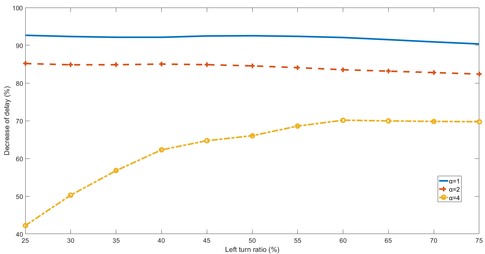
The delays of the LAF control and the ALAF control with different demand structures are tested. The results are shown in Fig. 12a. The delay of the ALAF control will increase with the growth of the traffic demand and let-turning ratio. In contrast, the delay of the LAF control is not sensitive to the left-turn ratio. That is because that the left-turn vehicles have a shorter shortest path and less conflict points on the path as shown as the vehicle $\omega_{1}$ in Fig. 1. In other words, the left-turn vehicles can be equivalent to right-turn vehicles under the LAF control. The decreases of delays by using the LAF control instead of the ALAF control under different demand structures are shown as Fig. 12b. Under all tested demand structures, at least 40 percent delay can be saved. The decrease of delay is dropped with the increase of traffic demand. When traffic demands are low and medium level, more than 90 and 80 percent delay can be saved, respectively. In contrast, the decrease delays are lower than 70 percent under the high level traffic demand. As for the influence of the left-turn ratio, the decrease of delays is not sensitive to the left-turn ratio when traffic demand is low level or medium level. On the contrary, the decrease of delay is growth from 40 percent to 70 percent with the increase of the left-turn ratio when the traffic demand is high level. The LAF control is more suitable to be used in intersections with large traffic demand and a large left-turn ratio or intersections with low traffic demand.

(a)

(b)

Figure 12: Simulation results of delay: (a) Delays of ALAF control and LAF control; (b) Decrease of Delay by using LAF.

However, the throughput of the LAF control and the ALAF control are still very similar with each other under different traffic condition as shown in 13a. Since the tested demands are lower than capacity, the throughput is close to tested demands. And the throughput is not changed with the increase of left-turn ratio. The comparison of throughput under the LAF control and the ALAF control is shown in Fig.13b. The gap between the LAF control and the ALAF control becomes larger with the growth of the traffic demand. But the throughput difference between two control methods can almost be neglected compared with the throughput which is changing from 770 veh/h to 3080 veh/h.

(a)

(b)

Figure 13: Improvement of Throughput by using LAF: (a) Throughput of ALAF and LAF; (b) Improvement of Throughput by using LAF.

For better exploring the improvement of capacity by using the LAF control and the ALAF control, higher demands are tested. The result is shown in Fig.14. Since the gap between the delay of the vehicle-actuated control and the delay of the LAF/ALAF control is large, the delay of the vehicle-actuated control is not shown in this figure for a better observation of the delays of the LAF control and the ALAF control. Under any demand level, the LAF control has a lower delay than the ALAF control.

Figure 14: Simulation results: vehicle throughput.

As for the throughput, the throughput of the vehicle-actuated control is hard to growth with the increase of the traffic demand after exceeding 2700 veh/h. In contrast, this situation of the ALAF control and the LAF control occurred at the value of around 3800 veh/h and 4200 veh/h, respectively. The capacity is improved after applying the LAF control and can reach 4200 veh/h. The ALAF control can also improve the capacity but is less significant than LAF control. The LAF control has better performance than the ALAF control not only on the delay but also on the throughput.

The advantages mainly come from two factors: 1) The relaxed constraints of defining approaching and exit lanes. Each lane can be used as both approaching and exit lane as long as safety is guaranteed. As a result, the spatial resources at the intersection can be utilized in a more effective way. 2) Flexible routing. Vehicles will take a detour by way of multiple arms to pass through the intersection if less delay can be achieved. In this way, the solution space of the vehicle trajectory planning is enlarged and potential better solutions are expected.

5.3.2 Temporal safety gaps

The signal-free management method is used in the LAF control and the ALAF control. It means the temporal safety gap is a critical parameter. Because temporal safety gap can influence control efficiency and safety significantly. Smaller temporal safety gaps may lead to a lower delay, but result in safety problems. The influence of temporal safety gaps on the performance of the LAF control and the ALAF control is investigated. 0.5 s is the smallest safety gap for constant time headway policy of all connected and automated vehicles environment and is selected as basic parameter by Bian et al. (2019) in their research. As for regular vehicles, the time headway will increase with the decrease of speed. The time headway is distributed centered on 2.5 s when the speed is between 3 m/s and 5 m/s (Li et al. (2010)). Since the smallest intersection passing speed in this case is 6 m/s which is larger than 5 m/s, the most common time headway should be lower than 2.5 s when the vehicles are regular vehicles. So the different values of temporal safety gaps are tested from 0.5 s to 2.5 s per 0.5 s. The result is shown in Fig. 15. The delays under both control methods increase with the growth of temporal safety gaps. The delay of the ALAF control is larger than the delay of the LAF control with any temporal safety gap. Except that, the ALAF control also has higher rising speed when the temporal safety gap is lower than 2 s. In other words, the ALAF control is more sensitive to the change of the temporal safety gap than the LAF control when time headway is lower than 2 s.

Figure 15: Sensitivity analysis of temporal safety gaps.

6 Conclusions and recommendations

This paper proposes an MILP model to optimize vehicle trajectories at a “signal-free” intersection without lane allocation under the fully CAV environment. Each lane can be used as both approaching and exit lanes for all vehicle movements including left-turn, through, and right-turn. Vehicle can take flexible routes by way of multiple arms to pass throughput the intersection. The interactions between vehicle trajectories are modeled explicitly at the microscopic level. Car-following and lane-changing behaviors of the vehicles within the control zone can be optimized in one unified framework in terms of total vehicle delay. In the implementation procedure, the planning horizon is adaptively adjusted to make a balance between the feasibility of the MILP model and computational efficiency. In the numerical studies, only the trajectories of newly arrived vehicles are optimized for computational efficiency at the cost of system optimality. The simulation results show that the proposed LAF control outperforms the vehicle-actuated control and the ALAF control in the previous study (Yu et al., 2019a) in terms of both vehicle delay and throughput. The sensitivity analysis further validates the advantages of the LAF control over the ALAF control with different demand structures and temporal safety gaps.

This study assumes a fully CAV environment. However, regular vehicles, CVs, and CAVs will coexist in the near future. It is worthwhile to investigate the control methods under the mixed traffic environment. This study focuses on isolated intersections. It is planned to extend the proposed model to a corridor and a network. For simplicity, the first-order vehicle dynamics models are used in this paper. It is not difficult to apply higher-order vehicle dynamics models but the model will be no longer linear. The solving algorithms could be a great challenge. The computational burden is heavy due to the large dimensions of the model, especially, when the trajectories of all vehicles are optimized at the same time. Efficient algorithms are expected to balance the solution quality and the computational time. Issues such as communication delays and detection issues may be inevitable even when 100% CAVs are deployed. Robust planning of vehicle trajectories is another research direction.

References

- Allsop (1976) Richard E. Allsop. SIGCAP: A computer program for assessing the traffic capacity of signal-controlled road junctions. Traffic Engineering & Control, 17(8-9):338–341, 1976. URL https://www.scopus.com/inward/record.uri?eid=2-s2.0-0016986186&partnerID=40&md5=e49ea20eeb87a2204774011ead5ffc86.
- Alonso et al. (2011) Javier Alonso, Vicente Milanés, Joshué Pérez, Enrique Onieva, Carlos González, and Teresa de Pedro. Autonomous vehicle control systems for safe crossroads. Transportation Research Part C: Emerging Technologies, 19(6):1095–1110, 2011. ISSN 0968-090X. doi: http://dx.doi.org/10.1016/j.trc.2011.06.002. URL http://www.sciencedirect.com/science/article/pii/S0968090X11000921.
- Au and Stone (2010) Tsz-Chiu Au and Peter Stone. Motion planning algorithms for autonomous intersection management. In Bridging the Gap Between Task and Motion Planning, Papers from the 2010 AAAI Workshop, Atlanta, Georgia, USA, July 11, 2010, volume WS-10-01 of AAAI Workshops. AAAI, 2010. URL http://aaai.org/ocs/index.php/WS/AAAIW10/paper/view/2053.
- Bian et al. (2019) Yougang Bian, Yang Zheng, Wei Ren, Shengbo Eben Li, Jianqiang Wang, and Keqiang Li. Reducing time headway for platooning of connected vehicles via V2V communication. Transportation Research Part C: Emerging Technologies, 102:87–105, 2019. ISSN 0968-090X. doi: https://doi.org/10.1016/j.trc.2019.03.002. URL http://www.sciencedirect.com/science/article/pii/S0968090X18311197.
- Carlino et al. (2013) Dustin Carlino, Stephen D. Boyles, and Peter Stone. Auction-based autonomous intersection management. In Proc. 16th Int. IEEE Conf. Intelligent Transportation Systems (ITSC 2013), pages 529–534, October 2013. doi: 10.1109/ITSC.2013.6728285.
- Dresner and Stone (2004) Kurt Dresner and Peter Stone. Multiagent traffic management: a reservation-based intersection control mechanism. In Proc. Third Int. Joint Conf. Autonomous Agents and Multiagent Systems AAMAS 2004, pages 530–537, July 2004.
- Dresner and Stone (2008) Kurt Dresner and Peter Stone. A multiagent approach to autonomous intersection management. Journal of artificial intelligence research, 31:591–656, 2008.
- Feng et al. (2018a) Shuo Feng, Xingmin Wang, Haowei Sun, Yi Zhang, and Li Li. A better understanding of long-range temporal dependence of traffic flow time series. Physica A: Statistical Mechanics and its Applications, 492:639–650, 2018a.
- Feng et al. (2019) Shuo Feng, Yi Zhang, Shengbo Eben Li, Zhong Cao, Henry X. Liu, and Li Li. String stability for vehicular platoon control: Definitions and analysis methods. Annual Reviews in Control, 2019.
- Feng et al. (2015) Yiheng Feng, K. Larry Head, Shayan Khoshmagham, and Mehdi Zamanipour. A real-time adaptive signal control in a connected vehicle environment. Transportation Research Part C: Emerging Technologies, 55:460–473, 2015. ISSN 0968-090X. doi: 10.1016/j.trc.2015.01.007.
- Feng et al. (2018b) Yiheng Feng, Chunhui Yu, and Henry X. Liu. Spatiotemporal intersection control in a connected and automated vehicle environment. Transportation Research Part C: Emerging Technologies, 89:364–383, 2018b. ISSN 0968-090X. doi: https://doi.org/10.1016/j.trc.2018.02.001. URL http://www.sciencedirect.com/science/article/pii/S0968090X1830144X.
- Gradinescu et al. (2007) Victor Gradinescu, Cristian Gorgorin, Raluca Diaconescu, Valentin Cristea, and Liviu Iftode. Adaptive traffic lights using car-to-car communication. In IEEE 65th Vehicular Technology Conference, pages 21–25, Dublin, 2007. IEEE. ISBN 1550-2252. doi: 10.1109/VETECS.2007.17. URL https://ieeexplore.ieee.org/ielx5/4196544/4212428/04212445.pdf?tp=&arnumber=4212445&isnumber=4212428.
- Guler et al. (2014) S. Ilgin Guler, Monica Menendez, and Linus Meier. Using connected vehicle technology to improve the efficiency of intersections. Transportation Research Part C: Emerging Technologies, 46:121–131, 2014. ISSN 0968-090X. doi: 10.1016/j.trc.2014.05.008.
- Guo et al. (2019a) Qiangqiang Guo, Li Li, and Xuegang (Jeff) Ban. Urban traffic signal control with connected and automated vehicles: A survey. Transportation Research Part C: Emerging Technologies, 101:313–334, 2019a. ISSN 0968-090X. doi: https://doi.org/10.1016/j.trc.2019.01.026. URL http://www.sciencedirect.com/science/article/pii/S0968090X18311641.
- Guo et al. (2019b) Yi Guo, Jiaqi Ma, Chenfeng Xiong, Xiaopeng Li, Fang Zhou, and Wei Hao. Joint optimization of vehicle trajectories and intersection controllers with connected automated vehicles: Combined dynamic programming and shooting heuristic approach. Transportation Research Part C: Emerging Technologies, 98:54–72, 2019b. ISSN 0968-090X. doi: https://doi.org/10.1016/j.trc.2018.11.010. URL http://www.sciencedirect.com/science/article/pii/S0968090X18303279.
- Gurobi Optimization, Inc. (2019) Gurobi Optimization, Inc. Gurobi optimizer reference manual, 2019. URL: http://www.gurobi.com/.
- Han and Gayah (2015) Ke Han and Vikash V. Gayah. Continuum signalized junction model for dynamic traffic networks: Offset, spillback, and multiple signal phases. Transportation Research Part B: Methodological, 77:213–239, 2015. ISSN 0191-2615. doi: https://doi.org/10.1016/j.trb.2015.03.005. URL http://www.sciencedirect.com/science/article/pii/S019126151500048X.
- Han et al. (2014) Ke Han, Vikash V. Gayah, Benedetto Piccoli, Terry L. Friesz, and Tao Yao. On the continuum approximation of the on-and-off signal control on dynamic traffic networks. Transportation Research Part B: Methodological, 61:73–97, 2014. ISSN 0191-2615. doi: https://doi.org/10.1016/j.trb.2014.01.001. URL http://www.sciencedirect.com/science/article/pii/S0191261514000022.
- He et al. (2012) Qing He, K. Larry Head, and Jun Ding. PAMSCOD: Platoon-based arterial multi-modal signal control with online data. Transportation Research Part C: Emerging Technologies, 20(1):164–184, 2012. ISSN 0968-090X. doi: http://dx.doi.org/10.1016/j.trc.2011.05.007. URL http://www.sciencedirect.com/science/article/pii/S0968090X11000775.
- Heydecker (1992) Benjamin Heydecker. Sequencing of traffic signals. Mathematics in transport planning and control. Clarendon Press, Oxford, 1992.
- Joyoung Lee (2012) Byungkyu Park Joyoung Lee. Development and evaluation of a cooperative vehicle intersection control algorithm under the connected vehicles environment. IEEE Transactions on Intelligent Transportation Systems, 13(1):81–90, March 2012. ISSN 1524-9050. doi: 10.1109/TITS.2011.2178836.
- Kamal et al. (2013) Md. Abdus Samad Kamal, Masakazu Mukai, Junichi Murata, and Taketoshi Kawabe. Model predictive control of vehicles on urban roads for improved fuel economy. IEEE Transactions on Control Systems Technology, 21(3):831–841, May 2013. ISSN 1063-6536. doi: 10.1109/TCST.2012.2198478.
- Kamalanathsharma and Rakha (2013) Raj Kishore Kamalanathsharma and Hesham A. Rakha. Multi-stage dynamic programming algorithm for eco-speed control at traffic signalized intersections. In 16th International IEEE Conference on Intelligent Transportation Systems (ITSC 2013), pages 2094–2099, Oct 2013. doi: 10.1109/ITSC.2013.6728538.
- Koonce et al. (2008) Peter Koonce, Lee Rodegerdts, Kevin Lee, Shaun Quayle, Scott Beaird, Cade Braud, Jim Bonneson, Phil Tarnoff, and Tom Urbanik. Traffic signal timing manual. Technical Report FHWA-HOP-08-024, Federal Highway Administration, Washington, DC, USA, Jun 2008. URL https://rosap.ntl.bts.gov/view/dot/20661. Tech Report.
- Krajzewicz et al. (2012) Daniel Krajzewicz, Jakob Erdmann, Michael Behrisch, and Laura Bieker. Recent development and applications of SUMO - Simulation of Urban MObility. International Journal On Advances in Systems and Measurements, 5(3&4):128–138, 2012.
- Levin et al. (2016) Michael W. Levin, Stephen D. Boyles, and Rahul Patel. Paradoxes of reservation-based intersection controls in traffic networks. Transportation Research Part A: Policy and Practice, 90:14–25, 2016. ISSN 0965-8564. doi: https://doi.org/10.1016/j.tra.2016.05.013. URL http://www.sciencedirect.com/science/article/pii/S0965856416303822.
- Li et al. (2010) Li Li, Fa Wang, Rui Jiang, Jian-Ming Hu, and Yan Ji. A new car-following model yielding log-normal type headways distributions. Chinese Physics B, 19(2):020513 (6 pp.) –, 2010. ISSN 1674-1056. URL http://dx.doi.org/10.1088/1674-1056/19/2/020513. car following model;log-normal type headways distributions;vehicles;traffic flow research field;vehicle dynamics;Galton board;time headway distributions;.
- Li et al. (2014a) Li Li, Ding Wen, and Danya Yao. A survey of traffic control with vehicular communications. IEEE Transactions on Intelligent Transportation Systems, 15(1):425–432, February 2014a. ISSN 1524-9050. doi: 10.1109/TITS.2013.2277737.
- Li et al. (2019) Zhenning Li, Qiong Wu, Hao Yu, Cong Chen, Guohui Zhang, Zong Z. Tian, and Panos D. Prevedouros. Temporal-spatial dimension extension-based intersection control formulation for connected and autonomous vehicle systems. Transportation Research Part C: Emerging Technologies, 104:234–248, 2019. ISSN 0968-090X. doi: https://doi.org/10.1016/j.trc.2019.05.003. URL http://www.sciencedirect.com/science/article/pii/S0968090X18305436.
- Li et al. (2013) Zhixia Li, Madhav V. Chitturi, Dongxi Zheng, Andrea R. Bill, and David A. Noyce. Modeling reservation-based autonomous intersection control in VISSIM. Transportation Research Record: Journal of the Transportation Research Board, 2381:81–90, 2013. ISSN 0361-1981. doi: 10.3141/2381-10.
- Li et al. (2014b) Zhuofei Li, Lily Elefteriadou, and Sanjay Ranka. Signal control optimization for automated vehicles at isolated signalized intersections. Transportation Research Part C: Emerging Technologies, 49:1–18, 2014b. ISSN 0968-090X. doi: 10.1016/j.trc.2014.10.001.
- Liang et al. (2018) Xiao (Joyce) Liang, S. Ilgin Guler, and Vikash V. Gayah. Signal timing optimization with connected vehicle technology: platooning to improve computational efficiency. Transportation Research Record, 2672(18):81–92, 2018. doi: 10.1177/0361198118786842. URL https://doi.org/10.1177/0361198118786842.
- Little et al. (1981) John D. C. Little, Mark D. Kelson, and Nathan H. Gartner. MAXBAND: A program for setting signals on arteries and triangular networks. Transportation Research Record: Journal of the Transportation Research Board, 795:40–46, 1981. ISSN 0309032091.
- Liu et al. (2019) Meiqi Liu, Meng Wang, and Serge Hoogendoorn. Optimal platoon trajectory planning approach at arterials. Transportation Research Record, page 0361198119847474, 2019.
- Liu and Smith (2015) Ronghui Liu and Mike Smith. Route choice and traffic signal control: A study of the stability and instability of a new dynamical model of route choice and traffic signal control. Transportation Research Part B: Methodological, 77:123–145, 2015. ISSN 0191-2615. doi: http://dx.doi.org/10.1016/j.trb.2015.03.012. URL http://www.sciencedirect.com/science/article/pii/S0191261515000557.
- Memoli et al. (2017) Silvio Memoli, Giulio E. Cantarella, Stefano de Luca, and Roberta Di Pace. Network signal setting design with stage sequence optimisation. Transportation Research Part B: Methodological, 100:20–42, 2017. ISSN 0191-2615. doi: https://doi.org/10.1016/j.trb.2017.01.013. URL http://www.sciencedirect.com/science/article/pii/S0191261516302363.
- Mirheli et al. (2019) Amir Mirheli, Mehrdad Tajalli, Leila Hajibabai, and Ali Hajbabaie. A consensus-based distributed trajectory control in a signal-free intersection. Transportation Research Part C: Emerging Technologies, 100:161–176, 2019. ISSN 0968-090X. doi: https://doi.org/10.1016/j.trc.2019.01.004. URL http://www.sciencedirect.com/science/article/pii/S0968090X18311343.
- Mitrovic et al. (2020) Nikola Mitrovic, Igor Dakic, and Aleksandar Stevanovic. Combined alternate-direction lane assignment and Reservation-Based intersection control. IEEE Transactions on Intelligent Transportation Systems, 21(4):1779–1789, 2020.
- Mohajerpoor et al. (2019) Reza Mohajerpoor, Meead Saberi, and Mohsen Ramezani. Analytical derivation of the optimal traffic signal timing: Minimizing delay variability and spillback probability for undersaturated intersections. Transportation Research Part B: Methodological, 119:45–68, 2019. ISSN 0191-2615. doi: https://doi.org/10.1016/j.trb.2018.11.004. URL http://www.sciencedirect.com/science/article/pii/S0191261518300201.
- Mohebifard and Hajbabaie (2019) Rasool Mohebifard and Ali Hajbabaie. Optimal network-level traffic signal control: A benders decomposition-based solution algorithm. Transportation Research Part B: Methodological, 121:252–274, 2019. ISSN 0191-2615. doi: https://doi.org/10.1016/j.trb.2019.01.012. URL http://www.sciencedirect.com/science/article/pii/S0191261518307616.
- Newell (2002) Gordon F. Newell. A simplified car-following theory: a lower order model. Transportation Research Part B: Methodological, 36(3):195–205, 2002. ISSN 0191-2615. doi: http://dx.doi.org/10.1016/S0191-2615(00)00044-8. URL http://www.sciencedirect.com/science/article/pii/S0191261500000448.
- Papageorgiou et al. (2003) Markos Papageorgiou, Christina Diakaki, Vaya Dinopoulou, Apostolos Kotsialos, and Yibing Wang. Review of road traffic control strategies. Proceedings of the IEEE, 91(12):2043–2067, 2003. ISSN 0018-9219. doi: 10.1109/JPROC.2003.819610.
- Pei et al. (2019) Huaxin Pei, Shuo Feng, Yi Zhang, and Danya Yao. A cooperative driving strategy for merging at on-ramps based on dynamic programming. IEEE Transactions on Vehicular Technology, 2019.
- Qian et al. (2019) Bo Qian, Haibo Zhou, Feng Lyu, Jinglin Li, Ting Ma, and Fen Hou. Toward collision-free and efficient coordination for automated vehicles at unsignalized intersection. IEEE Internet of Things Journal, 6(6):10408–10420, 2019.
- Sun et al. (2017) Weili Sun, Jianfeng Zheng, and Henry X. Liu. A capacity maximization scheme for intersection management with automated vehicles. Transportation Research Part C: Emerging Technologies, 23:121–136, 2017.
- Tachet et al. (2016) Remi Tachet, Stanislav Santi, Paolo andD Sobolevsky, Luis Ignacio Reyes-Castro, Emilio Frazzoli, Dirk Helbing, and Carlo Ratti. Revisiting street intersections using slot-based systems. PLOS ONE, 11(3):1–9, 03 2016. doi: 10.1371/journal.pone.0149607. URL https://doi.org/10.1371/journal.pone.0149607.
- Transportation Research Board (2010) (TRB) Transportation Research Board (TRB). HCM 2010: Highway Capacity Manual. Transportation Research Board, Washington, D.C., 2010.
- Ubiergo and Jin (2016) Gerard Aguilar Ubiergo and Wen-Long Jin. Mobility and environment improvement of signalized networks through Vehicle-to-Infrastructure (V2I) communications. Transportation Research Part C: Emerging Technologies, 68:70–82, 2016. ISSN 0968-090X. doi: https://doi.org/10.1016/j.trc.2016.03.010. URL http://www.sciencedirect.com/science/article/pii/S0968090X16300031.
- Wan et al. (2016) Nianfeng Wan, Ardalan Vahidi, and Andre Luckow. Optimal speed advisory for connected vehicles in arterial roads and the impact on mixed traffic. Transportation Research Part C: Emerging Technologies, 69:548–563, 2016. ISSN 0968-090X. doi: https://doi.org/10.1016/j.trc.2016.01.011. URL http://www.sciencedirect.com/science/article/pii/S0968090X16000292.
- Wang et al. (2014a) Meng Wang, Winnie Daamen, Serge P. Hoogendoorn, and Bart van Arem. Rolling horizon control framework for driver assistance systems. Part I: Mathematical formulation and non-cooperative systems. Transportation Research Part C: Emerging Technologies, 40:271–289, 2014a. ISSN 0968-090X. doi: https://doi.org/10.1016/j.trc.2013.11.023. URL http://www.sciencedirect.com/science/article/pii/S0968090X13002593.
- Wang et al. (2014b) Meng Wang, Winnie Daamen, Serge P. Hoogendoorn, and Bart van Arem. Rolling horizon control framework for driver assistance systems. Part II: Cooperative sensing and cooperative control. Transportation Research Part C: Emerging Technologies, 40:290–311, 2014b. ISSN 0968-090X. doi: https://doi.org/10.1016/j.trc.2013.11.024. URL http://www.sciencedirect.com/science/article/pii/S0968090X13002611.
- Webster (1958) Fo Vo Webster. Traffic signal settings, volume 39 of Road Research Technical Paper. Her Majesty’s Stationery Office, London, England, 1958.
- Xu et al. (2018) Biao Xu, Shengbo Eben Li, Yougang Bian, Shen Li, Xuegang Jeff Ban, Jianqiang Wang, and Keqiang Li. Distributed conflict-free cooperation for multiple connected vehicles at unsignalized intersections. Transportation Research Part C: Emerging Technologies, 93:322–334, 2018. ISSN 0968-090X. doi: https://doi.org/10.1016/j.trc.2018.06.004. URL http://www.sciencedirect.com/science/article/pii/S0968090X18308246.
- Yang et al. (2017) Kaidi Yang, Nan Zheng, and Monica Menendez. Multi-scale perimeter control approach in a connected-vehicle environment. Transportation Research Procedia, 23:101–120, 2017. ISSN 2352-1465. doi: https://doi.org/10.1016/j.trpro.2017.05.007. URL http://www.sciencedirect.com/science/article/pii/S2352146517302843. Papers Selected for the 22nd International Symposium on Transportation and Traffic Theory Chicago, Illinois, USA, 24-26 July, 2017.
- Yu et al. (2018) Chunhui Yu, Yiheng Feng, Henry X. Liu, Wanjing Ma, and Xiaoguang Yang. Integrated optimization of traffic signals and vehicle trajectories at isolated urban intersections. Transportation Research Part B: Methodological, 112:89–112, 2018. ISSN 0191-2615. doi: https://doi.org/10.1016/j.trb.2018.04.007. URL https://www.sciencedirect.com/science/article/pii/S0191261517306215.
- Yu et al. (2019a) Chunhui Yu, Yiheng Feng, Henry X. Liu, Wanjing Ma, and Xiaoguang Yang. Corridor level cooperative trajectory optimization with connected and automated vehicles. Transportation Research Part C: Emerging Technologies, 105:405–421, 2019a. ISSN 0968-090X. doi: https://doi.org/10.1016/j.trc.2019.06.002. URL http://www.sciencedirect.com/science/article/pii/S0968090X18316103.
- Yu et al. (2019b) Chunhui Yu, Weili Sun, Henry X. Liu, and Xiaoguang Yang. Managing connected and automated vehicles at isolated intersections: From reservation- to optimization-based methods. Transportation Research Part B: Methodological, 122:416–435, 2019b. ISSN 0191-2615. doi: https://doi.org/10.1016/j.trb.2019.03.002. URL http://www.sciencedirect.com/science/article/pii/S0191261517309980.
- Zohdy and Rakha (2016) Ismail H. Zohdy and Hesham A. Rakha. Intersection management via vehicle connectivity: The intersection cooperative adaptive cruise control system concept. Journal of Intelligent Transportation Systems, 20(1):17–32, 2016. ISSN 1547-2450. doi: 10.1080/15472450.2014.889918. URL http://dx.doi.org/10.1080/15472450.2014.889918.