arXiv is now an independent nonprofit! Learn more
License: CC BY 4.0
arXiv:2007.02708v3 [math.OC] 27 Jun 2026

The dual approach to non-negative super-resolution:
perturbation analysis and 1\ell_{1} data fidelity

Stéphane Chrétien Laboratoire ERIC, Université Lyon 2, Bron, France Alan Turing Institute, London, UK Andrew Thompson National Physical Laboratory, Teddington, UK Bogdan Toader MRC Laboratory of Molecular Biology, Cambridge, UK
Abstract

We study the problem of super-resolution, where we recover the locations and weights of non-negative point sources from (potentially noisy) samples of their convolution with a Gaussian kernel. Previous work has shown that exact recovery is possible by minimising the total variation norm of the measure, and a practical way to achieve this is by solving the dual problem. In this paper, we study the stability of the solution with respect to the solution of the dual problem, both in the case of exact measurements and in the case of measurements with additive noise. In particular, we establish a relationship between perturbations in the dual variable and perturbations in the primal variable around the true solution and, in the case of inexact measurements, we derive a similar relationship between the additive noise and perturbations in the dual variable using an 1\ell_{1} data fidelity whose dual is box constrained. Our analysis is based on a quantitative version of the implicit function theorem.

1 Problem setup

In the study of non-negative super-resolution, the aim is to estimate a signal xx which consists of a number of point sources with unknown locations and non-negative magnitudes, from only a few measurements of the convolution of xx with a known convolution kernel ϕ\phi. This is a problem that arises in a number of applications, for example fluorescence microscopy [1], astronomy [2] or ultrasound imaging [3]. In such applications, the measurement device has a limited resolution and cannot distinguish between distinct point sources that are close to each other in the input signal xx. This is often modelled as a deconvolution problem with a Gaussian kernel.

Specifically, let xx be a non-negative measure on I=[0,1]I=[0,1] consisting of kk unknown non-negative point sources:

x=i=1kaiδti,x=\sum_{i=1}^{k}a_{i}\delta_{t_{i}},

with ai>0a_{i}>0, for all i=1,,ki=1,\ldots,k, and let yjy_{j} be the possibly noisy measurements obtained by sampling the convolution of xx with a known kernel ϕ\phi at locations sjs_{j}:

yj=Iϕ(tsj)x(dt)+wj=i=1kaiϕ(tisj)+wj,y_{j}=\int_{I}\phi(t-s_{j})x(\operatorname{d\!}t)+w_{j}=\sum_{i=1}^{k}a_{i}\phi(t_{i}-s_{j})+w_{j}, (1)

for all j=1,,mj=1,\ldots,m or, in vector notation:

y=i=1kaiΦ(ti)+w,y=\sum_{i=1}^{k}a_{i}\Phi(t_{i})+w, (2)

where

y\displaystyle y =[y1,,ym]T,\displaystyle=[y_{1},\ldots,y_{m}]^{T}, (3)
Φ(t)\displaystyle\Phi(t) =[ϕ(ts1),,ϕ(tsm)]T,\displaystyle=[\phi(t-s_{1}),\ldots,\phi(t-s_{m})]^{T}, (4)
w\displaystyle w =[w1,,wm]T.\displaystyle=[w_{1},\ldots,w_{m}]^{T}. (5)

Of particular interest is the case of the Gaussian kernel:

ϕ(t)=et2/σ2,\phi(t)=e^{-t^{2}/\sigma^{2}}, (6)

where σ\sigma is assumed to be known to the practitioner.

In the setting where the measurements yy are exact, namely when w=0w=0, the signal xx can be recovered by solving the following problem:

minx0xTVsubject toy=IΦ(t)x(dt),\min_{x\geq 0}\|x\|_{TV}\quad\text{subject to}\quad y=\int_{I}\Phi(t)x(\operatorname{d\!}t), (7)

where TV\|\cdot\|_{TV} is the Total Variation (TV) norm for Radon measures defined as

xTV\displaystyle\|x\|_{\mathrm{TV}} =sup{ψdx;ψC(I),ψ1}.\displaystyle=\sup\left\{\int\psi\mathrm{d}x;\quad\psi\in C(I),\|\psi\|_{\infty}\leqslant 1\right\}. (8)

When the measurements are corrupted by additive noise, we depart from the standard approach in the super-resolution literature relying on a least squares 2\ell_{2} data fidelity term, and solve instead an 1\ell_{1} minimisation problem:

minx0yIΦ(t)x(dt)1such thatxTVΠ,\min_{x\geq 0}\left\|y-\int_{I}\Phi(t)x(\operatorname{d\!}t)\right\|_{1}\quad\text{such that}\quad\|x\|_{TV}\leq\Pi, (9)

where Π\Pi plays the role of the regularisation parameter. While 1\ell_{1} is also natural for robustness [4], our motivation is structural, as we will clarify in Section 1.1 and Section 3.

In the context of problems (7) and (9), in this manuscript we give bounds on the errors in the source locations {ti}i=1k\{t_{i}\}_{i=1}^{k} and weights {ai}i=1k\{a_{i}\}_{i=1}^{k} as a function of the errors in the dual variable when solving the dual problem, which we then extend to the case when the measurements are corrupted by additive noise, where we give an exact dependence of the error in the dual variable on the level of noise. A subset of the results in this paper has been presented in the conference article [5].

The problem of super-resolution has been studied extensively in the literature since the seminal paper [6], which addressed the case of complex amplitudes. Since the original contributions of Candès and Fernandez-Granda, there have been numerous follow-up results such as the ones by Schiebinger et al. [7], Duval and Peyré [8], Denoyelle et al. [9], Bendory et al. [10], Azaïs et al. [11], Eftekhari et al. [12, 13], and, more recently, Kalra et al. [14], Gabet et al. [15], Poon and Peyré [16], and Carioni and Del Grande [17]. For instance, the authors of [7] consider the noiseless setting by taking real-valued samples of yy with a more general choice of ϕ\phi (such as a Gaussian) and also assume xx to be non-negative as in the present work. Their proposed approach again involves TV norm minimisation with linear constraints. Bendory et al. [10] consider ϕ\phi to be Gaussian or Cauchy, do not place sign assumptions on xx, and also analyse the TV norm minimisation with linear fidelity constraints for estimating xx from noiseless samples of yy.

1.1 Motivation: dual certificate and 1\ell_{1} data fidelity

A standard way to approach problem (7) is by considering its dual:

maxλmyTλsubject toλTΦ(t)1tI,\max_{\lambda\in\mathbb{R}^{m}}\;y^{T}\lambda\quad\text{subject to}\quad\lambda^{T}\Phi(t)\leq 1\quad\forall t\in I, (10)

which is a finite-dimensional problem with infinitely many constraints, known as a semi-infinite program (SIP).

Solving the dual problem for λ\lambda leads to the dual certificate, a function of the form q(s)=j=1mλjϕ(ssj)q(s)=\sum_{j=1}^{m}\lambda_{j}\phi(s-s_{j}) (defined in Section 2), whose global maximisers are the source locations {ti}i=1k\{t_{i}\}_{i=1}^{k}. The weights {ai}i=1k\{a_{i}\}_{i=1}^{k} are then found by solving a least squares problem using the measurements and the source locations. Using the idea of the dual certificate, our perturbation results are quite intuitive: the locations of the global maximisers of the dual certificate are perturbed when λ\lambda is perturbed, which leads to perturbed source locations tit_{i}. Providing a quantitative analysis of the recovery error as a function of the error in the dual solution is the first goal of the present work.

The second goal is to extend the perturbation analysis to the case when the measurements are corrupted by additive noise. To do this, we leverage the specific form of the dual problem (10) and its associated dual certificate, and consider the dual of the 1\ell_{1} minimisation problem in (9), derived in Appendix A:

maxβ>0λmβ(λTyΠ)subject toλTΦ(t)1,t[0,1]andλ1/β,\max_{\begin{subarray}{c}\beta>0\\ \lambda\in\mathbb{R}^{m}\end{subarray}}\beta\left(\lambda^{T}y-\Pi\right)\quad\text{subject to}\quad\lambda^{T}\Phi(t)\leq 1,\quad\forall t\in[0,1]\quad\text{and}\quad\|\lambda\|_{\infty}\leq 1/\beta, (11)

where the box constraint is a consequence of the 1\ell_{1} data term, as the convex conjugate of 1\|\cdot\|_{1} is the indicator of the \ell_{\infty} ball. Since we only need the maximiser λ\lambda of (11) (not the optimal value) to form the dual certificate q(s)q(s), and for any fixed β\beta the argmax over λ\lambda is unchanged by the positive scaling β\beta and the additive constant βΠ-\beta\Pi in the objective, we may treat β\beta (equivalently the box radius τ=1/β\tau=1/\beta) as the regularisation parameter and solve the argmax problem:

argmaxλmλTysubject toλTΦ(t)1,t[0,1]andλτ,\displaystyle\operatorname*{\arg\!\max}_{\lambda\in\mathbb{R}^{m}}\lambda^{T}y\quad\text{subject to}\quad\lambda^{T}\Phi(t)\leq 1,\quad\forall t\in[0,1]\quad\text{and}\quad\|\lambda\|_{\infty}\leq\tau, (12)

where τ=1/β\tau=1/\beta. This specific form of the dual makes the perturbation analysis tractable in the noisy setting, as we will see in Section 3.

Both dual problems (10) and (12) are in the same finite-dimensional, polyhedral family, which is amenable to efficient optimisation algorithms such as exchange methods [18] or sequential quadratic programming [19]. Furthermore, this formulation of the dual problems can also be solved using non-smooth optimisation algorithms such as bundle methods [20, 21] by incorporating the constraint λTΦ(t)1,tI\lambda^{T}\Phi(t)\leq 1,\forall t\in I into the objective function as a penalty term. For example, the noise-free dual (10) can be reformulated as

minλmyTλ+Cmax{sups(λTΦ(s)1),0},\min_{\lambda\in\mathbb{R}^{m}}-y^{T}\lambda+C\cdot\max\left\{\sup_{s}\left(\lambda^{T}\Phi(s)-1\right),0\right\}, (13)

for a penalty parameter CC, with only the additional box constraint on λ\lambda in the noisy case.

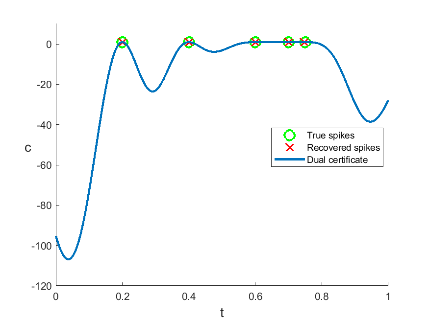
We briefly illustrate this approach by solving the noise-free dual problem (10) via (13) using the level bundle method, introduced in [20] to solve continuous sparse inverse problems. The level bundle method is applied to compute λ\lambda, and the spike locations are identified from the global maximisers of the resulting dual certificate. Figure 1(a) displays the recovered solution along with the corresponding dual certificate, showing that the method is able to recover the signal. Figure 1(b) shows the speed of convergence in terms of the decrease in the optimality gap (the model gap, see Appendix B), which is linear in practice.
Refer to caption
Refer to caption
Figure 1: A signal consisting of five spikes with locations {0.2,0.4,0.6,0.7,0.75}\{0.2,0.4,0.6,0.7,0.75\} and amplitude 11 is convolved with a Gaussian kernel ϕ(t)=et2/σ2\phi(t)=e^{-t^{2}/\sigma^{2}} with σ=0.1\sigma=0.1 and sampled at 1515 equispaced points on [0,1][0,1]. Then problem (13) is solved using the level bundle method. (a) Computed dual certificate and solution. (b) Decrease in optimality gap with iteration number.

1.2 Contributions

In this paper, we restrict our study to the case of Gaussian kernels. Our main results are:

  • When the measurements are exact, we provide bounds on how far the estimated spike locations tit_{i} and magnitudes aia_{i} are from their true values as the dual variable λ\lambda is perturbed from the optimal solution λ\lambda^{*} of (10). These bounds, given in Theorem 2 and Theorem 4, offer insight into the size of the error in the spike locations and magnitudes when the super-resolution problem is solved via its convex dual.

  • When the measurements are corrupted by additive noise, we leverage the connection between the convex dual of (7) and that of the 1\ell_{1} minimisation problem (9), highlighted in Section 1.1, to study the impact of measurement noise on the solution of the noisy dual problem (12). The main result is Theorem 8, where an explicit bound is given.

While the bounds given in these theorems apply only to the case when the convolution kernel is Gaussian, the same techniques can be applied to obtain perturbation bounds for other kernels, with a few differences in the way some sums in the proofs are bounded, which would be specific to the kernel used.

1.3 Comparison with previous work

1.3.1 Alternative formulations for the noiseless setting

For the particular case of non-negative xx, Boyd et al. [22] proposed an improved Frank-Wolfe algorithm in the primal. In certain instances, e.g. with Fourier samples (such as in [6, 23]), the dual, which is a SIP, can also be reformulated as a semi-definite program (SDP). From a practical point of view, SDP is notoriously slow for even a moderately large number of variables. The algorithm of [22] is a first order scheme with potential local correction steps, and is practically more viable.

As already mentioned, the main reason we advocate for using the dual problem (10) is that exact penalty can be used in order to reformulate the dual problem as a non-smooth minimisation problem for which methods such as bundle methods [20, 24] are efficient in practice. To the best of our knowledge, there is no analysis of the impact of obtaining approximate solutions of the dual on the quality of the recovered locations.

1.3.2 The penalised least squares approach

The approach adopted in [8, 9] is to solve a least-squares-type minimisation problem with a TV norm based penalty term (also referred to as the Beurling LASSO; see for example [25]) for recovering xx from samples of yy. The approach in [26] considers a natural finite approximation on the grid to the continuous problem, and studies the limiting behaviour as the grid becomes finer; see also [27]. These works develop a perturbation analysis which is different from ours since it applies to specific types of perturbations of a different problem (2\ell_{2} vs. 1\ell_{1} type fidelity terms), and does not provide precise quantitative dependencies with respect to all the parameters of the problem. Choosing the 1\ell_{1} fidelity enables the analysis in the noisy case presented in Section 3.

1.3.3 The Prony/Matrix Pencil approach

Another efficient approach is the one of [28] based on the original work of Hua and Sarkar [29] using a Matrix Pencil approach, extended to the multi-kernel setting in [30], and further investigated in [31, 32]. Perturbation analysis of the Matrix Pencil approach is provided in [28]; see also [30] for a more detailed exposition of these results with the correct order of dependencies. The reason we develop an analysis of the dual problem (10) here is that it easily extends to the multidimensional setting as well, at least for small dimensions. In contrast, the Matrix Pencil method, although very efficient in one dimension, becomes much more involved in several dimensions [33].

1.4 Plan of the paper

We start by presenting the noise-free perturbation results related to problem (10) in Section 2, followed by the perturbation results in the setting where the measurements are corrupted by noise in Section 3. The proofs of our results are given in Section 4 and we show numerical experiments to verify the validity of our results in practice in Section 5. Lastly, we conclude the paper in Section 6.

2 Bound on the error as λ\lambda is perturbed – the noise-free case

In this section we present our first main results, namely two theorems that give bounds on the perturbations around the source locations tit_{i} and the magnitudes aia_{i} respectively, as the dual variable is perturbed away from the optimiser λ\lambda^{*}, when the convolution kernel is a Gaussian with known width σ\sigma as defined in (6).

First, let us briefly give an informal statement of the main results in this section.

Informal Theorem.

(Stability of primal recovery) Let λm\lambda^{*}\in\mathbb{R}^{m} be a solution of the dual program (10) with ϕ\phi Gaussian and λ\lambda a perturbation of λ\lambda^{*} in a ball of radius δλ\delta_{\lambda}, given in Theorem 2 and let 𝐭,𝐚\mathbf{t}^{*},\mathbf{a^{*}} be the vectors of source locations and weights in the true signal xx and 𝐭~,𝐚~\mathbf{\tilde{t}},\mathbf{\tilde{a}} respectively their perturbations due to λ\lambda. Then, the error between 𝐭\mathbf{t^{*}} and 𝐭~\tilde{\mathbf{t}} is bounded by:

𝐭~𝐭2kCtλλ2.\|\mathbf{\tilde{t}}-\mathbf{t^{*}}\|_{2}\leq\sqrt{k}C_{t^{*}}\|\lambda-\lambda^{*}\|_{2}. (14)

Moreover, if the above error is bounded by δt\delta_{t}, given in Theorem 4, then the error between 𝐚\mathbf{a^{*}} and 𝐚~\tilde{\mathbf{a^{*}}} is bounded by:

𝐚~𝐚2Ca𝐭~𝐭2+O(𝐭~𝐭22).\|\mathbf{\tilde{a}}-\mathbf{a^{*}}\|_{2}\leq C_{a^{*}}\|\tilde{\mathbf{t}}-\mathbf{t^{*}}\|_{2}+O(\|\tilde{\mathbf{t}}-\mathbf{t^{*}}\|_{2}^{2}). (15)

As the two error bounds above are derived independently using different ideas, we will discuss them individually. Before giving the exact statement of each theorem, we define the concept of dual certificate, which plays an important role throughout this paper.

Definition 1.

(Dual certificate) Consider a solution λ\lambda^{*} of the dual problem (10) or (12). Then a dual certificate is a function of the form

q(t)=j=1mλjϕ(tsj)=λTΦ(t),q(t)=\sum_{j=1}^{m}\lambda_{j}^{*}\phi(t-s_{j})={\lambda^{*}}^{T}\Phi(t), (16)

which satisfies the conditions:

q(ti)=1,i=1,,k,\displaystyle q(t_{i})=1,\quad\forall i=1,\ldots,k, (17)
q(t)<1,tti,i=1,,k.\displaystyle q(t)<1,\quad\forall t\neq t_{i},\forall i=1,\ldots,k. (18)

The idea of dual certificate is common in the super-resolution literature, and we know that the global maximisers of q(t)q(t) correspond to the source locations {ti}i=1k\{t_{i}\}_{i=1}^{k} (see, for example [6, 7, 13], Once these are found, amplitudes {ai}i=1k\{a_{i}\}_{i=1}^{k} are obtained by solving a linear system.

We are now ready to discuss the perturbation results in the noise-free setting. In the following theorem, we consider the dual (10) of (7) and quantify how the source locations given by the global maximisers of the dual certificate formed by the dual solution λ\lambda^{*} are affected by perturbations of λ\lambda^{*}.

Theorem 2.

(Dependence of |tt||t-t^{*}| on λλ2\|\lambda-\lambda^{*}\|_{2}) Let λm\lambda^{*}\in\mathbb{R}^{m} be a solution of the dual program (10) with ϕ\phi Gaussian as given in (6) such that the the dual certificate q(s)q(s) defined in (16) satisfies conditions (17) and (18), λ\lambda a perturbation of λ\lambda^{*} in a ball of radius δλ\delta_{\lambda} and tt an arbitrary local maximiser of qλ(s)=j=1mλjϕ(ssj)q_{\lambda}(s)=\sum_{j=1}^{m}\lambda_{j}\phi(s-s_{j}). Note that, for λ=λ\lambda=\lambda^{*}, the corresponding local (and global) maximiser tt^{*} of qλ=qq_{\lambda^{*}}=q is a true source location in {ti}i=1k\{t_{i}\}_{i=1}^{k}. Let R=λ2σR=\frac{\|\lambda^{*}\|_{2}}{\sigma} and c3.9036c\approx 3.9036 a universal constant. If the radius δλ\delta_{\lambda} is bounded by

δλ|q′′(t)|2σ3e42(2+cR)m,\delta_{\lambda}\leq\frac{|q^{\prime\prime}(t^{*})|^{2}\sigma^{3}\sqrt{e}}{4\sqrt{2}\left(2+cR\right)m}, (19)

then

|tt|Ctλλ2,|t-t^{*}|\leq C_{t^{*}}\|\lambda-\lambda^{*}\|_{2}, (20)

where

Ct\displaystyle C_{t^{*}} =14+cR[1+22m(2+cR)|q′′(t)|e].\displaystyle=\frac{1}{4+cR}\left[1+\frac{2\sqrt{2m}(2+cR)}{|q^{\prime\prime}(t^{*})|\sqrt{e}}\right]. (21)
Proposition 3.

(Simplified CtC_{t^{*}}) Under the conditions of Theorem 2, the constant CtC_{t^{*}} can be further bounded by:

Ct<14+22em|q′′(t)|.C_{t^{*}}<\frac{1}{4}+\frac{2\sqrt{2}}{\sqrt{e}}\cdot\frac{\sqrt{m}}{|q^{\prime\prime}(t^{*})|}. (23)

The proofs of Theorem 2 and Proposition 3 are given in Section 4.1. As a brief summary, Theorem 2 is proved by applying the implicit function theorem to the function F(t,λ)=q(t)F(t,\lambda)=q^{\prime}(t), where q(t)q(t) is the dual certificate given in Definition 1, since we know that F(t,λ)=0F(t^{*},\lambda^{*})=0. This allows us to express tt as a function t(λ)t(\lambda) in a neighbourhood of (t,λ)(t^{*},\lambda^{*}), and a quantitative version of the theorem [34] gives an explicit expression for λt(λ)\partial_{\lambda}t(\lambda) and the neighbourhood in terms of the derivatives of FF. By bounding this derivative and the neighbourhood and then applying a truncated Taylor expansion to t(λ)t(\lambda), we obtain the result of Theorem 2.

One of the main conclusions which can be drawn from this result is that the primal spike location error is controlled in ll_{\infty}, but degrades as a function of the number of measurements in the order of m\sqrt{m}. Alternatively, we can write (20) in terms of the 2\ell_{2} norm of the error between the vector of true source locations 𝐭\mathbf{t^{*}} and the perturbed source locations 𝐭~\mathbf{\tilde{t}}:

𝐭~𝐭2kCtλλ2.\|\mathbf{\tilde{t}}-\mathbf{t^{*}}\|_{2}\leq\sqrt{k}C_{t^{*}}\|\lambda-\lambda^{*}\|_{2}.

Of crucial importance is the curvature of the dual certificate at the true solution: the flatter the certificate, the worse the estimation error. Our theorem also gives important information about the accuracy in the dual variable required to guarantee our upper bound on the error of recovery. This accuracy is of the inverse order of the number of measurements, which is quite a stringent constraint. Both the mm and the m\sqrt{m} factors are a consequence of the way we bound sums of shifted copies of the kernel, namely j=1mϕ(tsj)mmaxtϕ(t)\sum_{j=1}^{m}\phi(t-s_{j})\leq m\max_{t\in\mathbb{R}}\phi(t). Given the fast decay of the Gaussian, it is clear that this is not a tight bound. However, any bound would reflect the density of samples close to each source location.

We will now give a result regarding the perturbation of the magnitudes aia_{i} when λ\lambda^{*} is perturbed. Let Φ\Phi be the matrix whose entries are defined as

Φij=ϕ(tjsi),\Phi_{ij}=\phi(t_{j}-s_{i}), (24)

and 𝐭\mathbf{t^{*}} and 𝐚\mathbf{a^{*}} the vectors of source locations and weights:

𝐭=[t1,,tk]T,𝐚=[a1,,ak]T.\displaystyle\mathbf{t^{*}}=[t_{1},\ldots,t_{k}]^{T},\quad\quad\mathbf{a^{*}}=[a_{1},\ldots,a_{k}]^{T}.

When we solve (10) exactly, we obtain the source locations by finding the global maximisers of q(s)q(s). Then, the vector of weights 𝐚\mathbf{a^{*}} is found by solving the system

Φ𝐚=𝐲.\Phi\mathbf{a}=\mathbf{y}.

When the source locations are perturbed, we denote the resulting perturbed data matrix by:

Φ~=Φ+E,\tilde{\Phi}=\Phi+E, (25)

and we calculate the vector of perturbed weights 𝐚~\tilde{\mathbf{a}} as the solution of the least squares problem

min𝐚Φ~𝐚𝐲2.\min_{\mathbf{a}}\|\tilde{\Phi}\mathbf{a}-\mathbf{y}\|_{2}. (26)

The following theorem, proved in Section 4.2, gives a bound on the error 𝐚𝐚~2\|\mathbf{a^{*}}-\tilde{\mathbf{a}}\|_{2} between the vector of true weights 𝐚\mathbf{a^{*}} and the vector of weights 𝐚~\tilde{\mathbf{a}} obtained by solving the least squares problem (26) with the perturbed matrix Φ~\tilde{\Phi}, as a function of the error 𝐭~𝐭2\|\tilde{\mathbf{t}}-\mathbf{t^{*}}\|_{2} between the perturbed source locations 𝐭~\tilde{\mathbf{t}} and the true source locations 𝐭\mathbf{t^{*}}.

Theorem 4.

(Dependence of a~a2\|\mathbf{\tilde{a}}-\mathbf{a^{*}}\|_{2} on t~t2\|\mathbf{\tilde{t}}-\mathbf{t^{*}}\|_{2}) Let 𝐭[0,1]k\mathbf{t^{*}}\in[0,1]^{k} be the vector of true source locations, 𝐭~[0,1]k\tilde{\mathbf{t}}\in[0,1]^{k} the perturbed source locations in a ball of radius δt\delta_{t}, 𝐚\mathbf{a^{*}} the vector of true weights and 𝐚~\tilde{\mathbf{a}} the vector of perturbed weights obtained by solving problem (26). If the radius δt\delta_{t} is bounded by:

δt<σ2σmax(Φ)4e4/σ2m(1+σmin2(Φ)σmax2(Φ)1),\delta_{t}<\frac{\sigma^{2}\sigma_{\max}(\Phi)}{4e^{4/\sigma^{2}}\sqrt{m}}\left(\sqrt{1+\frac{\sigma_{\min}^{2}(\Phi)}{\sigma_{\max}^{2}(\Phi)}}-1\right), (27)

where σmax(Φ)\sigma_{\max}(\Phi), σmin(Φ)\sigma_{\min}(\Phi) are the largest and respectively smallest singular values of the matrix Φ\Phi defined in (24), then:

𝐚~𝐚2Cae4σ2maxj|t~jtj|𝐭~𝐭2+O(𝐭~𝐭22),\|\mathbf{\tilde{a}}-\mathbf{a^{*}}\|_{2}\leq C_{a^{*}}e^{\frac{4}{\sigma^{2}}\max_{j}|\tilde{t}_{j}-t_{j}|}\|\tilde{\mathbf{t}}-\mathbf{t^{*}}\|_{2}+O(\|\tilde{\mathbf{t}}-\mathbf{t^{*}}\|_{2}^{2}), (28)

where

Ca=4m𝐚2σ2σmin(Φ).C_{a^{*}}=\frac{4\sqrt{m}\|\mathbf{a^{*}}\|_{2}}{\sigma^{2}\sigma_{\min}(\Phi)}.

Note that we write the O(𝐭~𝐭22)O(\|\tilde{\mathbf{t}}-\mathbf{t^{*}}\|_{2}^{2}) term in the bound above in order to simplify the presentation of the result. We can, however, calculate the constants corresponding to the higher order terms in the bound by using the inequality (124) in the proof of Theorem 4 in Section 4.2. For example, the constant in the second order term is equal to Ca2/𝐚2[1+2σmax2(Φ)/σmin2(Φ)]C_{a^{*}}^{2}/\|\mathbf{a^{*}}\|_{2}\left[1+2\sigma^{2}_{\max}(\Phi)/\sigma^{2}_{\min}(\Phi)\right].

3 Bound on λλ2\|\lambda-\lambda^{*}\|_{2} in terms of the noise ww

In this section we assume that the measurements are corrupted by additive noise and we give a result where we bound the perturbation in the dual variable λ\lambda around the minimiser λ\lambda^{*} as a function of the noise ww in the measurements. Specifically, the noisy measurements are defined as in (1):

yj=Iϕj(t)x(dt)+wj=i=1kaiϕj(ti)+wj,y_{j}=\int_{I}\phi_{j}(t)x(\operatorname{d\!}t)+w_{j}=\sum_{i=1}^{k}a_{i}\phi_{j}(t_{i})+w_{j},

for wj0w_{j}\neq 0 and j=1,,mj=1,\ldots,m.

The aim is to estimate how the source locations {ti}i=1k\{t_{i}\}_{i=1}^{k} and weights {ai}i=1k\{a_{i}\}_{i=1}^{k} are affected by the additive noise ww in the measurements around the solution of the problem. In the previous section, we have established how the source locations and weights are perturbed around their true values as the dual variable λ\lambda is perturbed around its optimal value λ\lambda^{*}. In the noisy setting, we establish a quantitative relationship between the perturbations of λ\lambda around λ\lambda^{*} and the magnitude of the noise.

Before we state the main result, we first describe the exact mathematical setting under which the result holds. Then, we introduce the function F¯\bar{F} in (40) to which we apply the implicit function theorem, whose Jacobian is crucial for this result.

As discussed in Section 1.1, we consider the 1\ell_{1} minimisation problem (9) to account for noise in the measurements, and we focus on a particular form of its dual problem, given in (12), which we restate here:

argmaxλmyTλ\displaystyle\operatorname*{\arg\!\max}_{\lambda\in\mathbb{R}^{m}}y^{T}\lambda\quad such thatλTΦ(t)1,tI,\displaystyle\text{such that}\quad\lambda^{T}\Phi(t)\leq 1,\quad\forall t\in I,
andλτ,\displaystyle\quad\quad\text{and}\quad\|\lambda\|_{\infty}\leq\tau,

The parameter τ\tau is the inverse of the Lagrange multiplier corresponding to the constraint in (9), and therefore it plays the same regularisation role as Π\Pi (see Section 1.1 and Appendix A).

To motivate the exact form of the function F¯\bar{F} in (40) to which we apply the implicit function theorem to obtain the perturbation result from Theorem 8, consider the exact penalty formulation of (12):

argminλmΨΠ(λ)such thatλτ,\operatorname*{\arg\!\min}_{\lambda\in\mathbb{R}^{m}}\Psi_{\Pi}(\lambda)\quad\text{such that}\quad\|\lambda\|_{\infty}\leq\tau, (29)

where

ΨΠ(λ)=yTλ+Πmax{sups(j=1mλjϕ(ssj)1),0}.\Psi_{\Pi}(\lambda)=-y^{T}\lambda+\Pi\cdot\max\left\{\sup_{s}\left(\sum_{j=1}^{m}\lambda_{j}\phi(s-s_{j})-1\right),0\right\}. (30)

For a large enough value of Π\Pi, a solution to (29) which satisfies the constraints in (12) is also a solution of (12) (see, for example, Section 1.2 in [24]). This is a non-smooth optimisation problem and its solution can be found by using any method that relies on calculating subgradients, for example the level method [20].

A subgradient of ΨΠ(λ)\Psi_{\Pi}(\lambda) has the form:

ΨΠ={y+Πi=1kνig(si),(ν1++νk=1) if supsj=1mλjϕ(ssj)>1,y+Πi=1kνig(si),(ν1++νk1) if supsj=1mλjϕ(ssj)=1,y, if supsj=1mλjϕ(ssj)<1,\partial\Psi_{\Pi}=\begin{cases}-y+\Pi\sum_{i=1}^{k^{\prime}}\nu_{i}g(s_{i}^{*}),\quad(\nu_{1}+\ldots+\nu_{k^{\prime}}=1)&\quad\text{ if }\quad\sup_{s}\sum_{j=1}^{m}\lambda_{j}\phi(s-s_{j})>1,\\ -y+\Pi\sum_{i=1}^{k^{\prime}}\nu_{i}g(s_{i}^{*}),\quad(\nu_{1}+\ldots+\nu_{k^{\prime}}\leq 1)&\quad\text{ if }\quad\sup_{s}\sum_{j=1}^{m}\lambda_{j}\phi(s-s_{j})=1,\\ -y,&\quad\text{ if }\quad\sup_{s}\sum_{j=1}^{m}\lambda_{j}\phi(s-s_{j})<1,\end{cases} (31)

where {si}i=1k\{s_{i}^{*}\}_{i=1}^{k^{\prime}} are the global maximisers of the function j=1mλjϕ(ssj)\sum_{j=1}^{m}\lambda_{j}\phi(s-s_{j}), the vectors g(s)g(s) are of the form g(s)=[ϕ(ss1),,ϕ(ssm)]Tg(s)=[\phi(s-s_{1}),\ldots,\phi(s-s_{m})]^{T} and νi0\nu_{i}\geq 0 for all i=1,,ki=1,\ldots,k^{\prime}. Note that here we apply the formula for the subgradient of the max\max function and for the sup\sup function (see for example [24]). The coefficients in the convex combination from the formula for the subgradient of the max\max function with zero account for the case when ν1++νk<1\nu_{1}+\ldots+\nu_{k^{\prime}}<1111More specifically, both functions in the max\max attain their maximum, so we have that
Ψπ=y+Π[α1sups(j=1mλjϕ(ssj)1)+α20]\partial\Psi_{\pi}=-y+\Pi\left[\alpha_{1}\partial\sup_{s}\left(\sum_{j=1}^{m}\lambda_{j}\phi(s-s_{j})-1\right)+\alpha_{2}\partial 0\right], with α1,α2>0\alpha_{1},\alpha_{2}>0 and α1+α2=1\alpha_{1}+\alpha_{2}=1, and therefore Ψπ=y+Πi=1kα1νig(si)\partial\Psi_{\pi}=-y+\Pi\sum_{i=1}^{k^{\prime}}\alpha_{1}\nu_{i}^{\prime}g(s_{i}^{*}), with ν1++νk=1\nu_{1}^{\prime}+\ldots+\nu_{k^{\prime}}^{\prime}=1 and 0α110\leq\alpha_{1}\leq 1.
.

As in the noise-free setting, we assume here that the dual solution λ\lambda^{*} forms a dual certificate, namely the function q(s)q(s) as defined in (16) satisfies conditions (17) and (18). Then, the subdifferential at λ\lambda^{*} has the form:

ΨΠ(λ)=y+Πi=1kνig(ti),\partial\Psi_{\Pi}(\lambda^{*})=-y+\Pi\sum_{i=1}^{k}\nu_{i}g(t_{i}), (32)

where {ti}i=1k\{t_{i}\}_{i=1}^{k} are the source locations, so the optimality condition for (29):

0ΨΠ(λ),0\in\partial\Psi_{\Pi}(\lambda^{*}), (33)

is equivalent to:

y=Πi=1kνig(ti),y=\Pi\sum_{i=1}^{k}\nu_{i}g(t_{i}), (34)

for some ν1,,νk0\nu_{1},\ldots,\nu_{k}\geq 0 with ν1++νk1\nu_{1}+\ldots+\nu_{k}\leq 1 and for w=0w=0. Note that, given the definition of yy from (1), the optimality condition (34) is satisfied for

νi\displaystyle\nu_{i} =aiΠ,i=1,,k,\displaystyle=\frac{a_{i}}{\Pi},\quad\forall i=1,\ldots,k, (35)
wj\displaystyle w_{j} =0,j=1,,m,\displaystyle=0,\quad\forall j=1,\ldots,m, (36)

where in order to satisfy ν1++νk1\nu_{1}+\ldots+\nu_{k}\leq 1, we need Π\Pi such that:

Πa1++ai,\Pi\geq a_{1}+\ldots+a_{i}, (37)

which is the same as the constraint in (9).

Motivated by the above reasoning, we now apply the quantitative implicit function theorem, as given in [34], to a function FF of the form:

F([λ,ν]T,w)=i=1kaiΦ(ti)i=1kνiΦ(ti(λ))+w,F([\lambda,\nu]^{T},w)=\sum_{i=1}^{k}a_{i}\Phi(t_{i}^{*})-\sum_{i=1}^{k}\nu_{i}\Phi(t_{i}(\lambda))+w, (38)

where we know that F([λ,a]T,0)=0F([\lambda^{*},a]^{T},0)=0. For the sake of simplicity, we include the parameter Π\Pi in the coefficients νi\nu_{i}, so in the second sum in FF each νi\nu_{i} actually corresponds to Πνi\Pi\nu_{i}, and ν1++νkΠ\nu_{1}+\ldots+\nu_{k}\leq\Pi rather than ν1++νk1\nu_{1}+\ldots+\nu_{k}\leq 1.

However, note that F:m+k×mmF\mathrel{\mathop{\ordinarycolon}}\mathbb{R}^{m+k}\times\mathbb{R}^{m}\to\mathbb{R}^{m} and in order to apply the implicit function theorem to obtain the dependence of the first argument of FF as a function of the second argument, it is required that the spaces of the first argument, the second argument and the codomain of FF have the same dimension. To overcome this issue, we assume that the solution we work with has a few particular properties, since the dual certificate, given in Definition 1, is not unique in general. As before, we will assume that the solution λ\lambda^{*} to the dual problem (12) satisfies the dual certificate condition. In addition, we assume the existence of a solution λ¯\bar{\lambda}^{*} of (12) as follows:

Definition 5.

Let λm\lambda^{*}\in\mathbb{R}^{m} be a solution to the dual problem (12) with mkm-k entries on the boundary of the box constraint of (12) i.e. there exist indices γ1,,γmk{1,,m}\gamma_{1},\ldots,\gamma_{m-k}\in\{1,\ldots,m\} such that λγj=±τ\lambda^{*}_{\gamma_{j}}=\pm\tau, j=1,,mkj=1,\ldots,m-k. Then we define λ¯k\bar{\lambda}^{*}\in\mathbb{R}^{k} to be the vector that consists of the non-fixed entries of λ\lambda^{*}, in the same order, and λ¯k\bar{\lambda}\in\mathbb{R}^{k} a perturbation of λ¯\bar{\lambda}^{*}.

Remark.

In practice, such a solution λ¯\bar{\lambda}^{*} would be achieved due to the complementarity conditions at optimality corresponding to the box constraint λτ\|\lambda\|\leq\tau. This is a direct consequence of using an 1\ell_{1} data fidelity term in (9): an 2\ell_{2} fidelity term would instead give a Euclidean ball constraint (or a smooth quadratic dual term) and none of this complementarity.

Similarly, we define a vector consisting of 2k2k entries of Φ(t)\Phi(t) in (4).

Definition 6.

Let θ:={θ1,,θ2k}{1,,m}\theta\mathrel{\mathop{\ordinarycolon}}=\{\theta_{1},\ldots,\theta_{2k}\}\subset\{1,\ldots,m\}. Then we define Φ¯θ(t)\bar{\Phi}_{\theta}(t) to be the vector consisting of the entries of Φ(t)\Phi(t) in (4) corresponding to the indices in θ\theta:

Φ¯θ(t):=[ϕ(tsθ1),ϕ(tsθ2),,ϕ(tsθ2k)]T.\bar{\Phi}_{\theta}(t)\mathrel{\mathop{\ordinarycolon}}=[\phi(t-s_{\theta_{1}}),\phi(t-s_{\theta_{2}}),\ldots,\phi(t-s_{\theta_{2k}})]^{T}. (39)

We will also use Φ¯(t)\bar{\Phi}(t) to denote Φ¯θ(t)\bar{\Phi}_{\theta}(t) when the specific choice of θ\theta is not relevant in the context.

Lastly, given the definitions of λ¯\bar{\lambda} and Φ¯θ(t)\bar{\Phi}_{\theta}(t) above, we define the following function to which we will be able to apply the implicit function theorem:

Definition 7.

Let λm\lambda^{*}\in\mathbb{R}^{m} be a solution of (12) with mkm-k fixed entries and λ¯k\bar{\lambda}^{*}\in\mathbb{R}^{k} consisting of the non-fixed entries of λ\lambda^{*}, as given in Definition 5, and let Φ¯θ(t)\bar{\Phi}_{\theta}(t) be given as in Definition 6 for an index set θ\theta of 2k2k indices between 11 and mm. Then, for the perturbation λ¯\bar{\lambda} of λ¯\bar{\lambda}^{*}, we define the function F¯:2k×2k2k\bar{F}\mathrel{\mathop{\ordinarycolon}}\mathbb{R}^{2k}\times\mathbb{R}^{2k}\to\mathbb{R}^{2k} as:

F¯([λ¯,ν]T,wθ)=i=1kaiΦ¯θ(ti)i=1kνiΦ¯θ(ti(λ¯))+wθ,\bar{F}([\bar{\lambda},\nu]^{T},w_{\theta})=\sum_{i=1}^{k}a_{i}\bar{\Phi}_{\theta}(t_{i}^{*})-\sum_{i=1}^{k}\nu_{i}\bar{\Phi}_{\theta}(t_{i}(\bar{\lambda}))+w_{\theta}, (40)

where ti(λ¯)=tit_{i}(\bar{\lambda}^{*})=t_{i}^{*}, for i=1,,ki=1,\ldots,k, are the source locations corresponding to λ\lambda^{*} and wθ2kw_{\theta}\in\mathbb{R}^{2k} contains the entries of the noise vector wmw\in\mathbb{R}^{m} corresponding to the indices in θ\theta.

We can now state the main result of this section, namely a bound on the perturbation of λ\lambda^{*} (or more specifically λ¯\bar{\lambda}^{*}) as a function of the measurement noise. The proof is given in Section 4.3.

Theorem 8.

(Dependence of λλ2\|\lambda-\lambda^{*}\|_{2} on the noise ww) Let λm\lambda^{*}\in\mathbb{R}^{m} be a solution to the dual problem (12) with w=0w=0 , namely the optimal solution of (12) with noiseless measurements, which satisfies the conditions in Definition 5, and the vector λ¯k\bar{\lambda}^{*}\in\mathbb{R}^{k} of non-fixed entries of λ\lambda^{*}. For the function F¯\bar{F} in Definition 7, let JJ^{*} be its Jacobian with respect to the first variable, evaluated at ([λ¯,a]T,0)([\bar{\lambda}^{*},a]^{T},0) and σmin(J)\sigma_{\min}(J^{*}) its smallest singular value. We also assume that the solution λ\lambda^{*} forms a dual certificate, namely the function q(t)q(t) defined in (16) satisfies conditions (17) and (18). If JJ^{*} is invertible, w2δw\|w\|_{2}\leq\delta_{w} and

|q′′(t)|2(1+4mτσ2),|q^{\prime\prime}(t^{*})|\leq 2\left(1+\frac{4m\tau}{\sigma^{2}}\right), (41)

then, for a perturbation λ\lambda of λ\lambda^{*} with the same fixed entries to the boundary of the box constraint, we have that:

λλ2Cλw2,\left\|\lambda-\lambda^{*}\right\|_{2}\leq C_{\lambda^{*}}\cdot\left\|w\right\|_{2}, (42)

where

Cλ=2σmin(J),\displaystyle C_{\lambda^{*}}=\frac{2}{\sigma_{\min}(J^{*})}, (43)
δw=σmin(J)24P(m,k,σ,Π,τ,Ct),\displaystyle\delta_{w}=\frac{\sigma_{\min}(J^{*})^{2}}{4P(m,k,\sigma,\Pi,\tau,C_{t^{*}})}, (44)

and

P(\displaystyle P( m,k,σ,Π,τ,Ct)=2k[1σ2(2kCt2Π+4kCtΔ¯2τΠ)\displaystyle m,k,\sigma,\Pi,\tau,C_{t^{*}})=\sqrt{2}k\Bigg[\frac{1}{\sigma^{2}}\left(2\sqrt{k}C_{t^{*}}^{2}\Pi+4kC_{t^{*}}\bar{\Delta}_{2}\tau\Pi\right)
+1σ(2kCte+4kCt2Π+22Δ¯2Πe+8kCtΔ¯2τΠ+2kΔ¯2Πe+2eCt)],\displaystyle+\frac{1}{\sigma}\left(\frac{\sqrt{2k}C_{t^{*}}}{\sqrt{e}}+4\sqrt{k}C_{t^{*}}^{2}\Pi+\frac{2\sqrt{2}\bar{\Delta}_{2}\Pi}{\sqrt{e}}+8kC_{t^{*}}\bar{\Delta}_{2}\tau\Pi+\frac{\sqrt{2k}\bar{\Delta}_{2}\Pi}{\sqrt{e}}+\sqrt{\frac{2}{e}}C_{t^{*}}\right)\Bigg], (45)

where CtC_{t^{*}} is given in (21) in Theorem 2, c3.9036c\approx 3.9036, c2=4+c2e7.3484c_{2}=4+\frac{c\sqrt{2}}{\sqrt{e}}\approx 7.3484 are universal constants and

Δ¯2=kσ4(c2Ctmτ+22eσ).\bar{\Delta}_{2}=\frac{\sqrt{k}}{\sigma^{4}}\left(c_{2}C_{t^{*}}m\tau+\frac{2\sqrt{2}}{\sqrt{e}}\sigma\right). (46)

The theorem above makes explicit the dependence of the perturbation in the dual variable λ\lambda around the solution λ\lambda^{*} on the additive noise ww in the measurement vector yy, with the assumption given in Definition 5. This is a linear relation where the constant depends on the specific configuration of the problem we are solving, namely the locations and weights of the sources, and width of the Gaussian and the sampling locations. The theorem also gives an upper bound on the magnitude of the noise where this result holds as a function of the same parameters.

As an additional interpretation of Theorem 8 regarding the assumption on the fixed entries in λ\lambda and λ\lambda^{*}, it states that, for a solution λ\lambda to the dual problem (12) with noisy measurements that has mkm-k entries equal to the boundary of the box constraint, there is a solution λ\lambda^{*} to the noise-free dual problem w=0w=0 with the same entries fixed to the boundary of the box constraint and the error for the remaining kk entries bounded by (42).

Moreover, under a few additional assumptions, we give a simplified approximation of the constant PP in (45) for clarity:

Proposition 9.

(Simplified P) Under the conditions of Theorem 8 and, in addition, if Π,τ1\Pi,\tau\leq 1, then:

P(m,k,σ,Ct)=𝒪(mk5/2Ct2σ6).P(m,k,\sigma,C_{t^{*}})=\mathcal{O}\left(\frac{mk^{5/2}C_{t^{*}}^{2}}{\sigma^{6}}\right). (47)

One important observation is that, while the above result only applies to a subset of the entries in λ\lambda and ww, which entries are selected is not arbitrary. The choice of the entries in λ\lambda and ww reflects which samples sjs_{j} contain the most information, and therefore which noise entries in ww affect the solution to the optimisation problem the most. More specifically, in order for the Jacobian JJ^{*} to be invertible, we are led to select the samples (and therefore λ\lambda and ww entries) that satisfy this condition the best, namely the ones that are the closest to the source locations. We discuss this aspect in more detail in Section 3.1.

Lastly, note that the results in Section 2 and Section 3 refer to different optimisation problems: the duals (10) and (12) of problems (7) and (9) respectively. However, the proofs of our perturbation results rely on the property that the dual solution λ\lambda forms a dual certificate, the global maximisers of which give the locations of the point sources in the input signal xx, with the additional bound on λ\lambda from (12) being used in the proof of Theorem 8. Moreover, since our analysis is independent of the exact formulation of the primal problems, we conclude that the results from both Section 2 and Section 3 apply to the problem of super-resolution in the noisy setting, namely they give bounds of the perturbations of the source locations and weights as a consequence of noise in the measurements.

3.1 Discussion

One of the conditions in Theorem 8 is that the Jacobian JJ^{*} is invertible. While we do not provide a rigorous analysis of the conditions in which this is satisfied, in this section we discuss in more detail what the condition requires and give further motivation for why it is true in a reasonable scenario. Specifically, we assume that the samples that are used for calculating the Jacobian are the closest samples to the sources, i.e. the set θ\theta for which we define F¯\bar{F} in Definition 7 contains the two indices corresponding to the closest two samples to each source location, for each of the kk sources. Therefore, the rows in the system given by F¯\bar{F} in (40), as well as the entries in λ¯\bar{\lambda} and the entries in the noise vector wθw_{\theta}, correspond to these samples.

Recall that JJ^{*} is the Jacobian of the function F¯\bar{F} from (40) with respect to the first argument. The entries in JJ^{*} are:

λ¯lF¯([λ¯,ν]T,w)|λ¯=λ¯ν=awθ=0\displaystyle\partial_{\bar{\lambda}_{l}}\bar{F}([\bar{\lambda},\nu]^{T},w)\Bigr|_{\begin{subarray}{c}\bar{\lambda}=\bar{\lambda}^{*}\\ \nu=a\\ w_{\theta}=0\end{subarray}} =i=1kaiϕ(tisθj)λ¯lti(λ¯)\displaystyle=-\sum_{i=1}^{k}a_{i}\phi^{\prime}(t_{i}^{*}-s_{\theta_{j}})\partial_{\bar{\lambda}_{l}}t_{i}(\bar{\lambda}^{*}) (48)
=i=1kaiϕ(tisθj)ϕ(tisl)q′′(ti),\displaystyle=\sum_{i=1}^{k}\frac{a_{i}\phi^{\prime}(t_{i}^{*}-s_{\theta_{j}})\phi^{\prime}(t_{i}^{*}-s_{l})}{q^{\prime\prime}(t_{i}^{*})}, (49)

for l=1,,kl=1,\ldots,k, j=1,,2kj=1,\ldots,2k, where {sl}l=1k\{s_{l}\}_{l=1}^{k} correspond to the non-fixed entries of λ\lambda (i.e. λ¯\bar{\lambda}) and

νlF¯([λ¯,ν]T,wθ)|λ¯=λ¯ν=awθ=0=ϕ(tlsθj),\partial_{\nu_{l}}\bar{F}([\bar{\lambda},\nu]^{T},w_{\theta})\Bigr|_{\begin{subarray}{c}\bar{\lambda}=\bar{\lambda}^{*}\\ \nu=a\\ w_{\theta}=0\end{subarray}}=-\phi(t_{l}^{*}-s_{\theta_{j}}), (50)

for l=1,,kl=1,\ldots,k, j=1,,2kj=1,\ldots,2k, where in the first equality we used (60) with (64) and (65) plugged in, so the result holds under the conditions in Theorem 2, namely for λ\lambda with λλ2δλ\|\lambda-\lambda^{*}\|_{2}\leq\delta_{\lambda}, where δλ\delta_{\lambda} is given in (19).

Writing JJ^{*} as

J=[JλJν],J^{*}=[J_{\lambda}J_{\nu}], (51)

where the entries in the blocks JλJ_{\lambda} and JνJ_{\nu} are given by (49) and (50) respectively, we have that:

Jλ=i=1kaiq′′(ti)Φ¯(ti)Φ¯(ti)T,J_{\lambda}=\sum_{i=1}^{k}\frac{a_{i}}{q^{\prime\prime}(t_{i}^{*})}\bar{\Phi}^{\prime}(t_{i}^{*})\bar{\Phi}^{\prime}(t_{i}^{*})^{T}, (52)

and

Jν=[Φ¯(t1)Φ¯(tk)],J_{\nu}=-[\bar{\Phi}(t_{1}^{*})\ldots\bar{\Phi}(t_{k}^{*})], (53)

where

Φ¯(t)=[ϕ(tsθ1),,ϕ(tsθ2k)]T,\displaystyle\bar{\Phi}(t)=[\phi(t-s_{\theta_{1}}),\ldots,\phi(t-s_{\theta_{2k}})]^{T}, (54)
Φ¯(t)=[ϕ(tsθ1),,ϕ(tsθ2k)]T.\displaystyle\bar{\Phi}^{\prime}(t)=[\phi^{\prime}(t-s_{\theta_{1}}),\ldots,\phi^{\prime}(t-s_{\theta_{2k}})]^{T}. (55)

Note that rank(Jν)=krank(J_{\nu})=k by the T-systems property of the Gaussian (assuming that the t1tkt_{1}\leq\ldots\leq t_{k} and sθ1sθ2ks_{\theta_{1}}\leq\ldots\leq s_{\theta_{2k}}) and in order for the matrix JJ^{*} to be invertible we need rank(J)=2krank(J^{*})=2k, as it is a square matrix with 2k2k columns. By rewriting the columns of JλJ_{\lambda}, we have that:

J=[i=1kaiϕ(tis1)q′′(ti)Φ¯(ti)i=1kaiϕ(tisk)q′′(ti)Φ¯(ti)Φ¯(t1)Φ¯(tk)],\displaystyle J^{*}=\left[\sum_{i=1}^{k}\frac{a_{i}\phi^{\prime}(t_{i}^{*}-s_{1})}{q^{\prime\prime}(t_{i}^{*})}\bar{\Phi}^{\prime}(t_{i}^{*})\quad\ldots\quad\sum_{i=1}^{k}\frac{a_{i}\phi^{\prime}(t_{i}^{*}-s_{k})}{q^{\prime\prime}(t_{i}^{*})}\bar{\Phi}^{\prime}(t_{i}^{*})\quad-\bar{\Phi}(t_{1}^{*})\quad\ldots\quad-\bar{\Phi}(t_{k}^{*})\right], (56)

and by taking its determinant and using the multi-linearity property of the determinant with respect to its columns, we have that:

det(J)\displaystyle\det(J^{*}) =(1)ka1akq′′(t1)q′′(tk)\displaystyle=(-1)^{k}\frac{a_{1}\ldots a_{k}}{q^{\prime\prime}(t_{1}^{*})\ldots q^{\prime\prime}(t_{k}^{*})}
l=1k!(i=1kϕ(Pl(ti)si))|Pl(Φ¯(t1))Pl(Φ¯(tk))Φ¯(t1)Φ¯(tk)|,\displaystyle\cdot\sum_{l=1}^{k!}\left(\prod_{i=1}^{k}\phi^{\prime}(P_{l}(t_{i}^{*})-s_{i})\right)\left|P_{l}(\bar{\Phi}^{\prime}(t_{1}^{*}))\quad\ldots\quad P_{l}(\bar{\Phi}^{\prime}(t_{k}^{*}))\quad\bar{\Phi}(t_{1}^{*})\quad\ldots\quad\bar{\Phi}(t_{k}^{*})\right|, (57)

where PlP_{l} for l=1,,k!l=1,\ldots,k! are the permutations of kk elements. Note that when we expand the determinant, the terms in the final sum are determinants with all the possible combinations of the vectors in each sum, which results in most determinants having repeated columns, so they are equal to zero. The only non-zero determinants in the resulting sum are the ones where the first kk columns are the vectors {Φ(ti)}i=1k\{\Phi^{\prime}(t_{i}^{*})\}_{i=1}^{k} and their permutations, multiplied by the corresponding constants. We now order the columns of the determinant:

det(J)\displaystyle\det(J^{*}) =(1)ka1akq′′(t1)q′′(tk)\displaystyle=(-1)^{k}\frac{a_{1}\ldots a_{k}}{q^{\prime\prime}(t_{1}^{*})\ldots q^{\prime\prime}(t_{k}^{*})}
l=1k!sign(Pi)(i=1kϕ(Pl(ti)si))|Φ¯(t1)Φ¯(t1)Φ¯(tk)Φ¯(tk)|,\displaystyle\qquad\qquad\sum_{l=1}^{k!}sign(P_{i})\left(\prod_{i=1}^{k}\phi^{\prime}(P_{l}(t_{i}^{*})-s_{i})\right)\left|\bar{\Phi}(t_{1}^{*})\quad\bar{\Phi}^{\prime}(t_{1}^{*})\quad\ldots\quad\bar{\Phi}(t_{k}^{*})\quad\bar{\Phi}^{\prime}(t_{k}^{*})\right|,
=(1)ka1akq′′(t1)q′′(tk)|Φ¯(t1)Φ¯(t1)Φ¯(tk)Φ¯(tk)|\displaystyle=(-1)^{k}\frac{a_{1}\ldots a_{k}}{q^{\prime\prime}(t_{1}^{*})\ldots q^{\prime\prime}(t_{k}^{*})}\left|\bar{\Phi}(t_{1}^{*})\quad\bar{\Phi}^{\prime}(t_{1}^{*})\quad\ldots\quad\bar{\Phi}(t_{k}^{*})\quad\bar{\Phi}^{\prime}(t_{k}^{*})\right|
l=1k!sign(Pl)(i=1kϕ(Pl(ti)si)),\displaystyle\qquad\qquad\sum_{l=1}^{k!}sign(P_{l})\left(\prod_{i=1}^{k}\phi^{\prime}(P_{l}(t_{i}^{*})-s_{i})\right), (58)

where by sign(Pi)sign(P_{i}) we denote the sign of the determinant corresponding to the permutation PiP_{i} after reordering the columns as above. Because of the extended T-system property of the Gaussian function [35], the determinant above is strictly positive. The dominant term in the sum is the one corresponding to the identity permutation, where for each i=1,,ki=1,\ldots,k, the sample sis_{i} is the closest sample to the source location tit_{i}^{*}. As the samples get further, the terms of the sum approach zero. This can be expressed more quantitatively by imposing explicit conditions on the distances between the closest samples and the sources, the separation of sources and the separation of samples, as done, for example, in [13].

As a last remark to motivate the choice of the dimension of λ¯\bar{\lambda}^{*} and λ¯\bar{\lambda} in Definition 5, note the expansion in (57) of det(J)\det(J^{*}). If the vector λ¯\bar{\lambda} had more than kk entries, then the columns consisting of the permutations of Φ¯(ti)\bar{\Phi}^{\prime}(t_{i}^{*}) would inevitably be repeated, since there are kk sources tit_{i}^{*} and more than kk such columns. This implies that all the determinants in the sum would be zero and, therefore, JJ^{*} would not be invertible, implying that Theorem 8 would not be true in this case. This explains why choosing λ¯\bar{\lambda} to contain more than kk entries of λ\lambda would be incompatible with our analysis in the proof of Theorem 8.

4 Proofs

In this section we present the proofs of the theorems from Sections 2 and 3.

4.1 Proof of Theorem 2 (Dependence of |tt||t-t^{*}| on λλ2\|\lambda-\lambda^{*}\|_{2})

Let tt^{*} be an arbitrary local maximiser of the function q(t)q(t) in (16), so tt^{*} is also a source location, and λ\lambda^{*} the solution to (10). The key step in this proof is applying a quantitative version of the implicit function theorem [34] to the function:

F(t,λ)=j=1mλjϕ(tsj),F(t,\lambda)=\sum_{j=1}^{m}\lambda_{j}\phi^{\prime}(t-s_{j}), (59)

where F(t,λ)=0F(t^{*},\lambda^{*})=0 because tt^{*} is a maximizer of q(s)q(s) in (16). The theorem allows us to express tt as a function t(λ)t(\lambda) of λ\lambda with:

λt(λ)=[tF(t(λ),λ)]1λF(t(λ),λ),\partial_{\lambda}t(\lambda)=-\left[\partial_{t}F(t(\lambda),\lambda)\right]^{-1}\partial_{\lambda}F(t(\lambda),\lambda), (60)

for tt in a ball of radius δ0\delta_{0} around tt^{*} and for λ\lambda in a ball of radius δ1δ0\delta_{1}\leq\delta_{0} around λ\lambda^{*}, where δ0\delta_{0} is chosen such that

sup(t,λ)VδI[tF(t,λ)]1tF(t,λ)12,\sup_{(t,\lambda)\in V_{\delta}}\left\|I-\left[\partial_{t}F(t^{*},\lambda^{*})\right]^{-1}\partial_{t}F(t,\lambda)\right\|\leq\frac{1}{2}, (61)

where Vδ={(t,λ)m+1:|tt|δ0,λλδ0}V_{\delta}=\left\{(t,\lambda)\in\mathbb{R}^{m+1}\mathrel{\mathop{\ordinarycolon}}|t-t^{*}|\leq\delta_{0},\|\lambda-\lambda^{*}\|\leq\delta_{0}\right\} and δ1\delta_{1} is given by

δ1=(2MtBλ)1δ0,\delta_{1}=(2M_{t}B_{\lambda})^{-1}\delta_{0}, (62)

where

Bλ\displaystyle B_{\lambda} =sup(t,λ)VδλF(t,λ)2,\displaystyle=\sup_{(t,\lambda)\in V_{\delta}}\|\partial_{\lambda}F(t,\lambda)\|_{2},
Mt\displaystyle M_{t} =tF(t,λ)12.\displaystyle=\left\|\partial_{t}F(t^{*},\lambda^{*})^{-1}\right\|_{2}.

The following two lemmas, proved in Sections 4.1.1 and 4.1.2 respectively, give us values of δ0\delta_{0} and δ1\delta_{1} that define balls around tt^{*} and λ\lambda^{*} respectively which are included in the balls required by the quantitative implicit function theorem with radii defined in (61) and (62).

Lemma 10.

(Radius of ball around tt^{*}) The condition (61) is satisfied if

δ0=σ2|q′′(t)|m(4+2cλ2σ).\delta_{0}=\frac{\sigma^{2}|q^{\prime\prime}(t^{*})|}{\sqrt{m}\left(4+2c\cdot\frac{\|\lambda^{*}\|_{2}}{\sigma}\right)}. (63)
Lemma 11.

(Radius of ball around λ\lambda^{*}) For δ0\delta_{0} from Lemma 63 and δ1\delta_{1} from condition (62), the following choice of δλ\delta_{\lambda}:

δλ=σe|q′′(t)|22mδ0\delta_{\lambda}=\frac{\sigma\sqrt{e}|q^{\prime\prime}(t^{*})|}{2\sqrt{2m}}\cdot\delta_{0}

satisfies δλ<δ1\delta_{\lambda}<\delta_{1}.

Given the definition of the function FF in (59), we have that

tF(t,λ)\displaystyle\partial_{t}F(t,\lambda) =j=1mλjϕ′′(tsj),\displaystyle=\sum_{j=1}^{m}\lambda_{j}\phi^{\prime\prime}(t-s_{j}), (64)
λF(t,λ)\displaystyle\partial_{\lambda}F(t,\lambda) =[ϕ(ts1),,ϕ(tsm)]T.\displaystyle=[\phi^{\prime}(t-s_{1}),\quad\ldots\quad,\phi^{\prime}(t-s_{m})]^{T}. (65)

By applying Taylor expansion to t(λ)t(\lambda) around λ\lambda^{*} in the region defined by δ0\delta_{0} and δλ\delta_{\lambda}, we have that

t(λ)=t(λ)+λλ,λt(λδ),t(\lambda)=t(\lambda^{*})+\left<\lambda-\lambda^{*},\partial_{\lambda}t(\lambda_{\delta})\right>,

for some λδ\lambda_{\delta} on the line segment determined by λ\lambda^{*} and λ\lambda, so

|t(λ)t(λ)|\displaystyle\left|t(\lambda)-t(\lambda^{*})\right| λλ2λt(λδ)2\displaystyle\leq\left\|\lambda-\lambda^{*}\right\|_{2}\cdot\left\|\partial_{\lambda}t(\lambda_{\delta})\right\|_{2}
δ0j=1mλδjϕ′′(t(λδ)sj)[ϕ(t(λδ)s1),,ϕ(t(λδ)sm)]2,\displaystyle\leq\frac{\delta_{0}}{\sum_{j=1}^{m}{\lambda_{\delta}}_{j}\phi^{\prime\prime}(t(\lambda_{\delta})-s_{j})}\cdot\left\|\left[\phi^{\prime}(t(\lambda_{\delta})-s_{1}),\quad\ldots\quad,\phi^{\prime}(t(\lambda_{\delta})-s_{m})\right]\right\|_{2}, (66)

where in the last inequality we used that λλδ0\|\lambda-\lambda^{*}\|\leq\delta_{0} and (60). We now need to bound the terms in (66) for the Gaussian kernel ϕ(t)=et2/σ2\phi(t)=e^{-t^{2}/\sigma^{2}}. First, we rewrite the last inequality as

|t(λ)t(λ)|\displaystyle|t(\lambda)-t(\lambda^{*})| j=1m(λδj+λjλj)ϕ′′(t(λδ)sj)\displaystyle\sum_{j=1}^{m}({\lambda_{\delta}}_{j}+\lambda_{j}^{*}-\lambda_{j}^{*})\phi^{\prime\prime}(t(\lambda_{\delta})-s_{j})
δ0[ϕ(t(λδ)s1),,ϕ(t(λδ)sm)]2,\displaystyle\leq\delta_{0}\cdot\left\|\left[\phi^{\prime}(t(\lambda_{\delta})-s_{1}),\quad\ldots\quad,\phi^{\prime}(t(\lambda_{\delta})-s_{m})\right]\right\|_{2}, (67)

we apply the reverse triangle inequality in the sum on the left hand side:

|t(λ)t(λ)|\displaystyle|t(\lambda)-t(\lambda^{*})| [|j=1m(λδjλj)ϕ′′(t(λδ)sj)|+|j=1mλjϕ′′(t(λδ)sj)|]\displaystyle\left[-\left|\sum_{j=1}^{m}({\lambda_{\delta}}_{j}-\lambda_{j}^{*})\phi^{\prime\prime}(t(\lambda_{\delta})-s_{j})\right|+\left|\sum_{j=1}^{m}\lambda_{j}^{*}\phi^{\prime\prime}(t(\lambda_{\delta})-s_{j})\right|\right]
δ0[ϕ(t(λδ)sj)]j=1m2\displaystyle\leq\delta_{0}\cdot\left\|\left[\phi^{\prime}(t(\lambda_{\delta})-s_{j})\right]_{j=1}^{m}\right\|_{2} (68)

and then we apply the Cauchy-Schwartz inequality to the first sum on the left hand side above to obtain:

|t(λ)t(λ)|\displaystyle|t(\lambda)-t(\lambda^{*})| [λδλ2[ϕ′′(t(λδ)sj)]j=1m2+|j=1mλjϕ′′(t(λδ)sj)|]\displaystyle\left[-\left\|\lambda_{\delta}-\lambda^{*}\right\|_{2}\cdot\left\|\left[\phi^{\prime\prime}(t(\lambda_{\delta})-s_{j})\right]_{j=1}^{m}\right\|_{2}+\left|\sum_{j=1}^{m}\lambda_{j}^{*}\phi^{\prime\prime}(t(\lambda_{\delta})-s_{j})\right|\right]
δ0[ϕ(t(λδ)sj)]j=1m2.\displaystyle\leq\delta_{0}\cdot\left\|\left[\phi^{\prime}(t(\lambda_{\delta})-s_{j})\right]_{j=1}^{m}\right\|_{2}. (69)

To simplify the notation, we write δt=|t(λ)t(λ)|\delta_{t}=|t(\lambda)-t(\lambda^{*})| and

A\displaystyle A =[ϕ′′(t(λδ)sj)]j=1m2,\displaystyle=\left\|\left[\phi^{\prime\prime}(t(\lambda_{\delta})-s_{j})\right]_{j=1}^{m}\right\|_{2}, (70)
B\displaystyle B =|j=1mλjϕ′′(t(λδ)sj)|,\displaystyle=\left|\sum_{j=1}^{m}\lambda_{j}^{*}\phi^{\prime\prime}(t(\lambda_{\delta})-s_{j})\right|, (71)
C\displaystyle C =[ϕ(t(λδ)sj)]j=1m2,\displaystyle=\left\|\left[\phi^{\prime}(t(\lambda_{\delta})-s_{j})\right]_{j=1}^{m}\right\|_{2}, (72)

and by using222Since λλδ0\|\lambda-\lambda^{*}\|\leq\delta_{0} and λδ\lambda_{\delta} is on the line segment between λ\lambda^{*} and λ\lambda, then λδ\lambda_{\delta} is in the ball centred at λ\lambda^{*} with radius δ0\delta_{0}. λδλ2δ0\|\lambda_{\delta}-\lambda^{*}\|_{2}\leq\delta_{0}, we have that:

δt(δ0A+B)δ0C,\delta_{t}(-\delta_{0}A+B)\leq\delta_{0}C, (73)

which can be further re-written as:

δtC+δtABδ0.\delta_{t}\leq\frac{C+\delta_{t}A}{B}\cdot\delta_{0}. (74)

The aim now is to obtain a bound on δt\delta_{t} as a function of δ0\delta_{0} and the parameters of the problem. Therefore, we need to lower bound BB and upper bound C+δtAC+\delta_{t}A.

Bounding A,B,C

We start with BB, for which we want to calculate a lower bound. First, we Taylor expand each term of the sum around t(λ)sjt(\lambda^{*})-s_{j} as follows:

B\displaystyle B =|j=1mλjϕ′′(t(λ)sj+t(λδ)t(λ))|\displaystyle=\left|\sum_{j=1}^{m}\lambda_{j}^{*}\phi^{\prime\prime}(t(\lambda^{*})-s_{j}+t(\lambda_{\delta})-t(\lambda^{*}))\right|
=|j=1mλjϕ′′(t(λ)sj)+(t(λδ)t(λ))j=1mλjϕ′′′(ξj)|\displaystyle=\left|\sum_{j=1}^{m}\lambda_{j}^{*}\phi^{\prime\prime}(t(\lambda^{*})-s_{j})+\left(t(\lambda_{\delta})-t(\lambda^{*})\right)\sum_{j=1}^{m}\lambda_{j}^{*}\phi^{\prime\prime\prime}(\xi_{j})\right| (75)
|j=1mλjϕ′′(t(λ)sj)||t(λδ)t(λ)||j=1mλjϕ′′′(ξj)|,\displaystyle\geq\left|\sum_{j=1}^{m}\lambda_{j}^{*}\phi^{\prime\prime}(t(\lambda^{*})-s_{j})\right|-\left|t(\lambda_{\delta})-t(\lambda^{*})\right|\left|\sum_{j=1}^{m}\lambda_{j}^{*}\phi^{\prime\prime\prime}(\xi_{j})\right|, (76)

where ξj[t(λ)sj|t(λδ)t(λ)|,t(λ)sj+|t(λδ)t(λ)|]\xi_{j}\in\left[t(\lambda^{*})-s_{j}-|t(\lambda_{\delta})-t(\lambda^{*})|,\quad t(\lambda^{*})-s_{j}+|t(\lambda_{\delta})-t(\lambda^{*})|\right] for j=1,,mj=1,\ldots,m, and on the last line we used the reverse triangle inequality. We calculate an upper bound of the last sum in the previous equation as follows:

|j=1mλjϕ′′′(ξj)|\displaystyle\left|\sum_{j=1}^{m}\lambda_{j}^{*}\phi^{\prime\prime\prime}(\xi_{j})\right| λ2[ϕ′′′(ξj)]j=1m2,by Cauchy-Schwartz,\displaystyle\leq\left\|\lambda^{*}\right\|_{2}\cdot\left\|\left[\phi^{\prime\prime\prime}(\xi_{j})\right]_{j=1}^{m}\right\|_{2},\quad\quad\text{by Cauchy-Schwartz,} (77)
cλ2mσ3,\displaystyle\leq\frac{c\|\lambda^{*}\|_{2}\sqrt{m}}{\sigma^{3}}, (78)

where in the last line we used the maximum value of ϕ′′′(t)\phi^{\prime\prime\prime}(t) and cc is a constant.333maxtϕ(t)=2σe,maxtϕ′′(t)=2σ2,maxtϕ′′′(t)=cσ3, where c=4936e3623.9036.\max_{t\in\mathbb{R}}\phi^{\prime}(t)=\frac{\sqrt{2}}{\sigma\sqrt{e}},\max_{t\in\mathbb{R}}\phi^{\prime\prime}(t)=\frac{2}{\sigma^{2}},\max_{t\in\mathbb{R}}\phi^{\prime\prime\prime}(t)=\frac{c}{\sigma^{3}},\text{ where }c=\frac{4\sqrt{9-3\sqrt{6}}}{e^{\frac{3-\sqrt{6}}{2}}}\approx 3.9036.

Finally, by using the δ0\delta_{0} from Lemma 63 as a bound on |t(λδ)t(λ)||t(\lambda_{\delta})-t(\lambda^{*})| and (78), we obtain:

B|q′′(t)|[1cλ24σ+2cλ2].B\geq|q^{\prime\prime}(t^{*})|\left[1-\frac{c\|\lambda^{*}\|_{2}}{4\sigma+2c\|\lambda^{*}\|_{2}}\right]. (79)

Note that the last fraction above is subunitary, so the bound is indeed positive.

Lastly, we upper bound C+δtAC+\delta_{t}A. We bound both AA and CC using the upper bounds on ϕ\phi^{\prime} and ϕ′′\phi^{\prime\prime} given in footnote 3 and obtain:

A\displaystyle A 2mσ2,\displaystyle\leq\frac{2\sqrt{m}}{\sigma^{2}}, (80)
C\displaystyle C 2mσe,\displaystyle\leq\frac{\sqrt{2m}}{\sigma\sqrt{e}}, (81)

and for δt\delta_{t} we use the bound (63). Putting (63), (79), (80) and (81) together, we obtain:

|t(λ)t(λ)|Ctλλ2,\left|t(\lambda)-t(\lambda^{*})\right|\leq C_{t^{*}}\cdot\left\|\lambda-\lambda^{*}\right\|_{2}, (82)

where

Ct=22m(2σ+cλ2)|q′′(t)|σe(4σ+cλ2)+2σ4σ+Fλ2,C_{t^{*}}=\frac{2\sqrt{2m}\left(2\sigma+c\|\lambda^{*}\|_{2}\right)}{|q^{\prime\prime}(t^{*})|\sigma\sqrt{e}\left(4\sigma+c\|\lambda^{*}\|_{2}\right)}+\frac{2\sigma}{4\sigma+F\|\lambda^{*}\|_{2}}, (83)

which can also be written in the form in (21) in Theorem 2.

4.1.1 Proof of Lemma 63 (Radius δ0\delta_{0} of the ball around tt^{*})

Let us now find the radius δ0\delta_{0} which satisfies (61). Using (64), the expression inside the sup\sup in (61) is

E=|1j=1mλjϕ′′(tsj)j=1mλjϕ′′(tsj)|=|j=1mλjϕ′′(tsj)λjϕ′′(tsj)||j=1mλjϕ′′(tsj)|.E=\left|1-\frac{\sum_{j=1}^{m}\lambda_{j}\phi^{\prime\prime}(t-s_{j})}{\sum_{j=1}^{m}\lambda_{j}^{*}\phi^{\prime\prime}(t^{*}-s_{j})}\right|=\frac{\left|\sum_{j=1}^{m}\lambda_{j}^{*}\phi^{\prime\prime}(t^{*}-s_{j})-\lambda_{j}\phi^{\prime\prime}(t-s_{j})\right|}{\left|\sum_{j=1}^{m}\lambda_{j}^{*}\phi^{\prime\prime}(t^{*}-s_{j})\right|.} (84)

By denoting each term in the sum in the numerator in the last equation above by TjT_{j} and then adding and subtracting λj\lambda_{j}^{*} and tt^{*}, we obtain:

Tj\displaystyle T_{j} =λjϕ′′(tsj)(λjλj)ϕ′′(tsj)λjϕ′′(tsj+tt)\displaystyle=\lambda_{j}^{*}\phi^{\prime\prime}(t^{*}-s_{j})-(\lambda_{j}-\lambda_{j}^{*})\phi^{\prime\prime}(t-s_{j})-\lambda_{j}^{*}\phi^{\prime\prime}(t^{*}-s_{j}+t-t^{*})
=(λjλj)ϕ′′(tsj)λj(tt)ϕ′′′(ξj),\displaystyle=-(\lambda_{j}-\lambda_{j}^{*})\phi^{\prime\prime}(t-s_{j})-\lambda_{j}^{*}(t-t^{*})\phi^{\prime\prime\prime}(\xi_{j}), (85)

for some ξj[tsj|tt|,tsj+|tt|]\xi_{j}\in\left[t^{*}-s_{j}-|t-t^{*}|,t^{*}-s_{j}+|t-t^{*}|\right]. Then:

E\displaystyle E |j=1m(λjλj)ϕ′′(tsj)|+|j=1mλj(tt)ϕ′′′(ξj)||j=1mλjϕ′′(tsj)|\displaystyle\leq\frac{\left|\sum_{j=1}^{m}(\lambda_{j}-\lambda_{j}^{*})\phi^{\prime\prime}(t-s_{j})\right|+\left|\sum_{j=1}^{m}\lambda_{j}^{*}(t-t^{*})\phi^{\prime\prime\prime}(\xi_{j})\right|}{\left|\sum_{j=1}^{m}\lambda_{j}^{*}\phi^{\prime\prime}(t^{*}-s_{j})\right|}
λλ2[ϕ′′(tsj)]j=1m2+|tt||j=1mλjϕ′′′(ξj)||j=1mλjϕ′′(tsj)|=E\displaystyle\leq\frac{\left\|\lambda-\lambda^{*}\right\|_{2}\left\|\left[\phi^{\prime\prime}(t-s_{j})\right]_{j=1}^{m}\right\|_{2}+\left|t-t^{*}\right|\left|\sum_{j=1}^{m}\lambda_{j}^{*}\phi^{\prime\prime\prime}(\xi_{j})\right|}{\left|\sum_{j=1}^{m}\lambda_{j}^{*}\phi^{\prime\prime}(t^{*}-s_{j})\right|}=E^{\prime} (86)

We now have that

sup(t,λ)Vδ0E\displaystyle\sup_{(t,\lambda)\in V_{\delta_{0}}}E sup|tt|δ0,λλδ0E\displaystyle\leq\sup_{\begin{subarray}{c}|t-t^{*}|\leq\delta_{0},\\ \|\lambda-\lambda^{*}\|\leq\delta_{0}\end{subarray}}E^{\prime} (87)
δ0[ϕ′′(tsj)]j=1m2+|j=1mλjϕ′′′(ξj)||j=1mλjϕ′′(tsj)|.\displaystyle\leq\delta_{0}\cdot\frac{\left\|\left[\phi^{\prime\prime}(t-s_{j})\right]_{j=1}^{m}\right\|_{2}+\left|\sum_{j=1}^{m}\lambda_{j}^{*}\phi^{\prime\prime\prime}(\xi_{j})\right|}{\left|\sum_{j=1}^{m}\lambda_{j}^{*}\phi^{\prime\prime}(t^{*}-s_{j})\right|}. (88)

We now further upper bound the fraction on the last line of the previous equation. The terms in the numerator are bounded by taking the maxima of the functions ϕ′′\phi^{\prime\prime} and ϕ′′′\phi^{\prime\prime\prime} from footnote 3 respectively:

[ϕ′′(tsj)]j=1m2=j=1mϕ′′(tsj)2mmaxj|ϕ′′(tsj)|22mσ2\left\|\left[\phi^{\prime\prime}(t-s_{j})\right]_{j=1}^{m}\right\|_{2}=\sqrt{\sum_{j=1}^{m}\phi^{\prime\prime}(t-s_{j})^{2}}\leq\sqrt{m\cdot\max_{j}|\phi^{\prime\prime}(t-s_{j})|^{2}}\leq\frac{2\sqrt{m}}{\sigma^{2}} (89)

and

|j=1mλjϕ′′′(ξj)|\displaystyle\left|\sum_{j=1}^{m}\lambda_{j}^{*}\phi^{\prime\prime\prime}(\xi_{j})\right| λ2[ϕ′′′(ξj)]j=1m2by Cauchy-Schwartz\displaystyle\leq\|\lambda^{*}\|_{2}\left\|\left[\phi^{\prime\prime\prime}(\xi_{j})\right]_{j=1}^{m}\right\|_{2}\quad\quad\text{by Cauchy-Schwartz} (90)
=λ2j=1mϕ′′′(ξj)2\displaystyle=\|\lambda^{*}\|_{2}\sqrt{\sum_{j=1}^{m}\phi^{\prime\prime\prime}(\xi_{j})^{2}} (91)
λ2maxj|ϕ′′′(ξj)|m\displaystyle\leq\|\lambda^{*}\|_{2}\max_{j}|\phi^{\prime\prime\prime}(\xi_{j})|\sqrt{m} (92)
=cλ2mσ3,\displaystyle=c\cdot\frac{\|\lambda^{*}\|_{2}\sqrt{m}}{\sigma^{3}}, (93)

where c=4936e3623.9036c=\frac{4\sqrt{9-3\sqrt{6}}}{e^{\frac{3-\sqrt{6}}{2}}}\approx 3.9036. By writing

q(t)=j=1mλjϕ(tsj)q(t)=\sum_{j=1}^{m}\lambda_{j}^{*}\phi(t-s_{j}) (94)

and using the above bounds, we have that

sup(t,λ)Vδ0Eδ02mσ2+cλ2mσ3|q′′(t)|\sup_{(t,\lambda)\in V_{\delta_{0}}}E\leq\delta_{0}\cdot\frac{\frac{2\sqrt{m}}{\sigma^{2}}+c\cdot\frac{\|\lambda^{*}\|_{2}\sqrt{m}}{\sigma^{3}}}{\left|q^{\prime\prime}(t^{*})\right|} (95)

Finally, in order to satisfy condition (61), we need to impose the condition that the right hand side of (95) is less than or equal to 12\frac{1}{2}. We select δ0\delta_{0} to be the largest value that satisfies this, so:

|tt|δ0=|q′′(t)|4mσ2+2cλ2mσ3=σ2|q′′(t)|m(4+2cλ2σ).|t-t^{*}|\leq\delta_{0}=\frac{\left|q^{\prime\prime}(t^{*})\right|}{\frac{4\sqrt{m}}{\sigma^{2}}+2c\cdot\frac{\|\lambda^{*}\|_{2}\sqrt{m}}{\sigma^{3}}}=\frac{\sigma^{2}|q^{\prime\prime}(t^{*})|}{\sqrt{m}\left(4+2c\cdot\frac{\|\lambda^{*}\|_{2}}{\sigma}\right)}. (96)

4.1.2 Proof of Lemma 11 (Radius δλ\delta_{\lambda} of the ball around λ\lambda^{*})

The radius δλ\delta_{\lambda} of the perturbation of λ\lambda^{*} is given by:

δλ=(2MtBλ)1δ0,\delta_{\lambda}=(2M_{t}B_{\lambda})^{-1}\delta_{0}, (97)

where

Bλ\displaystyle B_{\lambda} =sup(t,λ)VδλF(t,λ)2,\displaystyle=\sup_{(t,\lambda)\in V_{\delta}}\|\partial_{\lambda}F(t,\lambda)\|_{2}, (98)
Mt\displaystyle M_{t} =tF(t,λ)12.\displaystyle=\left\|\partial_{t}F(t^{*},\lambda^{*})^{-1}\right\|_{2}. (99)

For BλB_{\lambda}, we have:

λF(t,λ)2=j=1mϕ(tsj)22mσe,\displaystyle\|\partial_{\lambda}F(t,\lambda)\|_{2}=\sqrt{\sum_{j=1}^{m}\phi^{\prime}(t-s_{j})^{2}}\leq\frac{\sqrt{2m}}{\sigma\sqrt{e}}, (100)

where we have used the global maximum of the first derivative of the Gaussian from footnote 3, so by taking sup\sup on both sides in the last equation, we obtain:

Bλ2mσe.B_{\lambda}\leq\frac{\sqrt{2m}}{\sigma\sqrt{e}}. (101)

Note that here we do not use any assumptions on the locations of the sources tit_{i} and the samples sjs_{j}. If we did, we would be able to obtain a tighter bound than by only using the absolute maximum of the function.

For MtM_{t}, note that we have

Mt=|q′′(t)|1,M_{t}=|q^{\prime\prime}(t^{*})|^{-1}, (102)

where q(t)q(t) is defined in (94), so

(2MtBλ)1δ0σe|q′′(t)|22mδ0,(2M_{t}B_{\lambda})^{-1}\delta_{0}\geq\frac{\sigma\sqrt{e}|q^{\prime\prime}(t^{*})|}{2\sqrt{2m}}\cdot\delta_{0}, (103)

We then take δλ\delta_{\lambda} to be equal to the lower bound in the equation above:

δλ=σe|q′′(t)|22mδ0,\delta_{\lambda}=\frac{\sigma\sqrt{e}|q^{\prime\prime}(t^{*})|}{2\sqrt{2m}}\cdot\delta_{0}, (104)

and, after substituting our choice of δ0\delta_{0} from (63), we obtain the radius (19) in Theorem 2.

4.1.3 Proof of Proposition 3

Starting from the definition of CtC_{t^{*}} in (21), we have that:

Ct\displaystyle C_{t^{*}} =14+cR[1+22m(2+cR)|q′′(t)|e]\displaystyle=\frac{1}{4+cR}\left[1+\frac{2\sqrt{2m}(2+cR)}{|q^{\prime\prime}(t^{*})|\sqrt{e}}\right]
<14+cλ2/σ+22m|q′′(t)|e\displaystyle<\frac{1}{4+c\|\lambda^{*}\|_{2}/\sigma}+\frac{2\sqrt{2m}}{|q^{\prime\prime}(t^{*})|\sqrt{e}}
<14+22em|q′′(t)|,\displaystyle<\frac{1}{4}+\frac{2\sqrt{2}}{\sqrt{e}}\cdot\frac{\sqrt{m}}{|q^{\prime\prime}(t^{*})|}, (105)

where in the first inequality we used the definition of R=λ2σR=\frac{\|\lambda^{*}\|_{2}}{\sigma} and 2+cR4+cR<1\frac{2+cR}{4+cR}<1 and in the second inequality we used cλ2/σ>0c\|\lambda^{*}\|_{2}/\sigma>0, where c3.9036c\approx 3.9036 is a universal constant.

4.2 Proof of Theorem 4 (Dependence of 𝐚~𝐚2\|\mathbf{\tilde{a}}-\mathbf{a^{*}}\|_{2} on 𝐭~𝐭2\|\mathbf{\tilde{t}}-\mathbf{t^{*}}\|_{2})

We apply equation (4.2) in [36], with e=0e=0 (the noise in the observations), and obtain

𝐚~=𝐚ΦE𝐚FTE𝐚,\mathbf{\tilde{a}}=\mathbf{a^{*}}-\Phi^{\dagger}E\mathbf{a^{*}}-F^{T}E\mathbf{a^{*}}, (106)

where Φ=(ΦTΦ)1ΦT\Phi^{\dagger}=(\Phi^{T}\Phi)^{-1}\Phi^{T} is the pseudo-inverse of Φ\Phi and F=O(E)F=O(E) is the perturbation of the Φ\Phi^{\dagger} due to the perturbation EE of Φ\Phi, namely

Φ~=Φ+FT.\tilde{\Phi}^{\dagger}=\Phi^{\dagger}+F^{T}.

In order to obtain an explicit expression for FF, we write Φ~\tilde{\Phi}^{\dagger}:

Φ~\displaystyle\tilde{\Phi}^{\dagger} =(Φ~TΦ~)1Φ~T\displaystyle=(\tilde{\Phi}^{T}\tilde{\Phi})^{-1}\tilde{\Phi}^{T}
=[(Φ+E)T(Φ+E)]1(Φ+E)Tby (25)\displaystyle=\left[(\Phi+E)^{T}(\Phi+E)\right]^{-1}(\Phi+E)^{T}\quad\quad\text{by }\eqref{eq:phi tilde def}
=(ΦTΦ+Δ)1(ΦT+ET),\displaystyle=(\Phi^{T}\Phi+\Delta)^{-1}(\Phi^{T}+E^{T}), (107)

where

Δ=ETΦ+ΦTE+ETEk×k.\Delta=E^{T}\Phi+\Phi^{T}E+E^{T}E\in\mathbb{R}^{k\times k}. (108)

In order to compute the first factor in (107), consider the QR decomposition of Φ\Phi:

Φ=QR,whereQm×kandRk×k,\Phi=QR,\quad\text{where}\quad Q\in\mathbb{R}^{m\times k}\quad\text{and}\quad R\in\mathbb{R}^{k\times k}, (109)

with QTQ=IkQ^{T}Q=I_{k} RR upper triangular. We have that:

Φ\displaystyle\Phi^{\dagger} =R1QT,\displaystyle=R^{-1}Q^{T}, (110)
ΦTΦ\displaystyle\Phi^{T}\Phi =RTR.\displaystyle=R^{T}R. (111)

We then write the first factor in (107) as

(ΦTΦ+Δ)1\displaystyle(\Phi^{T}\Phi+\Delta)^{-1} =(RTR+Δ)1\displaystyle=(R^{T}R+\Delta)^{-1}
=[RT(I+RTΔR1)R]1\displaystyle=\left[R^{T}\left(I+R^{-T}\Delta R^{-1}\right)R\right]^{-1}
=R1[I+l=1(1)l(RTΔR1)l]RT\displaystyle=R^{-1}\left[I+\sum_{l=1}^{\infty}(-1)^{l}\left(R^{-T}\Delta R^{-1}\right)^{l}\right]R^{-T}
=(RTR)1+SΦ\displaystyle=(R^{T}R)^{-1}+S_{\Phi}
=(ΦTΦ)1+SΦ,\displaystyle=(\Phi^{T}\Phi)^{-1}+S_{\Phi}, (112)

where

SΦ=R1[l=1(1)l(RTΔR1)l]RTk×k,S_{\Phi}=R^{-1}\left[\sum_{l=1}^{\infty}(-1)^{l}\left(R^{-T}\Delta R^{-1}\right)^{l}\right]R^{-T}\in\mathbb{R}^{k\times k}, (113)

and in the second inequality in (112) we applied the Neumann series expansion to the matrix IRTΔR1I-R^{-T}\Delta R^{-1}, which converges if

RTΔR12<1.\|-R^{-T}\Delta R^{-1}\|_{2}<1. (114)

We will return to condition (114) at the end of this section. We now substitute (112) in (107), giving

Φ~\displaystyle\tilde{\Phi}^{\dagger} =[(ΦTΦ)1+SΦ](ΦT+ET)\displaystyle=\left[(\Phi^{T}\Phi)^{-1}+S_{\Phi}\right](\Phi^{T}+E^{T})
=Φ+(ΦTΦ)1ET+SΦΦT+SΦET,\displaystyle=\Phi^{\dagger}+(\Phi^{T}\Phi)^{-1}E^{T}+S_{\Phi}\Phi^{T}+S_{\Phi}E^{T},

so we have that

FT=(ΦTΦ)1ET+SΦΦT+SΦET,F^{T}=(\Phi^{T}\Phi)^{-1}E^{T}+S_{\Phi}\Phi^{T}+S_{\Phi}E^{T}, (115)

which is indeed O(E)O(E), since SΦ=O(Δ)S_{\Phi}=O(\Delta) and Δ=O(E)\Delta=O(E). We next upper bound SΦ2\|S_{\Phi}\|_{2}. Firstly, note that, because Φ=(QR1)T\Phi^{\dagger}=\left(QR^{-1}\right)^{T}, we have that:444To see the second equality in (117), for a matrix Qm×kQ\in\mathbb{R}^{m\times k} with QTQ=IQ^{T}Q=I and any matrix Ak×kA\in\mathbb{R}^{k\times k} we have that QA2=supv2=1QAv2=supv2=1Av2=A2,\|QA\|_{2}=\sup_{\|v\|_{2}=1}\|QAv\|_{2}=\sup_{\|v\|_{2}=1}\|Av\|_{2}=\|A\|_{2}, since QAv22=vTATQTQAv=vTATAv=Av22.\|QAv\|_{2}^{2}=v^{T}A^{T}Q^{T}QAv=v^{T}A^{T}Av=\|Av\|_{2}^{2}. (116)

Φ2=QR12=R12.\displaystyle\|\Phi^{\dagger}\|_{2}=\|QR^{-1}\|_{2}=\|R^{-1}\|_{2}. (117)

Then, by using (117), norm submultiplicativity and triangle inequality, from (113) we have

SΦ2Φ22l=1Φ22lΔ2l.\|S_{\Phi}\|_{2}\leq\|\Phi^{\dagger}\|^{2}_{2}\sum_{l=1}^{\infty}\|\Phi^{\dagger}\|^{2l}_{2}\|\Delta\|^{l}_{2}. (118)

Now let DD be an upper bound on Δ2\|\Delta\|_{2}, obtained by applying the triangle inequality in (108), so that

Δ2D=2E2Φ2+E22.\|\Delta\|_{2}\leq D=2\|E\|_{2}\|\Phi\|_{2}+\|E\|^{2}_{2}. (119)

Then, from (118) we have

SΦ2\displaystyle\|S_{\Phi}\|_{2} Φ22l=1Φ22lDl\displaystyle\leq\|\Phi^{\dagger}\|^{2}_{2}\sum_{l=1}^{\infty}\|\Phi^{\dagger}\|^{2l}_{2}D^{l}
=Φ22(11DΦ221)=DΦ241DΦ22,\displaystyle=\|\Phi^{\dagger}\|^{2}_{2}\left(\frac{1}{1-D\|\Phi^{\dagger}\|^{2}_{2}}-1\right)=\frac{D\|\Phi^{\dagger}\|^{4}_{2}}{1-D\|\Phi^{\dagger}\|^{2}_{2}}, (120)

where the series converges if DΦ22<1D\|\Phi^{\dagger}\|_{2}^{2}<1, in which case the denominator in the last fraction above is positive. We return to this condition at the end of the section. We also know that555Using the SVD Φ=UΣVT\Phi=U\Sigma V^{T}, we have Φ=(ΦTΦ)1ΦT=(VΣ2VT)1VΣUT=VΣ1UT\Phi^{\dagger}=(\Phi^{T}\Phi)^{-1}\Phi^{T}=(V\Sigma^{2}V^{T})^{-1}V\Sigma U^{T}=V\Sigma^{-1}U^{T}, so the conclusion follows.

Φ2=1σmin(Φ).\|\Phi^{\dagger}\|_{2}=\frac{1}{\sigma_{\min}(\Phi)}. (121)

By applying triangle inequality in (115) and then using (120) and the fact that (ΦTΦ)12=1/σmin2(Φ)=Φ22\|(\Phi^{T}\Phi)^{-1}\|_{2}=1/\sigma_{\min}^{2}(\Phi)=\|\Phi^{\dagger}\|_{2}^{2} (from (121)), we obtain

F2E2Φ22+DΦ241DΦ22(Φ2+E2),\|F\|_{2}\leq\|E\|_{2}\|\Phi^{\dagger}\|_{2}^{2}+\frac{D\|\Phi^{\dagger}\|^{4}_{2}}{1-D\|\Phi^{\dagger}\|^{2}_{2}}\left(\|\Phi\|_{2}+\|E\|_{2}\right), (122)

where DD is given in (119). It remains to establish an upper bound on EF\|E\|_{F}, and consequently on E2\|E\|_{2}. The following lemma, proved in Section 4.2.1 gives us such a bound.

Lemma 12.

(Upper bound on EF)\|E\|_{F}) Let E=Φ~ΦE=\tilde{\Phi}-\Phi for Φ\Phi and Φ~\tilde{\Phi} as defined in (24) and (25) respectively for tj,t~j[0,1]t_{j},\tilde{t}_{j}\in[0,1] for j=1,,kj=1,\ldots,k. Then:

EF4e4σ2maxj|t~jtj|mσ2𝐭~𝐭2.\|E\|_{F}\leq\frac{4e^{\frac{4}{\sigma^{2}}\max_{j}|\tilde{t}_{j}-t_{j}|}\sqrt{m}}{\sigma^{2}}\|\mathbf{\tilde{t}}-\mathbf{t^{*}}\|_{2}. (123)

By using triangle inequality and norm submultiplicativity in (106), and then substituting (122) and (123), we obtain

𝐚𝐚~2\displaystyle\|\mathbf{a^{*}}-\mathbf{\tilde{a}}\|_{2} E2Φ2𝐚2+E22Φ22𝐚2\displaystyle\leq\|E\|_{2}\|\Phi^{\dagger}\|_{2}\|\mathbf{a^{*}}\|_{2}+\|E\|_{2}^{2}\|\Phi^{\dagger}\|_{2}^{2}\|\mathbf{a^{*}}\|_{2}
+E2DΦ241DΦ22(Φ2+E2)𝐚2\displaystyle\qquad+\frac{\|E\|_{2}D\|\Phi^{\dagger}\|_{2}^{4}}{1-D\|\Phi^{\dagger}\|_{2}^{2}}(\|\Phi\|_{2}+\|E\|_{2})\|\mathbf{a^{*}}\|_{2}
4e4σ2maxj|t~jtj|m𝐚2σ2σmin(Φ)𝐭~𝐭2+O(𝐭~𝐭22),\displaystyle\leq\frac{4e^{\frac{4}{\sigma^{2}}\max_{j}|\tilde{t}_{j}-t_{j}|}\sqrt{m}\|\mathbf{a^{*}}\|_{2}}{\sigma^{2}\sigma_{\min}(\Phi)}\|\mathbf{\tilde{t}}-\mathbf{t^{*}}\|_{2}+O(\|\mathbf{\tilde{t}}-\mathbf{t^{*}}\|_{2}^{2}), (124)

which is the bound given in Theorem 4. Note that because E2=O(𝐭~𝐭2)\|E\|_{2}=O(\|\tilde{\mathbf{t}}-\mathbf{t^{*}}\|_{2}) (see (123)), the first term is the only term that is O(𝐭~𝐭2)O(\|\tilde{\mathbf{t}}-\mathbf{t^{*}}\|_{2}) in the first inequality above, so the other terms are included in the O(𝐭~𝐭22)O(\|\tilde{\mathbf{t}}-\mathbf{t^{*}}\|_{2}^{2}) term at the end.666In these terms, note that maxj|t~jtj|1\max_{j}|\tilde{t}_{j}-t_{j}|\leq 1 and therefore the notation O(𝐭~𝐭22)O(\|\tilde{\mathbf{t}}-\mathbf{t^{*}}\|_{2}^{2}) is correct.

Lastly, we return to condition (114), which must be satisfied in order for the bound above to hold. By using norm submultiplicativity and the bound on Δ2\|\Delta\|_{2} from (119), we obtain

ΦTΔΦ2Φ22E22+2Φ2Φ22E2\|{\Phi^{\dagger}}^{T}\Delta\Phi^{\dagger}\|_{2}\leq\|\Phi^{\dagger}\|^{2}_{2}\|E\|^{2}_{2}+2\|\Phi\|_{2}\|\Phi^{\dagger}\|^{2}_{2}\|E\|_{2} (125)

and by requiring that the right hand side above is less than one, we obtain a quadratic constraint on E2\|E\|_{2}, satisfied if

E2<σmax(Φ)(1+σmin2(Φ)σmax2(Φ)1).\|E\|_{2}<\sigma_{\max}(\Phi)\left(\sqrt{1+\frac{\sigma^{2}_{\min}(\Phi)}{\sigma^{2}_{\max}(\Phi)}}-1\right).

By using the bound on E2\|E\|_{2} from (123) with maxj|t~jtj|1\max_{j}|\tilde{t}_{j}-t_{j}|\leq 1, the above holds if

δt<σ2σmax(Φ)4e4/σ2m(1+σmin2(Φ)σmax2(Φ)1),\delta_{t}<\frac{\sigma^{2}\sigma_{\max}(\Phi)}{4e^{4/\sigma^{2}}\sqrt{m}}\left(\sqrt{1+\frac{\sigma_{\min}^{2}(\Phi)}{\sigma_{\max}^{2}(\Phi)}}-1\right),

which is the condition (27) in the statement of the theorem. Note that by imposing this, we also ensure that the condition for the series in (120) to converge holds, since DΦ22D\|\Phi^{\dagger}\|_{2}^{2} is equal to the right hand side of (125).

4.2.1 Proof of Lemma 123 (Bound of EF\|E\|_{F})

Since E=Φ~ΦE=\tilde{\Phi}-\Phi, for t~j\tilde{t}_{j} being a perturbation of tjt_{j}, we have that

|Eij|=|e(sit~j)2σ2e(sitj)2σ2|=e(sitj)2σ2|e1σ2[(sitj)2(sit~j)2]1|.|E_{ij}|=\left|e^{-\frac{(s_{i}-\tilde{t}_{j})^{2}}{\sigma^{2}}}-e^{-\frac{(s_{i}-t_{j})^{2}}{\sigma^{2}}}\right|=e^{-\frac{(s_{i}-t_{j})^{2}}{\sigma^{2}}}\left|e^{\frac{1}{\sigma^{2}}\left[(s_{i}-t_{j})^{2}-(s_{i}-\tilde{t}_{j})^{2}\right]}-1\right|.

Then the exponent can be written as

|1σ2[(sitj)2(sit~j)2]|=|1σ2[2si(t~jtj)+(tj+t~j)(tjt~j)]|4|t~jtj|σ2,\left|\frac{1}{\sigma^{2}}\left[(s_{i}-t_{j})^{2}-(s_{i}-\tilde{t}_{j})^{2}\right]\right|=\left|\frac{1}{\sigma^{2}}\left[2s_{i}(\tilde{t}_{j}-t_{j})+(t_{j}+\tilde{t}_{j})(t_{j}-\tilde{t}_{j})\right]\right|\leq\frac{4|\tilde{t}_{j}-t_{j}|}{\sigma^{2}},

where we used that si,t~j,tj[0,1]s_{i},\tilde{t}_{j},t_{j}\in[0,1], so

e4σ2|t~jtj|e1σ2[(sitj)2(sit~j)2]e4σ2|t~jtj|,e^{-\frac{4}{\sigma^{2}}|\tilde{t}_{j}-t_{j}|}\leq e^{\frac{1}{\sigma^{2}}\left[(s_{i}-t_{j})^{2}-(s_{i}-\tilde{t}_{j})^{2}\right]}\leq e^{\frac{4}{\sigma^{2}}{|\tilde{t}_{j}-t_{j}|}},

which implies that

|Eij|\displaystyle|E_{ij}| |e1σ2[(sitj)2(sit~j)2]1|\displaystyle\leq\left|e^{\frac{1}{\sigma^{2}}\left[(s_{i}-t_{j})^{2}-(s_{i}-\tilde{t}_{j})^{2}\right]}-1\right|
max{1e4σ2|t~jtj|,e4σ2|t~jtj|1}\displaystyle\leq\max\left\{1-e^{-\frac{4}{\sigma^{2}}|\tilde{t}_{j}-t_{j}|},e^{\frac{4}{\sigma^{2}}|\tilde{t}_{j}-t_{j}|}-1\right\}
=e4σ2|t~jtj|1\displaystyle=e^{\frac{4}{\sigma^{2}}|\tilde{t}_{j}-t_{j}|}-1
=4σ2|t~jtj|eξ,\displaystyle=\frac{4}{\sigma^{2}}|\tilde{t}_{j}-t_{j}|\cdot e^{\xi},

for some ξ[4σ2|t~jtj|,4σ2|t~jtj|]\xi\in\left[-\frac{4}{\sigma^{2}}|\tilde{t}_{j}-t_{j}|,\frac{4}{\sigma^{2}}|\tilde{t}_{j}-t_{j}|\right] and where in the first inequality we have used that e(sitj)2σ21e^{-\frac{(s_{i}-t_{j})^{2}}{\sigma^{2}}}\leq 1. Then

|Eij|\displaystyle|E_{ij}| 4σ2|t~jtj|e4σ2|t~jtj|,\displaystyle\leq\frac{4}{\sigma^{2}}|\tilde{t}_{j}-t_{j}|\cdot e^{\frac{4}{\sigma^{2}}|\tilde{t}_{j}-t_{j}|},

and we conclude that

E2EF\displaystyle\|E\|_{2}\leq\|E\|_{F} i=1mj=1k(4e4σ2|t~jtj|σ2)2|t~jtj|2\displaystyle\leq\sqrt{\sum_{i=1}^{m}\sum_{j=1}^{k}\left(\frac{4e^{\frac{4}{\sigma^{2}}|\tilde{t}_{j}-t_{j}|}}{\sigma^{2}}\right)^{2}|\tilde{t}_{j}-t_{j}|^{2}}
4e4σ2maxj|t~jtj|mσ2𝐭~𝐭2,\displaystyle\leq\frac{4e^{\frac{4}{\sigma^{2}}\max_{j}|\tilde{t}_{j}-t_{j}|}\sqrt{m}}{\sigma^{2}}\|\mathbf{\tilde{t}}-\mathbf{t^{*}}\|_{2}, (126)

provided that t~j,tj[0,1]\tilde{t}_{j},t_{j}\in[0,1] for all j=1,,kj=1,\ldots,k.

4.3 Proof of Theorem 8 (Dependence of λλ2\|\lambda-\lambda^{*}\|_{2} on the noise ww)

We apply the quantitative implicit function theorem to the function F¯\bar{F} defined in (40). First, note that in the bound (42), which we want to prove, we only need to consider the kk non-fixed entries of λ\lambda and λ\lambda^{*}, as the error in the other entries zero. Therefore, in this proof we will only work with the vectors of non-fixed entries λ¯,λ¯k\bar{\lambda},\bar{\lambda}^{*}\in\mathbb{R}^{k}, but we will abuse the notation for simplicity and write λ\lambda and λ\lambda^{*} respectively. Similarly, we will write ww to denote the vector wθ2kw_{\theta}\in\mathbb{R}^{2k} corresponding to the 2k2k entries of the noise vector wmw\in\mathbb{R}^{m} and s1,,s2ks_{1},\ldots,s_{2k} to denote sθ1,,sθ2ks_{\theta_{1}},\ldots,s_{\theta_{2k}}. The partial derivatives of F¯\bar{F} from Definition 7 are:

λlF¯j\displaystyle\partial_{\lambda_{l}}\bar{F}_{j} =i=1kνiϕ(ti(λ)sj)λlti(λ)l=1,,k,j=1,,2k,\displaystyle=-\sum_{i=1}^{k}\nu_{i}\phi^{\prime}(t_{i}(\lambda)-s_{j})\partial_{\lambda_{l}}t_{i}(\lambda)\quad l=1,\ldots,k,\quad j=1,\ldots,2k, (127)
νlF¯j\displaystyle\partial_{\nu_{l}}\bar{F}_{j} =ϕ(tl(λ)sj),l=1,,k,j=1,,2k,\displaystyle=-\phi(t_{l}(\lambda)-s_{j}),\quad l=1,\ldots,k,\quad j=1,\ldots,2k, (128)
wlF¯j\displaystyle\partial_{w_{l}}\bar{F}_{j} ={1,ifl=j,0,otherwise,l,j=1,,2k.\displaystyle=\begin{cases}1,\quad\text{if}\quad l=j,\\ 0,\quad\text{otherwise},\end{cases}\quad l,j=1,\ldots,2k. (129)

Let γ=[λ,ν]T\gamma=[\lambda,\nu]^{T} and γ=[λ,a]T\gamma^{*}=[\lambda^{*},a]^{T}, so that we can write F¯([λ,ν]T,w)\bar{F}([\lambda,\nu]^{T},w) as F¯(γ,w)\bar{F}(\gamma,w) and F¯(γ,0)=0\bar{F}(\gamma^{*},0)=0. In order to apply the implicit function theorem, the following conditions must be satisfied:

  1. 1.

    γF¯(γ,0)\partial_{\gamma}\bar{F}(\gamma^{*},0) is invertible,

  2. 2.

    We choose the radius δγ\delta_{\gamma} of the ball VδγV_{\delta_{\gamma}} around γ\gamma where the result of the quantitative implicit function theorem holds:

    sup(γ,w)VδγI[γF¯(γ,0)]1γF¯(γ,w)212,\sup_{(\gamma,w)\in V_{\delta_{\gamma}}}\left\|I-\left[\partial_{\gamma}\bar{F}(\gamma^{*},0)\right]^{-1}\partial_{\gamma}\bar{F}(\gamma,w)\right\|_{2}\leq\frac{1}{2}, (130)
  3. 3.

    The radius δw\delta_{w} of the ball around w=0w^{*}=0 that contains ww is:

    δw=(2MwBδγ)1δγ,\delta_{w}=(2M_{w}B_{\delta_{\gamma}})^{-1}\delta_{\gamma}, (131)

    where

    Bδγ\displaystyle B_{\delta_{\gamma}} =sup(γ,w)VδγwF¯(γ,w)2,\displaystyle=\sup_{(\gamma,w)\in V_{\delta_{\gamma}}}\|\partial_{w}\bar{F}(\gamma,w)\|_{2}, (132)
    Mw\displaystyle M_{w} =γF¯(γ,0)12.\displaystyle=\|\partial_{\gamma}\bar{F}(\gamma^{*},0)^{-1}\|_{2}. (133)

The first condition is also one of the conditions in the theorem, and it has been discussed in Section 3.1. We now need to establish the two radii for the balls of the perturbations.

Perturbation radii

Before proceeding to calculating the radii of the balls where the implicit function theorem holds, we state the following lemma, which allows us to write the Jacobian of F¯\bar{F} with respect to the first variable as a sum of the Jacobian evaluated at (γ,w)=([λ,a]T,0)(\gamma^{*},w^{*})=([\lambda^{*},a]^{T},0) and a perturbation matrix, whose norm is bounded explicitly. The proof of Lemma 13 is given in Section 4.3.2.

Lemma 13.

(Bound on the perturbation of the Jacobian of F¯\bar{F}) Let J(λ,ν,w)J(\lambda,\nu,w) be the Jacobian of F¯(γ,w)\bar{F}(\gamma,w) with respect to γ=[λ,ν]T\gamma=[\lambda,\nu]^{T} and δγ\delta_{\gamma} an upper bound on the perturbation of γ=[λ,a]T\gamma^{*}=[\lambda^{*},a]^{T}, namely:

[λλνa]2δγ.\left\|\begin{bmatrix}\lambda-\lambda^{*}\\ \nu-a\end{bmatrix}\right\|_{2}\leq\delta_{\gamma}.

Then:

J(λ,ν,w)=J(λ,a,0)+E,J(\lambda,\nu,w)=J(\lambda^{*},a,0)+E, (134)

with

EFP(k,σ,Π,τ,Ct)δγ,\|E\|_{F}\leq P(k,\sigma,\Pi,\tau,C_{t^{*}})\cdot\delta_{\gamma}, (135)

where:

P(k,σ,Π,\displaystyle P(k,\sigma,\Pi, τ,Ct)=2k[1σ2(2kCt2Π+4kCtΔ¯2τΠ+2Ct)\displaystyle\tau,C_{t^{*}})=\sqrt{2}k\Bigg[\frac{1}{\sigma^{2}}\left(2\sqrt{k}C_{t^{*}}^{2}\Pi+4kC_{t^{*}}\bar{\Delta}_{2}\tau\Pi+2C_{t^{*}}\right)
+1σ(2kCte+4kCt2Π+22Δ¯2Πe+8kCtΔ¯2τΠ+2kΔ¯2Πe)],\displaystyle+\frac{1}{\sigma}\left(\frac{\sqrt{2k}C_{t^{*}}}{\sqrt{e}}+4\sqrt{k}C_{t^{*}}^{2}\Pi+\frac{2\sqrt{2}\bar{\Delta}_{2}\Pi}{\sqrt{e}}+8kC_{t^{*}}\bar{\Delta}_{2}\tau\Pi+\frac{\sqrt{2k}\bar{\Delta}_{2}\Pi}{\sqrt{e}}\right)\Bigg], (136)

for λλδλ\|\lambda-\lambda^{*}\|\leq\delta_{\lambda}, where δλ\delta_{\lambda} and CtC_{t^{*}} are given in (19) and (21) respectively in Theorem 2 and Δ¯2\bar{\Delta}_{2} is given in (177) in the proof.

We can now use Lemma 13 to write

γF¯(γ,w)=γF¯(γ,0)+E,\partial_{\gamma}\bar{F}(\gamma,w)=\partial_{\gamma}\bar{F}(\gamma^{*},0)+E, (137)

then

I[γF¯(γ,0)]1γF¯(γ,w)\displaystyle I-\left[\partial_{\gamma}\bar{F}(\gamma^{*},0)\right]^{-1}\partial_{\gamma}\bar{F}(\gamma,w) =I[γF¯(γ,0)]1[γF¯(γ,0)+E]\displaystyle=I-\left[\partial_{\gamma}\bar{F}(\gamma^{*},0)\right]^{-1}\left[\partial_{\gamma}\bar{F}(\gamma^{*},0)+E\right]
=[γF¯(γ,0)]1E,\displaystyle=-\left[\partial_{\gamma}\bar{F}(\gamma^{*},0)\right]^{-1}E, (138)

so

I[γF¯(γ,0)]1γF¯(γ,w)2\displaystyle\left\|I-\left[\partial_{\gamma}\bar{F}(\gamma^{*},0)\right]^{-1}\partial_{\gamma}\bar{F}(\gamma,w)\right\|_{2} [γF¯(γ,0)]12EF\displaystyle\leq\left\|\left[\partial_{\gamma}\bar{F}(\gamma^{*},0)\right]^{-1}\right\|_{2}\cdot\|E\|_{F}
EFσmin(γF¯(γ,0))\displaystyle\leq\frac{\|E\|_{F}}{\sigma_{\min}(\partial_{\gamma}\bar{F}(\gamma^{*},0))}
P(k,σ,Π,τ,Ct)σmin(γF¯(γ,0))δγ,\displaystyle\leq\frac{P(k,\sigma,\Pi,\tau,C_{t^{*}})}{\sigma_{\min}(\partial_{\gamma}\bar{F}(\gamma^{*},0))}\cdot\delta_{\gamma}, (139)

where PδγP\cdot\delta_{\gamma} is the upper bound on EF\|E\|_{F} given in (136).

Therefore, from the condition that the right-hand side of the last inequality is less than or equal to 12\frac{1}{2}, we choose the radius δγ\delta_{\gamma} to be:

δγ=σmin(γF¯(γ,0))2P(k,σ,Π,τ,Ct).\delta_{\gamma}=\frac{\sigma_{\min}(\partial_{\gamma}\bar{F}(\gamma^{*},0))}{2P(k,\sigma,\Pi,\tau,C_{t^{*}})}. (140)

Using (129), we have that

Bδγ=1.B_{\delta_{\gamma}}=1. (141)

Then

Mw=1σmin(γF¯(γ,0)),M_{w}=\frac{1}{\sigma_{\min}(\partial_{\gamma}\bar{F}(\gamma^{*},0))}, (142)

so, using (140), we obtain

δw=σmin(γF¯(γ,0))24P(k,σ,Π,τ,Ct).\delta_{w}=\frac{\sigma_{\min}(\partial_{\gamma}\bar{F}(\gamma^{*},0))^{2}}{4P(k,\sigma,\Pi,\tau,C_{t^{*}})}. (143)

Applying the quantitative implicit function theorem

Having calculated the radii where the quantitative implicit function theorem holds, we apply it to obtain:

wg(w)=[1F¯(g(w),w)]1,\partial_{w}g(w)=-\left[\partial_{1}\bar{F}(g(w),w)\right]^{-1}, (144)

where 1\partial_{1} is the partial derivative with respect with the first argument and g(w)g(w) gives the dependence of [λ,ν]T[\lambda,\nu]^{T} on ww. Specifically, we write:

λi(w)=gi(w) for i=1,,k,\displaystyle\lambda_{i}(w)=g_{i}(w)\quad\text{ for }\quad i=1,\ldots,k, (145)
νi(w)=gk+i(w) for i=1,,k.\displaystyle\nu_{i}(w)=g_{k+i}(w)\quad\text{ for }\quad i=1,\ldots,k. (146)

Let J(λ,ν,w)=1F¯([λ,ν]T,w)J(\lambda,\nu,w)=\partial_{1}\bar{F}([\lambda,\nu]^{T},w), where λ=λ(w)\lambda=\lambda(w) and ν=ν(w)\nu=\nu(w) by (145) and (146). Lemma 13 gives

J(λ,ν,w)=J(λ,a,0)+E,J(\lambda,\nu,w)=J(\lambda^{*},a,0)+E, (147)

so EE is the perturbation of J(λ,a,0)J(\lambda^{*},a,0) due to perturbed λ,ν,w\lambda,\nu,w and a bound on EF\|E\|_{F} is given in the lemma.

We will now use the following result, proved in Section 4.3.1, which enables us to make use of the upper bound on the norm of the perturbation given by Lemma 13 in order to lower bound the smallest singular value of JJ.

Lemma 14.

Let Jm×nJ\in\mathbb{R}^{m\times n}. If J=A+EJ=A+E, then

σmin(J)σmin(A)EF.\sigma_{\min}(J)\geq\sigma_{\min}(A)-\|E\|_{F}.

By applying Lemma 14, we have that:

1σmin(J(λ,ν,w))\displaystyle\frac{1}{\sigma_{\min}(J(\lambda,\nu,w))} 1σmin(J(λ,a,0))EF=1σmin(J(λ,a,0))(1EFσmin(J(λ,a,0)))\displaystyle\leq\frac{1}{\sigma_{\min}(J(\lambda^{*},a,0))-\|E\|_{F}}=\frac{1}{\sigma_{\min}(J(\lambda^{*},a,0))\left(1-\frac{\|E\|_{F}}{\sigma_{\min}(J(\lambda^{*},a,0))}\right)}
1σmin(J(λ,a,0))(1+2EFσmin(J(λ,a,0))),\displaystyle\leq\frac{1}{\sigma_{\min}(J(\lambda^{*},a,0))}\cdot\left(1+\frac{2\|E\|_{F}}{\sigma_{\min}(J(\lambda^{*},a,0))}\right), (148)

for

EFσmin(J(λ,a,0))12,\frac{\|E\|_{F}}{\sigma_{\min}(J(\lambda^{*},a,0))}\leq\frac{1}{2}, (149)

where we used the fact that (1x)11+2x(1-x)^{-1}\leq 1+2x for x[0,12]x\in[0,\frac{1}{2}]. Note that the condition above is the same as the condition that the right hand side of (139) is less than or equal to 12\frac{1}{2}, which is satisfied for our choice of δγ\delta_{\gamma} and δw\delta_{w}.

From (144) and (148), we have that:

wg(w)2\displaystyle\|\partial_{w}g(w)\|_{2} =1σmin(J(λ,a,0)+E)\displaystyle=\frac{1}{\sigma_{\min}(J(\lambda^{*},a,0)+E)}
1σmin(J(λ,a,0))(1+2σmin(J(λ,a,0))EF)\displaystyle\leq\frac{1}{\sigma_{\min}(J(\lambda^{*},a,0))}\left(1+\frac{2}{\sigma_{\min}(J(\lambda^{*},a,0))}\cdot\|E\|_{F}\right)
2σmin(J(λ,a,0)),\displaystyle\leq\frac{2}{\sigma_{\min}(J(\lambda^{*},a,0))}, (150)

where EF\|E\|_{F} is upper bounded in (136) and ww, λ\lambda and ν\nu satisfy

w2δw,λλ2δγ,νa2δγ.\|w\|_{2}\leq\delta_{w},\quad\|\lambda-\lambda^{*}\|_{2}\leq\penalty 10000\ \delta_{\gamma},\quad\|\nu-a\|_{2}\leq\delta_{\gamma}.

The first-order Taylor expansion of g(w)g(w) around w=0w=0 is:

g(w)=g(0)+wg(wδ)Tw,g(w)=g(0)+\partial_{w}g(w_{\delta})^{T}w, (151)

for some wδw_{\delta} on the segment between the zero vector and ww. Noting that g(w)g(w) is our notation for the vector:

g(w)=[λ(w)ν(w)],g(w)=\begin{bmatrix}\lambda(w)\\ \nu(w)\end{bmatrix}, (152)

with λ(0)=λ\lambda(0)=\lambda^{*} and ν(0)=a\nu(0)=a, from (151) we have that:

[λ(w)λν(w)a]2\displaystyle\left\|\begin{bmatrix}\lambda(w)-\lambda^{*}\\ \nu(w)-a\end{bmatrix}\right\|_{2} =wg(wδ)Tw2\displaystyle=\left\|\partial_{w}g(w_{\delta})^{T}w\right\|_{2}
wg(wδ)2w2,\displaystyle\leq\|\partial_{w}g(w_{\delta})\|_{2}\cdot\|w\|_{2}, (153)

for ww, λ\lambda and ν\nu such that

w2δw,λλ2δγ,νa2δγ,\|w\|_{2}\leq\delta_{w},\quad\|\lambda-\lambda^{*}\|_{2}\leq\delta_{\gamma},\quad\|\nu-a\|_{2}\leq\delta_{\gamma},

where we use the bound from (150).

4.3.1 Proof of Lemma 14

We have that

σ(J)\displaystyle\sigma(J) =minv2=1maxu2=1uT(A+E)v\displaystyle=\min_{\|v\|_{2}=1}\max_{\|u\|_{2}=1}u^{T}(A+E)v
minv2=1maxu2=1uTAvmaxv2=1maxu2=1uTEv\displaystyle\geq\min_{\|v\|_{2}=1}\max_{\|u\|_{2}=1}u^{T}Av-\max_{\|v\|_{2}=1}\max_{\|u\|_{2}=1}u^{T}Ev
σmin(A)EF.\displaystyle\geq\sigma_{\min}(A)-\|E\|_{F}.

4.3.2 Proof of Lemma 13 (Bound on the perturbation of the Jacobian of F¯\bar{F})

Let J(λ,ν,w)=1F¯([λ,ν]T,w)J(\lambda,\nu,w)=\partial_{1}\bar{F}([\lambda,\nu]^{T},w), where λ=λ(w)\lambda=\lambda(w) and ν=ν(w)\nu=\nu(w) by (145) and (146), and we want to write JJ in the form

J(λ,ν,w)=J(λ,a,0)+EJ(\lambda,\nu,w)=J(\lambda^{*},a,0)+E (154)

i.e. EE is the perturbation of J(λ,a,0)J(\lambda^{*},a,0) due to perturbed λ,ν,w\lambda,\nu,w. In order to apply Lemma 14, we need an upper bound on EF\|E\|_{F}, so we need to upper bound each entry of EE. Let

J=[J1J2],J=\left[J_{1}J_{2}\right], (155)

where J1J_{1} corresponds to the terms (127) and J2J_{2} to the terms (128) and

E=[E1E2]E=\left[E_{1}E_{2}\right] (156)

the corresponding perturbation terms.

Entries in J1J_{1}

For i=1,,ki=1,\ldots,k and j=1,,2kj=1,\ldots,2k:

J1j,i\displaystyle J_{1_{j,i}} =p=1k(νpap+ap)ϕ(tp(λ)tp+tpsj)λitp(λ)\displaystyle=-\sum_{p=1}^{k}(\nu_{p}-a_{p}+a_{p})\phi^{\prime}(t_{p}(\lambda)-t_{p}^{*}+t_{p}^{*}-s_{j})\partial_{\lambda_{i}}t_{p}(\lambda)
=p=1kλitp(λ)[apϕ(tpsj+tp(λ)tp)+(νpap)ϕ(tpsj+tp(λ)tp)]\displaystyle=-\sum_{p=1}^{k}\partial_{\lambda_{i}}t_{p}(\lambda)\left[a_{p}\phi^{\prime}(t_{p}^{*}-s_{j}+t_{p}(\lambda)-t_{p}^{*})+(\nu_{p}-a_{p})\phi^{\prime}(t_{p}^{*}-s_{j}+t_{p}(\lambda)-t_{p}^{*})\right]
=p=1kλitp(λ)[apϕ(tpsj)+ap(tp(λ)tp)ϕ′′(ξj,p)+(νpap)ϕ(tpsj)\displaystyle=-\sum_{p=1}^{k}\partial_{\lambda_{i}}t_{p}(\lambda)\big[a_{p}\phi^{\prime}(t_{p}^{*}-s_{j})+a_{p}(t_{p}(\lambda)-t_{p}^{*})\phi^{\prime\prime}(\xi_{j,p})+(\nu_{p}-a_{p})\phi^{\prime}(t_{p}^{*}-s_{j})
+(νpap)(tp(λ)tp)ϕ′′(ξj,p)]\displaystyle\quad+(\nu_{p}-a_{p})(t_{p}(\lambda)-t_{p}^{*})\phi^{\prime\prime}(\xi_{j,p})\big]
=p=1kλitp(λ)(apϕ(tpsj)+Δ1j,p),\displaystyle=-\sum_{p=1}^{k}\partial_{\lambda_{i}}t_{p}(\lambda)\left(a_{p}\phi^{\prime}(t_{p}^{*}-s_{j})+\Delta_{1_{j,p}}\right), (157)

where

Δ1j,p=ap(tp(λ)tp)ϕ′′(ξj,p)+(νpap)ϕ(tpsj)+(νpap)(tp(λ)tp)ϕ′′(ξj,p),\Delta_{1_{j,p}}=a_{p}(t_{p}(\lambda)-t_{p}^{*})\phi^{\prime\prime}(\xi_{j,p})+(\nu_{p}-a_{p})\phi^{\prime}(t_{p}^{*}-s_{j})+(\nu_{p}-a_{p})(t_{p}(\lambda)-t_{p}^{*})\phi^{\prime\prime}(\xi_{j,p}), (158)

for some ξj,p[tpsj|tptp|,tpsj+|tptp|]\xi_{j,p}\in[t_{p}^{*}-s_{j}-|t_{p}-t_{p}^{*}|,t_{p}^{*}-s_{j}+|t_{p}-t_{p}^{*}|]. The factor involving the partial derivative in (157) has the same form as (60) so in order to bound it we write the Taylor expansion of (60) around λ\lambda^{*}:

λtp(λ)=λtp(λ)+λλ2tp(λδ)(λλ),\partial_{\lambda}t_{p}(\lambda)=\partial_{\lambda}t_{p}(\lambda^{*})+\partial^{2}_{\lambda\lambda}t_{p}(\lambda_{\delta})\left(\lambda-\lambda^{*}\right), (159)

for some λδ\lambda_{\delta} on the segment between λ\lambda and λ\lambda^{*}. By using (60) with (64) and (65), the entry i,li,l in the Hessian matrix H=λλ2tp(λδ)H=\partial^{2}_{\lambda\lambda}t_{p}(\lambda_{\delta}) is

(HT)i,l=Fi,l(λ)[j=1mλjϕ′′(tp(λ)sj)]2,\left(H^{T}\right)_{i,l}=\frac{F_{i,l}(\lambda)}{\left[\sum_{j=1}^{m}\lambda_{j}\phi^{\prime\prime}(t_{p}(\lambda)-s_{j})\right]^{2}}, (160)

for i,l=1,,ki,l=1,\ldots,k, where

Fi,l(λ)=\displaystyle F_{i,l}(\lambda)= ϕ′′(tp(λ)si)λltp(λ)j=1mλjϕ′′(tp(λ)sj)\displaystyle-\phi^{\prime\prime}(t_{p}(\lambda)-s_{i})\partial_{\lambda_{l}}t_{p}(\lambda)\sum_{j=1}^{m}\lambda_{j}\phi^{\prime\prime}(t_{p}(\lambda)-s_{j})
+ϕ(tp(λ)si)(j=1mλjϕ′′′(tp(λ)sj)λltp(λ)+ϕ′′(tp(λ)sl)).\displaystyle+\phi^{\prime}(t_{p}(\lambda)-s_{i})\left(\sum_{j=1}^{m}\lambda_{j}\phi^{\prime\prime\prime}(t_{p}(\lambda)-s_{j})\partial_{\lambda_{l}}t_{p}(\lambda)+\phi^{\prime\prime}(t_{p}(\lambda)-s_{l})\right). (161)

Note that in the denominator (160) we use all mm entries of λ\lambda and samples due to how we defined the function from (60), and the same is true for the sums in (161). From (159) and (161), we then write:

λitp(λ)=λitp(λ)+Δ2i,p,\partial_{\lambda_{i}}t_{p}(\lambda)=\partial_{\lambda_{i}}t_{p}(\lambda^{*})+\Delta_{2_{i,p}}, (162)

where

Δ2i,p=l=1k(λlλl)Fi,l(λδ)[j=1mλjϕ′′(tp(λδ)sj)]2.\Delta_{2_{i,p}}=\sum_{l=1}^{k}\frac{(\lambda_{l}-\lambda^{*}_{l})F_{i,l}(\lambda_{\delta})}{\left[\sum_{j=1}^{m}\lambda_{j}\phi^{\prime\prime}(t_{p}(\lambda_{\delta})-s_{j})\right]^{2}}. (163)

Note that ll goes up to kk because we only work with kk entries in λ\lambda. Therefore, we have that:

J1j,i=p=1k(λitp(λ)+Δ2i,p)(apϕ(tpsj)+Δ1j,p),J_{1_{j,i}}=-\sum_{p=1}^{k}\left(\partial_{\lambda_{i}}t_{p}(\lambda^{*})+\Delta_{2_{i,p}}\right)\left(a_{p}\phi^{\prime}(t_{p}^{*}-s_{j})+\Delta_{1_{j,p}}\right), (164)

where

Δ1j,p\displaystyle\Delta_{1_{j,p}} =O(|tptp|+|νpap|),\displaystyle=O(|t_{p}-t_{p}^{*}|+|\nu_{p}-a_{p}|), (165)
Δ2i,p\displaystyle\Delta_{2_{i,p}} =O(λλ2),\displaystyle=O(\|\lambda-\lambda^{*}\|_{2}), (166)

for i=1,,ki=1,\ldots,k, j=1,,2kj=1,\ldots,2k and p=1,,kp=1,\ldots,k. The next step now is to upper bound |Δ1j,p||\Delta_{1_{j,p}}| and |Δ2i,p||\Delta_{2_{i,p}}|.

Bounding Δ1j,p\Delta_{1_{j,p}}

By the triangle inequality, we have that:

|Δ1j,p|\displaystyle|\Delta_{1_{j,p}}| |ap||tp(λ)tp||ϕ′′(ξj,p)|+|νpap||ϕ(tpsj)|+|νpap||tp(λ)tp||ϕ′′(ξj,p)|\displaystyle\leq|a_{p}||t_{p}(\lambda)-t_{p}^{*}||\phi^{\prime\prime}(\xi_{j,p})|+|\nu_{p}-a_{p}||\phi^{\prime}(t_{p}^{*}-s_{j})|+|\nu_{p}-a_{p}||t_{p}(\lambda)-t_{p}^{*}||\phi^{\prime\prime}(\xi_{j,p})|
|ap||tp(λ)tp|2σ2+|νpap|2eσ+|νpap||tp(λ)tp|2σ2=:Δ¯1p,\displaystyle\leq|a_{p}||t_{p}(\lambda)-t_{p}^{*}|\frac{2}{\sigma^{2}}+|\nu_{p}-a_{p}|\frac{\sqrt{2}}{\sqrt{e}\sigma}+|\nu_{p}-a_{p}||t_{p}(\lambda)-t_{p}^{*}|\frac{2}{\sigma^{2}}=\mathrel{\mathop{\ordinarycolon}}\bar{\Delta}_{1_{p}}, (167)

for j=1,,2kj=1,\ldots,2k and p=1,,kp=1,\ldots,k, where we have used the maxima of the Gaussian and its derivatives given in footnote 3.

Bounding Δ2i,p\Delta_{2_{i,p}}

By applying the Cauchy-Schwartz inequality, we have that:

|Δ2i,p|\displaystyle|\Delta_{2_{i,p}}| 1|j=1mλjϕ′′(tp(λδ)sj)|2[Fi,1(λδ)Fi,k(λδ)]2λλ2\displaystyle\leq\frac{1}{\left|\sum_{j=1}^{m}\lambda_{j}\phi^{\prime\prime}(t_{p}(\lambda_{\delta})-s_{j})\right|^{2}}\cdot\left\|\begin{bmatrix}F_{i,1}(\lambda_{\delta})\\ \vdots\\ F_{i,k}(\lambda_{\delta})\end{bmatrix}\right\|_{2}\cdot\|\lambda-\lambda^{*}\|_{2} (168)

We now bound |Fi,l||F_{i,l}| for i,l=1,,ki,l=1,\ldots,k:

|Fi,l(λδ)|\displaystyle|F_{i,l}(\lambda_{\delta})| |ϕ′′(tp(λδ)si)||λltp(λδ)||j=1mλjϕ′′(tp(λδ)sj)|\displaystyle\leq|\phi^{\prime\prime}(t_{p}(\lambda_{\delta})-s_{i})|\left|\partial_{\lambda_{l}}t_{p}(\lambda_{\delta})\right|\left|\sum_{j=1}^{m}\lambda_{j}\phi^{\prime\prime}(t_{p}(\lambda_{\delta})-s_{j})\right|
+|ϕ(tp(λδ)si)|(|λltp(λδ)||j=1mλjϕ′′′(tp(λδ)sj)|+|ϕ′′(tp(λδ)sl)|)\displaystyle\qquad+|\phi^{\prime}(t_{p}(\lambda_{\delta})-s_{i})|\left(\left|\partial_{\lambda_{l}}t_{p}(\lambda_{\delta})\right|\left|\sum_{j=1}^{m}\lambda_{j}\phi^{\prime\prime\prime}(t_{p}(\lambda_{\delta})-s_{j})\right|+|\phi^{\prime\prime}(t_{p}(\lambda_{\delta})-s_{l})|\right)
2Ctσ2λδ2[ϕ′′(tp(λδ)sj)]j=1m2\displaystyle\leq\frac{2C_{t^{*}}}{\sigma^{2}}\|\lambda_{\delta}\|_{2}\cdot\left\|\left[\phi^{\prime\prime}(t_{p}(\lambda_{\delta})-s_{j})\right]_{j=1}^{m}\right\|_{2}
+2eσ(Ctλδ2[ϕ′′′(tp(λδ)sj)]j=1m2+2σ2)\displaystyle\qquad+\frac{\sqrt{2}}{\sqrt{e}\sigma}\left(C_{t^{*}}\|\lambda_{\delta}\|_{2}\cdot\left\|\left[\phi^{\prime\prime\prime}(t_{p}(\lambda_{\delta})-s_{j})\right]_{j=1}^{m}\right\|_{2}+\frac{2}{\sigma^{2}}\right)
2Ctσ2λδ22mσ2+2eσ(Ctλδ2cmσ3+2σ2),\displaystyle\leq\frac{2C_{t^{*}}}{\sigma^{2}}\|\lambda_{\delta}\|_{2}\cdot\frac{2\sqrt{m}}{\sigma^{2}}+\frac{\sqrt{2}}{\sqrt{e}\sigma}\left(C_{t^{*}}\|\lambda_{\delta}\|_{2}\cdot\frac{c\sqrt{m}}{\sigma^{3}}+\frac{2}{\sigma^{2}}\right), (169)

where we used the Cauchy-Schwartz inequality, the bounds in footnote 3 and CtC_{t^{*}} from (21). Therefore, the above inequality holds for λδ(λ,δλ)\lambda_{\delta}\in\mathcal{B}(\lambda^{*},\delta_{\lambda}) with δλ\delta_{\lambda} from (19).

The final bound on |Fi,l||F_{i,l}| is

|Fi,l|c2Ctmτσ4+22eσ3,|F_{i,l}|\leq\frac{c_{2}C_{t^{*}}m\tau}{\sigma^{4}}+\frac{2\sqrt{2}}{\sqrt{e}\sigma^{3}}, (170)

where c2=4+c2e7.3484c_{2}=4+\frac{c\sqrt{2}}{\sqrt{e}}\approx 7.3484, for i,l=1,,ki,l=1,\ldots,k and we used λδ2τm\|\lambda_{\delta}\|_{2}\leq\tau\sqrt{m}.

The next step is to obtain a lower bound on the denominator in (168). By adding and subtracting λj\lambda_{j}^{*} to λj\lambda_{j} and applying the reverse triangle inequality, we obtain:

|j=1mλjϕ′′(tp(λ)sj)|\displaystyle\left|\sum_{j=1}^{m}\lambda_{j}\phi^{\prime\prime}(t_{p}(\lambda)-s_{j})\right| |j=1mλjϕ′′(tp(λ)sj)||j=1m(λjλj)ϕ′′(tp(λ)sj)|\displaystyle\geq\left|\sum_{j=1}^{m}\lambda_{j}^{*}\phi^{\prime\prime}(t_{p}(\lambda)-s_{j})\right|-\left|\sum_{j=1}^{m}(\lambda_{j}-\lambda_{j}^{*})\phi^{\prime\prime}(t_{p}(\lambda)-s_{j})\right| (171)
|q′′(t)|[1cλ24σ+2cλ2]2mλλ2σ2,\displaystyle\geq|q^{\prime\prime}(t^{*})|\left[1-\frac{c\|\lambda^{*}\|_{2}}{4\sigma+2c\|\lambda^{*}\|_{2}}\right]-\frac{2\sqrt{m}\|\lambda-\lambda^{*}\|_{2}}{\sigma^{2}}, (172)

where the first term on the right hand side on (171) has the same form as BB in (71), and therefore on the next line we use the bound in (79). For the second term, we apply the Cauchy-Schwartz inequality and the bound in footnote 3, where the constant c3.9036c\approx 3.9036 is obtained. The last inequality above holds under the condition that the right hand side is positive. We set the stronger condition that the right hand side of (172) is greater than or equal to one:

|j=1mλjϕ′′(tp(λ)sj)|1,\left|\sum_{j=1}^{m}\lambda_{j}\phi^{\prime\prime}(t_{p}(\lambda)-s_{j})\right|\geq 1, (173)

which is satisfied if:

|q′′(t)|(1+2mλλ2σ2)4σ+2cλ24σ+cλ2.|q^{\prime\prime}(t^{*})|\geq\left(1+\frac{2\sqrt{m}\|\lambda-\lambda^{*}\|_{2}}{\sigma^{2}}\right)\cdot\frac{4\sigma+2c\|\lambda^{*}\|_{2}}{4\sigma+c\|\lambda^{*}\|_{2}}. (174)

Then, using the box constraint λτ\|\lambda\|_{\infty}\leq\tau and the fact that λλ22τm\|\lambda-\lambda^{*}\|_{2}\leq 2\tau\sqrt{m} from the triangle inequality, and the fact that 4σ+2cλ24σ+cλ22\frac{4\sigma+2c\|\lambda^{*}\|_{2}}{4\sigma+c\|\lambda^{*}\|_{2}}\leq 2 the condition (174) is satisfied if:

|q′′(t)|2(1+4mτσ2).|q^{\prime\prime}(t^{*})|\geq 2\left(1+\frac{4m\tau}{\sigma^{2}}\right). (175)

By combining (168), (170) and (173), we obtain the final bound on |Δ2i,p||\Delta_{2_{i,p}}|:

|Δ2i,p|Δ¯2λλ2,|\Delta_{2_{i,p}}|\leq\bar{\Delta}_{2}\cdot\|\lambda-\lambda^{*}\|_{2}, (176)

for i=1,,ki=1,\ldots,k and p=1,,kp=1,\ldots,k, where

Δ¯2=kσ4(c2Ctmτ+22eσ),\bar{\Delta}_{2}=\frac{\sqrt{k}}{\sigma^{4}}\left(c_{2}C_{t^{*}}m\tau+\frac{2\sqrt{2}}{\sqrt{e}}\sigma\right), (177)

and c3.9036c\approx 3.9036, c2=4+c2e7.3484c_{2}=4+\frac{c\sqrt{2}}{\sqrt{e}}\approx 7.3484.

Therefore, from (164) and by using the definitions of Δ¯1p\bar{\Delta}_{1_{p}} and Δ¯2\bar{\Delta}_{2} from (167) and (177) respectively, we have that:

|E1j,i|\displaystyle|E_{1_{j,i}}| =|p=1kλitp(λ)Δ1j,p+apϕ(tpsj)Δ2i,p+Δ1j,pΔ2i,p|\displaystyle=\left|\sum_{p=1}^{k}\partial_{\lambda_{i}}t_{p}(\lambda^{*})\Delta_{1_{j,p}}+a_{p}\phi^{\prime}(t_{p}^{*}-s_{j})\Delta_{2_{i,p}}+\Delta_{1_{j,p}}\Delta_{2_{i,p}}\right|
Ctp=1kΔ¯1p+λλ2Δ¯2a2[ϕ(tpsj)]p=1k2+λλ2Δ¯2p=1kΔ¯1p\displaystyle\leq C_{t}\sum_{p=1}^{k}\bar{\Delta}_{1_{p}}+\|\lambda-\lambda^{*}\|_{2}\bar{\Delta}_{2}\|a\|_{2}\cdot\left\|\left[\phi^{\prime}(t_{p}^{*}-s_{j})\right]_{p=1}^{k}\right\|_{2}+\|\lambda-\lambda^{*}\|_{2}\bar{\Delta}_{2}\sum_{p=1}^{k}\bar{\Delta}_{1_{p}}
(Ct+λλ2Δ¯2)(2σ2a2t(λ)t2+2eσνa1\displaystyle\leq(C_{t}+\|\lambda-\lambda^{*}\|_{2}\bar{\Delta}_{2})\Big(\frac{2}{\sigma^{2}}\|a\|_{2}\|t(\lambda)-t^{*}\|_{2}+\frac{\sqrt{2}}{\sqrt{e}\sigma}\|\nu-a\|_{1}
+2σνa2t(λ)t2)+2keσa2Δ¯2\displaystyle\quad+\frac{2}{\sigma}\|\nu-a\|_{2}\|t(\lambda)-t^{*}\|_{2}\Big)+\frac{\sqrt{2k}}{\sqrt{e}\sigma}\|a\|_{2}\bar{\Delta}_{2}
(Ct+λλ2Δ¯2)(2kCtσ2a2λλ2+2eσνa1\displaystyle\leq(C_{t}+\|\lambda-\lambda^{*}\|_{2}\bar{\Delta}_{2})\Big(\frac{2\sqrt{k}C_{t^{*}}}{\sigma^{2}}\|a\|_{2}\|\lambda-\lambda^{*}\|_{2}+\frac{\sqrt{2}}{\sqrt{e}\sigma}\|\nu-a\|_{1}
+2kCtσνa2λλ2)+2keσa2λλ2Δ¯2=:E¯1\displaystyle\quad+\frac{2\sqrt{k}C_{t^{*}}}{\sigma}\|\nu-a\|_{2}\|\lambda-\lambda^{*}\|_{2}\Big)+\frac{\sqrt{2k}}{\sqrt{e}\sigma}\|a\|_{2}\|\lambda-\lambda^{*}\|_{2}\bar{\Delta}_{2}=\mathrel{\mathop{\ordinarycolon}}\bar{E}_{1} (178)

for i=1,,ki=1,\ldots,k and j=1,,2kj=1,\ldots,2k.

Entries in J2J_{2}

By adding and subtracting tjt_{j}^{*} then taking a Taylor expansion like before, we obtain:

J2j,i\displaystyle J_{2_{j,i}} =ϕ(tisj+ti(λ)ti)\displaystyle=-\phi(t_{i}^{*}-s_{j}+t_{i}(\lambda)-t_{i}^{*})
=ϕ(tisj)(ti(λ)ti)ϕ(ξj)\displaystyle=-\phi(t_{i}^{*}-s_{j})-(t_{i}(\lambda)-t_{i}^{*})\phi^{\prime}(\xi_{j})
=ϕ(tisj)E2i,j,\displaystyle=-\phi(t_{i}^{*}-s_{j})-E_{2_{i,j}}, (179)

for some ξj[tisj|ti(λ)ti|,tisj+|ti(λ)ti|]\xi_{j}\in[t_{i}^{*}-s_{j}-|t_{i}(\lambda)-t_{i}^{*}|,t_{i}^{*}-s_{j}+|t_{i}(\lambda)-t_{i}^{*}|] and E2j,iE_{2_{j,i}} is the perturbation term. Then:

|E2j,i||ti(λ)ti|2σe,|E_{2_{j,i}}|\leq|t_{i}(\lambda)-t_{i}^{*}|\cdot\frac{\sqrt{2}}{\sigma\sqrt{e}}, (180)

for i=1,,ki=1,\ldots,k and j=1,,2kj=1,\ldots,2k.

Putting everything together

We have that

EF\displaystyle\|E\|_{F} =i=1kj=12kE1j,i2+i=1kj=12kE2j,i2\displaystyle=\sqrt{\sum_{i=1}^{k}\sum_{j=1}^{2k}E_{1_{j,i}}^{2}+\sum_{i=1}^{k}\sum_{j=1}^{2k}E_{2_{j,i}}^{2}}
2k2E¯12+4kσ2ei=1k|ti(λ)ti|2\displaystyle\leq\sqrt{2k^{2}\bar{E}_{1}^{2}+\frac{4k}{\sigma^{2}e}\sum_{i=1}^{k}|t_{i}(\lambda)-t_{i}^{*}|^{2}}
kE¯12+2kσet(λ)t2\displaystyle\leq k\bar{E}_{1}\sqrt{2}+\frac{2\sqrt{k}}{\sigma\sqrt{e}}\|t(\lambda)-t^{*}\|_{2}
kE¯12+2Ctkσeλλ2,\displaystyle\leq k\bar{E}_{1}\sqrt{2}+\frac{2C_{t^{*}}k}{\sigma\sqrt{e}}\|\lambda-\lambda^{*}\|_{2}, (181)

where we have used the bounds on the entries of E1E_{1} and E2E_{2} from (178) and (180) and Theorem 2, so this result holds for λ(λ,δλ)\lambda\in\mathcal{B}(\lambda^{*},\delta_{\lambda}) for δλ\delta_{\lambda} defined in the theorem. Finally, by substituting the expression of E¯1\bar{E}_{1} from (178), we obtain:

EF\displaystyle\|E\|_{F} 2k[(Ct+λλ2Δ¯2)(2Ctkσ2a2λλ2\displaystyle\leq\sqrt{2}k\Bigg[\bigg(C_{t^{*}}+\|\lambda-\lambda^{*}\|_{2}\bar{\Delta}_{2}\bigg)\bigg(\frac{2C_{t^{*}}\sqrt{k}}{\sigma^{2}}\|a\|_{2}\|\lambda-\lambda^{*}\|_{2}
+2eσνa1+2Ctkσνa2λλ2)+2keσa2λλ2Δ¯2]\displaystyle+\frac{\sqrt{2}}{\sqrt{e}\sigma}\|\nu-a\|_{1}+\frac{2C_{t^{*}}\sqrt{k}}{\sigma}\|\nu-a\|_{2}\|\lambda-\lambda^{*}\|_{2}\bigg)+\frac{\sqrt{2k}}{\sqrt{e}\sigma}\|a\|_{2}\|\lambda-\lambda^{*}\|_{2}\bar{\Delta}_{2}\Bigg]
+2Ctkσeλλ2.\displaystyle+\frac{2C_{t^{*}}k}{\sigma\sqrt{e}}\|\lambda-\lambda^{*}\|_{2}. (182)

Let δγ\delta_{\gamma} be a bound on the perturbation:

[λλνa]2δγ,\left\|\begin{bmatrix}\lambda-\lambda^{*}\\ \nu-a\end{bmatrix}\right\|_{2}\leq\delta_{\gamma}, (183)

and therefore:

λλ2δγandνa2δγ.\|\lambda-\lambda^{*}\|_{2}\leq\delta_{\gamma}\qquad\text{and}\qquad\|\nu-a\|_{2}\leq\delta_{\gamma}. (184)

We also have that:

νa2\displaystyle\|\nu-a\|_{2} νa1ν1+a12Π,\displaystyle\leq\|\nu-a\|_{1}\leq\|\nu\|_{1}+\|a\|_{1}\leq 2\Pi, (185)

where we used that ν1++νkΠ\nu_{1}+\ldots+\nu_{k}\leq\Pi and the fact that x=p=1kapδtpx=\sum_{p=1}^{k}a_{p}\delta_{t_{p}} is the solution to (9), so it satisfies xTV=a1Π\|x\|_{TV}=\|a\|_{1}\leq\Pi.

Similarly, we have that:

λλ2\displaystyle\|\lambda-\lambda^{*}\|_{2} λ2+λ2kλ+kλ\displaystyle\leq\|\lambda\|_{2}+\|\lambda^{*}\|_{2}\leq\sqrt{k}\|\lambda\|_{\infty}+\sqrt{k}\|\lambda^{*}\|_{\infty}
2kτ,\displaystyle\leq 2\sqrt{k}\tau, (186)

since both λ\lambda and λ\lambda^{*} satisfy the constraint in (12). In order to write the bound (182) as PδγP\cdot\delta_{\gamma}, we expand the parentheses and use the following bounds:

λλ2νa12Πδγ\displaystyle\|\lambda-\lambda^{*}\|_{2}\|\nu-a\|_{1}\leq 2\Pi\cdot\delta_{\gamma} (187)
λλ22νa24kτΠδγ\displaystyle\|\lambda-\lambda^{*}\|_{2}^{2}\|\nu-a\|_{2}\leq 4\sqrt{k}\tau\Pi\cdot\delta_{\gamma} (188)
λλ2νa22Πδγ\displaystyle\|\lambda-\lambda^{*}\|_{2}\|\nu-a\|_{2}\leq 2\Pi\cdot\delta_{\gamma} (189)

to obtain:

EF\displaystyle\|E\|_{F} 2k(2kCt2Πσ2+2kCteσ+4kCt2Πσ\displaystyle\leq\sqrt{2}k\bigg(\frac{2\sqrt{k}C_{t^{*}}^{2}\Pi}{\sigma^{2}}+\frac{\sqrt{2k}C_{t^{*}}}{\sqrt{e}\sigma}+\frac{4\sqrt{k}C_{t^{*}}^{2}\Pi}{\sigma}
+4kCtΔ¯2τΠσ2+22Δ¯2Πeσ+8kCtΔ¯2τΠσ+2kΔ¯2Πeσ\displaystyle+\frac{4kC_{t^{*}}\bar{\Delta}_{2}\tau\Pi}{\sigma^{2}}+\frac{2\sqrt{2}\bar{\Delta}_{2}\Pi}{\sqrt{e}\sigma}+\frac{8kC_{t^{*}}\bar{\Delta}_{2}\tau\Pi}{\sigma}+\frac{\sqrt{2k}\bar{\Delta}_{2}\Pi}{\sqrt{e}\sigma}
+2Ctσe)δγ,\displaystyle+\frac{\sqrt{2}C_{t^{*}}}{\sigma\sqrt{e}}\bigg)\cdot\delta_{\gamma}, (190)

which we rearrange based on σ\sigma to obtain EFP(k,σ,Π,τ,Ct)δγ\|E\|_{F}\leq P(k,\sigma,\Pi,\tau,C_{t^{*}})\cdot\delta_{\gamma}, where:

P(k,σ,Π,τ,\displaystyle P(k,\sigma,\Pi,\tau, Ct)=2k[1σ2(2kCt2Π+4kCtΔ¯2τΠ)\displaystyle C_{t^{*}})=\sqrt{2}k\Bigg[\frac{1}{\sigma^{2}}\left(2\sqrt{k}C_{t^{*}}^{2}\Pi+4kC_{t^{*}}\bar{\Delta}_{2}\tau\Pi\right)
+1σ(2kCte+4kCt2Π+22Δ¯2Πe+8kCtΔ¯2τΠ+2kΔ¯2Πe+2eCt)],\displaystyle+\frac{1}{\sigma}\left(\frac{\sqrt{2k}C_{t^{*}}}{\sqrt{e}}+4\sqrt{k}C_{t^{*}}^{2}\Pi+\frac{2\sqrt{2}\bar{\Delta}_{2}\Pi}{\sqrt{e}}+8kC_{t^{*}}\bar{\Delta}_{2}\tau\Pi+\frac{\sqrt{2k}\bar{\Delta}_{2}\Pi}{\sqrt{e}}+\sqrt{\frac{2}{e}}C_{t^{*}}\right)\Bigg],

which is the final bound in (136).

5 Numerical experiments

In this section, we present numerical experiments which verify the bounds given by our main results, Theorem 2, Theorem 4 and Theorem 8. To do this, we take an example of a source and sample configuration and a Gaussian kernel for a given σ\sigma and solve the exact penalty formulation (29) of the dual problem (12) using the level method [20], given in Appendix B. We introduce inaccuracies in λ\lambda by stopping the algorithm early and show how these perturbations affect the source locations and weights. Next, we add noise to the measurements to show how λ\lambda is affected. We are, therefore, able to compare the ratios of the perturbations obtained numerically with the constants in the theorems to show the validity of our results in practice. The specific details are discussed in the next subsections.

Setup

We place three sources at locations tiT={0.25,0.63,0.889}t_{i}^{*}\in T=\{0.25,0.63,0.889\} with weights ai{0.8,0.5,0.9}a_{i}^{*}\penalty 10000\ \in\penalty 10000\ \{0.8,0.5,0.9\} and m=21m=21 equispaced samples in [0,1][0,1], with a Gaussian kernel ϕ(t)=et2/σ2\phi(t)=e^{-t^{2}/\sigma^{2}} with σ=0.07\sigma=0.07. We show this configuration in Figure 2.

Refer to caption
Figure 2: The source-sample configuration used for numerical experiments in the current section.

Effect of λ\lambda^{*} perturbations on tt^{*}

We then solve the dual problem (12) in the exact penalty formulation (29) with box constraint parameter τ=105\tau=10^{5} and penalty parameter Π=100\Pi=100 and run it for P=500P=500 iterations. This gives an accuracy in the source locations of |titi|108|t_{i}-t^{*}_{i}|\leq 10^{-8} for tiTt^{*}_{i}\in T.

While it is possible to optimise the parameters τ\tau, Π\Pi and PP in order to obtain better accuracy in the source locations tit_{i} and weights aia_{i}, it is not the aim of this section. Note that Theorem 2 gives the result (20) in the form

|titi|Ctλλ2,|t_{i}-t^{*}_{i}|\leq C_{t^{*}}\|\lambda-\lambda^{*}\|_{2},

where tiTt^{*}_{i}\in T is an arbitrary true source location, λ\lambda^{*} is the solution to the dual problem (12)777Note that the analysis of the dual problem (10) from Section 2 applies to the dual problem (12) considered in Section 3 as well, as the only difference difference between (10) and (12) is a box constraint on λ\lambda. and tt is obtained by perturbing tt^{*} as a consequence of the perturbation λ\lambda^{*} in λ\lambda.

One way of showing that a relationship of the type of (20) holds in practice is to plot the ratio |ti(p)ti|λ(p)λ2\frac{|t^{(p)}_{i}-t_{i}^{*}|}{\|\lambda^{(p)}-\lambda^{*}\|_{2}}, for p=p0,,Pp=p_{0},\ldots,P and i=1,,ki=1,\ldots,k, where PP is the number of iterations the level method is run for, pp is the index of each iteration and ti(p)t^{(p)}_{i} and λ(p)\lambda^{(p)} are the values of tit_{i} and λ\lambda obtained at iteration pp, where p01p_{0}\geq 1 is large enough so that λ(p)λ2\|\lambda^{(p)}-\lambda^{*}\|_{2} satisfies the condition in Theorem 2. The level method computes the value λ(p)\lambda^{(p)} after pp iterations and {ti(p)}i=1k\{t^{(p)}_{i}\}_{i=1}^{k} are obtained by calculating the global maxima of the dual certificate q(p)(s)=j=1mλj(p)ϕ(ssj)q^{(p)}(s)=\sum_{j=1}^{m}\lambda_{j}^{(p)}\phi(s-s_{j}). Since we know the true value of tit^{*}_{i}, we can find ti(p)t_{i}^{(p)} by running a local optimisation algorithm with tit_{i}^{*} as the initial condition. For a large enough value of pp, this will give an accurate value of ti(p)t_{i}^{(p)} and we can, therefore, calculate |ti(p)ti||t_{i}^{(p)}-t_{i}^{*}| for each p=p0,,Pp=p_{0},\ldots,P and tiTt_{i}^{*}\in T. Then we check that:

|ti(p)ti|λ(p)λ2Ct,\frac{|t_{i}^{(p)}-t_{i}^{*}|}{\|\lambda^{(p)}-\lambda^{*}\|_{2}}\leq C_{t^{*}}, (191)

for p=p0,,Pp=p_{0},\ldots,P and i=1,,ki=1,\ldots,k. One issue is that the true value of λ\lambda^{*} is not known. The best estimate we have is λbest=λ(P)\lambda_{best}^{*}=\lambda^{(P)}, namely the value of λ\lambda^{*} given by the level method after PP iterations. Therefore, the result of Theorem 2 cannot be verified directly in practice, but must be adapted to take into account this inaccuracy. For i=1,,ki=1,\ldots,k, we have that:

|ti(p)ti|\displaystyle|t_{i}^{(p)}-t_{i}^{*}| Ctλ(p)λ2\displaystyle\leq C_{t^{*}}\|\lambda^{(p)}-\lambda^{*}\|_{2}
Ct(λ(p)λbest2+λbestλ2),\displaystyle\leq C_{t^{*}}\left(\|\lambda^{(p)}-\lambda^{*}_{best}\|_{2}+\|\lambda^{*}_{best}-\lambda^{*}\|_{2}\right), (192)

and so

|ti(p)ti|λ(p)λbest2\displaystyle\frac{|t_{i}^{(p)}-t_{i}^{*}|}{\|\lambda^{(p)}-\lambda^{*}_{best}\|_{2}} Ct(1+λbestλ2λ(p)λbest2).\displaystyle\leq C_{t^{*}}\left(1+\frac{\|\lambda^{*}_{best}-\lambda^{*}\|_{2}}{\|\lambda^{(p)}-\lambda^{*}_{best}\|_{2}}\right). (193)

For fixed PP, which in the experiments in this section is P=500P=500, λbestλ2\|\lambda^{*}_{best}-\lambda^{*}\|_{2} above is fixed and as pp approaches PP, we have that λ(p)λbest20\|\lambda^{(p)}-\lambda^{*}_{best}\|_{2}\to 0, and therefore the right hand side above goes to infinity. This is not a problem for our results, as it is not relevant how the ratio |ti(p)ti|λ(p)λbest2\frac{|t_{i}^{(p)}-t_{i}^{*}|}{\|\lambda^{(p)}-\lambda^{*}_{best}\|_{2}} behaves for λ(p)λbest2λbestλ2\|\lambda^{(p)}-\lambda^{*}_{best}\|_{2}\leq\|\lambda^{*}_{best}-\lambda^{*}\|_{2}.

We can then find a range for pp where λbestλ2λ(p)λbest21\frac{\|\lambda^{*}_{best}-\lambda^{*}\|_{2}}{\|\lambda^{(p)}-\lambda^{*}_{best}\|_{2}}\leq 1 and where we can see that

|ti(p)ti|λ(p)λbest2\displaystyle\frac{|t_{i}^{(p)}-t_{i}^{*}|}{\|\lambda^{(p)}-\lambda^{*}_{best}\|_{2}} 2Ct.\displaystyle\leq 2C_{t^{*}}. (194)

In Figure 3, we plot |ti(p)ti|λ(p)λbest2\frac{|t_{i}^{(p)}-t_{i}^{*}|}{\|\lambda^{(p)}-\lambda^{*}_{best}\|_{2}} for p=20,,270p=20,\ldots,270, where we see that the ratio is less than CtC_{t^{*}}. Specifically, we show the ratio ti(p)tiλ(p)λbest2\frac{\|t_{i}^{(p)}-t_{i}^{*}\|}{\|\lambda^{(p)}-\lambda_{best}^{*}\|_{2}} and the constant CtC_{t^{*}} from Theorem 2 for each i{1,2,3}i\in\{1,2,3\}.

Refer to caption

(a)

Refer to caption

(b)

Refer to caption

(c)

Figure 3: The result of Theorem 2 for T={0.25,0.63,0.888}T=\{0.25,0.63,0.888\}, σ=0.07\sigma=0.07 and m=21m=21. For each i{1,2,3}i\in\{1,2,3\}, we show the ratio of the error in tit_{i} and the error in λ\lambda compared to the constant CtC_{t^{*}} given by Theorem 2.

Effect of tt^{*} perturbations on aa^{*}

In the case of Theorem 4, it is more straightforward to check the ratio of the errors, since we know the true values of the source locations and weights, which we denote by t=[t1,,tk]Tt^{*}=[t_{1}^{*},\ldots,t_{k}^{*}]^{T} and a=[a1,,ak]Ta^{*}=[a_{1}^{*},\ldots,a_{k}^{*}]^{T} respectively. The error bound (28) given by the theorem is of the form:

aa2Cae4ttσ2tt2+𝒪(tt22),\|a-a^{*}\|_{2}\leq C_{a^{*}}e^{\frac{4\|t-t^{*}\|_{\infty}}{\sigma^{2}}}\|t-t^{*}\|_{2}+\mathcal{O}(\|t-t^{*}\|_{2}^{2}),

where tt is the perturbed vector tt^{*} and aa is the perturbed vector aa^{*} as a consequence of perturbing tt^{*}. For the values ti(p),i{1,2,3}t^{(p)}_{i},i\in\{1,2,3\}, obtained after pp iterations of the level method, we now solve the least squares problem argmina^Φ(p)a^y2argmin_{\hat{a}}\|\Phi^{(p)}\hat{a}-y\|_{2} with the entries in the data matrix Φ(p)\Phi^{(p)} given by Φj,i(p)=ϕ(ti(p)sj)\Phi^{(p)}_{j,i}=\phi(t^{(p)}_{i}-s_{j}) to find the corresponding perturbed weights ai(p)a^{(p)}_{i} for i{1,2,3}i\in\{1,2,3\}. Then, according to Theorem 4, we have that:

a(p)a2t(p)t2Cat+𝒪(t(p)t2),\frac{\|a^{(p)}-a^{*}\|_{2}}{\|t^{(p)}-t^{*}\|_{2}}\leq C_{a^{*}}^{t}+\mathcal{O}(\|t^{(p)}-t^{*}\|_{2}), (195)

where we write

Cat=Cae4t(p)tσ2.C_{a^{*}}^{t}=C_{a^{*}}e^{\frac{4\|t^{(p)}-t^{*}\|_{\infty}}{\sigma^{2}}}.

In Figure 4, we show the ratio a(p)a2t(p)t2\frac{\|a^{(p)}-a^{*}\|_{2}}{\|t^{(p)}-t^{*}\|_{2}} and CatC_{a^{*}}^{t} in the same setting as in Figure 3, for iterations p=20,,270p=20,\ldots,270.

Refer to caption
Figure 4: Plot of the ratio between a(p)a2\|a^{(p)}-a^{*}\|_{2} and t(p)t2\|t^{(p)}-t^{*}\|_{2} for p=20,,270p=20,\ldots,270, and the bound CatC_{a^{*}}^{t} from (195) in the setup described at the beginning of this section.

Effect of the noise ww on λ\lambda^{*} and tt^{*}

As in the case of Theorem 2, where we rely on a best approximation λbest\lambda^{*}_{best} of λ\lambda^{*} for the numerical experiments, a similar approach is required to check the validity of the results of Theorem 8 in practice. Theorem 8 gives the bound (42) in the form:

λwλ2Cλw2,\|\lambda^{*}_{w}-\lambda^{*}\|_{2}\leq C_{\lambda^{*}}\cdot\|w\|_{2},

where λ\lambda^{*} is the true solution of the dual problem (12) and λw\lambda^{*}_{w} is the solution to the same problem with yy perturbed by the noise ww.

As it is not possible to know exactly the values of λ\lambda^{*} and λw\lambda^{*}_{w}, let λbest=λ(P)\lambda^{*}_{best}=\lambda^{(P)} be the value of λ\lambda given by the level method after PP iterations when yy is exact and λbest\lambda_{best} be the value of λ\lambda returned by the level method after PP iterations when yy is corrupted by the additive noise ww. Then we can reformulate the bound (42) in terms of λbest\lambda^{*}_{best} and λbest\lambda_{best}:

λbestλbest2\displaystyle\|\lambda_{best}-\lambda^{*}_{best}\|_{2} =λbestλbest+λλ+λwλw2\displaystyle=\|\lambda_{best}-\lambda^{*}_{best}+\lambda^{*}-\lambda^{*}+\lambda^{*}_{w}-\lambda^{*}_{w}\|_{2}
λbestλw2+λλw2+λλbest2\displaystyle\leq\|\lambda_{best}-\lambda^{*}_{w}\|_{2}+\|\lambda^{*}-\lambda^{*}_{w}\|_{2}+\|\lambda^{*}-\lambda^{*}_{best}\|_{2}
λbestλw2+Cλw2+λλbest2,\displaystyle\leq\|\lambda_{best}-\lambda^{*}_{w}\|_{2}+C_{\lambda^{*}}\|w\|_{2}+\|\lambda^{*}-\lambda^{*}_{best}\|_{2}, (196)

so

λbestλbest2w2Cλ+λbestλw2+λλbest2w2.\frac{\|\lambda_{best}-\lambda^{*}_{best}\|_{2}}{\|w\|_{2}}\leq C_{\lambda^{*}}+\frac{\|\lambda_{best}-\lambda^{*}_{w}\|_{2}+\|\lambda^{*}-\lambda^{*}_{best}\|_{2}}{\|w\|_{2}}. (197)

As before, we plot λbestλbest2w2\frac{\|\lambda_{best}-\lambda^{*}_{best}\|_{2}}{\|w\|_{2}}, where λbest\lambda^{*}_{best} is the solution we obtain by solving the dual problem (12) in its exact penalty formulation using the level method with P=100P=100 iterations and λbest\lambda_{best} is the ‘noisy’ solution, which is obtained by solving the problem with P=100P=100 iterations when yy is corrupted by additive noise ww. We repeat this for different magnitudes of the noise ww, which we increase gradually as follows. For each component yjy_{j} of yy, we add a sample XjX_{j} from the standard uniform distribution U(0,1)U(0,1), multiplied by a coefficient wcw_{c}:

ynoisyj=yj+wcXj.y_{{noisy}_{j}}=y_{j}+w_{c}\cdot X_{j}. (198)

We repeat this for different values of the coefficient wcw_{c} from the set:

wc{\displaystyle w_{c}\in\{ 0.000002,0.000004,,0.00001,\displaystyle 0.000002,0.000004,\ldots,0.00001,
0.00002,0.00004,,0.0001,\displaystyle 0.00002,0.00004,\ldots,0.0001,
0.0002,0.0004,,0.001,\displaystyle 0.0002,0.0004,\ldots,0.001,
0.002,0.003,,0.01,\displaystyle 0.002,0.003,\ldots,0.01,
0.02,0.03,,0.1}.\displaystyle 0.02,0.03,\ldots,0.1\}. (199)

Therefore, in Figure 5 we show the basic setup described at the beginning of this section. Panel (a) shows λbestλbest2\|\lambda_{best}-\lambda_{best}^{*}\|_{2} against the norm of the noise w2\|w\|_{2}, and in order to check that the algorithm actually converges to a useful λbest\lambda_{best}^{*}, we also plot plot tbestt2\|t_{best}-t^{*}\|_{2} against w2\|w\|_{2} in panel (b), since we know the true value tt^{*}. Then, in panel (c) we plot the ratio λbestλbest2w2\frac{\|\lambda_{best}-\lambda_{best}^{*}\|_{2}}{\|w\|_{2}} and CλC_{\lambda^{*}} as given by Theorem 8, where we see that the ratio is smaller than the constant, as the theorem states. In the same plot, we also show the ratio tbestt2w2\frac{\|t_{best}-t^{*}\|_{2}}{\|w\|_{2}} and we see that it does not grow as the magnitude of the noise increases. In these experiments we only take into account 2k2k entries of λ\lambda and ww, corresponding to the 2k2k samples that are the closest to the kk sources, as described in Section 3, for which Theorem 8 holds.

Refer to caption

(a)

Refer to caption

(b)

Refer to caption

(c)

Figure 5: Plots of λbestλbest2\|\lambda_{best}-\lambda^{*}_{best}\|_{2} (panel(a)), tbestt2\|t_{best}-t\|_{2} (panel (b)) and their ratio to the noise w2\|w\|_{2} (panel(c)) for w2\|w\|_{2} in a range as given in (198) and (199), in the setting described at the beginning of this section.

6 Conclusion

We have developed a stability analysis of the dual approach to non-negative super-resolution with a Gaussian kernel. Using a quantitative version of the implicit function theorem, we tracked how error propagates along the recovery pipeline: from measurement noise, to the solution of the convex dual, to the recovered spike locations, and finally to their weights. In the noise-free setting, we bounded the accuracy of the primal solution in terms of the accuracy of the dual solution and the number of measurements, with an \ell_{\infty} bound on the spike locations (Theorem 2) and an 2\ell_{2} bound on the weights (Theorem 4). In the noisy setting, we bounded the perturbation of the dual variable as a function of the noise level (Theorem 8), closing the chain. The constants are explicit throughout, and the curvature q′′(t)q^{\prime\prime}(t^{*}) of the dual certificate at the sources emerges as the quantity that governs how well the locations can be resolved.

The noisy analysis is made tractable by the 1\ell_{1} data fidelity formulation: its convex dual is box-constrained, and the complementarity at optimality that this induces is exactly what yields the square, invertible Jacobian on which our perturbation bound rests. Several questions remain open. The dependence of our bounds on the number of measurements stems from a deliberately loose control of sums of shifted Gaussians and is likely not tight, and we do not establish a dependence on the separation between the sources. Finally, since only kernel-specific bounds enter the analysis, the same strategy should extend to other kernels.

Acknowledgements

This work was done while BT was affiliated to the Mathematical Institute, University of Oxford, UK. This publication is based on work supported by the EPSRC Centre For Doctoral Training in Industrially Focused Mathematical Modelling (EP/L015803/1) in collaboration with the National Physical Laboratory and by the Alan Turing Institute under the EPSRC grant EP/N510129/1 and the Turing Seed Funding grant SF019.

References

  • [1] Eric Betzig, George H. Patterson, Rachid Sougrat, O. Wolf Lindwasser, Scott Olenych, Juan S. Bonifacino, Michael W. Davidson, Jennifer Lippincott-Schwartz, and Harald F. Hess. Imaging intracellular fluorescent proteins at nanometer resolution. Science, 313(5793):1642–1645, 2006.
  • [2] Klaus G. Puschmann and Franz Kneer. On super-resolution in astronomical imaging. Astronomy & Astrophysics, 436(1):373–378, 2005.
  • [3] Ronen Tur, Yonina C. Eldar, and Zvi Friedman. Innovation rate sampling of pulse streams with application to ultrasound imaging. IEEE Transactions on Signal Processing, 59(4):1827–1842, 2011.
  • [4] Federico Pierucci, Zaid Harchaoui, and Jérôme Malick. A smoothing approach for composite conditional gradient with nonsmooth loss. Research report, RR-8662, INRIA Grenoble, 2014.
  • [5] Stéphane Chrétien, Andrew Thompson, and Bogdan Toader. The dual approach to non-negative super-resolution: impact on primal reconstruction accuracy. In 2019 13th International conference on Sampling Theory and Applications (SampTA), pages 1–4, 2019.
  • [6] Emmanuel J. Candès and Carlos Fernandez-Granda. Towards a mathematical theory of super-resolution. Communications on Pure and Applied Mathematics, 67(6):906–956, 2014.
  • [7] Geoffrey Schiebinger, Elina Robeva, and Benjamin Recht. Superresolution without separation. Information and Inference: A Journal of the IMA, 7(1):1–30, 2018.
  • [8] Vincent Duval and Gabriel Peyré. Exact support recovery for sparse spikes deconvolution. Foundations of Computational Mathematics, 15:1315–1355, 2015.
  • [9] Quentin Denoyelle, Vincent Duval, and Gabriel Peyré. Support recovery for sparse super-resolution of positive measures. Journal of Fourier Analysis and Applications, 23(5):1153–1194, 2017.
  • [10] Tamir Bendory, Shai Dekel, and Arie Feuer. Robust recovery of stream of pulses using convex optimization. Journal of Mathematical Analysis and Applications, 442(2):511–536, 2016.
  • [11] Jean-Marc Azais, Yohann De Castro, and Fabrice Gamboa. Spike detection from inaccurate samplings. Applied and Computational Harmonic Analysis, 38(2):177–195, 2015.
  • [12] Armin Eftekhari, Jared Tanner, Andrew Thompson, Bogdan Toader, and Hemant Tyagi. Non-negative super-resolution is stable. In 2018 IEEE Data Science Workshop (DSW), pages 1–5, 2018.
  • [13] Armin Eftekhari, Jared Tanner, Andrew Thompson, Bogdan Toader, and Hemant Tyagi. Sparse non-negative super-resolution – simplified and stabilised. Applied and Computational Harmonic Analysis, 50:216–280, 2021.
  • [14] Meghna Kalra, Kiryung Lee, and Maxime Ferreira Da Costa. Small-Noise Sensitivity Analysis of Locating Pulses in the Presence of Adversarial Perturbation. In 2024 IEEE 13rd Sensor Array and Multichannel Signal Processing Workshop (SAM), pages 1–5, 2024.
  • [15] Joseph Gabet, Meghna Kalra, Maxime Ferreira Da Costa, and Kiryung Lee. Global Convergence of ESPRIT with Preconditioned First-Order Methods for Spike Deconvolution, 2025. arXiv:2502.08035.
  • [16] Clarice Poon and Gabriel Peyré. Super-resolved Lasso. Information and Inference: A Journal of the IMA, 14(2):iaaf018, 2025.
  • [17] Marcello Carioni and Leonardo Del Grande. A general theory for exact sparse representation recovery in convex optimization. Information and Inference: A Journal of the IMA, 15(2):iaag017, 2026.
  • [18] Armin Eftekhari and Andrew Thompson. Sparse inverse problems over measures: Equivalence of the conditional gradient and exchange methods. SIAM Journal on Optimization, 29(2):1329–1349, 2019.
  • [19] Marco A. López and Georg Still. Semi-infinite programming. European Journal of Operational Research, 180(2):491–518, 2007.
  • [20] Yurii Nesterov. Introductory Lectures on Convex Optimization: A Basic Course. Springer Publishing Company, 2014.
  • [21] Zhenan Fan, Yifan Sun, and Michael P. Friedlander. Bundle methods for dual atomic pursuit. In 2019 53rd Asilomar Conference on Signals, Systems, and Computers, pages 264–270, 2019.
  • [22] Nicholas Boyd, Geoffrey Schiebinger, and Benjamin Recht. The alternating descent conditional gradient method for sparse inverse problems. SIAM Journal on Optimization, 27(2):616–639, 2017.
  • [23] Emmanuel J. Candès and Carlos Fernandez-Granda. Super-resolution from noisy data. Journal of Fourier Analysis and Applications, 19(6):1229–1254, 2013.
  • [24] Jean-Baptiste Hiriart-Urruty and Claude Lemarechal. Convex Analysis and Minimization Algorithms, Volume I: Algorithms. Springer-Verlag, Berlin, 2nd edition, 1996.
  • [25] Yohann De Castro and Fabrice Gamboa. Exact reconstruction using Beurling minimal extrapolation. Journal of Mathematical Analysis and applications, 395(1):336–354, 2012.
  • [26] Vincent Duval and Gabriel Peyré. Sparse regularization on thin grids I: the Lasso. Inverse Problems, 33(5), 2017.
  • [27] Vincent Duval and Gabriel Peyré. Sparse spikes super-resolution on thin grids II: the continuous basis pursuit. Inverse Problems, 33(9), 2017.
  • [28] Ankur Moitra. Super-resolution, extremal functions and the condition number of Vandermonde matrices. In Proceedings of the 47th Annual ACM Symposium on Theory of Computing (STOC 2015), 2015.
  • [29] Yingbo Hua and Tapan K. Sarkar. Matrix pencil method for estimating parameters of exponentially damped/undamped sinusoids in noise. IEEE Transactions on Acoustics, Speech and Signal Processing, 38(5):814–824, 1990.
  • [30] Stéphane Chrétien and Hemant Tyagi. Multi-kernel unmixing and super-resolution using the Modified Matrix Pencil method. Journal of Fourier Analysis and Applications, 26(1), 2020.
  • [31] Rami Katz, Nuha Diab, and Dmitry Batenkov. Decimated Prony’s Method for Stable Super-Resolution. IEEE Signal Processing Letters, 30:1467–1471, 2023.
  • [32] Ping Liu and Habib Ammari. Super-resolution of positive near-colliding point sources. Information and Inference: A Journal of the IMA, 12(4):3087–3111, 2023.
  • [33] Cédric Josz, Jean Bernard Lasserre, and Bernard Mourrain. Sparse polynomial interpolation: sparse recovery, super-resolution, or Prony? Advances in Computational Mathematics, 45(3):1401–1437, 2019.
  • [34] Wael Bahsoun and Carlangelo Liverani. Mean field coupled dynamical systems: Bifurcations and phase transitions. Advances in Mathematics, 463:110115, 2025.
  • [35] Samuel Karlin and William J. Studden. Tchebycheff systems: with applications in analysis and statistics. Pure and applied mathematics. Interscience Publishers, 1966.
  • [36] G. W. Stewart. Perturbation theory and least squares with errors in the variables. In Contemporary Mathematics 112: Statistical Analysis of Measurement Error Models and Applications, pages 171–181. American Mathematical Society, 1990.

Appendix A Duality in the noisy case

In this section, we show the duality of problems (9) and (11), namely

minx0yΦ(t)x(dt)1subject toxTVΠ,\min_{x\geq 0}\left\|y-\int\Phi(t)x(\operatorname{d\!}t)\right\|_{1}\quad\text{subject to}\quad\|x\|_{TV}\leq\Pi,

and

maxβ>0λmβ(λTyΠ)subject toλTΦ(t)1,t[0,1]andλ1/β.\max_{\begin{subarray}{c}\beta>0\\ \lambda\in\mathbb{R}^{m}\end{subarray}}\beta\left(\lambda^{T}y-\Pi\right)\quad\text{subject to}\quad\lambda^{T}\Phi(t)\leq 1,\quad\forall t\in[0,1]\quad\text{and}\quad\|\lambda\|_{\infty}\leq 1/\beta.

We start by introducing a new variable z=Φ(t)x(dt)z=\int\Phi(t)x(\operatorname{d\!}t) in (9):

minx0zmzy1subject to\displaystyle\min_{\begin{subarray}{c}x\geq 0\\ z\in\mathbb{R}^{m}\end{subarray}}\left\|z-y\right\|_{1}\quad\text{subject to}\quad z=Φ(t)x(dt),\displaystyle z=\int\Phi(t)x(\operatorname{d\!}t),
xTVΠ,\displaystyle\|x\|_{TV}\leq\Pi, (200)

and writing the Lagrangian:

L(x,z,β,λ)=zy1+λT(zΦ(t)x(dt))+β(xTVΠ).\displaystyle L(x,z,\beta,\lambda)=\|z-y\|_{1}+\lambda^{T}\left(z-\int\Phi(t)x(\operatorname{d\!}t)\right)+\beta\left(\|x\|_{TV}-\Pi\right). (201)

Then, the Lagrangian dual problem is:

maxβ0λm\displaystyle\max_{\begin{subarray}{c}\beta\geq 0\\ \lambda\in\mathbb{R}^{m}\end{subarray}} minx0zmL(x,z,β,λ)=\displaystyle\min_{\begin{subarray}{c}x\geq 0\\ z\in\mathbb{R}^{m}\end{subarray}}L(x,z,\beta,\lambda)=
=maxβ0λmminx0zm[zy1+λTz+(βλTΦ(t))x(dt)]βΠ\displaystyle=\max_{\begin{subarray}{c}\beta\geq 0\\ \lambda\in\mathbb{R}^{m}\end{subarray}}\min_{\begin{subarray}{c}x\geq 0\\ z\in\mathbb{R}^{m}\end{subarray}}\left[\|z-y\|_{1}+\lambda^{T}z+\int\left(\beta-\lambda^{T}\Phi(t)\right)x(\operatorname{d\!}t)\right]-\beta\Pi
=maxβ0λmminx0wm[w1+λTw+(βλTΦ(t))x(dt)]+λTyβΠ,\displaystyle=\max_{\begin{subarray}{c}\beta\geq 0\\ \lambda\in\mathbb{R}^{m}\end{subarray}}\min_{\begin{subarray}{c}x\geq 0\\ w\in\mathbb{R}^{m}\end{subarray}}\left[\|w\|_{1}+\lambda^{T}w+\int\left(\beta-\lambda^{T}\Phi(t)\right)x(\operatorname{d\!}t)\right]+\lambda^{T}y-\beta\Pi, (202)

where in the last equality we make the substitution w=zyw=z-y.

The integral on the right hand side is equal to -\infty if there exists t0[0,1]t_{0}\in[0,1] such that λTΦ(t0)>β\lambda^{T}\Phi(t_{0})>\beta, as we can set x=δt0x=\infty\cdot\delta_{t_{0}}. Therefore, we impose the condition that λTΦ(t)β\lambda^{T}\Phi(t)\leq\beta for all t[0,1]t\in[0,1], in which case the integral is equal to zero by taking xx to be zero wherever the integrand is non-zero, and the dual becomes:

maxβ0λmminwm(w1+λTw)+λTyβΠsubject toλTΦ(t)β,t[0,1].\displaystyle\max_{\begin{subarray}{c}\beta\geq 0\\ \lambda\in\mathbb{R}^{m}\end{subarray}}\min_{w\in\mathbb{R}^{m}}\left(\|w\|_{1}+\lambda^{T}w\right)+\lambda^{T}y-\beta\Pi\quad\text{subject to}\quad\lambda^{T}\Phi(t)\leq\beta,\quad\forall t\in[0,1]. (203)

which can be rewritten as:

maxβ0λmmaxwm{λTww1}+λTyβΠsubject toλTΦ(t)β,t[0,1].\displaystyle\max_{\begin{subarray}{c}\beta\geq 0\\ \lambda\in\mathbb{R}^{m}\end{subarray}}-\max_{w\in\mathbb{R}^{m}}\left\{-\lambda^{T}w-\|w\|_{1}\right\}+\lambda^{T}y-\beta\Pi\quad\text{subject to}\quad\lambda^{T}\Phi(t)\leq\beta,\quad\forall t\in[0,1]. (204)

and note that for f(w)=w1f(w)=\|w\|_{1}:

f(λ)=maxw{λT(w)w1}={0,ifλ1,,otherwise,f^{*}(\lambda)=\max_{w}\left\{\lambda^{T}(-w)-\|-w\|_{1}\right\}=\begin{cases}0,&\text{if}\quad\|\lambda\|_{\infty}\leq 1,\\ \infty,&\text{otherwise},\end{cases} (205)

is its conjugate [24]. Therefore, we impose the condition that λ1\|\lambda\|_{\infty}\leq 1 and the dual becomes:

maxβ0λmλTyβΠsubject toλTΦ(t)β,t[0,1]andλ1.\displaystyle\max_{\begin{subarray}{c}\beta\geq 0\\ \lambda\in\mathbb{R}^{m}\end{subarray}}\lambda^{T}y-\beta\Pi\quad\text{subject to}\quad\lambda^{T}\Phi(t)\leq\beta,\quad\forall t\in[0,1]\quad\text{and}\quad\|\lambda\|_{\infty}\leq 1. (206)

We then make the substitution λ=λ/β\lambda^{\prime}=\lambda/\beta (for β>0\beta>0) to obtain:

maxβ>0λmβ(λTyΠ)subject toλTΦ(t)1,t[0,1]andλ1/β,\displaystyle\max_{\begin{subarray}{c}\beta>0\\ \lambda^{\prime}\in\mathbb{R}^{m}\end{subarray}}\beta\left(\lambda^{\prime T}y-\Pi\right)\quad\text{subject to}\quad\lambda^{\prime T}\Phi(t)\leq 1,\quad\forall t\in[0,1]\quad\text{and}\quad\|\lambda^{\prime}\|_{\infty}\leq 1/\beta, (207)

which is the problem (11). Fixing β\beta and keeping the argmax over λ\lambda gives (12), see Section 1.1.

Appendix B The level bundle method

In this section, we describe the level bundle method [20] applied to (29) for which experiments were presented in Section 1.1 and Section 5. The algorithm progressively builds up a polyhedral model of the objective function from a ‘bundle’ of subgradients at each iteration. The algorithm proceeds by projecting iterates onto a level set of the model, an approach which is known to improve robustness in comparison with the standard cutting planes subgradient method (Kelley’s method). A statement of the algorithm is given in Algorithm 1.

Input: Kernel function Φ:Im\Phi\mathrel{\mathop{\ordinarycolon}}I\rightarrow\mathbb{R}^{m}, measurements ymy\in\mathbb{R}^{m}, sample locations {sj}j{1,,m}I\{s_{j}\}_{j\in\{1,\ldots,m\}}\in I, penalty parameter Π>0\Pi>0, level set parameter α(0,1)\alpha\in(0,1) and number of iterations LL.

Initialize: l=1l=1.

While lLl\leq L , do

  1. 1.

    Compute a subgradient as

    tlargsupsI(λl1)TΦ(s),t^{l}\in\arg\sup_{s\in I}\displaystyle(\lambda^{l-1})^{T}\Phi(s),
    gl={y+Π[(λl1)TΦ(tl)1],(λl1)TΦ(tl)1y,(λl1)TΦ(tl)<1g^{l}=\left\{\begin{array}[]{ll}-y+\Pi\left[(\lambda^{l-1})^{T}\Phi(t^{l})-1\right],&(\lambda^{l-1})^{T}\Phi(t^{l})\geq 1\\ -y,&(\lambda^{l-1})^{T}\Phi(t^{l})<1\end{array}\right.
  2. 2.

    Build the polyhedral model

    Ψ^Πl(λ)=maxr=1,,lΨΠ(λr1)+(gr)T(λλr1).\widehat{\Psi}^{l}_{\Pi}(\lambda)=\max_{r=1,\ldots,l}\Psi_{\Pi}(\lambda^{r-1})+(g^{r})^{T}(\lambda-\lambda^{r-1}).
  3. 3.

    Compute νl=infλΨ^Πl(λ)\nu^{l}=\displaystyle\inf_{\lambda}\widehat{\Psi}_{\Pi}^{l}(\lambda) and μl=minr=1,,lΨΠ(λr)\mu^{l}=\displaystyle\min_{r=1,\ldots,l}\Psi_{\Pi}(\lambda^{r}).

  4. 4.

    Project onto the level set as λl=𝒫αl(λl1)\lambda^{l}=\mathcal{P}_{\mathcal{L}_{\alpha}^{l}}(\lambda^{l-1}) where αl={λ:Ψ^Π(λ)αμl+(1α)νl}\mathcal{L}_{\alpha}^{l}=\{\lambda\mathrel{\mathop{\ordinarycolon}}\widehat{\Psi}_{\Pi}(\lambda)\leq\alpha\mu^{l}+(1-\alpha)\nu^{l}\}.

  5. 5.

    l=l+1l=l+1.

Output: λLm\lambda^{L}\in\mathbb{R}^{m}.

Algorithm 1 Level bundle method for solving Program (29).

In the experiments shown in Section 1.1, Π\Pi was chosen to be 2𝐚𝟏2\|\bf{a^{\ast}}\|_{1} and the level set parameter α\alpha was taken to be 1/41/4.