One-dimensional spin-orbit coupled Dirac system with extended $s$-wave superconductivity: Majorana modes and Josephson effects

Abstract

Motivated by the spin-momentum locking of electrons at the boundaries of certain topological insulators, we study a one-dimensional system of spin-orbit coupled massless Dirac electrons with $s$-wave superconducting pairing. As a result of the spin-orbit coupling, our model has only two kinds of linearly dispersing modes, and we take these to be right-moving spin-up and left-moving spin-down. Both lattice and continuum models are studied. In the lattice model, we find that a single Majorana zero energy mode appears at each end of a finite system provided that the $s$-wave pairing has an extended form, with the nearest-neighbor pairing being larger than the on-site pairing. We confirm this both numerically and analytically by calculating the winding number. We find that the continuum model also has zero energy end modes. Next we study a lattice version of a model with both Schrödinger and Dirac-like terms and find that the model hosts a topological transition between topologically trivial and non-trivial phases depending on the relative strength of the Schrödinger and Dirac terms. We then study a continuum system consisting of two $s$-wave superconductors with different phases of the pairing, with a $\delta$-function potential barrier lying at the junction of the two superconductors. Remarkably, we find that the system has a single Andreev bound state which is localized at the junction. When the pairing phase difference crosses a multiple of $2\pi$, an Andreev bound state touches the top of the superconducting gap and disappears, and a different state appears from the bottom of the gap. We also study the AC Josephson effect in such a junction with a voltage bias that has both a constant $V_{0}$ and a term which oscillates with a frequency $\omega$. We find that, in contrast to standard Josephson junctions, Shapiro plateaus appear when the Josephson frequency $\omega_{J}=2eV_{0}/\hbar$ is a rational fraction of $\omega$. We discuss experiments which can realize such junctions.

I Introduction

Topological superconductors have been studied extensively in recent years, largely because they have unusual states localized near the boundary of finite-sized systems. In particular, the Kitaev model which is a prototypical example of a one-dimensional topological superconductor which, in the topologically non-trivial phase, hosts a zero energy Majorana mode localized at each end of a long but finite system [2]. This is a lattice model in which electrons have nearest-neighbor hoppings and $p$-wave superconducting pairing; the $p$-wave pairing implies that we can work in a sector where all the electrons are spin polarized, and we can therefore ignore the spin degree of freedom. The bulk spectrum of this system is gapped, but in the topologically non-trivial phase, each end hosts a localized mode whose energy lies in the middle of the gap with zero expectation value of the charge; these are the Majorana modes demonstrating fermion number fractionalization. (In contrast to this, a model with on-site $s$-wave superconducting pairing is known not to have such end modes). These modes have attracted a lot of attention since an ability to braid such modes may eventually allow one to build logic gates and then topological quantum computers which are highly robust to local noise [3, 4].

The Kitaev model and its variants have been theoretically studied in a number of papers [35, 5, 6, 23, 7, 9, 12, 29, 19, 25, 21, 20, 14, 11, 28, 13, 26, 27, 22, 30, 24, 31, 36, 37, 10, 8, 41, 32, 15, 38, 39, 16, 33, 34, 18, 17, 40, 42, 43], and several experimental realizations have looked for the Majorana end modes [44, 45, 46, 47, 48]. In addition, analytical solutions of the modes localized near the ends of finite-sized Kitaev chains and its generalizations have been studied earlier [49, 50, 51, 52, 53]. Some common ingredients in many of the theoretical proposals and experimental realizations are spin-orbit coupling, an externally applied magnetic field, and proximity to a superconductor.

It is known that three-dimensional topological insulators such as Bi₂Se₃ and Bi₂Te₃ have surface states which are governed by a massless Dirac Hamiltonian [54, 55]. Typically, the Hamiltonian is given by a spin-orbit coupling term of the form $H_{2D}=v(\sigma^{x}p_{y}-\sigma^{y}p_{x})$, where $(p_{x},p_{y})$ is the momentum of the electrons on the surface (assumed to be the $x-y$ plane here), $v$ is the velocity, and $\sigma^{x,y}$ denote Pauli matrices. If we now constrict the surface to a narrow and long strip running along the $x$-direction, the motion of the electrons in the $y$-direction would form bands; in the lowest band, the Hamiltonian would be given, up to a constant, by $H_{1D}=-v\sigma^{y}p_{x}$. Such a model hosts a spin-dependent chirality; electrons in eigenstates of $\sigma^{y}$ with eigenvalue $-1~(1)$ and $v>0$ can move only to the right (left). (Since $\sigma^{y}$ is a good quantum number, if we restrict ourselves in the lowest band, we can replace the two-component wave functions $(1,i)$ and $(1,-i)$ for $\sigma^{y}=+1$ and $-1$ by one-component wave functions). It would then be interesting to know what happens to this system when it is placed in proximity to a superconductor, in particular, whether this system can host Majorana end modes. (A similar situation would arise if we consider a two-dimensional spin Hall insulator and look at only one of its edges. The states at such an edge again have a spin-dependent chirality, with the directions of the spin and the momentum being locked to each other). We emphasize here that we are proposing to study a purely Dirac Hamiltonian with a spin-orbit coupled form, in contrast to the earlier models which generally begin with a Schrödinger Hamiltonian and add a spin-orbit term to that; it is known that the latter kind of models with combinations of $p$-wave and $s$-wave pairings [56] or extended $s$-wave pairing [57, 58, 59, 60, 61, 62, 63, 64, 65] can host Majorana end modes. These models studied earlier are known as time-reversal-invariant topological superconductors (TRITOPS), and they have four branches of electrons near the Fermi energy: spin-up and spin-down (or two channels) each of which has both right-moving and left-moving branches (see Ref. 64 for a review). In contrast to these, our model only has a right-moving spin-up and a left-moving spin-down branch although it is still time-reversal invariant; we therefore have half the number of modes of a conventional TRITOPS. We will see that this leads to a number of unusual features, such as only one zero energy Majorana mode at each end of a finite system (instead of a Kramers pair of zero energy modes) and, remarkably, only one Andreev bound state at a junction between two systems with different superconducting pairing phases (instead of two Andreev bound states with opposite energies).

Our study is particularly relevant in the context of recent experimental evidence that indicates the possibility of realizing one-dimensional Dirac-like modes at the sidewall surfaces and crystalline edge defects of topological insulators [66, 67]. Combined with recent encouraging developments in fabrication of topological insulator-superconductor heterojunctions [68, 69, 70], it is pertinent to understand whether superconductivity induced into such states could produce $p$-wave ordering and Majorana zero modes, potentially with larger topological gaps, at higher sample temperatures and without an external magnetic field.

We also study the behavior of a one-dimensional Dirac mode in response to a superconducting phase difference induced by two $s$-wave superconductors in a Josephson junction configuration. Josephson junctions of $s$-wave superconductors in proximity with one-dimensional and two-dimensional semiconductors with Rashba spin-orbit coupling  [71, 72, 73, 74, 75], and topological insulators [76, 77], have been extensively studied in the context of manipulation of Majorana zero modes for topological quantum computing, and are of immense contemporary interest. Although Josephson junctions between a variety of quasi-one-dimensional superconductors have been studied before [78, 79, 80], such junctions composed of a single one-dimensional Dirac channel have not been studied before. A particularly interesting Josephson effect is the phenomenon of Shapiro steps/plateaus. These typically appear when we consider a resistively and capacitively shunted Josephson junction in which a resistance $R$ and a capacitance $C$ are placed in parallel with a Josephson junction [81, 82, 83, 84, 85]. When such a device is exposed to an external radio-frequency (rf) excitation, the rf drive can phase-lock with the internal dynamics of the Josephson junction and manifest as steps in the current versus voltage ($I-V$) characteristics. With microwave excitation at a frequency $\omega$, Shapiro plateaus appear as discrete plateaus in the voltage with quantized values $V_{n}=n\hbar\omega/(2e)$, where $n$ is an integer. In the context of topological superconductivity, the observation of missing plateaus at odd-integer values of $n$ has been interpreted as the fractional AC Josephson effect. The absence of odd-integer plateaus is consistent with a $4\pi$-periodic supercurrent carried by topologically protected zero energy Majorana states [46, 77, 84]. Since the Josephson junctions considered in our model carry half the number of modes compared to the previously considered topological Josephson junctions, it would be interesting to understand whether the topological properties of our system can manifest in the AC Josephson effect.

Keeping the above considerations in mind, we have planned our paper as follows. In Sec. II, we consider a lattice model of a system of spin-up right-moving and spin-down left-moving Dirac electrons with $s$-wave superconducting pairing. We find numerically that the model has a topologically non-trivial phase in which there is a single zero energy Majorana mode at each end of a finite system, provided that the pairing is taken to have an extended form, and the magnitude of the nearest-neighbor pairing is larger than that of the on-site pairing. To confirm the numerical results, we present an analytical expression for the wave function of the end mode for a particular choice of parameters. The different phases of the system are distinguished by a winding number; this is zero in the topologically trivial phase and non-zero in the topologically non-trivial phase. We then discuss the symmetries of the model. In Sec. III, we study a continuum version of this model. This allows us to analytically derive the phase relation between the two components (spin-up electron and spin-down hole) of the wave functions for the zero energy modes at the two ends, and this is found to be in agreement with the phase observed numerically in the lattice model. In Sec. IV, we examine a more general model in which the Hamiltonian has both Schrödinger and spin-orbit coupled Dirac-like terms. We do this since it is known that a purely Schrödinger Hamiltonian has no end modes while the spin-orbit coupled Dirac Hamiltonian (discussed in Sec. II) can have such modes; we would therefore like to see if there is a phase transition between the two situations. We indeed find that a lattice version of the general model has a topological transition between topologically trivial and non-trivial phases which can be realized by tuning the relative strengths of the Schrödinger and Dirac terms. In Sec. V, we return to the spin-orbit coupled Dirac model with $s$-wave superconductivity and study a junction of two such systems with pairing phases $\phi_{1}$ and $\phi_{2}$. We find that there is only one Andreev bound state (ABS) localized at the junction whose energy depends on the phase difference $\Delta\phi=\phi_{2}-\phi_{1}$. Remarkably, the ABS changes abruptly when $\Delta\phi$ crosses an integer multiple of $2\pi$, namely, one ABS disappears after touching the top of the superconducting gap while another ABS appears from the bottom of the gap. The Josephson current through the junction is however a continuous function of $\Delta\phi$. [This is quite different from a standard junction of two $p$-wave or two $s$-wave superconductors, where there are two ABS with opposite energies for each value of $\Delta\phi$ [80]]. We then study the AC Josephson effect in which a voltage bias $V(t)=V_{0}+V_{1}\cos(\omega t)$ is applied. We find multiple Shapiro plateaus at $\omega/\omega_{J}=m/n$, where $m,n$ are integers and $\omega_{J}=2eV_{0}/\hbar$ is the Josephson frequency. The fact that the Josephson junction here exhibits Shapiro plateaus when $\omega/\omega_{J}$ is any rational fraction is in sharp contrast to the plateaus found in generic junctions only when $\omega/\omega_{J}$ is an integer [81, 82, 83]. Thus such plateaus distinguish these junctions from their standard $s$-wave counterparts. We conclude in Sec. VI by summarizing our main results and discussing possible experimental realizations of our model.

Our main results can be summarized as follows. We show that a system of spin-orbit coupled Dirac electrons with $s$-wave superconductivity can have a topologically non-trivial phase where there is only one zero energy Majorana mode at each end. A winding number distinguishes between the topologically trivial and non-trivial phases. A more general model whose Hamiltonian has both Schrödinger and spin-orbit coupled Dirac terms has a phase transition between topologically trivial and non-trivial phases depending on the relative strength of the Schrödinger and Dirac terms. A junction between two spin-orbit coupled Dirac systems with different $s$-wave superconducting phases with a phase difference $\Delta\phi$ hosts a single ABS. The application of a voltage bias which has both a constant term $V_{0}$ and a term which oscillates with frequency $\omega$ shows Shapiro plateaus whenever the ratio between $\omega$ and the Josephson frequency $2eV_{0}/\hbar$ is a rational number.

II Lattice model

II.1 Hamiltonian and energy spectrum

We consider a one-dimensional lattice system in which the electrons have a massless spin-orbit coupled Dirac-like Hamiltonian and are in proximity to an $s$-wave superconductor. (We will set the lattice spacing $a=1$; hence the wave number $k$ introduced below will actually denote the dimensionless quantity $ka$. We will also set $\hbar=1$ unless mentioned otherwise). The proximity-induced superconducting pairing will be taken to have a spin-singlet form with strength $\Delta_{0}$ for two electrons on the same site and $\Delta_{1}$ for two electrons on nearest-neighbor sites (we will see below that the $\Delta_{1}$ term is essential to have Majorana end modes). In terms of creation and annihilation operators, the Hamiltonian of this lattice system has the form

$$H_{l} = \sum_{n}~[-~\frac{i\gamma}{2}~(c_{n\uparrow}^{\dagger}c_{n+1\uparrow}~-~c_{n+1\uparrow}^{\dagger}c_{n\uparrow})$$ (1)

$$~~~~~~~+~\frac{i\gamma}{2}~(c_{n\downarrow}^{\dagger}c_{n+1\downarrow}~-~c_{n+1\downarrow}^{\dagger}c_{n\downarrow})$$

$$~~~~~~~-~\mu~(c_{n\uparrow}^{\dagger}c_{n\uparrow}~+~c_{n\downarrow}^{\dagger}c_{n\downarrow})$$

$$~~~~~~~+~\Delta_{0}~(c_{n\uparrow}^{\dagger}c_{n\downarrow}^{\dagger}~+~c_{n\downarrow}c_{n\uparrow})$$

$$~~~~~~~+~\frac{\Delta_{1}}{2}~(c_{n\uparrow}^{\dagger}c_{n+1\downarrow}^{\dagger}~-~c_{n\downarrow}^{\dagger}c_{n+1\uparrow}^{\dagger})$$

$$~~~~~~~+~\frac{\Delta_{1}}{2}~(c_{n+1\downarrow}c_{n\uparrow}~-~c_{n+1\uparrow}c_{n\downarrow})].$$

The first two terms have the spin-orbit coupled Dirac form; in these terms, the signs of the hoppings (taken to be real) is opposite for spin-up and spin-down electrons. Next, $\mu$ denotes the chemical potential, while $\Delta_{0}$ and $\Delta_{1}$ denote on-site and nearest-neighbor $s$-wave superconducting pairings respectively. (We have assumed both $\Delta_{0}$ and $\Delta_{1}$ to be real. While $\Delta_{0}$ can be taken to be real without loss of generality, we have taken $\Delta_{1}$ also to be real for simplicity). It is convenient to replace the spin-down electron creation (annihilation) operators with spin-up hole annihilation (creation) operators. We will now define $c_{n}=c_{n\uparrow}$ and $d_{n}=c_{n\downarrow}^{\dagger}$. We then have

$$H_{l} = \sum_{n}~[-~\frac{i\gamma}{2}~(c_{n}^{\dagger}c_{n+1}~-~c_{n+1}^{\dagger}c_{n})$$ (2)

$$~~~~~~~+~\frac{i\gamma}{2}~(d_{n}^{\dagger}d_{n+1}~-~d_{n+1}^{\dagger}d_{n})$$

$$~~~~~~~-~\mu~(c_{n}^{\dagger}c_{n}~-~d_{n}^{\dagger}d_{n})$$

$$~~~~~~~+~\Delta_{0}~(c_{n}^{\dagger}d_{n}~+~d_{n}^{\dagger}c_{n})$$

$$~~~~~~~+~\frac{\Delta_{1}}{2}~(c_{n}^{\dagger}d_{n+1}~+~c_{n+1}^{\dagger}d_{n})$$

$$~~~~~~~+~\frac{\Delta_{1}}{2}~(d_{n+1}^{\dagger}c_{n}+d_{n}^{\dagger}c_{n+1})].$$

To find the energy spectrum of this system, we consider the equations of motion. These are given by

$$i\hbar\frac{dc_{n}}{dt} = [c_{n},H_{l}]$$

$$= -~\frac{i\gamma}{2}~(c_{n+1}~-~c_{n-1})~-~\mu~c_{n}$$

$$+~\Delta_{0}~d_{n}~+~\frac{\Delta_{1}}{2}~(d_{n+1}~+~d_{n-1}),$$

$$i\hbar\frac{dd_{n}}{dt} = [d_{n},H]$$ (3)

$$= \frac{i\gamma}{2}~(d_{n+1}~-~d_{n-1})~+~\mu~d_{n}$$

$$+~\Delta_{0}~c_{n}~+~\frac{\Delta_{1}}{2}~(c_{n+1}~+~c_{n-1}).$$

Taking the second-quantized operators to be of the form

$$c_{k,n}~\sim~\alpha e^{i(kn-Et/\hbar)}~f_{k}~~~{\rm and}~~~d_{k,n}\sim\beta e^{i(kn-Et/\hbar)}~f_{k},$$ (4)

where $\alpha,~\beta$ are numbers and $f_{k}$ is the quasiparticle annihilation operator for the quasiparticle with momentum $k$, we obtain the Dirac-like eigenvalue equation

$$h_{k}~\begin{pmatrix}\alpha\\ \beta\end{pmatrix}~=~E\begin{pmatrix}\alpha\\ \beta\end{pmatrix},$$

$$h_{k}~=~(\gamma~\sin k~-~\mu)~\tau^{z}~+~(\Delta_{0}~+~\Delta_{1}~\cos k)~\tau^{x},$$ (5)

where $\tau^{x,z}$ are Pauli matrices. This gives the energy spectrum

$$E~=~\pm\sqrt{(\gamma\sin k~-~\mu)^{2}~+~(\Delta_{0}~+~\Delta_{1}\cos k)^{2}}.$$ (6)

We see that the gap between the positive and negative energy bands vanishes if $\sin k=\mu/\gamma$ and $\cos k=-\Delta_{0}/\Delta_{1}$. Hence the condition for the gap to close is given by

$$\left(\frac{\mu}{\gamma}\right)^{2}~+~\left(\frac{\Delta_{0}}{\Delta_{1}}\right)^{2}~=~1.$$ (7)

The regions $(\mu/\gamma)^{2}+(\Delta_{0}/\Delta_{1})^{2}<1$ and $>1$ correspond to topologically non-trivial and trivial phases respectively. Clearly, it is necessary for the ratios $|\mu/\gamma|$ and $|\Delta_{0}/\Delta_{1}|$ to be less than 1 in order to be in the topologically non-trivial phase.

We note here that for $\Delta_{0}=\Delta_{1}=\mu=0$, the energy dispersion of the quasiparticles given by Eq. (6) mimics the spectrum of the continuum Hamiltonian $H_{1D}=-v\sigma^{y}p_{x}$ with the identification $v\to\gamma$ and $-\sigma^{y}\to\tau^{z}$. Thus one has spin-dependent chiral electrons in the model. However, electrons of both chiralities are actually present in our model as must be the case with any lattice model; namely, electrons with $k=0$ and $k=\pi$ have opposite chiralities for a fixed $\tau^{z}$ and $v$. However, as discussed at the end of Sec. II.2, we can choose the parameters $\Delta_{0}$ and $\Delta_{1}$ in such a way that the modes near $k=\pi$ do not play a significant role.

Before ending this section, we would like to show some mappings between the momentum space Hamiltonians of our model and that of the Kitaev model [2]. The Hamiltonian of the Kitaev model of spin-polarized electrons with $p$-wave superconducting pairing is given by

$$H_{K} = \sum_{n}~[-~\frac{g_{1}}{2}~(c_{n}^{\dagger}c_{n+1}+c_{n+1}^{\dagger}c_{n})~-~g_{0}~c_{n}^{\dagger}c_{n}$$ (8)

$$~~~~~~~+~\frac{g_{2}}{2}~(c_{n}^{\dagger}c_{n+1}^{\dagger}~+~c_{n+1}c_{n})].$$

If we go to momentum space and use the basis $(c_{k},c_{-k}^{\dagger})^{T}$ (where $0<k<\pi$), we obtain

$$h_{k}~=~-~(g_{1}~\cos k~+~g_{0})~\tau^{z}~-~g_{2}~\sin k~\tau^{y}.$$ (9)

(The ratio $|g_{0}/g_{1}|$ must be less than 1 to be in the topologically non-trivial phase). It is clear that the two systems are quite different; our model involves both spin-up and spin-down electrons with $s$-wave superconducting pairing, while the Kitaev model has only a single spin (say, spin-up, and the spin label can therefore be ignored) and $p$-wave pairing. The two Hamiltonians look quite different in real space; further, our model has four independent parameters while the Kitaev model has three. Nevertheless, we find that if we set one of our parameters equal to zero, there are unitary transformations which relate $h_{k}$ in Eq. (5) to the one in Eq. (9) as follows.

(i) If $\mu=0$, $h_{k}$ in Eq. (5) can be unitarily transformed to (9) if we change $\gamma\to g_{2}$, $\Delta_{0}\to g_{0}$ and $\Delta_{1}\to g_{1}$.

(ii) If $\Delta_{0}=0$, Eq. (5) can be transformed to (9) if we shift the momentum $k\to k-\pi/2$ and change $\gamma\to g_{1}$, $\mu\to g_{0}$ and $\Delta_{1}\to g_{2}$.

These unitary transformations imply that our model should have features similar to those of the Kitaev model. In particular, we will see that both models have only one zero energy Majorana mode at each end of a system and both have a winding number as a topological invariant.

II.2 Numerical results, end modes and winding number

We now present numerical results for the case $\mu=0$. Eq. (6) then shows that the gap occurs when $k=0$ or $\pi$, and its magnitude is given by $2|\Delta_{1}+\Delta_{0}|$ and $2|\Delta_{1}-\Delta_{0}|$ respectively.

Figure 1: Energy eigenvalues for a 500-site system with $\mu=0$, $\Delta_{0}=-2$, and (a) $\Delta_{1}=2.5$ and (b) $\Delta_{1}=1.5$. All energies are in units of $\gamma$. Figure (a) shows that there are two zero energy states when $|\Delta_{1}|>|\Delta_{0}|$, while figure (b) shows that there are no zero energy states when $|\Delta_{1}|<|\Delta_{0}|$.

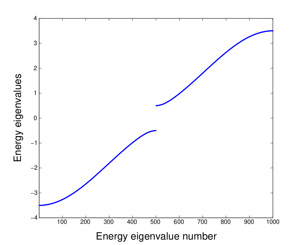
Numerically solving for the energy spectrum for a lattice model with a finite number of sites and parameters $\Delta_{0}$ and $\Delta_{1}$, we find that the energy dispersion is strikingly different in the two cases, $|\Delta_{0}|>|\Delta_{1}|$ and $|\Delta_{0}|<|\Delta_{1}|$. We find that for $|\Delta_{1}|<|\Delta_{0}|$, there are no states with energies lying within the superconducting gap. But for $|\Delta_{1}|>|\Delta_{0}|$, we find two states with zero energy which lie at the opposite ends of the system. This is shown in Fig. 1 for a $500$-site system with $\mu=0$, $\Delta_{0}=-2$, and $\Delta_{1}=2.5$ and $1.5$ (all in units of $\gamma$) in figures (a) and (b) respectively. The $x$-axis of the figures go from 1 to 1000 since each site $n$ of the lattice has two variables $c_{n}$ and $d_{n}$; hence there are 1000 states and 1000 energy levels. The energy eigenvalue number on the $x$-axis labels the energies in increasing order. (We have chosen a large enough number of sites so that if there are end modes, the hybridization between them is completely negligible and their energies will therefore be at zero energy exactly).

Figure 2: IPRs for a 500-site system with $\mu=0$, $\Delta_{0}=-2$, and (a) $\Delta_{1}=2.5$ and (b) $\Delta_{1}=1.5$. All energies are in units of $\gamma$. In figure (a) where $|\Delta_{1}|>|\Delta_{0}|$, we see that two of the states have a much higher IPR (about $0.14$) than all the other states (which are bulk states); the high IPR states correspond to the end modes. In figure (b) where $|\Delta_{1}|<|\Delta_{0}|$, all states have approximately the same IPR (about $0.0015$), and they are all bulk states. (The two kinks visible in the figure have no physical significance).

To distinguish between localized and extended states, we calculate the inverse participation ratio (IPR) calculated for all the eigenstates of the Hamiltonian. For the $j$-eigenstate $\psi_{j}$, let $\psi_{j,n}$ denote its $n$-th component, where $n$ goes from 1 to $2N$ (here $N$ is the number of lattice sites, and the factor of 2 arises as each site has two variables, $c_{n}$ and $d_{n}$). The IPR for $\psi_{j}$ is then defined as

$$I_{j}~=~\sum_{n}~|\psi_{j,n}|^{4}.$$ (10)

An extended state will generally have a value of the IPR which decreases as the system size increases, whereas a localized state will have a finite IPR whose value does not change with the system size. Hence a plot of the IPR $I_{j}$ versus $j$ for a large system size enables us to find the localized states easily. This is shown in Fig. 2 where the parameter values have been taken to be the same as in Fig. 1.

The system is said to be in a topologically non-trivial (trivial phase) if there are end modes (no end modes) respectively. The two phases can be distinguished from each other by a bulk topological invariant called the winding number. Since the Hamiltonian in Eq. (5) has a form given by $H(k)=a(k)\tau^{z}+b(k)\tau^{x}$, where $a(k)=\gamma\sin k-\mu$ and $b(k)=\Delta_{0}+\Delta_{1}\cos k$, we can consider a curve formed by points given by $(a(k),b(k))$. This forms a closed curve in two dimensions as $k$ goes from $0$ to $2\pi$. The winding number of this curve around the origin is defined as

$$W~=~\frac{1}{2\pi}\int_{0}^{2\pi}dk~~\dfrac{a~\partial b/\partial k~-~b~\partial a/\partial k}{a^{2}~+~b^{2}}.$$ (11)

This can be evaluated numerically for various values of $\Delta_{0}$ and $\Delta_{1}$. We find numerically that for $|\Delta_{1}|<|\Delta_{0}|$, the winding number $W=0$ and we are in a topologically trivial phase. For $|\Delta_{1}|>|\Delta_{0}|$, $W=\pm 1$ and we are in a topologically non-trivial phase.

It is instructive to look at the Fourier transforms of the wave functions of the end modes. Given the wave function $(c_{n},d_{n})$ of an end mode, we calculate the Fourier transforms $({\tilde{c}}_{k},{\tilde{d}}_{k})$, and plot $|{\tilde{c}}_{k}|^{2}+|{\tilde{d}}_{k}|^{2}$ versus $k$. This is shown in Fig. 3 for a 500-site system with $\Delta_{0}=-0.26$ and $\Delta_{1}=0.3$ in units of $\gamma$; we have taken $\mu=0$ in Fig. 3 (a) and $\mu=0.3$ in Fig. 3 (b). The locations and widths of the peaks in the two figures can be understood as follows. Since the end mode has zero energy, Eq. (6) implies that the momentum $k$ should satisfy

$$(\gamma\sin k~-~\mu)^{2}~+~(\Delta_{0}~+~\Delta_{1}\cos k)^{2}~=~0.$$ (12)

For $\mu,~\Delta_{0},~\Delta_{1}\ll\gamma$, the solution of Eq. (12) is given by

$$k~\simeq~\frac{\mu~\pm~i~|\Delta_{0}~+~\Delta_{1}|}{\gamma}.$$ (13)

For the mode at the left end, the wave function $c_{n},~d_{n}\sim e^{ikn}$ should have the imaginary part of $k$ positive so that the wave function goes to zero as $n\to+\infty$. Hence we must take $k=(\mu+i|\Delta_{0}+\Delta_{1}|)/\gamma$, implying that the wave function goes as $e^{in(\mu+i|\Delta_{0}+\Delta_{1}|)/\gamma}$. The Fourier transform of this has a peak at $k=\mu/\gamma$ and a width equal to $2|\Delta_{0}+\Delta_{1}|/\gamma$. This agrees with the locations and widths of the peaks that we see in Fig. 3.

Figure 3: Absolute value squared of the Fourier transform, $|{\tilde{c}}_{k}|^{2}+|{\tilde{d}}_{k}|^{2}$, of the wave function of the mode at the left end of a 500-site system with $\Delta_{0}=-0.26$ and $\Delta_{1}=0.3$. All energies are in units of $\gamma$. In (a), $\mu=0$ and the Fourier transform has a peak at $k=0$. In (b), $\mu=0.3$ and the Fourier transform has a peak at $k=0.3$. In both cases, the peak width at half maximum is about $0.08$.

We would like to emphasize here that our model has only one zero energy mode at each end of a long system, in contrast to conventional TRITOPS which have a Kramers pair of zero energy modes at each end [57, 58, 59, 60, 61, 62, 63, 64, 65]. While we have shown this numerically above, we can also show this analytically for the special case corresponding to $\mu=\Delta_{0}=0$. We will look for zero energy modes localized near the left end of a semi-infinite system where the sites go as $n=0,1,2,\cdots$. For zero energy, the left hand sides of Eqs. (3) vanish; we then obtain the recursion relation

$$\left(\begin{array}[]{c}c_{n+2}\\ d_{n+2}\end{array}\right)~=~\frac{1}{\gamma^{2}~-~\Delta_{1}^{2}}~\left(\begin{array}[]{cc}\gamma^{2}~+~\Delta_{1}^{2}&-i2\gamma\Delta_{1}\\ i2\gamma\Delta_{1}&\gamma^{2}~+~\Delta_{1}^{2}\end{array}\right)~\left(\begin{array}[]{c}c_{n}\\ d_{n}\end{array}\right)$$ (14)

for $n\geq 1$, and

$$-i\gamma c_{1}~+~\Delta_{1}d_{1} = 0,$$

$$i\gamma d_{1}~+~\Delta_{1}c_{1} = 0.$$ (15)

If $\Delta_{1}\neq\pm\gamma$, Eq. (15) gives $c_{1}=d_{1}=0$; Eq. (14) then implies that $c_{n}=d_{n}=0$ for all odd values of $n$. Next, the eigenvalues of the matrix appearing on the right hand side of Eq. (14) are given by $(\gamma+\Delta_{1})/(\gamma-\Delta_{1})$ and $(\gamma-\Delta_{1})/(\gamma+\Delta_{1})$. If $\gamma$ and $\Delta_{1}$ have the same sign the first eigenvalue is larger than 1 while the second eigenvalue is smaller than 1. To get a normalizable state, we must choose $(c_{n},d_{n})^{T}$ to be the eigenstate corresponding to the second eigenvalue. This implies the unique solution

$$\left(\begin{array}[]{c}c_{n}\\ d_{n}\end{array}\right)~=~\left(\frac{\gamma~-~\Delta_{1}}{\gamma~+~\Delta_{1}}\right)^{n/2}~\left(\begin{array}[]{c}1\\ -i\end{array}\right),$$ (16)

up to an overall normalization, where $n=0,2,4,\cdots$. We have confirmed that this matches the numerical results for the zero energy mode at the left end of the system. (We note that our analytical solution for the end mode of a semi-infinite system has some similarities with the solutions discussed earlier for the end modes of a finite-sized Kitaev chain and some of its generalizations [49, 50, 51, 52, 53]).

Before ending this section, we would like to comment on the fermion doubling problem which generally plagues lattice models with a massless Dirac Hamiltonian [86] and which does not appear in continuum models such as the one discussed in the next section. For instance, if we set $\mu=\Delta_{0}=\Delta_{1}=0$ in Eq. (5), the energy given by $\pm\gamma\sin k$ vanishes at both $k=0$ (which has a smooth continuum limit) and $k=\pi$ (which does not have a smooth continuum limit). We may therefore worry that the end modes that we have found numerically may be artefacts of the lattice model and more specifically of fermion doubling. However, we find numerically that this is not so. If we choose $\Delta_{0}$ and $\Delta_{1}$ to have opposite signs and close to each other in magnitude, and $\mu=0$, we see from Eq. (6) that the superconducting gap vanishes at $k=0$ and not $k=\pi$. We then find that the absolute value squared of the Fourier transform, $|{\tilde{c}}_{k}|^{2}+|{\tilde{d}}_{k}|^{2}$, of the wave function of the end modes is much larger around $k=0$ than around $k=\pi$ (see Fig. 3). Thus the doubled modes appearing near $k=\pi$ do not contribute significantly to the end modes. Further, we will see in Sec. III that the continuum model also has end modes, confirming that the modes near $k=0$ of the lattice model have a smooth continuum limit.

II.3 Symmetries of the model

We would now like to discuss some of the symmetries of our model. It is convenient to separately discuss symmetries of the Schrödinger equations in Eqs. (3) which act on wave functions and symmetries of the Hamiltonian in Eq. (1) which act on second-quantized operators.

We find that Eqs. (3) have the following two symmetries.

(i) Combination of $t\to-t$ and particle-hole symmetry: Eqs. (3) remain the same if we change $t\to-t$, $c_{n}\to d_{n}$ and $d_{n}\to-c_{n}$. (Note that we do not do complex conjugation). Hence, if there is a solution with wave function $(c_{n},d_{n})$ and energy $E$, there will also be a solution with wave function $(d_{n},-c_{n})$ and the opposite energy $-E$ (since $e^{-iEt/\hbar}\to e^{iEt/\hbar}$ under $t\to-t$). The combination of these two symmetries, called chiral symmetry [87], explains why we have a winding number as a topological invariant.

(ii) Combination of complex conjugation, $t\to-t$ and parity: Eqs. (3) remain the same if we complex conjugate them, change $t\to-t$, and invert $n\to-n$. This implies that if there is a solution with wave function $(c_{n},d_{n})$ and energy $E$, there will also be a solution with wave function $(c^{*}_{-n},d^{*}_{-n})$ and the same energy $E$ (since $e^{-iEt/\hbar}$ remains the same under complex conjugation and $t\to-t$).

These symmetries imply that if we take a finite-sized system and there is only one mode localized at, say, the left end, then its energy must be equal to zero (due to symmetry (i)), and there must also be a zero energy mode localized at the right end (due to symmetry (ii)). These agree with the numerical results presented in Sec. II.2.

Symmetry (i) also implies that if there is a zero energy mode at one end of a system, the expectation value of the charge in that mode, given by

$$Q~=~-e~\sum_{n}~(|c_{n}|^{2}-|d_{n}|^{2})$$ (17)

(where $-e$ is the electron charge), must be invariant under $c_{n}\to d_{n}$ and $d_{n}\to-c_{n}$, and must therefore be equal to zero.

We now discuss the symmetries of the Hamiltonian in Eq. (1). We find that there are two antiunitary symmetries.

(i) Time-reversal, i.e., spin-reversal and complex conjugation: Eq. (1) remains the same if we transform $c_{n\uparrow}\to c_{n\downarrow}$, $c_{n\downarrow}\to-c_{n\uparrow}$, and do complex conjugation. We note that the square of this transformation is equal to $-1$. The existence of this symmetry implies that the symmetry class of this system is DIII [87, 88, 89].

(ii) Combination of complex conjugation and parity: Eq. (1) remains the same if we transform $c_{n\uparrow}\to c_{-n\uparrow}$, $c_{n\downarrow}\to c_{-n\downarrow}$, and do complex conjugation. The square of this transformation is $+1$.

The symmetries discussed above can be broken in a variety of ways. A simple example is given by the case where the on-site superconducting pairing $\Delta_{0}$ is complex, so that the corresponding terms in Eq. (1) are given by $\Delta_{0}c_{n\uparrow}^{\dagger}c_{n\downarrow}^{\dagger}+\Delta^{*}_{0}c_{n\downarrow}c_{n\uparrow})$. We then find that both the symmetries given above are broken, although the combination of the two is still a symmetry (i.e., complex conjugate Eqs. (3) and change $c_{n}\to d^{*}_{-n}$ and $d_{n}\to-c^{*}_{-n}$), implying that if there is a mode at the left end with energy $E$, there will be a mode at the right end with energy $-E$. Numerically, we indeed find that if $\Delta_{0}$ is complex, the modes at the right and left ends generally have energies $E$ and $-E$ respectively, where $E\neq 0$. Further, Eq. (5) has an additional term given by ${\rm Im}(\Delta_{0})\tau^{y}$. Hence the Hamiltonian now has a combination of three Pauli matrices, i.e., Hamiltonian $H(k)=a(k)\tau^{z}+b(k)\tau^{x}+e(k)\tau^{y}$. As a function of $k$, $(a(k),b(k),e(k))$ defines a closed curve in three dimensions, instead of two dimensions. Hence it is no longer possible to define a winding number.

We can analytically find the energies of the end modes when $\Delta_{0}$ is complex as follows. We first take $\Delta_{0}$ to be real. We then know that Eqs. (3), which we can re-write as

$$-~\frac{i\gamma}{2}~(c_{n+1}~-~c_{n-1})~-~\mu~c_{n}$$

$$+~\Delta_{0}~d_{n}~+~\frac{\Delta_{1}}{2}~(d_{n+1}~+~d_{n-1})~=~Ec_{n},$$

$$\frac{i\gamma}{2}~(d_{n+1}~-~d_{n-1})~+~\mu~d_{n}$$

$$+~\Delta_{0}~c_{n}~+~\frac{\Delta_{1}}{2}~(c_{n+1}~+~c_{n-1})~=~Ed_{n},$$ (18)

has solutions at the ends with $E=0$. Further, we will see in Sec. III that if $\gamma>0$, the mode at the left end has $d_{n}=-ic_{n}$ while the mode at the right end has $d_{n}=ic_{n}$. This implies that for $E=0$, the two equations in (18) reduce to the equations

$$-~\frac{i\gamma}{2}~(c_{n+1}~-~c_{n-1})~-~\mu~c_{n}$$

$$\mp~i~\Delta_{0}~c_{n}~\mp~i~\frac{\Delta_{1}}{2}~(c_{n+1}~+~c_{n-1})~=~0,$$

$$\frac{i\gamma}{2}~(d_{n+1}~-~d_{n-1})~+~\mu~d_{n}$$

$$\pm~i~\Delta_{0}~d_{n}~\pm~i~\frac{\Delta_{1}}{2}~(c_{n+1}~+~c_{n-1})~=~0,$$ (19)

where the upper (lower) signs in both the equations hold for the left (right) end modes respectively. Now, suppose that $\Delta_{0}$ is complex; let us denote it by ${\tilde{\Delta}}_{0}$ to distinguish it from the real $\Delta_{0}$ in Eq. (19). Since the modes at the left (right) ends satisfy $d_{n}=\mp ic_{n}$ respectively, we obtain the equations

$$-~\frac{i\gamma}{2}~(c_{n+1}~-~c_{n-1})~-~\mu~c_{n}$$

$$\mp~i~{\tilde{\Delta}}_{0}~c_{n}~\mp~i~\frac{\Delta_{1}}{2}~(c_{n+1}~+~c_{n-1})~=~Ec_{n}$$

$$\frac{i\gamma}{2}~(d_{n+1}~-~d_{n-1})~+~\mu~d_{n}$$

$$\pm~i~{\tilde{\Delta}}^{*}_{0}~d_{n}~\pm~i~\frac{\Delta_{1}}{2}~(c_{n+1}~+~c_{n-1})~=~Ed_{n}.$$ (20)

We now observe that Eqs. (20) can be mapped to Eqs. (19) if we replace ${\rm Re}({\tilde{\Delta}}_{0})\to\Delta_{0}$ and $E\to\pm{\rm Im}({\tilde{\Delta}}_{0})$, where the $\pm$ hold for the left (right) end modes respectively. We thus conclude that when the on-site pairing $\Delta_{0}$ becomes complex, the wave functions $(c_{n},d_{n})$ of the end modes do not change (if we do not change the value of ${\rm Re}(\Delta_{0}$)), but their energies change from zero to $\pm{\rm Im}(\Delta_{0})$ at the left (right) ends respectively. Interestingly, the fact that the wave functions of the end modes do not change when $\Delta_{0}$ becomes complex implies that the expectation values of the charge (defined in Eq. (17)) remain equal to zero even though their energies become non-zero.

Figures 4 (a) and (b) show the effect of symmetry breaking on the end mode energies of a $500$-site system with $\mu=0$ and $\Delta_{1}=0.3$. In Fig. 4 (a), $\Delta_{0}=-0.26$ is real and each end has a zero energy mode. In Fig. 4 (b), $\Delta_{0}=-0.26e^{i\pi/50}$ is complex, and the end modes have energies $-0.0163$ (left end) and $0.0163$ (right end). We note that these values agree with $\pm{\rm Im}(\Delta_{0})$ respectively. (All energies are in units of $\gamma$).

Figure 4: Enlarged view of energy eigenvalues close to zero for a 500-site system with $\mu=0$, and $\Delta_{1}=0.3$. In (a), $\Delta_{0}=-0.26$ is real and each end has a zero energy mode. The superconducting gap is $0.081$. In (b), $\Delta_{0}=-0.26e^{i\pi/50}$ is complex, and the left (right) end has a mode with energy $-0.0163$ ($+0.0163$) respectively. The superconducting gap is $0.088$. All energies are in units of $\gamma$.

III Continuum model

We now consider a continuum model for a system with spin-orbit coupled Dirac Hamiltonian and an $s$-wave superconducting pairing which is a complex number. The continuum Hamiltonian is given by

$$H_{c} = \int dx~[-~i\gamma~(c^{\dagger}\partial_{x}c~-~d^{\dagger}\partial_{x}d)$$ (21)

$$~~~~~~~~~~+\Delta~e^{i\phi}~c^{\dagger}d~+~\Delta~e^{-i\phi}~d^{\dagger}c],$$

where $\gamma$ denotes the velocity. (We have assumed $\mu=0$ for simplicity). Note that the unlike the lattice model which has two different pairing parameters $\Delta_{0}$ and $\Delta_{1}$, a continuum model can only have one parameter $\Delta$. We saw in Sec. II that if $\Delta_{0}$ and $\Delta_{1}$ have opposite signs and are close to each other in magnitude, the long-distance properties of the lattice model are dominated by modes with momenta close to $k=0$. The form of the Hamiltonian in Eq. (5) then implies that the pairing $\Delta$ in the continuum model is related to the pairings $\Delta_{0},~\Delta_{1}$ in the lattice model as

$$\Delta~=~\Delta_{0}~+~\Delta_{1}.$$ (22)

Assuming the form in Eq. (4), Eq. (21) leads to the equation

$$\begin{pmatrix}-i\gamma\partial_{x}&\Delta e^{i\phi}\\ \Delta e^{-i\phi}&i\gamma\partial_{x}\end{pmatrix}\begin{pmatrix}\alpha\\ \beta\end{pmatrix}~=~E\begin{pmatrix}\alpha\\ \beta\end{pmatrix}.$$ (23)

This gives the energy spectrum

$$E~=~\pm\sqrt{\Delta^{2}+\gamma^{2}k^{2}}.$$ (24)

This has a gap from $-\Delta$ to $+\Delta$. In the rest of this section, we will set $\phi=0$ and $\Delta>0$. This can be done without loss of generality since we can absorb the phase $e^{i\phi}$ in $d$ in Eq. (21).

Figure 5: Schematic picture of a semi-infinite system terminated on the left at $x=0$. The $s$-wave pairing $\Delta e^{i\phi}$ is indicated.

This system has the same symmetries as discussed in Sec. II.3. Namely, the equations of motion remain invariant under under (i) $t\to-t$, $c(x)\to d(x)$, and $d(x)\to-c(x)$), and (ii) $t\to-t$, $c(x)\to c^{*}(-x)$, and $d(x)\to d^{*}(-x)$).

To study a localized mode which can appear at one end of the system, we now consider a semi-infinite system which is terminated at the left end, at $x=0$. The system goes from $x=0$ to $\infty$ as indicated in Fig. 5. To obtain a localized state whose energy lies within the superconducting gap, $-\Delta<E<\Delta$, we require a wave function which decays as $x$ increases. Hence the wave number $k$ appearing in Eq. (24) must have the form $k=(i/|\gamma|)\sqrt{\Delta^{2}-E^{2}}$.

Next, we impose the condition that the probability current $J$ must be zero at $x=0$. We can derive an expression for $J$ by defining the probability density $\rho=c^{\dagger}c+d^{\dagger}d$ and demanding that the equations of motion must lead to the equation of continuity, $\partial_{t}\rho+\partial_{x}J=0$. This gives $J=\gamma(c^{\dagger}c-d^{\dagger}d)$. We must therefore have $c^{\dagger}c-d^{\dagger}d=0$ at $x=0$. The general solution to this is $d=e^{i\theta}c$, where $\theta$ can be an arbitrary real parameter. However, the symmetry (i) mentioned above implies that we must have $e^{i\theta}=\pm i$, i.e., $\theta=\pm\pi/2$. Substituting this in the equations of motion, we obtain

$$\dfrac{E~-~i~{\rm sgn}(\gamma)\sqrt{\Delta^{2}-E^{2}}}{\Delta}~=~e^{i\theta},$$ (25)

where $\theta$ is $-\pi/2$ if $\gamma>0$ and $\pi/2$ if $\gamma<0$, and ${\rm sgn}(\gamma)$ denotes the sign of $\gamma$. In either case, we have $E=0$.

Similarly, for a system terminated at the right end, with $x$ decreasing as we go away from the end and into the system, we find that we must choose $k=-(i/|\gamma|)\sqrt{\Delta^{2}-E^{2}}$. We now find that the allowed values of $\theta$ are $\pi/2$ if $\gamma>0$ and $-\pi/2$ if $\gamma<0$.

These conditions on $\theta$ give the relation between the two components of the wave function as $\beta=\mp i\alpha$ at the left (right) ends respectively, if $\gamma>0$. We find numerically that the end modes of the lattice model indeed have $E=0$ and their wave functions satisfy the relations given above. We note here that the phase relation between the two components holds for all values of $x$, not just at the two ends. Namely, the mode localized at the left (right) end has $\beta(x)=\mp i\alpha(x)$ for all $x$.

IV General model with both Dirac and Schrödinger terms

In this section we will consider a more general model in which the Hamiltonian is a combination of a spin-orbit coupled Dirac Hamiltonian, a Schrödinger Hamiltonian, and an $s$-wave superconducting pairing. The motivation for this study is as follows. We know that in the presence of $s$-wave superconducting pairing, a purely Schrödinger Hamiltonian without a spin-orbit coupling term has no zero energy end modes, while a purely Dirac Hamiltonian with a spin-orbit coupled form does have such modes. We therefore want to know how a transition between the two phases occurs when going from one limit to the other.

We will take the total continuum Hamiltonian to be

$$H_{c} = \int dx~[-~i\gamma~(c^{\dagger}\partial_{x}c~-~d^{\dagger}\partial_{x}d)$$ (26)

$$~~~~~~~~~~-~\frac{\epsilon\hbar^{2}}{2m}~(c^{\dagger}\partial_{x}^{2}c~-~d^{\dagger}\partial_{x}^{2}d)$$

$$~~~~~~~~~~-~\epsilon\mu~(c^{\dagger}c~-~d^{\dagger}d)$$

$$~~~~~~~~~~+~\Delta~c^{\dagger}d~+~\Delta~d^{\dagger}c],$$

where we have chosen the pairing $\Delta$ to be real. In Eq. (26), $\epsilon$ is a tuning parameter: for $\epsilon=0$, we recover the Dirac Hamiltonian studied earlier, while for $\epsilon=1$, we obtain a Schrödinger Hamiltonian along with a spin-orbit interaction with strength $\gamma$. (In momentum space, the non-superconducting part of the Hamiltonian in Eq. (26) is given, in terms of spin-up and spin-down fields $c$ and $d^{\dagger}$, as $\epsilon(\hbar^{2}k^{2}/(2m)-\mu)I+\gamma k\sigma^{z}$, where $I$ is the identity matrix).

Given the probability density $\rho=c^{\dagger}c+d^{\dagger}d$, the equations of motion and continuity imply that the current is

$$J = -~\frac{i\epsilon\hbar}{2m}~(c^{\dagger}\partial_{x}c~-~\partial_{x}c^{\dagger}c~-~d^{\dagger}\partial_{x}d~+~\partial_{x}d^{\dagger}d)$$ (27)

$$+~\gamma~(c^{\dagger}c~-~d^{\dagger}d).$$

For a semi-infinite system which goes from $x=0$ to $\infty$, we have to impose the condition $J=0$ at $x=0$ for all the modes. For $\epsilon=0$, we saw above that the general condition which gives zero current at $x=0$ is $c=e^{i\theta}d$. However, for $\epsilon=1$ and $\gamma=0$, we know that the usual condition at a hard wall is given by $c=0$ and $d=0$. This is not the most general possible condition which gives zero current for the Schrödinger Hamiltonian [90, 91]. However we always require two conditions unlike the case of the Dirac Hamiltonian where we need only one condition ($c=e^{i\theta}d$). When both $\epsilon$ and $\gamma$ are non-zero, it is therefore not obvious what condition should be imposed on $c$, $d$ and their derivatives at $x=0$.

We therefore turn to a lattice version of this model. The Hamiltonian for such a model is obtained by adding the following

$$\delta H_{l} = -\frac{g}{2}~\sum_{n}~[c_{n\uparrow}^{\dagger}c_{n+1\uparrow}~+~c_{n\downarrow}^{\dagger}c_{n+1\downarrow}~+~{\rm H.c.}]$$ (28)

to the Hamiltonian given in Eq. (1). The eigenvalue equation therefore changes from Eq. (5) to

$$[(\gamma\sin k-g\cos k-\mu)\tau^{z}+(\Delta_{0}+\Delta_{1}\cos k)\tau^{x}]\begin{pmatrix}\alpha\\ \beta\end{pmatrix}$$ (29)

$$= E\begin{pmatrix}\alpha\\ \beta\end{pmatrix},$$

which gives

$$E=\pm\sqrt{(\gamma\sin k-g\cos k-\mu)^{2}+(\Delta_{0}+\Delta_{1}\cos k)^{2}}.$$ (30)

We now consider what happens if the parameters $\gamma,~\mu,~\Delta_{0}$ and $\Delta_{1}$ are held fixed and $g$ is varied. Eq. (30) implies that the energy gap will be zero if there is a value of $k$ where $\gamma\sin k-g\cos k-\mu=0$ (which requires $\sqrt{\gamma^{2}+g^{2}}>|\mu|$) and $\Delta_{0}+\Delta_{1}\cos k=0$. The second condition requires $|\Delta_{0}/\Delta_{1}|\leq 1$. Using this in the first condition then implies that the energy gap will be zero at $g=g_{\pm}$ where

$$g_{\pm}~=~\frac{\mu\Delta_{1}}{\Delta_{0}}~\pm~\gamma~\sqrt{\left(\frac{\Delta_{1}}{\Delta_{0}}\right)^{2}~-~1}.$$ (31)

Numerically, we find that if $(\Delta_{0}/\Delta_{1})^{2}<1$ and $g$ lies between the values $g_{\pm}$ given in Eq. (31), the system lies in a topologically non-trivial phase and there is a zero energy mode at each end of a finite-sized system. But if $g$ lies outside this range, there are no end modes. We find that this also agrees with a winding number calculation. Defining $a(k)=\gamma\sin k-g\cos k-\mu$ and $b(k)=\Delta_{0}+\Delta_{1}\cos k$, we find that the winding number defined in Eq. (11) is $\pm 1$ if $g_{-}<g<g_{+}$ (consistent with a topologically non-trivial phase) and is zero outside this range (giving a topologically trivial phase). The model therefore hosts two topological transitions between these phases at $g=g_{\pm}$.

Finally, we note that the equations of motion for the model defined above have the same two symmetries that we discussed in Sec. II.3. This explains why the end modes have zero energy.

V Josephson effects for two superconducting systems with different phases

V.1 Andreev bound states at a Josephson junction

Figure 6: Schematic picture of a junction between two $s$-wave superconductors with pairings $\Delta e^{i\phi_{1}}$ ($\Delta e^{i\phi_{2}}$) for $x<0$ ($>0$) respectively. The junction at $x=0$ has a $\delta$-function barrier with strength $\lambda$.

In this section, we will study the ABS and the Josephson current between two superconducting systems in which the $s$-wave pairings have different phases. We first consider a continuum model. We will take the magnitudes of the two pairings (and hence the superconducting gaps) to be equal, and their phases to be $\phi_{1}$ and $\phi_{2}$. Further, the two systems will be taken to be separated by a $\delta$-function potential barrier with strength $\lambda$ located at $x=0$. A schematic picture of the system is shown in Fig. 6. The continuum Hamiltonians on the two sides of $x=0$ are given by

$$H_{c1} = \int_{-\infty}^{0}dx~[-~i\gamma~(c^{\dagger}\partial_{x}c~-~d^{\dagger}\partial_{x}d)$$

$$~~~~~~~~~~~~~~+~\Delta~e^{i\phi_{1}}~c^{\dagger}d~+~\Delta~e^{-i\phi_{1}}~d^{\dagger}c],$$

$$H_{c2} = \int_{0}^{\infty}dx~[-~i\gamma~(c^{\dagger}\partial_{x}c~-~d^{\dagger}\partial_{x}d)$$ (32)

$$~~~~~~~~~~~~~~+~\Delta~e^{i\phi_{2}}~c^{\dagger}d~+~\Delta~e^{-i\phi_{2}}~d^{\dagger}c],$$

where $H_{c1}$ ($H_{c2}$) is the Hamiltonian on the left (right) of the $\delta$-function barrier respectively.

The equations of motion following from Eqs. (32), along with a time-dependence of $c$ and $d$ of the form $e^{-iEt/\hbar}$, take the form

$$-i\gamma~\partial_{x}c~+~\Delta e^{i\phi_{i}}~d~=~E~c,$$

$$i\gamma~\partial_{x}d~+~\Delta e^{-i\phi_{i}}~c~=~E~d,$$ (33)

where $\phi_{i}=\phi_{1}~(\phi_{2})$ for $x<0~(>0)$ respectively. Complex conjugating the above equations implies that there is a symmetry under

$$\phi_{i}\to\pi-\phi_{i}~~~{\rm and}~~~E\to-E.$$ (34)

Eqs. (33) imply the energy dispersion $E=\pm\sqrt{\Delta^{2}+\gamma^{2}k^{2}}$, and the second-quantized operators have the form

$$c_{k}(x) = e^{i(kx-Et)}~f_{k},$$

$$d_{k}(x) = \dfrac{E-\gamma k}{\Delta}~e^{i(kx-Et)-i\phi}~f_{k}.$$ (35)

To find the ABS, the wave number $k$ has to be chosen in such a way that the wave functions decay away from the $\delta$-potential, towards $x\to\pm\infty$ on the two sides. From this condition we obtain

$$k_{1} = -~\frac{i}{\gamma}~\sqrt{\Delta^{2}-E^{2}}~~~{\rm on~the~left},$$

$${\rm and}~~~k_{2} = \frac{i}{\gamma}~\sqrt{\Delta^{2}-E^{2}}~~~{\rm on~the~right}.$$ (36)

The boundary condition at $x=0$ takes the form

$$c(x=0+) = e^{-i\lambda/\gamma}~c(x=0-),$$

$$d(x=0+) = e^{-i\lambda/\gamma}~d(x=0-).$$ (37)

(We recall that for a Hamiltonian of the Dirac form, a $\delta$-function potential leads to a discontinuity in the wave function. This is unlike a Hamiltonian of the Schrödinger form where a $\delta$-function gives a discontinuity in the first derivative of the wave function). Since the phase jumps across $x=0$ are equal for $c$ and $d$, we will see that the $\delta$-potential has no effect on expressions for quantities like the energy spectrum and hence the Josephson current. Using the boundary condition in Eq. (37), we can find the value of the ABS energy. We find that the energy depends only on the phase difference $\phi_{2}-\phi_{1}$ and has the form

$$E~=~-~\Delta~{\rm sgn}(\gamma)~\cos\left(\dfrac{[\phi_{2}-\phi_{1}]}{2}\right),$$ (38)

where we define the function $[\phi_{2}-\phi_{1}]=\phi_{2}-\phi_{1}$ modulo $2\pi$. Namely, it is a periodic function of $\phi_{2}-\phi_{1}$ with period $2\pi$, and it lies in the range $0<[\phi_{2}-\phi_{1}]<2\pi$. (If $\phi_{2}-\phi_{1}$ is exactly equal to a multiple of $2\pi$, there is, strictly speaking, no ABS since such the energy of such a state must satisfy $-\Delta<E<\Delta$). According to Eq. (38), when $\phi_{2}-\phi_{1}$ approaches a multiple of $2\pi$, the energy of the ABS approaches $\pm\Delta$. Eqs. (36) then implies that the decay length of the ABS diverges as $\gamma/\sqrt{\Delta^{2}-E^{2}}$; hence the ABS becomes indistinguishable from the bulk states. Figure 7 shows the ABS energy $E$ in units of $\Delta$ (red solid curve) as a function of $\phi_{2}-\phi_{1}$, taking $\gamma>0$. We see that as $\phi_{2}-\phi_{1}$ crosses a multiple of $2\pi$, an ABS disappears after touching the top of the superconducting gap and a different ABS appears from the bottom of the gap.

We thus find the peculiar result that there is only one ABS for each value of $\phi_{2}-\phi_{1}$. One way of understanding why there is only one ABS instead of two is to note that in our model, there are only right-moving spin-up and left-moving spin-down electrons. The ABS is formed by a right-moving spin-up electron which moves from the left superconductor towards the junction and gets reflected as a left-moving spin-down hole; alternatively, a left-moving spin-down electron moves from the right superconductor towards the junction and gets reflected as a right-moving spin-up hole.

The appearance of a single ABS with the energy given in Eq. (38) is consistent with a particle-hole transformation in which we transform $c\to d$ and $d\to-c$. This transforms our system to a different one in which the phases $\phi_{1}$ and $\phi_{2}$ have the opposite signs and whose Hamiltonian also has the opposite sign. Hence all the energy levels (including the ABS) of the second system should be negative of the energy levels of the original system. Indeed we see from Eq. (38) that the sign of the ABS energy flips when $\phi_{i}\to-\phi_{i}$.

We also note that if our sample has a large but finite width, the states at the opposite edges would have opposite signs of the velocity $\gamma$ in Eq. (32); this is a property of Dirac electrons at the boundaries of a topological insulator. If both edges are in proximity to the same superconductors so that $\phi_{1}$ and $\phi_{2}$ have the same values at the two edges, the energies of the ABSs at the two edges will have opposite signs. We can see this from Eq. (38) where the expression for the energy has a factor of ${\rm sgn}(\gamma)$.

Figure 7: Plots of the Andreev bound state energy (red solid curve) in units of $\Delta$ and the Josephson current in units of $e\Delta/\hbar$ (blue dashed curve) versus $\phi_{2}-\phi_{1}$, taking $\phi_{1}=0$ and $\gamma>0$.

Next, we consider the AC Josephson effect. We will consider zero temperature for simplicity and take $\gamma>0$. If a small constant voltage bias $V_{0}$ is applied to the superconductor lying in the region $x>0$, the pairing phase there will change slowly in time as

$$\phi_{2}~=~\frac{2eV_{0}t}{\hbar}.$$ (39)

Then the Josephson current will be given by

$$I_{J} = \dfrac{2e}{\hbar}\dfrac{\partial E}{\partial(\phi_{2}-\phi_{1})}$$ (40)

$$= \frac{e\Delta}{\hbar}~|\sin\left(\dfrac{\phi_{2}-\phi_{1}}{2}\right)|,$$

where $\phi_{2}$ changes in time according to Eq. (39), and $I_{J}$ is a function of $\phi_{2}-\phi_{1}$ with a periodicity of $2\pi$ as discussed after Eq. (38). Figure 7 shows the Josephson current $I_{J}$ (blue dashed curve) in units of $e\Delta/\hbar$ as a function of $\phi_{2}-\phi_{1}$. Note that $I_{J}$ has no discontinuity at any value of $\phi_{2}-\phi_{1}$.

Interestingly, we see that $I_{J}$ is always non-negative, and therefore its average value (which is also equal to its time-averaged value since $\phi_{2}$ varies linearly with time) is positive. This is unlike the AC Josephson effect found in most systems where the average value of $I_{J}$ is zero; hence $I_{J}$ does not have a DC part in those systems. Note also that at certain times, $\phi_{2}-\phi_{1}$ will cross odd-integer multiples of $\pi$; then the ABS bound state will cross zero energy giving rise to a fermion-parity switch [92].

We also note as $\phi_{2}-\phi_{1}$ changes in time from zero to $2\pi$, a quasiparticle appears from the bottom of the superconducting gap and moves up in energy to reach the top of the gap. Since this quasiparticle carries spin-up (we recall that both $c^{\dagger}=c_{\uparrow}^{\dagger}$ and $d^{\dagger}=c_{\downarrow}$ increase the spin component $S^{z}$ by $\hbar/2$), we have a process of spin pumping from the left superconductor to the right superconductor; an amount of $S^{z}=\hbar/2$ is pumped in a time period $2\pi/\omega_{J}$, where $\omega_{J}=2eV_{0}/\hbar$ is the Josephson frequency.

Figure 8: Probability $|c_{n}|^{2}+|d_{n}|^{2}$ versus $n$ of the Andreev bound state wave function which appears in the middle of a 500-site system with pairing $\phi_{1}=0$ in the left half and $\phi_{2}=\pi/2$ in the right half of the system. We have taken $\mu=0$, $\Delta_{0}=-0.26$, $\Delta_{1}=0.3$. The energy of the Andreev bound state is $-0.028$, and the superconducting gap is $0.084$. All energies are in units of $\gamma$.

We have confirmed the dispersion given in Eq. (38) by doing numerical calculations for a lattice model. We consider a $500$-site system with pairing $\phi_{1}=0$ in the left half and $\phi_{2}=\pi/2$ in the right half of the system. We take $\Delta_{0}=-0.26$ and $\Delta_{1}=0.3$, so that the pairing of the corresponding continuum model (given by the modes near $k=0$ of the lattice model) is given by $\Delta=\Delta_{0}+\Delta_{1}=0.04$. We find that there is only one ABS which lies in the middle of the system; its energy is $-0.028$ which agrees well with the value of $-\Delta\cos((\phi_{2}-\phi_{1}/2)/2)$ given by Eq. (38). (All energies are in units of $\gamma$). Figure 8 shows the wave function of this ABS. We have checked numerically that the Fourier transform of the wave function is sharply peaked around $k=0$ (similar to Fig. 3 (a)), showing once again that the lattice modes near $k=\pi$ do not contribute to the ABS. Interestingly, we find that the expectation value of the charge (Eq. (17)) is zero in the ABS for any value of its energy.

V.2 Shapiro plateaus

In this section, we will study the phenomenon of Shapiro plateaus in a resistively and capacitively shunted Josephson junction. In this system, a resistance $R$ and a capacitance $C$ are placed in parallel with a Josephson junction [81, 82, 83, 84, 85].

Denoting $\phi=\phi_{2}-\phi_{1}$ as the phase difference across the Josephson junction, the current across the junction is given by Eq. (40). The voltage bias across the Josephson junction is given by

$$V~=~\frac{\hbar}{2e}~\frac{d\phi}{dt}.$$ (41)

The current across the resistance and capacitor are then given by $V/R$ and $CdV/dt$ respectively. The total current is given by the sum of these three currents. We now impose the condition that the total current has a constant term $I$ and a term which oscillates with time as $A\sin(\omega t)$. We thus have the equation

$$C\frac{dV}{dt}~+~\frac{V}{R}~+~\frac{e\Delta}{\hbar}~|\sin(\frac{\phi}{2})|~=~I~+~A\sin(\omega t).$$ (42)

Using Eq. (41) and introducing the dimensionless time variable $\tau=\omega t$, we can rewrite Eq. (42) as

$$\alpha_{1}~\frac{d^{2}\phi}{d\tau^{2}}~+~\alpha_{2}~\frac{d\phi}{d\tau}~+~\frac{2\Delta}{\hbar\omega}~|\sin(\frac{\phi}{2})| = \frac{2}{e\omega}~[I~+~A\sin\tau],$$

$${\rm where}~~~~\alpha_{1}~=~\frac{\hbar\omega C}{e^{2}}~~~~{\rm and}~~~~\alpha_{2} = \frac{\hbar}{e^{2}R}.$$ (43)

We will solve Eq. (43) numerically from $\tau=0$ to $\tau=\tau_{0}$ where $\tau_{0}$ is a large number (say, $200\pi$ corresponding to 100 driving cycles of the current) and find the average value of the voltage bias

$$\langle~V~\rangle = \frac{\hbar\omega}{2e}~\langle~\frac{d\phi}{d\tau}~\rangle$$ (44)

$$= \frac{\hbar\omega}{2e}~\frac{\phi(\tau_{0})~-~\phi(0)}{\tau_{0}}.$$

For large values of $\tau_{0}$, we find numerically that $\langle V\rangle$ given by Eq. (44) does not depend on the initial values of $\phi$ and $d\phi/d\tau$ at $\tau=0$.

We will now provide a qualitative understanding of why Shapiro plateaus should appear in a plot of $\langle V\rangle$ versus $I$. Let us first set $\Delta=0$. Eq. (43) then has the solution

$$\phi = \chi_{1}\tau~+~\chi_{2}\sin(\tau+\chi_{3})~+~\phi_{0},$$

$${\rm where}~~~\chi_{1} = \frac{2I}{e\omega\alpha_{2}},$$

$$\chi_{2} = -~\frac{2A}{e\omega\sqrt{\alpha_{1}^{2}~+~\alpha_{2}^{2}}},$$

$$\chi_{3} = \tan^{-1}\left(\frac{\chi_{2}}{\chi_{1}}\right),$$ (45)

where $\phi_{0}$ is a constant of integration. The first term in Eq. (45) along with Eq. (41) means that the voltage bias will have an average value given by

$$\langle V\rangle~=~\frac{\hbar\omega\chi_{1}}{2e}.$$ (46)

We now substitute Eq. (45) in the third term of the right hand side of Eq. (43). (This procedure can be justified perturbatively if $\Delta$ is a small parameter). At this point it is useful to do a Fourier transform of the function $|\sin(\pi/2)|$. The Fourier components are given by

$$F_{m} = \int_{0}^{2\pi}\frac{d\phi}{2\pi}~e^{-im\phi}~|\sin(\phi/2)|$$ (47)

$$= \frac{2}{\pi}~\frac{1}{1~-~4m^{2}}.$$

Note that $F_{m}=F_{-m}$ is real. The third term in Eq. (43) then takes the form

$$\frac{2\Delta}{\hbar\omega}\sum_{m=-\infty}^{\infty}F_{m}~e^{im(\chi_{1}\tau~+~\chi_{2}\sin(\tau+\chi_{3})~+~\phi_{0})}$$

$$= \frac{2\Delta}{\hbar\omega}\sum_{m=-\infty}^{\infty}F_{m}e^{im(\chi_{1}\tau~+~\phi_{0})}~\sum_{n=-\infty}^{\infty}J_{n}(m\chi_{2})~e^{in(\tau+\chi_{3})},$$

where we have used Eq. (45) to substitute for $\phi$ in the first line, and the Bessel functions in the second line satisfy $J_{-n}(z)=J_{n}(-z)=(-1)^{n}J_{n}(z)$. [93]. We now see that the expression in Eq. () will have a DC part which does not vary with $\tau$ whenever

$$\chi_{1}~=~-~\frac{n}{m},$$ (49)

where $m,~n$ are integers, and we assume that $m\neq 0$. The corresponding DC part in Eq. () is equivalent to shifting the constant $I$ on the right hand side of Eq. (43) by

$$\frac{e\Delta}{\hbar}~[F_{m}J_{n}(m\chi_{2})e^{im\phi_{0}}~+~F_{-m}J_{-n}(-m\chi_{2})e^{-im\phi_{0}}]$$ (50)

$$= \frac{2e\Delta}{\hbar}~F_{m}J_{n}(m\chi_{2})\cos(m\phi_{0}).$$

Since Eq. (50) can have a range of values depending on $\phi_{0}$ (since $\cos(m\phi_{0})$ can vary from $-1$ to $+1$), we see that $I$ can have a range of values given by

$$\frac{4e\Delta}{\hbar}~F_{m}J_{n}(m\chi_{2}).$$ (51)

For all these values of $I$, we see from Eqs. (46) and (49) that $\langle V\rangle$ will have a fixed value given by

$$\langle V\rangle~=~-~\frac{\hbar\omega}{2e}~\frac{n}{m}.$$ (52)

This explains why there should be a plateau in $\langle V\rangle$ for a range of values of $I$, whenever Eq. (52) is satisfied. The width of the Shapiro plateau will be proportional to $(4e\Delta/\hbar)F_{m}J_{n}(m\chi_{2})$. Hence the plateau widths go to zero rapidly as either $m$ or $n$ increases since $F_{m}$ goes to zero as $1/m^{2}$ as $m\to\infty$ and $J_{n}(z)$ goes to zero as $(ez/2n)^{n}$ as $n\to\infty$ keeping $z$ fixed.

We would like to mention here that the series of plateaus corresponding to $m=1,2,3,\cdots$ in Eq. (52) has no analog in standard Josephson junctions where $I_{J}\propto\sin\phi$, and the Fourier transform of $I_{J}$ is non-zero only for $m=\pm 1$. We note that the appearance of such plateaus for rational fractional values of $\omega_{J}/\omega$ has been noted in a different context in Ref. 94.

We now present our numerical results. For our calculations, we choose the parameters in Eq. (43) as follows: $\hbar\omega=100~\mu$eV which implies $\omega\simeq 152$ GHz, $\alpha_{1}=1$ implying $C\simeq 1.6\times 10^{-3}$ pF, $\alpha_{2}=1$ implying $R\simeq 4.11$ k$\Omega$, and $\Delta=100~\mu$eV. (This value of the induced superconducting gap $\Delta$ is appropriate for a NbSe₂/Bi₂Se₃ superconductor-topological insulator heterostructure [95]). Eq. (43) then takes the form

$$\frac{d^{2}\phi}{d\tau^{2}}~+~\frac{d\phi}{d\tau}~+~2~|\sin(\frac{\phi}{2})|~=~\frac{2}{e\omega}~[I~+~A\sin\tau].$$ (53)

In Fig. 9, we show a plot of $\langle V\rangle$ versus $I$ for $A=2$. We note that $I$ and $A$ are given in units of $e\omega=24$ nA, and $\langle V\rangle$ is in units of $\hbar\omega/e=100~\mu$V. Fig. 9 shows several plateaus in $\langle V\rangle$. The most prominent plateaus occur for $\langle V\rangle$ equal to multiples of $\hbar\omega/(2e)$ corresponding to the denominator $m$ in Eq. (52) being equal to 1. But some small plateaus are also visible at multiples of $\hbar\omega/(4e)$, $\hbar\omega/(3e)$, and $\hbar\omega/(6e)$ corresponding to $m=2$ and $n$ odd, $m=3$ and $n$ even, and $m=3$ and $n$ odd in Eq. (52).

Fig. 9 shows that the plateau at $\langle V\rangle=0$ occurs at non-zero values of $I$. This happens because the time-averaged value of the left hand side of Eq. (53) is given by the average of $2|\sin(\phi/2)|$ over one cycle of $\phi$ from 0 to $2\pi$ which is equal to $4/\pi$. This means that the time-averaged value of the right hand side of Eq. (53) is also $4/\pi$. This explains why the midpoint of the plateau at $\langle V\rangle=0$ lies at about $I/(e\omega)=2/\pi\simeq 0.637$ in Fig. 9. (This is in contrast to other Josephson junctions where the current is proportional to $\sin\phi$ or $\sin(\phi/2)$ whose average over one cycle is equal to zero).

Finally, the comment made earlier that a change of $\phi$ by $2\pi$ pumps an amount of spin angular momentum equal to $\hbar/2$ across the junction means that the rate of transfer of angular momentum is given by $\hbar/2$ times $d\phi/dt/(2\pi)$. Eq. (41) then implies that plateaus in $\langle V\rangle$ are equivalent to plateaus in the average rate of transfer of angular momentum; the two are related as

$$\frac{\hbar}{2}~\frac{\langle{d\phi/dt}\rangle}{2\pi}~=~\frac{e\langle V\rangle}{2\pi}.$$ (54)

Figure 9: Plot of $\langle V\rangle$ versus $I$. We have chosen $\alpha_{1}=\alpha_{2}=1$, $\Delta=100~\mu$eV, $A=2$, and $\hbar\omega=100~\mu$eV. $I$ and $A$ are in units of $e\omega=24$ nA, and $V$ is in units of $\hbar\omega/e=100~\mu$V. We see that $\langle V\rangle$ has several plateaus of different widths at fractional multiples of $\hbar\omega/(2e)$. The midpoint of the plateau at $\langle V\rangle=0$ lies at about $I=2/\pi$. See text for details.

VI Discussion

In this paper we have presented a minimal model of a TRITOPS using the chirality of Dirac electrons on a thin, effectively one-dimensional, strip of a topological insulator surface. Our model is time-reversal invariant but it possesses half the number of modes of the more well-studied time-reversal-invariant topological superconductors due to the chirality of the underlying Dirac electrons. This property leads to several unconventional features which we have charted out.

We first consider a lattice model of a spin-orbit coupled massless Dirac electron in one dimension with $s$-wave superconducting pairing. We analytically find the bulk energy spectrum, and use a topological invariant called the winding number to identify the regimes of parameter values where the system is in topologically trivial and non-trivial phases. In the topologically non-trivial phase, a finite-sized system has a single zero energy Majorana mode at each end; we find that this requires the $s$-wave pairing to have an extended form with the magnitude of the nearest-neighbor pairing being larger than that of the on-site pairing. For a particular choice of parameters, we present an analytical expression for the wave function of an end mode. Although a lattice model of massless Dirac electrons may suffer from a fermion doubling problem, we find that this can be avoided in our model if we take the on-site and nearest-neighbor $s$-wave pairings to have opposite signs and close to each other in magnitude. Then the wave functions of both the bulk states lying near the gap and the end modes have momentum components close to $k=0$ rather than $k=\pi$. The modes near $k=0$ have a smooth continuum limit.

We study the symmetries of the lattice model if both the $s$-wave pairings are real. These symmetries imply that if there is only one mode at each end, it must have zero energy and the expectation value of the charge in such mode will be zero; this is in agreement with our numerical results. We then consider the effect of making the on-site pairing complex. We find that this shifts the energies of the end modes away from zero, but the expectation value of the charge remains zero.

We then consider a continuum version of the model with a completely local $s$-wave pairing. If the pairing is real, this model always turns out to have zero energy modes at the ends of a long system. The ratio of the phases of the spin-up electron and spin-down hole wave functions is either $+i$ or $-i$ for the end modes, and this is found to be in agreement with the lattice results.

Next, we study a lattice system whose Hamiltonian is a combination of a Schrödinger Hamiltonian and a spin-orbit coupled Dirac Hamiltonian, along with a local $s$-wave pairing. We find that this system is necessarily topologically trivial if the Dirac part is absent and can be topologically non-trivial if the Schrödinger part is absent. We analytically find the parameter values at which a topological transition occurs from one phase to the other. It is worth noting that an external magnetic field is not required to generate end modes in any of our models, either on the lattice or in the continuum.

We then study a Josephson junction of two continuum systems which have different phases of the $s$-wave pairing, called $\phi_{1}$ and $\phi_{2}$. In contrast to the earlier models of TRITOPS, we find that there is a single ABS which is localized near the junction; its energy depends on the phase difference $\Delta\phi=\phi_{2}-\phi_{1}$ with a period $2\pi$, but it does not depend on the strength of a potential barrier which may be present at the junction (this is related to the Dirac nature of the electrons which imposes matching conditions on the electron and hole wave functions but not on their derivatives). As $\Delta\phi$ varies from 0 to $2\pi$, the ABS energy goes smoothly from the bottom of the superconducting gap to the top. We then study some Josephson effects at zero temperature. First, we examine the AC Josephson effect where a time-independent voltage bias $V_{0}$ is applied across the junction. Since this makes $\Delta\phi$ change linearly in time, an ABS which initially has negative energy (and is therefore filled) moves smoothly to positive energy values; this process repeats periodically in time. We therefore find that the Josephson current, which is given by the derivative of the ABS energy with respect to $\Delta\phi$, varies periodically in time with a frequency given by $\omega_{J}=2eV_{0}/\hbar$. The Josephson current turns out be a continuous function of $\Delta\phi$. However, its sign does not change with $\Delta\phi$ which implies that the current has a non-zero DC component; this is in contrast to the AC Josephson effect studied earlier in other systems. Second, we consider a resistively and capacitively shunted Josephson junction and study what happens when the voltage bias has both a constant term $V_{0}$ as a term $V_{1}\cos(\omega t)$ which oscillates sinusoidally with an amplitude $V_{1}$ and a frequency $\omega$. We find that the Josephson current can then exhibit Shapiro plateaus whenever $\omega_{J}$ is a rational multiple of $\omega$, i.e., $\omega_{J}=(n/m)\omega$, where $m,~n$ are integers. However the plateau widths rapidly go to zero as $m$ or $n$ increases; in particular, if $eV_{1}/(\hbar\omega)$ is small, only the plateaus with $n=1$ and different values of $m$ would be observable. The presence of such Shapiro plateaus when $\omega_{J}/\omega$ is a rational fraction distinguishes these Josephson junctions from their standard $s$- or $p$-wave counterparts.

We discuss a few platforms on which our model may be experimentally realized. A bulk insulating three-dimensional topological insulator where one of the surfaces has strong finite-size quantization, allows the formation of one-dimensional Dirac-like bands that propagate along the surface. Inducing superconducting by proximity effect on one such surface with a conventional $s$-wave superconductor may realize our model and allow the formation of Majorana bound states at the sample edges as we discuss here. One-dimensional Dirac-like states may also be trapped on one-dimensional crystalline defects that naturally occur on van der Waals bonded three-dimensional topological insulators such as Bi₂Se₃ [66, 67]. Edges between two facets of a bulk crystal of such a material may also host such one-dimensional modes. The proximity of such a state to an $s$-wave superconductor will realize our model. In the context of two-dimensional topological insulators, our model may be realized by inducing superconductivity using proximity effect on one of the edges of the sample, leaving the other edge non-proximitized. In a Josephson junction configuration, the existence of one Andreev bound state, rather than a pair of Andreev bound states as conventionally observed, is a striking manifestation of our model. Various experimental methods including tunneling spectroscopy  [96, 97], Josephson spectroscopy [98, 99] and circuit quantum electrodynamics schemes [100, 101] may be used to detect the presence of a “single” Andreev bound state. We further predict that the Josephson supercurrent in such a geometry is always positive, which can be detected by DC electrical transport. We envisage that such experiments are already possible on various two-dimensional and three-dimensional topological insulator materials that are currently known. Such platforms provide an alternate route towards realization of Majorana bound states that could potentially display large topological gaps, and exist at zero magnetic field and at higher temperatures than currently possible.

Acknowledgments

We thank the referees for useful suggestions. A.B. would like to thank MHRD, India for financial support and P. S. Anil Kumar for experimental work that inspired some of the ideas. D.S. thanks DST, India for Project No. SR/S2/JCB-44/2010 for financial support. K.S. thanks DST for support through INT/RUS/RFBR/P-314.

References

- [2] A. Kitaev, Physics-Uspekhi 44, 131 (2001).
- [3] C. Nayak, S. H. Simon, A. Stern, M. Freedman, and S. Das Sarma, Rev. Mod. Phys. 80, 1083 (2008).
- [4] J. Alicea, Y. Oreg, G. Refael, F. von Oppen, and M. P. A. Fisher, Nature Phys. 7, 412 (2011).
- [5] R. M. Lutchyn, J. D. Sau, and S. Das Sarma, Phys. Rev. Lett. 105, 077001 (2010).
- [6] Y. Oreg, G. Refael, and F. von Oppen, Phys. Rev. Lett. 105, 177002 (2010).
- [7] A. C. Potter and P. A. Lee, Phys. Rev. Lett. 105, 227003 (2010).
- [8] V. Shivamoggi, G. Refael, and J. E. Moore. Phys. Rev. B 82, 041405(R) (2010).
- [9] I. C. Fulga, F. Hassler, A. R. Akhmerov, and C. W. J. Beenakker, Phys. Rev. B 83, 155429 (2011).
- [10] S. B. Chung, H.-J. Zhang, X.-L. Qi, and S.-C. Zhang, Phys. Rev. B 84, 060510(R) (2011).
- [11] E. Sela, A. Altland, and A. Rosch, Phys. Rev. B 84, 085114 (2011).
- [12] T. D. Stanescu, R. M. Lutchyn, and S. Das Sarma, Phys. Rev. B 84, 144522 (2011).
- [13] R. M. Lutchyn and M. P. A. Fisher, Phys. Rev. B 84, 214528 (2011).
- [14] S. Gangadharaiah, B. Braunecker, P. Simon, and D. Loss, Phys. Rev. Lett. 107, 036801 (2011).
- [15] A. R. Akhmerov, J. P. Dahlhaus, F. Hassler, M. Wimmer, and C. W. J. Beenakker, Phys. Rev. Lett. 106, 057001 (2011).
- [16] Y. Niu, S. B. Chung, C.-H. Hsu, I. Mandal, S. Raghu, and S. Chakravarty, Phys. Rev. B 85, 035110 (2012).
- [17] P. W. Brouwer, M. Duckheim, A. Romito, and F. von Oppen, Phys. Rev. B 84, 144526 (2011).
- [18] P. W. Brouwer, M. Duckheim, A. Romito, and F. von Oppen, Phys. Rev. Lett. 107, 196804 (2011).
- [19] M. Gibertini, F. Taddei, M. Polini, and R. Fazio, Phys. Rev. B 85, 144525 (2012).
- [20] R. Egger and K. Flensberg, Phys. Rev. B 85, 235462 (2012).
- [21] M. Tezuka and N. Kawakami, Phys. Rev. B 85, 140508(R) (2012).
- [22] D. Sticlet, C. Bena, and P. Simon, Phys. Rev. Lett. 108, 096802 (2012); D. Chevallier, D. Sticlet, P. Simon, and C. Bena, Phys. Rev. B 85, 235307 (2012).
- [23] L. Fidkowski, J. Alicea, N. H. Lindner, R. M. Lutchyn, and M. P. A. Fisher, Phys. Rev. B 85, 245121 (2012).
- [24] J. Klinovaja and D. Loss, Phys. Rev. B 86, 085408 (2012).
- [25] J. S. Lim, L. Serra, R. López, and R. Aguado, Phys. Rev. B 86, 121103(R) (2012).
- [26] A. M. Cook, M. M. Vazifeh, and M. Franz, Phys. Rev. B 86, 155431 (2012).
- [27] F. L. Pedrocchi, S. Chesi, S. Gangadharaiah, and D. Loss, Phys. Rev. B 86, 205412 (2012).
- [28] A. M. Lobos, R. M. Lutchyn, and S. Das Sarma, Phys. Rev. Lett. 109, 146403 (2012).
- [29] S. Tewari and J. D. Sau, Phys. Rev. Lett. 109, 150408 (2012).
- [30] P. San-Jose, E. Prada, and R. Aguado, Phys. Rev. Lett. 108, 257001 (2012); E. Prada, P. San-Jose, and R. Aguado, Phys. Rev. B 86, 180503(R) (2012).
- [31] J. Alicea, Rep. Prog. Phys. 75, 076501 (2012).
- [32] J. D. Sau and S. Das Sarma, Nature Communications 3, 964 (2012).
- [33] J. D. Sau, C. H. Lin, H.-Y. Hui, and S. Das Sarma, Phys. Rev. Lett. 108, 067001 (2012).
- [34] L.-J. Lang and S. Chen, Phys. Rev. B 86, 205135 (2012).
- [35] C. W. J. Beenakker, Annu. Rev. Condens. Matter Phys. 4, 113 (2013).
- [36] T. D. Stanescu and S. Tewari, J. Phys. Condens. Matter 25, 233201 (2013).
- [37] Y. Asano and Y. Tanaka, Phys. Rev. B 87, 104513 (2013).
- [38] W. DeGottardi, D. Sen, and S. Vishveshwara, Phys. Rev. Lett. 110, 146404 (2013).
- [39] W. DeGottardi, M. Thakurathi, S. Vishveshwara, and D. Sen, Phys. Rev. B 88, 165111 (2013).
- [40] X. Cai, L.-J. Lang, S. Chen, and Y. Wang, Phys. Rev. Lett. 110, 176403 (2013).
- [41] I. Adagideli, M. Wimmer, and A. Teker, Phys. Rev. B 89, 144506 (2014).
- [42] S. Sarkar, Scientific Reports 6, 30569 (2016).
- [43] V. Chua, K. Laubscher, J. Klinovaja, and D. Loss, Phys. Rev. B 102, 155416 (2020).
- [44] V. Mourik, K. Zuo, S. M. Frolov, S. R. Plissard, E. P. A. M. Bakkers, and L. P. Kouwenhoven, Science 336, 1003 (2012).
- [45] M. T. Deng, C. L. Yu, G. Y. Huang, M. Larsson, P. Caroff, and H. Q. Xu, Nano Lett. 12, 6414 (2012).
- [46] L. P. Rokhinson, X. Liu, and J. K. Furdyna, Nature Phys. 8, 795 (2012).
- [47] A. Das, Y. Ronen, Y. Most, Y. Oreg, M. Heiblum, and H. Shtrikman, Nature Phys. 8, 887 (2012).
- [48] A. D. K. Finck, D. J. Van Harlingen, P. K. Mohseni, K. Jung, and X. Li, Phys. Rev. Lett. 110, 126406 (2013).
- [49] A. A. Zvyagin, Phys. Rev. Lett. 110, 217207 (2013) and Low Temp. Phys. 41, 625 (2015).
- [50] H.-c. Kao, Phys. Rev. B 90, 245435 (2014).
- [51] S. Hegde, V. Shivamoggi, S. Vishveshwara, and D. Sen, New J. Phys. 17, 053036 (2015).
- [52] N. Leumer, M. Marganska, B. Muralidharan, and M. Grifoni, J. Phys. Condens. Matter 32, 445502 (2020).
- [53] K. Kawabata, R. Kobayashi, N. Wu, and H. Katsura, Phys. Rev. B 95, 195140 (2017).
- [54] M. Z. Hasan and C. L. Kane, Rev. Mod. Phys. 82, 3045 (2010).
- [55] X.-L. Qi and S.-C. Zhang, Rev. Mod. Phys. 83, 1057 (2011).
- [56] S. Ray, S. Mukerjee, and N. Shah, arXiv:2003.08299.
- [57] F. Zhang, C. L. Kane, and E. J. Mele, Phys. Rev. Lett. 111, 056402 (2013).
- [58] F. Zhang, C. L. Kane, and E. J. Mele, Phys. Rev. Lett. 111, 056403 (2013).
- [59] E. Gaidamauskas, J. Paaske, and K. Flensberg, Phys. Rev. Lett. 112, 126402 (2014).
- [60] A. Camjayi, L. Arrachea, A. Aligia, and F. von Oppen, Phys. Rev. Lett. 119, 046801 (2017).
- [61] A. A. Aligia and L. Arrachea, Phys Rev. B 98, 174507 (2018).
- [62] L. Arrachea, A. Camjayi, A. A. Aligia, and L. Gruńeiro, Phys Rev. B 99, 085431 (2019).
- [63] A. A. Aligia and A. Camjayi, Phys Rev. B 100, 115413 (2019).
- [64] A. Haim and Y. Oreg, Phys. Rep. 825, 1 (2019).
- [65] S. V. Aksenov, A. O. Zlotnikov, and M. S. Shustin, Phys. Rev. B 101, 125431 (2020).
- [66] Z. Alpichshev, J. G. Analytis, J.-H. Chu, I. R. Fisher, and A. Kapitulnik, Phys. Rev. B 84, 041104(R) (2011).
- [67] A. Kandala, A. Richardella, D. Zhang, T. C. Flanagan, and N. Samarth, Nano Lett. 13, 2471 (2013).
- [68] M.-X. Wang, C. Liu, J.-P. Xu, F. Yang, L. Miao, M.-Y. Yao, C. L. Gao, C. Shen, X. Ma, X. Chen, Z.-A. Xu, Y. Liu, S.-C. Zhang, D. Qian, J.-F. Jia, and Q.-K. Xue, Science 336, 52 (2012).
- [69] S.-Y. Xu, N. Alidoust, I. Belopolski, A. Richardella, C. Liu, M. Neupane, G. Bian, S.-H. Huang, R. Sankar, C. Fang, B. Dellabetta, W. Dai, Q. Li, M. J. Gilbert, F. Chou, N. Samarth, and M. Z. Hasan, Nature Phys. 10, 943 (2014).
- [70] D. Flötotto, Y. Ota, Y. Bai, C. Zhang, K. Okazaki, A. Tsuzuki, T. Hashimoto, J. N. Eckstein, S. Shin, and T.-C. Chiang, Science Advances 4, 7214 (2018).
- [71] D. B. Szombati, S. Nadj-Perge, D. Car, S. R. Plissard, E. P. A. M. Bakkers, and L. P. Kouwenhoven, Nature Phys. 12, 568 (2016).
- [72] F. Pientka, A. Keselman, E. Berg, A. Yacoby, A. Stern, and B. I. Halperin, Phys. Rev. X 7, 021032 (2017).
- [73] A. Fornieri, A. M. Whiticar, F. Setiawan, E. P. Marín, A. C. C. Drachmann, A. Keselman, S. Gronin, C. Thomas, T. Wang, R. Kallaher, G. C. Gardner, E. Berg, M. J. Manfra, A. Stern, C. M. Marcus, and F. Nichele, Nature 569, 89 (2019).
- [74] H. Ren, F. Pientka, S. Hart, A. Pierce, M. Kosowsky, L. Lunczer, R. Schlereth, B. Scharf, E. M. Hankiewicz, L. W. Molenkamp, B. I. Halperin, and Amir Yacoby, Nature 569, 93 (2019).
- [75] A. Stern and E. Berg, Phys. Rev. Lett. 122, 107701 (2019).
- [76] S. Hart, H. Ren, T. Wagner, P. Leubner, M. Mühlbauer, C. Brüne, H. Buhmann, L. W. Molenkamp, and A. Yacoby, Nature Phys. 10, 638 (2014).
- [77] J. Wiedenmann, E. Bocquillon, R. S. Deacon, S. Hartinger, O. Herrmann, T. M. Klapwijk, L. Maier, C. Ames, C. Brüne, C. Gould, A. Oiwa, K. Ishibashi, S. Tarucha, H. Buhmann, and L. W. Molenkamp, Nature Comm. 7, 10303 (2016).
- [78] Y. Tanaka, T. Hirai, K. Kusakabe, and S. Kashiwaya, Phys. Rev. B 60, 6308 (1999).
- [79] C. D. Vaccarella, R. D. Duncan, and C. A. R. Sá de Melo, Physica C 391, 89 (2003).
- [80] H.-J. Kwon, K. Sengupta, and V. M. Yakovenko, Eur. Phys. J. B 37, 349 (2004).
- [81] J. B. Ketterson and S. N. Song, Superconductivity (Cambridge University Press, Cambridge, 1999).
- [82] Y. M. Shukrinov, S. Y. Medvedeva, A. E. Botha, M. R. Kolahchi, and A. Irie, Phys. Rev. B 88, 214515 (2013).
- [83] M. Maiti, K. V. Kulikov, K. Sengupta, and Y. M. Shukrinov, Phys. Rev. B 92, 224501 (2015).
- [84] E. Bocquillon, R. S. Deacon, J. Wiedenmann, P. Leubner, T. M. Klapwijk, C. Brüne, K. Ishibashi, H. Buhmann and L. W. Molenkamp, Nature Nanotech. 12, 137 (2017).
- [85] O. Deb, K. Sengupta, and D. Sen, Phys. Rev. B 97, 174518 (2018).
- [86] H. B. Nielsen and M. Ninomiya, Nucl. Phys. B 193, 173 (1981); H. B. Nielsen and M. Ninomiya, Phys. Lett. B 105, 219 (1981).
- [87] A. P. Schnyder, S. Ryu, A. Furusaki, and A. W. W. Ludwig, Phys. Rev. B 78, 195125 (2008).
- [88] J. C. Y. Teo and C. L. Kane, Phys. Rev. B 82, 115120 (2010).
- [89] L. Fidkowski and A. Kitaev, Phys. Rev. B 83, 075103 (2011).
- [90] M. Carreau, J. Phys. A 26, 427 (1993).
- [91] W. A. Harrison, Applied Quantum Mechanics (World Scientific, Singapore, 2000), pp. 119-120.
- [92] B. Tarasinski, D. Chevallier, J. A. Hutasoit, B. Baxevanis, and C. W. J. Beenakker, Phys. Rev. B 92, 144306 (2015).
- [93] M. Abramowitz and I. A. Stegun, Handbook of Mathematical Functions (Dover, New York, 1972).
- [94] R. Ghosh, M. Maiti, Y. M. Shukrinov, and K. Sengupta, Phys. Rev. B 96, 174517 (2017).
- [95] W. Dai, A. Richardella, R. Du, W. Zhao, X. Liu, C. X. Liu, S.-H. Huang, R. Sankar, F. Chou, N. Samarth, and Q. Li, Scientific Reports 7, 7631 (2017).
- [96] E. J. H. Lee, X. Jiang, R. Aguado, G. Katsaros, C. M. Lieber, and S. DeFranceschi, Phys. Rev. Lett. 109, 186802 (2012).
- [97] J. D. Pillet, C. H. L. Quay, P. Morfin, C. Bena, A. Levy Yeyati, and P. Joyez, Nature Phys. 6, 965 (2010).
- [98] L. Bretheau, C. O. Girit, H. Pothier, D. Esteve, and C. Urbina, Nature 499, 3125 (2013).
- [99] D. J. V. Woerkom, A. Proutski, B. V. Heck, D. Bouman, J. I. Vayrynen, L. I. Glazman, P. Krogstrup, J. Nygard, L. P. Kouwenhoven, and A. Geresdi, Nature Phys. 13, 8761 (2017).
- [100] M. Hays, G. de Lange, K. Serniak, D. J. van Woerkom, D. Bouman, P. Krogstrup, J. Nygard, A. Geresdi, and M. H. Devoret, Phys. Rev. Lett. 121, 047001 (2018).
- [101] L. Tosi, C. Metzger, M. F. Goffman, C. Urbina, H. Pothier, S. Park, A. Levy Yeyati, J. Nygard, and P. Krogstrup, Phys. Rev. X 9, 011010 (2019).