Neuro-Symbolic Visual Reasoning: Disentangling “Visual” from “Reasoning”

Abstract

Visual reasoning tasks such as visual question answering (VQA) require an interplay of visual perception with reasoning about the question semantics grounded in perception. However, recent advances in this area are still primarily driven by perception improvements (e.g. scene graph generation) rather than reasoning. Neuro-symbolic models such as Neural Module Networks bring the benefits of compositional reasoning to VQA, but they are still entangled with visual representation learning, and thus neural reasoning is hard to improve and assess on its own. To address this, we propose (1) a framework to isolate and evaluate the reasoning aspect of VQA separately from its perception, and (2) a novel top-down calibration technique that allows the model to answer reasoning questions even with imperfect perception. To this end, we introduce a differentiable first-order logic formalism for VQA that explicitly decouples question answering from visual perception. On the challenging GQA dataset, this framework is used to perform in-depth, disentangled comparisons between well-known VQA models leading to informative insights regarding the participating models as well as the task.

1 Introduction

Figure 1: The multi-step question answering process in the $\nabla$-FOL framework, based on differentiable first-order logic.

Visual reasoning (VR) is the ability of an autonomous system to construct a rich representation of a visual scene and perform multi-step inference over the scene’s constituents and their relationships. It stands among the key outstanding challenges in computer vision. Common tangible instantiations of VR include language-driven tasks such as Visual Question Answering (VQA) (Antol et al., 2015) and Visual Commonsense Reasoning (VCR) (Zellers et al., 2019). Recent advances in computer vision, representation learning, and natural language processing have enabled continued progress on VQA with a wide variety of modeling approaches (Hudson & Manning, 2019a; Andreas et al., 2016; Anderson et al., 2018; Hudson & Manning, 2018; Tan & Bansal, 2019).

A defining characteristic of VR is the interaction between a perception system (i.e. object detection and scene representation learning) and a reasoning system (i.e. question interpretation and inference grounded in the scene). However, this interaction is difficult to capture and assess accurately. For example, the definition of VQA has evolved over time to eliminate language biases that impeded its robustness as a VR metric. The early VQA datasets were biased to real-world language priors to the extent that many questions were answerable without looking at the image (Agrawal et al., 2018). Subsequent versions improved the balance but still mostly involved simple inference questions with little requirement for multi-step reasoning.

To facilitate progress in VR, Hudson & Manning (2019b) proposed GQA, a procedurally generated VQA dataset of multi-step inference questions. Although GQA targets compositional multi-step reasoning, the current GQA Challenge primarily evaluates visual perception rather than reasoning of a VQA model. As we show in Section 4, a neuro-symbolic VQA model that has access to ground-truth scene graphs achieves 96% accuracy on GQA. Moreover, language interpretation (i.e. semantic parsing) alone does not capture the complexity of VR due to the language in questions being procedurally generated. As a result, while GQA is well suited as an evaluation environment for VR (e.g. for multi-modal pretraining tasks (Tan & Bansal, 2019; Zhou et al., 2020)), a higher GQA accuracy does not necessarily imply a higher reasoning capability. In this work, we supplement GQA with a differentiable first-order logic framework $\nabla$-FOL that allows us to isolate and assess the reasoning capability of a VQA model separately from its perception.

The $\nabla$-FOL Framework: $\nabla$-FOL is a neuro-symbolic VR model. Neuro-symbolic models such as MAC (Hudson & Manning, 2018), Neural Module Networks (Andreas et al., 2016), and Neural State Machines (Hudson & Manning, 2019a) implement compositional multi-step inference by modeling each step as a differentiable operator from a functional specification of the question (i.e. a program) or its approximation. This facilitates systematicity, compositionality, and out-of-distribution generalization in VQA because accurate inference of a given question commonly requires accurate inference over its constituents and entailed questions (Vedantam et al., 2019). They, however, commonly operate over the latent feature representations of objects and their relations, produced by the underlying perception module. This entanglement not only limits interpretability of the learned neuro-symbolic inference blocks, but also limits the reasoning techniques applicable for VQA improvement.

In contrast to SOTA neuro-symbolic approaches, $\nabla$-FOL fully disentangles visual representation learning of a VQA model from its inference mechanism, while still being end-to-end trainable with backpropagation (see Figure 1). This enables identifying GQA questions solvable via perception vs. reasoning and evaluating their respective contributions.

VQA Reasoning Evaluation Score: To assess the reasoning capability of a VQA model, we define the VQA reasoning evaluation score as the extent to which the model can answer a question despite imperfect visual perception. If the input image is noisy or the perception system is imperfect, the learned object representations do not contain enough information to determine certain attributes of the objects. This potentially impedes question answering and may require non-trivial reasoning. For example, an object detection module that misclassifies wolves as huskies may impede answering the question “Is there a husky in the living room?” Similarly, the question “What is behind the broken wooden chair?” relies on the information capturing “broken”, “wooden”, and “chair” attributes in the representation of the corresponding object. Many VQA models answer such questions nonetheless (e.g. by disregarding weak attribute signals when a strong “chair” signal is present in a single object in the scene), which exemplifies the kind of visual reasoning we aim to assess in VQA. In contrast, the questions that can be answered using a pre-trained perception system and parameter-less logical inference do not require reasoning per se as their visual representations contain all the information necessary to answer the question.

Contributions: This work makes three contributions:

• We introduce differentiable first-order logic as a common formalism for compositional visual reasoning and use it as a foundation for the inference in $\nabla$-FOL.

• We use $\nabla$-FOL to define a disentangled evaluation methodology for VQA systems to assess the informativeness of perception as well as the power of reasoning separately. To this end, we introduce a VQA reasoning evaluation score, an augmentation of GQA evaluation that eliminates questions primarily resolved by perception. With it, we evaluate two representatives from two families of VQA models: MAC (Hudson & Manning, 2018) and LXMERT (Tan & Bansal, 2019).

• As a simple way of going beyond logical reasoning, we propose top-down calibration via the question context on the top of FOL reasoning and show that it improves the accuracy of $\nabla$-FOL on the visually hard questions.

2 Related Work and Background

Visual Question Answering: VQA has been used as a front-line task to research and advance VR capabilities. The first release of the VQA dataset (Antol et al., 2015) initiated annual competitions and a wide range of modeling techniques aimed at addressing visual perception, language understanding, reasoning, and their combination (Lu et al., 2019; Tan & Bansal, 2019; Hudson & Manning, 2018; Hudson & Manning, 2019a; Anderson et al., 2018; Li et al., 2019; Zhou et al., 2020). To reduce the annotation effort and control the problem complexity, CLEVR (Johnson et al., 2017) and GQA (Hudson & Manning, 2019b) tasks propose synthetic construction of resp. scenes and questions.

Capturing and measuring the extent of human ability in VR accurately is a significant challenge in task design as well as modeling. Datasets have to account for language and real-world biases, such as non-visual and false-premise questions (Ray et al., 2016). VQA models, when uncontrolled, are known to “solve” the task by e.g. exploiting language priors (Agrawal et al., 2016; Zhou et al., 2015). Different techniques have been proposed to control this phenomenon. Agrawal et al. (2018) adversarially separate the distributions of training and validation sets. Goyal et al. (2017) balance the VQA dataset by asking human subjects to identify distractors – visually similar images that yield different answers for the same questions. Recently, Selvaraju et al. (2020) augment the VQA dataset with human-annotated subquestions that measure a model’s reasoning consistency in answering complex questions. In this work, we propose another step to improve the accuracy of VQA reasoning assessment by capturing a “hard” subset of GQA questions where perception produces imperfect object representations.

Neuro-Symbolic Reasoning: $\nabla$-FOL is a neuro-symbolic reasoning model (Garcez et al., 2019). In neuro-symbolic reasoning, answer inference is defined as a chain of differentiable modules wherein each module implements an “operator” from a latent functional program representation of the question. The approach is applicable to a wide range tasks, including visual QA (Andreas et al., 2016; Vedantam et al., 2019; Hudson & Manning, 2018), reading comprehension of natural language (Chen et al., 2020), and querying knowledge bases, databases, or other structured sources of information (Saha et al., 2019; Neelakantan et al., 2015; Neelakantan et al., 2016; Liang et al., 2016). The operators can be learned, like in MAC (Hudson & Manning, 2018) or pre-defined, like in NMN (Andreas et al., 2016). In contrast to semantic parsing (Liang, 2016) or program synthesis (Gulwani et al., 2017; Parisotto et al., 2016), the model does not necessarily emit a symbolic program, although it can involve them as an intermediate step to construct the differentiable pipeline (like in $\nabla$-FOL). Neuro-symbolic reasoning is also similar to neural program induction (NPI) (Reed & De Freitas, 2015; Cai et al., 2017; Pierrot et al., 2019) but the latter requires strong supervision in the form of traces, and the learned “operators” are not always composable or interpretable.

The main benefit of neuro-symbolic models is their compositionality. Because the learnable parameters of individual operators are shared for all questions and subsegments of the differentiable pipeline correspond to constituents of each question instance, the intermediate representations produced by each module are likely composable with each other. This, in turn, facilitates interpretability, systematicity, and out-of-distribution generalization – commonly challenging desiderata of reasoning systems (Vedantam et al., 2019). In Section 6, we demonstrate them in $\nabla$-FOL over VQA.

Neuro-symbolic models can be partially or fully disentangled from the representation learning of their underlying ground-world modality (e.g. vision in the case of VQA). Partial entanglement is the most common, wherein the differentiable reasoning operates on featurizations of the scene objects rather than raw pixels but the featurizations are in the uninterpretable latent space. Neural State Machine (NSM) (Hudson & Manning, 2019a) and the eXplainable and eXplicit Neural Modules (XNM) (Shi et al., 2019) are prominent examples of such frameworks. As for full disentanglement, there are Neural-Symbolic Concept Learner (NS-CL) (Mao et al., 2019) and Neural-Symbolic VQA (NS-VQA) (Yi et al., 2018) which separate scene understanding, semantic parsing, and program execution with symbolic representations in between similar to $\nabla$-FOL. However, both NS-CL and NS-VQA as well as XNM are based on operators that are heuristic realization of the task-dependent domain specific language (DSL) of their target datasets. In contrast, we propose a task-independent, mathematical formalism that is probabilistically derived from the first-order logic independent of any specific DSL. This highlights two important differences between $\nabla$-FOL and NS-CL, NS-VQA, or XNM. First, compared to these frameworks, $\nabla$-FOL is more general-purpose: it can implement any DSL that is representable by FOL. Second, our proposed disentangled evaluation methodology in Section 4 requires the reasoning framework to be mathematically sound so that we can reliably draw conclusions based off it; this is the case for our FOL inference formalism. Furthermore, while NS-CL and NS-VQA have only been evaluated on CLEVR (with synthetic scenes and a limited vocabulary), $\nabla$-FOL is applied to real-life scenes in GQA.

Finally, we note that outside of VR, logic-based, differentiable neuro-symbolic formalisms have been widely used to represent knowledge in neural networks (Serafini & Garcez, 2016; Socher et al., 2013; Xu et al., 2018). A unifying framework for many of such formalisms is Differentiable Fuzzy Logics (DFL) (van Krieken et al., 2020) which models quantified FOL within the neural framework. Despite the similarity in formulation, the inference in DFL is generally of exponential complexity, whereas $\nabla$-FOL proposes a dynamic programming strategy to perform inference in polynomial time, effectively turning it into program-based reasoning of recent VQA frameworks. Furthermore, while these frameworks have been used to encode symbolic knowledge into the loss function, $\nabla$-FOL is used to specify a unique feed-forward architecture for each individual instance in the dataset; in that sense, $\nabla$-FOL is similar to recent neuro-symbolic frameworks proposed to tackle the SAT problem (Selsam et al., 2018; Amizadeh et al., 2018; Amizadeh et al., 2019).

3 Differentiable First-Order Logic for VR

We begin with the formalism of differentiable first-order logic (DFOL) for VR systems, which forms the foundation for the $\nabla$-FOL framework. DFOL is a formalism for inference over statements about an image and its constituents. It has two important properties: (a) it disentangles inference from perception, so that e.g. the operation "filter all the red objects in the scene" can be split into determining the “redness” of every object and attending to the ones deemed sufficiently red, and (b) it is end-to-end differentiable, which allows training the perception system from inference results. In Section 4, we show how DFOL enables us to measure reasoning capabilities of VQA models.

3.1 Visual Perception

Given an image $\mathcal{I}$, let $\mathcal{V}=\{\bm{v}_{1},\bm{v}_{2},...,\bm{v}_{N}\}$ be a set of feature vectors $\bm{v}_{i}\in\mathbb{R}^{d}$ representing a set of $N$ objects detected in $\mathcal{I}$. This detection can be done via different pre-trained models such as Faster-RCNN (Ren et al., 2015) for object detection or Neural Motifs (Zellers et al., 2018) or Graph-RCNN (Yang et al., 2018) for scene graph generation. As is common in VQA, we assume $\mathcal{V}$ as given, and refer to it as the scene visual featurization.

Furthermore, we introduce the notion of neural visual oracle $\mathcal{O}=\{\mathcal{M}_{f},\mathcal{M}_{r}\}$ where $\mathcal{M}_{f}$ and $\mathcal{M}_{r}$ are neural models parametrized by vectors $\bm{\theta}_{f}$ and $\bm{\theta}_{r}$, respectively. Conceptually, $\mathcal{M}_{f}(\bm{v}_{i},\pi\mid\mathcal{V})$ computes the likelihood of the natural language predicate $\pi$ holding for object $\bm{v}_{i}$ (e.g. $\mathcal{M}_{f}(\bm{v}_{i},"red"\mid\mathcal{V})$). Similarly, $\mathcal{M}_{r}(\bm{v}_{i},\bm{v}_{j},\pi\mid\mathcal{V})$ calculates the likelihood of $\pi$ holding for a pair of objects $\bm{v}_{i}$ and $\bm{v}_{j}$ (e.g. $\mathcal{M}_{r}(\bm{v}_{i},\bm{v}_{j},"holding"\mid\mathcal{V})$). $\mathcal{O}$ combined with the visual featurization forms the perception system of $\nabla$-FOL.

3.2 First-Order Logic over Scenes

Given $N$ objects in the scene, we denote by the upper-case letters $X,Y,Z,...$ categorical variables over the objects’ index set $I=\{1,...,N\}$. The values are denoted by subscripted lower-case letters – e.g. $X=x_{i}$ states that $X$ is set to refer to the $i$-th object in the scene. The $k$-arity predicate $\pi:I^{k}\mapsto\{\top,\bot\}$ defines a Boolean function on $k$ variables $X,Y,Z,...$ defined over $I$. In the context of visual scenes, we use unary predicates $\pi(\cdot)$ to describe object names and attributes (e.g. $\mathsf{Chair}(x_{i})$ and $\mathsf{Red}(y_{j})$), and binary predicates $\pi(\cdot,\cdot)$ to describe relations between pairs of objects (e.g. $\mathsf{On}(y_{j},x_{i})$). Given the definitions above, we naturally define quantified first-order logical (FOL) formulae $\mathcal{F}$, e.g.

$$\mathcal{F}(X,Y)=\exists X,\forall Y:\mathsf{Chair}(X)\land\mathsf{Left}(X,Y)$$ (1)

states that "There is a chair in the scene that is to the left of all other objects."

FOL is a more compact way to describe the visual scene than the popular scene graph (Yang et al., 2018) notation, which can be seen as a Propositional Logic description of the scene, also known as grounding the formula. More importantly, while scene graph is only used to describe the scene, FOL allows us to perform inference over it. For instance, the formula in Eq. (1) also encodes the binary question "Is there a chair in the scene to the left of all other objects?" In other words, a FOL formula encodes both a descriptive statement and a hypothetical question about the scene. This is the key intuition behind $\nabla$-FOL and the common formalism behind its methodology.

3.3 Inference

Given a NL (binary) question $\mathcal{Q}$ and a corresponding FOL formula $\mathcal{F_{Q}}$, the answer $a_{\mathcal{Q}}$ is the result of evaluating $\mathcal{F_{Q}}$. We reformulate this probabilistically as

$$\Pr(a_{\mathcal{Q}}=\text{``yes''}\mid\mathcal{V})=\Pr(\mathcal{F_{Q}}\Leftrightarrow\top\mid\mathcal{V})\triangleq\alpha(\mathcal{F_{Q}}).$$ (2)

The naïve approach to calculate the probability in Eq. 2 requires evaluating every instantiation of $\mathcal{F_{Q}}$, which are of exponential number. Instead, we propose a dynamic programming strategy based on the intermediate notion of attention which casts inference as a multi-hop execution of a functional program in polynomial time.

Assume $\mathcal{F_{Q}}$ is minimal and contains only the operators $\land$ and $\neg$ (which are functionally complete). We begin by defining the concept of attention which in $\nabla$-FOL naturally arises by instantiating a variable in the formula to an object:

Definition 3.1.

Given a FOL formula $\mathcal{F}$ over the variables $X,Y,Z,...$, the attention on the object $x_{i}$ w.r.t. $\mathcal{F}$ is:

$$\alpha(\mathcal{F}\mid x_{i}) \triangleq\Pr(\mathcal{F}_{X=x_{i}}\Leftrightarrow\top\mid\mathcal{V})$$ (3)

$$\qquad\text{ where }\mathcal{F}_{X=x_{i}} \triangleq\mathcal{F}(x_{i},Y,Z,...),\forall i\in[1..N]$$ (4)

Similarly, one can compute the joint attention $\alpha(\mathcal{F}\mid x_{i},y_{j},...)$ by fixing more than one variable to certain objects. For example, given the formula in Eq. 1, $\alpha(\mathcal{F}\mid x_{i})$ represents the probability that "The $i$-th object in the scene is a chair that is to the left of all other objects." and $\alpha(\mathcal{F}\mid y_{j})$ represents the probability that "The $j$-th object in the scene is to the right of a chair.".

Next, we define the attention vector on variable $X$ w.r.t. formula $\mathcal{F}$ as $\bm{\alpha}(\mathcal{F}\mid X)=[\alpha(\mathcal{F}\mid x_{i})]_{i=1}^{N}$. In similar way, we define the attention matrix on two variables $X$ and $Y$ w.r.t. formula $\mathcal{F}$ as $\bm{\alpha}(\mathcal{F}\mid X,Y)=[\alpha(\mathcal{F}\mid x_{i},y_{j})]_{i,j=1}^{N}$. Given these definitions, the following lemma gives us the first step toward calculating the likelihood in Eq. (2) from attention values in polynomial time:

Lemma 3.1.

Let $\mathcal{F}$ be a FOL formula with left most variable $X=LMV(\mathcal{F})$ that appears with logical quantifier $q\in\{\exists,\forall,\nexists\}$. Then we have:

$$\alpha(\mathcal{F})=\Pr(\mathcal{F}\Leftrightarrow\top\mid\mathcal{V})=\mathcal{A}_{q}\big(\bm{\alpha}(\mathcal{F}\mid X)\big)$$ (5)

where $\bm{\alpha}(\mathcal{F}\mid X)$ is the attention vector on $X$ and $\mathcal{A}_{q}(\cdot)$ is the quantifier-specific aggregation function defined as:

$$\mathcal{A}_{\forall}(a_{1},...,a_{N}) =\prod\nolimits_{i=1}^{N}a_{i}$$ (6)

$$\mathcal{A}_{\exists}(a_{1},...,a_{N}) =1-\prod\nolimits_{i=1}^{N}(1-a_{i})$$ (7)

$$\mathcal{A}_{\nexists}(a_{1},...,a_{N}) =\prod\nolimits_{i=1}^{N}(1-a_{i})$$ (8)

Furthermore, given two matrix $\bm{A}$ and $\bm{B}$, we define the matrix $Q$-product $\bm{C}=\bm{A}\times_{q}\bm{B}$ w.r.t. the quantifier $q$ as:

$$\bm{C}_{i,j}=[\bm{A}\times_{q}\bm{B}]_{i,j}\triangleq\mathcal{A}_{q}\big(A_{i\cdot}\odot B_{\cdot j}\big)$$ (9)

where $A_{i\cdot}$ and $B_{\cdot j}$ are respectively the $i$-th row of $\bm{A}$ and the $j$-th column of $\bm{B}$, and $\odot$ denotes the Hadamard product. In general, the $Q$-product can be used to aggregate attention tensors (multi-variate logical formulas) along a certain axis (a specific variable) according to the variable’s quantifier.

Lemma 3.1 reduces the computation of the answer likelihood to computing the attention vector of the left most variable w.r.t. $\mathcal{F}$. The latter can be further calculated recursively in polynomial time as described below.

Lemma 3.2 (Base Case).

If $\mathcal{F}$ only constitutes the literal $\top$, the attention vector $\bm{\alpha}(\mathcal{F}\mid X)$ is the $\mathbf{1}$ vector.

Lemma 3.3 (Recursion Case).

We have three cases:

(A) Negation Operator:
if $\mathcal{F}(X,Y,Z,...)=\neg\mathcal{G}(X,Y,Z,...)$, then we have:

$$\bm{\alpha}(\mathcal{F}\mid X)=\mathbf{1}-\bm{\alpha}(\mathcal{G}\mid X)\triangleq\mathbf{Neg}\big[\bm{\alpha}(\mathcal{G}\mid X)\big]$$ (10)

(B) Filter Operator: if $\mathcal{F}(X,Y,Z,...)=\pi(X)\land\mathcal{G}(X,Y,Z,...)$ where $\pi(\cdot)$ is a unary predicate, then:

$$\bm{\alpha}(\mathcal{F}\mid X)=\bm{\alpha}(\pi\mid X)\odot\bm{\alpha}(\mathcal{G}\mid X)\triangleq\mathbf{Filter}_{\pi}\big[\bm{\alpha}(\mathcal{G}\mid X)\big]$$ (11)

(C) Relate Operator:
if $\mathcal{F}(X,Y,Z,...)=\big[\bigwedge_{\pi\in\Pi_{XY}}\pi(X,Y)\big]\land\mathcal{G}(Y,Z,...)$ where $\Pi_{XY}$ is the set of all binary predicates defined on variables $X$ and $Y$ in $\mathcal{F}$, then we have:

$$\bm{\alpha}(\mathcal{F}\mid X) =\bigg[\bigodot_{\pi\in\Pi_{XY}}\bm{\alpha}(\pi\mid X,Y)\bigg]\times_{q}\bm{\alpha}(\mathcal{G}\mid Y)$$

$$\triangleq\mathbf{Relate}_{\Pi_{XY},q}\big[\bm{\alpha}(\mathcal{G}\mid Y)\big]$$ (12)

where $q$ is the quantifier of variable $Y$ in $\mathcal{F}$.

The attention vector $\bm{\alpha}(\pi\mid X)$ and the attention matrix $\bm{\alpha}(\pi\mid X,Y)$ in Eqs. (11) and (12), respectively, form the leaves of the recursion tree and contain the probabilities of the atomic predicate $\pi$ holding for specific object instantiations. These probabilities are directly calculated by the visual oracle $\mathcal{O}$. In particular, we propose:

$$\alpha(\pi\mid x_{i}) =\mathcal{M}_{f}(\bm{v}_{i},\pi\mid\mathcal{V}),\pi\in\Pi_{u}$$ (13)

$$\alpha(\pi\mid x_{i},y_{j}) =\mathcal{M}_{r}(\bm{v}_{i},\bm{v}_{j},\pi\mid\mathcal{V}),\pi\in\Pi_{b}$$ (14)

where $\Pi_{u}$ and $\Pi_{b}$ denote the sets of all unary and binary predicates in the model’s concept dictionary.

The recursion steps in Lemma 3.3 can be seen as operators that given an input attention vector produce an output attention vector. In fact, Eq. 11 and 12 are respectively the DFOL embodiments of the abstract Filter and Relate operations widely used in multi-hop VQA models. In other words, by abstracting the recursion steps in Lemma 3.3 into operators, we turn a descriptive FOL formula into an executable program which can be evaluated to produce the probability distribution of the answer. For example, by applying the steps in Lemmas 3.1-3.3 to Eq. 1, we get the following program to calculate its likelihood:

$$\alpha(\mathcal{F})=\mathcal{A}_{\exists}\big(\mathbf{Filter}_{\mathsf{Chair}}\big[\mathbf{Relate}_{\{\mathsf{Left}\},\forall}[\mathbf{1}]\big]\big)$$ (15)

Algorithm 1 Question answering in DFOL.

 Input: Question $\mathcal{F_{Q}}$ (binary or open), threshold $\theta$

 if $\mathcal{F_{Q}}$ is a binary question then

  return $\alpha(\mathcal{F_{Q}})>\theta$

 else

  Let $\left\{a_{1},\dots,a_{k}\right\}$ be the plausible answers for $\mathcal{F_{Q}}$

  return $\argmax_{1\leq i\leq k}\alpha(\mathcal{F}_{\mathcal{Q},a_{i}})$

Algorithm 1 presents the final operationalization of question answering as inference over formulae in DFOL. For open questions such as “What is the color of the chair to the left of all objects?”, it translates them into a set of binary questions over the plausible set of answer options (e.g. all color names), which can be predefined or learned.

4 VQA Reasoning Evaluation Score

In this section, we describe our methodology of VQA reasoning evaluation. Given a VQA model $\mathcal{M}$ over the visual featurization $\mathcal{V}$, our goal is to study and measure:

• how informative a visual featurization $\mathcal{V}$ is on its own to accomplish a certain visual reasoning task, and

• how much the reasoning capabilities of a model $\mathcal{M}$ can compensate for the imperfections in perception to accomplish a reasoning task.

To this end, we use the GQA dataset (Hudson & Manning, 2019b) of multi-step functional visual questions. The GQA dataset consists of 22M questions defined over 130K real-life images. Each image in the Train/Validation splits is accompanied by the scene graph annotation, and each question in the Train/Validation/Test-Dev splits comes with its equivalent program. We translate the programs in GQA into a domain-specific language (DSL) built on top of the four basic operators Filter, Relate, Neg and $\bm{\mathcal{A}_{q}}$ introduced in the previous section. The DSL covers $98\%$ of the questions in GQA. See Appendix for its definition.

The DFOL formalism allows us to establish an upper bound on reasoning – the accuracy of a neuro-symbolic VQA model when the information in its visual featurization is perfect. To measure it, let $\mathcal{O^{*}}$ be a golden visual oracle based on the information in the ground-truth GQA scene graphs. The parameter-less $\nabla$-FOL inference from Section 3 achieves $\bm{96\%}$ accuracy on the GQA validation split using the golden oracle $\mathcal{O^{*}}$ and the golden programs. We manually inspected the remaining 4% and found that almost all involved errors in the scene graph or the golden program.

This result not only verifies the soundness of $\nabla$-FOL as a probabilistic relaxation of the GQA DSL, but also establishes that question understanding alone does not constitute the source of complexity in the compositional question answering on GQA. In other words, the main contributing factor to the performance of GQA models is the representation learning in their underlying perception systems. However, even with imperfect perception, many models successfully recover the right answer using language priors, real-world biases, and other non-trivial learned visual reasoning. Using $\nabla$-FOL, we present a metric to quantify this phenomenon.

Reasoning with Imperfect Perception: Let $\mathcal{V}$ be a fixed scene featurization, often produced by e.g. a pre-trained Faster-RCNN model. Let $\mathcal{Q}$ be a GQA question and $\mathcal{F_{Q}}$ be its corresponding DFOL formula. The VQA Reasoning Evaluation is based on two key observations:

1. If the probabilistic inference over $\mathcal{F_{Q}}$ produces a wrong answer, the featurization $\mathcal{V}$ does not contain enough information to correctly classify all attributes, classes, and relations involved in the evaluation of $\mathcal{F_{Q}}$.

2. If $\mathcal{V}$ is informative enough to enable correct probabilistic inference over $\mathcal{F_{Q}}$, then $\mathcal{Q}$ is an “easy” question – the right answer is accredited to perception alone.

Let a base model $\mathcal{M_{\varnothing}}$ be an evaluation of Algorithm 1 given some visual oracle $\mathcal{O}$ trained and run over the features $\mathcal{V}$. Note that the inference process of $\mathcal{M_{\varnothing}}$ described in Section 3 involves no trainable parameters. Thus, its accuracy stems entirely from the accuracy of $\mathcal{O}$ on the attributes/relations involved in any given question. Assuming a commonly reasonable architecture for the oracle $\mathcal{O}$ (e.g. a deep feed-forward network over $\mathcal{V}$ followed by sigmoid activation) trained end-to-end with backpropagation from the final answer through $\mathcal{M_{\varnothing}}$, the accuracy of $\mathcal{M_{\varnothing}}$ thus indirectly captures the amount of information in $\mathcal{V}$ directly involved in the inference of a given question – i.e. Q1 above.

With this in mind, we arrive at the following procedure for quantifying the extent of reasoning of a VQA model $\mathcal{M}$:

1. Fix an architecture for $\mathcal{O}$ as described above. We propose a standard in our experiments in Section 6.

2. Train the oracle $\mathcal{O}$ on the Train split of GQA using backpropagation through $\mathcal{M_{\varnothing}}$ from the final answer.

3. Let $T$ be a test set for GQA. Evaluate $\mathcal{M_{\varnothing}}$ on $T$ using the trained oracle $\mathcal{O}$ and ground-truth GQA programs.

4. Let $T_{e}$ and $T_{h}$ be respectively the set of successful and failed questions by $\mathcal{M_{\varnothing}}$ (i.e. $T_{e}\cup T_{h}=T$).

5. Measure the accuracy of $\mathcal{M}$ on $T_{h}$.

6. Measure the error of $\mathcal{M}$ of $T_{e}$.

The easy set $T_{e}$ and hard set $T_{h}$ define, respectively, GQA instances where visual featurization alone is sufficient or insufficient to arrive at the answer. By measuring a model’s accuracy on the hard set (or error on the easy set), we determine the extent to which it uses the information in the featurization $\mathcal{V}$ to answer a hard question (or, resp., fails to do so on an easily solvable question) – i.e. Q2 above.

Importantly, $\mathcal{M}$ need not be a DFOL-based model, or even a neuro-symbolic model, or even based on any notion of a visual oracle – we only require it to take as input the same visual features $\mathcal{V}$. Thus, its accuracy on $T_{h}$ or error on $T_{e}$ is entirely attributable to its internal interaction between vision and language modalities. Furthermore, we can meaningfully compare $\mathcal{M}$’s reasoning score to that of any VQA model $\mathcal{M^{\prime}}$ that is based on the same featurization. (Although the comparison is not always “fair” as the models may differ in e.g. their pre-training data, it is still meaningful.)

5 Top-Down Contextual Calibration

Figure 2: (Left) The architecture of the top-down neural attention calibrator. (Right) Four examples of the calibration function (Eq. (16)) shape determining to whether sharpen, blur, suppress or excite the attention values depending on the parameter values $a,b,c$ and $d$.

We now present top-down contextual calibration as one way of augmenting logical reasoning to compensate for imperfect perception. Note that the FOL reasoning is a bottom-up process in the sense that every time the oracle is queried, it does not take into consideration the broad context of the question. Nevertheless, considering any additional information such as the context of question can be useful especially when the visual perception is imperfect.

Every formula $\mathcal{F}$ defines two conditional likelihoods on the attention values $\alpha(\mathcal{F}\mid x)$ over the population of all images in the dataset: $\mathcal{P}^{+}_{\mathcal{F}}(\alpha)\triangleq\Pr(\alpha(\mathcal{F}\mid x)\mid\mathcal{F}\Leftrightarrow\top)$ and $\mathcal{P}^{-}_{\mathcal{F}}(\alpha)\triangleq\Pr(\alpha(\mathcal{F}\mid x)\mid\mathcal{F}\Leftrightarrow\bot)$. In general, the bottom-up process assumes these two distributions are well separated on the extremes for every $\mathcal{F}$. However, due to the imperfection of $\mathcal{O}$, that is not the case in practice. The Bayesian way to address this issue is to estimate these likelihoods and use the posterior $\alpha^{*}(\mathcal{F}\mid x)\triangleq\Pr(\mathcal{F}\Leftrightarrow\top\mid\alpha(\mathcal{F}\mid x))$ instead of $\alpha(\mathcal{F}\mid x)$. This is the classical notion of calibration in binary classification (Platt, 2000). In our framework, we have developed the neural version of the Beta Calibration (Kull et al., 2017) to calculate the above posterior. In particular, we assume the likelihoods $\mathcal{P}^{+}_{\mathcal{F}}(\alpha)$ and $\mathcal{P}^{-}_{\mathcal{F}}(\alpha)$ can be modeled as two Beta distributions with parameters $[a^{+},b^{+}]$ and $[a^{-},b^{-}]$, respectively. Then, the posterior becomes $\alpha^{*}(\mathcal{F}\mid x)=\mathcal{C}\big(\alpha(\mathcal{F}\mid x)\big)$ where:

$$\mathcal{C}(\alpha)=\frac{c\alpha^{a}}{c\alpha^{a}+d(1-c)(1-\alpha)^{b}}$$ (16)

is called the calibration function. Here $a=a^{+}-a^{-}$, $b=b^{-}-b^{+}$ and $c=\Pr(\mathcal{F}\Leftrightarrow\top)$ is the prior. Furthermore, $d=B(a^{+},b^{+})/B(a^{-},b^{-})$ where $B(\cdot,\cdot)$ is the Beta function. By $a_{\mathcal{F}}^{(i)},b_{\mathcal{F}}^{(i)},c_{\mathcal{F}}^{(i)},d_{\mathcal{F}}^{(i)}$, we denote the parameters of the calibration function that are applied after the $i$-th operator of $\mathcal{F}$ during the attention calculation. Instead of estimating these parameters for each possible $\mathcal{F}$ and $i$, we amortize the computation by modeling them as a function of question context using a Bi-LSTM (Huang et al., 2015):

$$a_{\mathcal{F}}^{(i)},b_{\mathcal{F}}^{(i)},c_{\mathcal{F}}^{(i)},d_{\mathcal{F}}^{(i)}=\mathcal{M}_{c}\big(\mathcal{M}_{lstm}^{(i)}(S_{\mathcal{F}};\bm{\theta}_{lstm});\bm{\theta}_{c}\big)$$ (17)

where $\mathcal{M}_{c}$ is a MLP with parameters $\bm{\theta}_{c}$ and $\mathcal{M}_{lstm}^{(i)}$ denotes the $i$-th state of a Bi-LSTM parametrized by $\bm{\theta}_{lstm}$. Here $S_{\mathcal{F}}$ denotes the context of the formula $\mathcal{F}$, which is defined as the sequence of the predicates present in the program. For example, for the formula in Eq. (1), we have $S_{\mathcal{F}}=[\mathsf{Chair},\mathsf{Left}]$. The word embedding of this context is then fed to the bi-LSTM network as its input. Figure 2 (Left) shows our proposed top-down calibration mechanism and how it affects the DFOL reasoning process. To train this calibrator, we first train the Base model without the calibrator as before. We then freeze the weights of the visual oracle $\mathcal{O}$ in the Base model, add the calibrator on the top and run the backprop again through the resulted architecture on the training data to tune the weights of the calibrator.

Note that for parameter values $a=b=d=1$ and $c=0.5$, the calibration function in Eq. (16) is just the Identity function; that is, the calibration function does nothing and the reasoning stays purely logical. However, as the parameters deviate from these values, so does the behavior of reasoning from the logical reasoning. Interestingly, depending on the values of its parameters, the behavior of the calibration function is quite often interpretable. In Figure 2 (Right), we have shown how the calibrator, for example, can sharpen, blur, suppress or excite visual attention values via the parameters of the calibration function. This behavior is indeed context-dependent and learned by the calibrator from data. For example, if the model sees the "broken wooden chair" phrase enough times but the visual featurization is not informative enough to always detect "broken" in the image, the calibrator may decide to excite visual attention values upon seeing that phrase so it can make up for the imperfection of the visual system and still answer the question correctly.

It is important to note that even though the calibrator tries to pick up informative signals from the language priors, it does not simply replace the visual attention values by them. Instead, it modulates the visual attention via the language priors. So for example, if the attention values upon seeing "broken wooden chair" is close to zero for an image (indicating that the phrase cannot be really grounded in that image), then the calibration function will not raise the attention values significantly as shown in Figure 2 (Right), even though the calibrator has learned to "excite" visual attentions for that phrase. This soft thresholding behavior of $\mathcal{C}(\cdot)$ is entirely learned from data. Finally, we note that modulating the visual attentions via the question context is only one way of filling in the holes of perceptions. Other informative signals such as the visual context and the feature-level, cross-modal interaction of language and vision can be exploited to improve the accuracy of $\nabla$-FOL even further.

6 Experiments

In this section, we experimentally demonstrate how we can incorporate our framework for evaluating the visual and the reasoning aspects of the VQA in a decoupled manner. To this end, we have performed experiments using our framework and candidate VQA models on the GQA dataset.

The visual oracle: For the experiments in this section, we have chosen a feed-forward architecture with $3$ hidden layers and an output embedding layer that covers all the concepts in the GQA vocabulary. The weights of the embedding layer are initialized using GloVe (Pennington et al., 2014).

The visual featurization: We use the standard Faster-RCNN object featurization that is released with the GQA dataset. The features vectors are further augmented by the bounding box positional features for each detected object. For binary relations, we simply concatenate the feature vectors of the two objects involved after a linear projection. For the sake of meaningful comparison in this section, we have made sure all the participating models use the same Faster-RCNN object featurization.

Training setup: For training all of $\nabla$-FOL models, we have used Adam optimizer with learning rate $10^{-4}$ and weight decay $10^{-10}$. The dropout ratio is set to $0.1$. We have also applied gradient clipping with norm $0.65$. For better convergence, we have implemented a curriculum training scheme where we start the training with short programs and over time we add longer programs to the training data.

Evaluation metrics: In addition to accuracy, we have also computed the consistency metric as defined by the GQA Challenge (Hudson & Manning, 2019b).

6.1 How Informative is the GQA Visual Featurization?

Using the settings above, we have trained the Base model $\mathcal{M}_{\varnothing}$. Table 1 shows the accuracy and the consistency of the this model evaluated on the (balanced) Test-Dev split. Since we wish to use the Base model to isolate only the visual informativeness of the data, we have used the golden programs (provided in GQA) for calculating the metrics for this experiment. Based on these results, the Faster-RCNN featurization is informative enough on its own to produce correct answers for $51.86\%$ of the instances in the set without requiring any extra reasoning capabilities beyond FOL. Whereas, for $48.14\%$ of the questions, the visual signal in the featurization is not informative enough to accomplish the GQA task. Another interesting data point here is for about $2/3$ of the binary questions, the visual features are informative enough for question answering purposes without needing any fancy reasoning model in place, which in turn can explain why many early classifier-based models for VQA work reasonably well on binary questions.

6.2 Evaluating the Reasoning Capabilities of Models

The Base model $\mathcal{M}_{\varnothing}$, from the previous section, can be further used to divide the test data into the hard and easy sets as illustrated in Section 4 (i.e. $T_{h}$ and $T_{e}$). In this section, we use these datasets to measure the reasoning power of candidate VQA models by calculating the metrics $\textbf{Acc}_{h}$ and $\textbf{Err}_{e}$ as well as the consistency for each model. See Appendix for examples of challenging instances from $T_{h}$ and deceptively simple instances from $T_{e}$.

For the comparison, we have picked two well-known representatives in the literature for which the code and checkpoints were open-sourced. The first is the MAC network (Hudson & Manning, 2018) which belongs to the family of multi-hop, compositional neuro-symbolic models (Hudson & Manning, 2019a; Andreas et al., 2016; Vedantam et al., 2019). The second model is the LXMERT (Tan & Bansal, 2019) network which belongs to the family of Transformer-based, vision-language models (Lu et al., 2019; Li et al., 2019). Both models consume Faster-RCNN object featurization as their visual inputs and have been trained on GQA.

Split	Accuracy	Consistency
Open	42.73 %	88.74 %
Binary	65.08 %	86.65 %
All	51.86 %	88.35 %

Table 1: The Test-Dev metrics for the Base model. 51.86% of questions are answerable via pure FOL over Faster-RCNN features.

		Test-Dev			Hard Test-Dev			Easy Test-Dev
	Split	Accuracy	Consistency		$\text{Acc}_{h}$	Consistency		$\text{Err}_{e}$	Consistency
MAC	Open	41.66 %	82.28 %		18.12 %	74.87 %		26.70 %	84.54 %
	Binary	71.70 %	70.69 %		58.77 %	66.51 %		21.36 %	75.37 %
	All	55.37 %	79.13 %		30.54 %	71.04 %		23.70 %	82.83 %
LXMERT	Open	47.02 %	86.93 %		25.27 %	85.21 %		22.92 %	87.75 %
	Binary	77.63 %	77.48 %		63.02 %	73.58 %		13.93 %	81.63 %
	All	61.07 %	84.48 %		38.43 %	81.05 %		17.87 %	86.52 %

Table 2: The test metrics for MAC and LXMERT over balanced Test-Dev and its hard and easy subsets according to the Base model.

		Test-Dev			Hard Test-Dev			Easy Test-Dev
	Split	Accuracy	Consistency		$\text{Acc}_{h}$	Consistency		$\text{Err}_{e}$	Consistency
$\nabla$-FOL	Open	41.22 %	87.63 %		0.53 %	11.46 %		2.53 %	90.70 %
	Binary	64.65 %	85.54 %		4.42 %	61.11 %		2.21 %	86.33 %
	All	51.45 %	87.22 %		1.81 %	19.44 %		2.39 %	89.90 %
Calibrated $\nabla$-FOL	Open	41.22 %	86.37 %		0.53 %	11.46 %		2.53 %	89.45 %
	Binary	71.99 %	79.28 %		37.82 %	70.90 %		9.20 %	84.45 %
	All	54.76 %	84.48 %		12.91 %	57.72 %		6.32 %	88.51 %

Table 3: The test metrics for $\nabla$-FOL and Calibrated $\nabla$-FOL over balanced Test-Dev and its hard and easy subsets.

Table 2 demonstrates the various statistics obtained by evaluating the two candidate models on balanced Test-Dev and its hard and easy subsets according to the Base model. From these results, it is clear that LXMERT is significantly superior to MAC on the original balanced Test-Dev set. Moreover, comparing the $\textbf{Acc}_{h}$ values for two models shows that the reasoning capability of LXMERT is significantly more effective compared to that of MAC when it comes to visually vague examples. This can be attributed to the fact that LXMERT like many other models of its family is massively pre-trained on large volumes of vision-language bi-modal data before it is fine-tuned for the GQA task. This pre-trained knowledge comes to the aide of the reasoning process when there are holes in the visual perception.

Another interesting observation is the comparison between the accuracy gap (i.e. $1-\textbf{Err}_{e}-\textbf{Acc}_{h}$) and the consistency gap between the hard and easy subsets for each model/split row in the table. While the accuracy gap is quite large between the two subsets (as expected), the consistency gap is much smaller (yet significant) in comparison. This shows that the notion of visual hardness (or easiness) captured by the Base model partitioning is in fact consistent; in other words, even when VQA models struggle in the face of visually-hard examples in the hard set, their struggle is consistent across all logically-related questions (i.e. high hard consistency value in the table), which indicates that the captured notion of visual hardness is indeed meaningful. Furthermore, one may notice the smaller consistency gap of LXMERT compared to that of the MAC network, suggesting the consistent behavior of MAC is more sensitive to the hardness level of perception compared to that of LXMERT.

6.3 The Effect of Top-Down Contextual Calibration

Table 3 shows the result of applying the calibration technique from Section 5. Since we are using $\nabla$-FOL as an actual VQA model in this experiment, we have trained a simple sequence-to-sequence semantic parser to convert the natural language questions in the test set to programs. As shown in Table 3, the top-down calibration significantly improves the accuracy over the $\nabla$-FOL. This improvement is even more significant when we look at the results on the hard set, confirming the fact that exploiting even the simplest form of bi-modal interaction (in this case, the program context interacting with the visual attentions) can significantly improve the performance of reasoning in the face imperfect perception. Nevertheless, this gain comes at a cost. Firstly, the consistency of the model over the entire set degrades. This is, however, to be expected; after all, we are moving from pure logical reasoning to something that is not always “logical”. Secondly, by looking at the $\textbf{Err}_{e}$ values, we observe that the calibrated model starts making significant mistakes on cases that are actually visually informative. This reveals one of the important dangers the VQA models might fall for once they start deviating from objective logical reasoning to attain better accuracy overall.

7 Conclusion

The neuro-symbolic $\nabla$-FOL framework, based on the differentiable first-order logic defined over the VQA task, allows us to isolate and assess reasoning capabilities of VQA models. Specifically, it identifies questions from the GQA dataset where the contemporary Faster-RCNN perception pipeline by itself produces imperfect representations that do not contain enough information to answer the question via straightforward sequential processing. Studying these questions on the one hand motivates endeavors for improvement on the visual perception front and on the other hand provides insights into the reasoning capabilities of state-of-the-art VQA models in the face of imperfect perception as well as the sensitivity of their consistent behavior to it. Furthermore, the accuracy and consistency on “visually imperfect” instances is a more accurate assessment of a model’s VR ability than dataset performance alone. In conclusion, we believe that the methodology of vision-reasoning disentanglement, realized in $\nabla$-FOL, provides an excellent tool to measure progress toward VR and some form of it should be ideally adopted by VR leaderboards.

Appendix A: Proofs

Proof.

Lemma 3.1: Let $X$ be the left most variable appearing in formula $\mathcal{F}(X,...)$, then depending on the quantifier $q$ of $X$, we will have:

$$\text{If }q =\forall:\ \alpha(\mathcal{F})=\Pr(\mathcal{F}\Leftrightarrow\top\mid\mathcal{V})$$

$$=\Pr\big(\bigwedge_{i=1}^{N}\mathcal{F}_{X=x_{i}}\Leftrightarrow\top\mid\mathcal{V}\big)$$

$$=\prod_{i=1}^{N}\Pr(\mathcal{F}_{X=x_{i}}\Leftrightarrow\top\mid\mathcal{V})$$

$$=\prod_{i=1}^{N}\alpha(\mathcal{F}\mid x_{i})=\mathcal{A}_{\forall}\big(\bm{\alpha}(\mathcal{F}\mid X)\big)$$

$$\text{If }q =\exists:\ \alpha(\mathcal{F})=\Pr(\mathcal{F}\Leftrightarrow\top\mid\mathcal{V})$$

$$=\Pr\big(\bigvee_{i=1}^{N}\mathcal{F}_{X=x_{i}}\Leftrightarrow\top\mid\mathcal{V}\big)$$

$$=1-\prod_{i=1}^{N}\Pr(\mathcal{F}_{X=x_{i}}\Leftrightarrow\bot\mid\mathcal{V})$$

$$=1-\prod_{i=1}^{N}\big(1-\alpha(\mathcal{F}\mid x_{i})\big)=\mathcal{A}_{\exists}\big(\bm{\alpha}(\mathcal{F}\mid X)\big)$$

$$\text{If }q =\nexists:\ \alpha(\mathcal{F})=\Pr(\mathcal{F}\Leftrightarrow\top\mid\mathcal{V})$$

$$=\Pr\big(\bigwedge_{i=1}^{N}\mathcal{F}_{X=x_{i}}\Leftrightarrow\bot\mid\mathcal{V}\big)$$

$$=\prod_{i=1}^{N}\Pr(\mathcal{F}_{X=x_{i}}\Leftrightarrow\bot\mid\mathcal{V})$$

$$=\prod_{i=1}^{N}\big(1-\alpha(\mathcal{F}\mid x_{i})\big)=\mathcal{A}_{\nexists}\big(\bm{\alpha}(\mathcal{F}\mid X)\big)$$

Note that the key underlying assumption in deriving the above proofs is that the binary logical statements $\mathcal{F}_{X=x_{i}}$ for all objects $x_{i}$ are independent random variables given the visual featurization of the scene, which is a viable assumption. ∎

Proof.

Lemma 3.2: $\bm{\alpha}(\mathcal{F}\mid X)=\big[\Pr(\mathcal{F}_{X=x_{i}}\Leftrightarrow\top\mid\mathcal{V})\big]_{i=1}^{N}=\big[\Pr(\top\Leftrightarrow\top\mid\mathcal{V})\big]_{i=1}^{N}=\bm{1}$ ∎

Proof.

Lemma 3.3:

• If $\mathcal{F}(X,Y,Z,...)=\neg\mathcal{G}(X,Y,Z,...)$:

  $$\bm{\alpha}(\mathcal{F}\mid X) =\big[\Pr(\mathcal{F}_{X=x_{i}}\Leftrightarrow\top\mid\mathcal{V})\big]_{i=1}^{N}$$

  $$=\big[\Pr(\mathcal{G}_{X=x_{i}}\Leftrightarrow\bot\mid\mathcal{V})\big]_{i=1}^{N}$$

  $$=\big[1-\alpha(\mathcal{G}\mid x_{i})\big]_{i=1}^{N}=\bm{1}-\bm{\alpha}(\mathcal{G}\mid X)$$

• If $\mathcal{F}(X,Y,Z,...)=\pi(X)\land\mathcal{G}(X,Y,Z,...)$ where $\pi(\cdot)$ is a unary predicate:

  $$\bm{\alpha} (\mathcal{F}\mid X)=\big[\Pr(\mathcal{F}_{X=x_{i}}\Leftrightarrow\top\mid\mathcal{V})\big]_{i=1}^{N}$$

  $$=\big[\Pr(\pi(x_{i})\land\mathcal{G}_{X=x_{i}}\Leftrightarrow\top\mid\mathcal{V})\big]_{i=1}^{N}$$

  $$=\big[\Pr(\pi(x_{i})\Leftrightarrow\top\land\mathcal{G}_{X=x_{i}}\Leftrightarrow\top\mid\mathcal{V})\big]_{i=1}^{N}$$

  $$=\big[\Pr(\pi(x_{i})\Leftrightarrow\top\mid\mathcal{V})\cdot\Pr(\mathcal{G}_{X=x_{i}}\Leftrightarrow\top\mid\mathcal{V})\big]_{i=1}^{N}$$

  $$=\big[\alpha(\pi\mid x_{i})\cdot\alpha(\mathcal{G}\mid x_{i})\big]_{i=1}^{N}$$

  $$=\bm{\alpha}(\pi\mid X)\odot\bm{\alpha}(\mathcal{G}\mid X)$$

• If $\mathcal{F}(X,Y,Z,...)=\big[\bigwedge_{\pi\in\Pi_{XY}}\pi(X,Y)\big]\land\mathcal{G}(Y,Z,...)$ where $\Pi_{XY}$ is the set of all binary predicates defined on variables $X$ and $Y$ in $\mathcal{F}$ and $Y$ is the left most variable in $\mathcal{G}$ with quantifier $q$:

  $$\bm{\alpha}(\mathcal{F}\mid X)=\big[\Pr(\mathcal{F}_{X=x_{i}}\Leftrightarrow\top\mid\mathcal{V})\big]_{i=1}^{N}$$

  $$=\bigg[\Pr\bigg(\underbrace{\bigg[\bigwedge_{\pi\in\Pi_{XY}}\pi(x_{i},Y)\bigg]}_{\mathcal{R}_{x_{i}}(Y)}\land\mathcal{G}\Leftrightarrow\top\mid\mathcal{V}\bigg)\bigg]_{i=1}^{N}$$

  $$\stackrel{{\scriptstyle\text{L3.1}}}{{=}}\big[\mathcal{A}_{q}\big(\bm{\alpha}(\mathcal{R}_{x_{i}}\land\mathcal{G}\mid Y)\big)\big]_{i=1}^{N}$$

  $$\stackrel{{\scriptstyle\text{L3.3B}}}{{=}}\big[\mathcal{A}_{q}\big(\bm{\alpha}(\mathcal{R}_{x_{i}}\mid Y)\odot\bm{\alpha}(\mathcal{G}\mid Y)\big)\big]_{i=1}^{N}$$

  $$\stackrel{{\scriptstyle\text{L3.3B}}}{{=}}\bigg[\mathcal{A}_{q}\bigg(\bigg[\bigodot_{\pi\in\Pi_{XY}}\bm{\alpha}(\pi_{X=x_{i}}\mid Y)\bigg]\odot\bm{\alpha}(\mathcal{G}\mid Y)\bigg)\bigg]_{i=1}^{N}$$

  $$=\bigg[\mathcal{A}_{q}\bigg(\bigg[\bigodot_{\pi\in\Pi_{XY}}\bm{\alpha}(\pi\mid x_{i},Y)\bigg]\odot\bm{\alpha}(\mathcal{G}\mid Y)\bigg)\bigg]_{i=1}^{N}$$

  $$=\bigg[\bigodot_{\pi\in\Pi_{XY}}\bm{\alpha}(\pi\mid X,Y)\bigg]\times_{q}\bm{\alpha}(\mathcal{G}\mid Y)$$

Note that the key underlying assumption in deriving the above proofs is that all the unary and binary predicates $\pi(x_{i})$ and $\pi(x_{i},y_{i})$ for all objects $x_{i}$ and $y_{j}$ are independent binary random variables given the visual featurization of the scene, which is a viable assumption. ∎

GQA OP	T	Equivalent FOL Description	Equivalent DFOL Program
$\textbf{GSelect}(name)[]$	N	$name(X)$	$\mathbf{Filter}_{\mathsf{name}}\big[\bm{1}\big]$
$\textbf{GFilter}(attr)[\bm{\alpha}_{X}]$	N	$attr(X)$	$\mathbf{Filter}_{\mathsf{attr}}\big[\bm{\alpha}_{X}\big]$
$\textbf{GRelate}(name,rel)[\bm{\alpha}_{X}]$	N	$name(Y)\land rel(X,Y)$	$\mathbf{Filter}_{\mathsf{name}}\big[\mathbf{Relate}_{rel,\exists}[\bm{\alpha}_{X}]\big]$
$\textbf{GVerifyAttr}(attr)[\bm{\alpha}_{X}]$	Y	$\exists X:attr(X)$	$\mathcal{A}_{\exists}\big(\mathbf{Filter}_{\mathsf{attr}}[\bm{\alpha}_{X}]\big)$
$\textbf{GVerifyRel}(name,rel)[\bm{\alpha}_{X}]$	Y	$\exists Y\exists X:name(Y)\land rel(X,Y)$	$\mathcal{A}_{\exists}\big(\mathbf{Filter}_{\mathsf{name}}\big[\mathbf{Relate}_{rel,\exists}[\bm{\alpha}_{X}]\big]\big)$
$\textbf{GQuery}(category)[\bm{\alpha}_{X}]$	Y	$\big[\exists X:c(X)\text{ for }c\text{ in }category\big]$	$\big[\mathcal{A}_{\exists}\big(\mathbf{Filter}_{\mathsf{c}}[\bm{\alpha}_{X}]\big)\text{ for }c\text{ in }category\big]$
$\textbf{GChooseAttr}(a_{1},a_{2})[\bm{\alpha}_{X}]$	Y	$\big[\exists X:a(X)\text{ for }a\text{ in }[a_{1},a_{2}]\big]$	$\big[\mathcal{A}_{\exists}\big(\mathbf{Filter}_{\mathsf{a}}[\bm{\alpha}_{X}]\big)\text{ for }a\text{ in }[a_{1},a_{2}]\big]$
$\textbf{GChooseRel}(n,r_{1},r_{2})[\bm{\alpha}_{X}]$	Y	$\big[\exists Y\exists X:n(Y)\land r(X,Y)\text{ for }r\text{ in }[r_{1},r_{2}]\big]$	$\big[\mathcal{A}_{\exists}\big(\mathbf{Filter}_{\mathsf{name}}\big[\mathbf{Relate}_{rel,\exists}[\bm{\alpha}_{X}]\big]\big)\text{ for }r\text{ in }[r_{1},r_{2}]\big]$
$\textbf{GExists}()[\bm{\alpha}_{X}]$	Y	$\exists X...$	$\mathcal{A}_{\exists}(\bm{\alpha}_{X})$
$\textbf{GAnd}()[\bm{\alpha}_{X},\bm{\alpha}_{Y}]$	Y	$\exists X...\land\exists Y...$	$\mathcal{A}_{\exists}(\bm{\alpha}_{X})\cdot\mathcal{A}_{\exists}(\bm{\alpha}_{Y})$
$\textbf{GOr}()[\bm{\alpha}_{X},\bm{\alpha}_{Y}]$	Y	$\exists X...\lor\exists Y...$	$1-\big(1-\mathcal{A}_{\exists}(\bm{\alpha}_{X})\big)\cdot\big(1-\mathcal{A}_{\exists}(\bm{\alpha}_{Y})\big)$
$\textbf{GTwoSame}(category)[\bm{\alpha}_{X},\bm{\alpha}_{Y}]$	Y	$\exists X\exists Y\bigvee_{c\in category}\big(c(X)\land c(Y)\big)$	$\begin{aligned} &\mathcal{A}_{\exists}\big(\big[\mathcal{A}_{\exists}\big(\mathbf{Filter}_{\mathsf{c}}[\bm{\alpha}_{X}]\big)\cdot\mathcal{A}_{\exists}\big(\mathbf{Filter}_{\mathsf{c}}[\bm{\alpha}_{Y}]\big)\\ &\hskip 92.75581pt\text{ for }c\text{ in }category\big]\big)\end{aligned}$
$\textbf{GTwoDifferent}(category)[\bm{\alpha}_{X},\bm{\alpha}_{Y}]$	Y	$\exists X\exists Y\bigwedge_{c\in category}\big(\neg c(X)\lor\neg c(Y)\big)$	$1-\textbf{GTwoSame}(category)[\bm{\alpha}_{X},\bm{\alpha}_{Y}]$
$\textbf{GAllSame}(category)[\bm{\alpha}_{X}]$	Y	$\bigvee_{c\in category}\forall X:...\rightarrow c(X)$	$1-\prod_{c\in category}\mathcal{A}_{\exists}\big(\bm{\alpha}_{X}\odot\mathbf{Neg}\big[\mathbf{Filter}_{\mathsf{c}}[\bm{\alpha}_{X}]\big]\big)$

Table 4: The GQA operators translated to our FOL formalism. Here the notation $\bm{\alpha}_{X}$ is the short form for the attention vector $\bm{\alpha}(\mathcal{F}\mid X)$ where $\mathcal{F}$ represents the formula the system has already processed up until the current operator. For the sake of simplicity, we have not included all of our GQA DSL here but the most frequent ones. Also the "Relate"-related operators are only shown for the case where the input variable $X$ is the "subject" of the relation. The formalism is the same for the "object" role case except that the order of $X$ and $Y$ are swapped in the relation. The column T in the table indicates whether the operator is terminal or not. The full DSL can be found at our code base: https://github.com/microsoft/DFOL-VQA.

Appendix B: The Language System

Figure 3: The language system: natural language question $\xrightarrow{\text{semantic parser}}$ DSL program $\xrightarrow{\text{compiler}}$ DFOL program $\rightleftharpoons$ FOL formula.

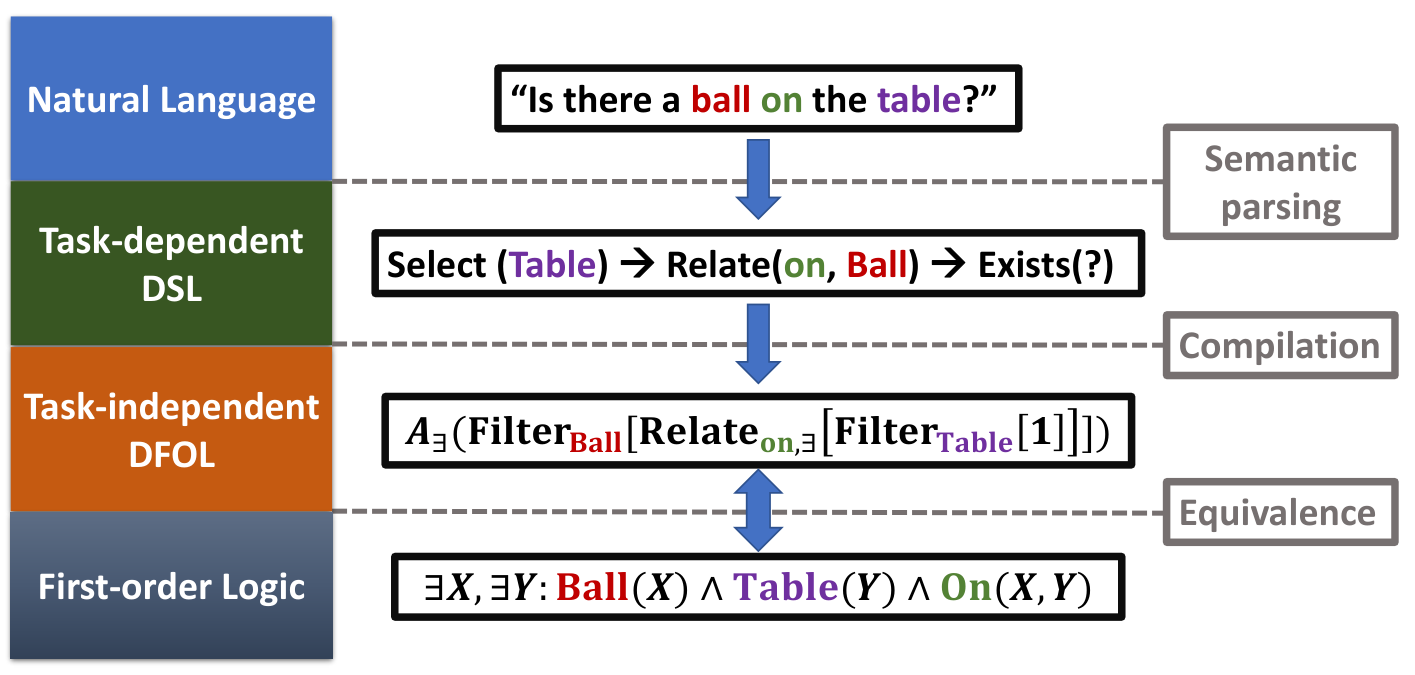
Our language system defines the pipeline to translate the questions in the natural language (NL) all the way to the DFOL language which we can then run to find the answer to the question. However, as opposed to many similar frameworks in the literature, our translation process takes place in two steps. First, we parse the NL question into the task-dependent, high-level, domain-specific language (DSL) of the target task. We then compile the resulted DSL program into the task-independent, low-level DFOL language. This separation is important because the $\nabla$-FOL core reasoning engine executes the task-independent, four basic operators of the DFOL language (i.e. Filter, Relate, Neg and $\mathcal{A}_{\{\forall,\exists,\nexists\}}$) and not the task specific DSL operators. This distinguishes $\nabla$-FOL from similar frameworks in the literature as a general-purpose formalism; that is, $\nabla$-FOL can cover any reasoning task that is representable via first-order logic, and not just a specific DSL. This is mainly due to the fact that DFOL programs are equivalent to FOL formulas (up to reordering) as shown in Section 3.3. Figure 3 shows the proposed language system along with its different levels of abstraction. For more details, please refer to our PyTorch code base: https://github.com/microsoft/DFOL-VQA.

For the GQA task, we train a neural semantic parser using the annotated programs in the dataset to accomplish the first step of translation. For the second step, we simply use a compiler, which converts each high-level GQA operator into a composition of DFOL basic operators. Table 4 shows this (fixed) conversion along with the equivalent FOL formula for each GQA operator.

Most operators in the GQA DSL are parameterized by a set of NL tokens that specify the arguments of the operation (e.g. "attr" in GFilter specifies the attribute that the operator is expected to filter the objects based upon). In addition to the NL arguments, both terminal and non-terminal operators take as input the attention vector(s) on the objects present in the scene (except for GSelect which does not take any input attention vector). However, in terms of their outputs, terminal and non-terminal operators are fundamentally different. A terminal operator produces a scalar likelihood or a list of scalar likelihoods (for "query" type operators). Because they are "terminal", terminal operators have logical quantifiers in their FOL description; this, in turn, prompts the aggregation operator $\mathcal{A}_{\{\forall,\exists,\nexists\}}$ in their equivalent DFOL translation. Non-terminal operators, on the other hand, produce attention vectors on the objects in the scene without calculating the aggregated likelihood.

Appendix C: Some Examples from the Hard and the Easy Sets

In this appendix, we visually demonstrate a few examples from the hard and the easy subsets of the GQA Test-Dev split. Figures 4,5,6 show a few examples from the hard set with their corresponding questions, while Figures 7,8 show a few examples from the easy set. In these examples, the green rectangles represent where in the image the model is attending according to the attention vector $\bm{\alpha}(\mathcal{F}\mid X)$. Here the formula $\mathcal{F}$ represents either the entire question for the easy set examples or the partial question up until to the point where the visual system failed to produce correct likelihoods for the hard set examples. We have included the exact nature of the visual system’s failure for the hard set examples in the captions. As illustrated in the paper, the visually hard-easy division here is with respect to the original Faster-RCNN featurization. This means that the "hard" examples presented here are not necessarily impossible in general, but are hard with respect to this specific featurization.

Furthermore, in Figure 9, we have demonstrated two examples from the hard set for which taking into the consideration the context of the question via the calibration process helped to overcome the imperfectness of the visual system and find the correct answer. Please refer to the caption for the details.

(a)

(b)

Figure 4: Hard Set: (a) Q: "What are the rackets are lying on the top of?" As the attention bounding boxes show, the visual system has a hard time detecting the rackets in the first place and as a result is not able to reason about the rest of the question. (b) Q: "Does the boy’s hair have short length and white color?" In this example, the boy’s hair are not even visible, so even though the model can detect the boy, it cannot detect his hair and therefore answer the question correctly.

(a)

(b)

Figure 5: Hard Set: (a) Q: "What is the cup made of?" As the attention bounding boxes show, the visual system has a hard time finding the actual cups in the first place as they are pretty blurry. (b) Q: "The open umbrella is of what color?" In this example, the visual system was in fact able to detect an object that is both "umbrella" and "open" but its color is ambiguous and can be classified as "black" even by the human eye. However, the ground truth answer is "blue" which is hard to see visually.

(a)

(b)

Figure 6: Hard Set: (a) Q: "What are the pieces of furniture in front of the staircase?" In this case, the model has a hard time detecting the staircase in the scene in the first place and therefore cannot find the correct answer. (b) Q: "What’s the cat on?" In this example, the visual system can in fact detect the cat and supposedly the object that cat is "on"; however, it cannot infer the fact that there is actually a laptop keyboard invisible between the cat and the desk.

(a)

(b)

Figure 7: Easy Set: (a) Q: "Does that shirt have red color?" (b) Q: "Are the glass windows round and dark?"

(a)

(b)

Figure 8: Easy Set: (a) Q: "What side of the photo is umpire on?" (b) Q: "Are the sandwiches to the left of the napkin triangular and soft?"

(a)

(b)

Figure 9: (a) Q: "Are there any lamps next to the books on the right?" Due to the similar color of the lamp with its background, the visual oracle assigned a low probability for the predicate ’lamp’ which in turn pushes the answer likelihood below $0.5$. The calibration, however, was able to correct this by considering the context of ’books’ in the image. (b) Q: "Is the mustard on the cooked meat?" In this case, the visual oracle had a hard time recognizing the concept of ’cooked’ which in turn pushes the answer likelihood below $0.5$. The calibration, however, was able to alleviate this by considering the context of ’mustard’ and ’meat’ in the visual input and boosts the overall likelihood.

References

- Agrawal et al. (2016) Agrawal, A., Batra, D., and Parikh, D. Analyzing the behavior of visual question answering models. arXiv preprint arXiv:1606.07356, 2016.
- Agrawal et al. (2018) Agrawal, A., Batra, D., Parikh, D., and Kembhavi, A. Don’t just assume; look and answer: Overcoming priors for visual question answering. In Proceedings of the IEEE Conference on Computer Vision and Pattern Recognition, pp. 4971–4980, 2018.
- Amizadeh et al. (2018) Amizadeh, S., Matusevych, S., and Weimer, M. Learning to solve circuit-sat: An unsupervised differentiable approach. In International Conference on Learning Representations, 2018.
- Amizadeh et al. (2019) Amizadeh, S., Matusevych, S., and Weimer, M. Pdp: A general neural framework for learning constraint satisfaction solvers. arXiv preprint arXiv:1903.01969, 2019.
- Anderson et al. (2018) Anderson, P., He, X., Buehler, C., Teney, D., Johnson, M., Gould, S., and Zhang, L. Bottom-up and top-down attention for image captioning and visual question answering. In Proceedings of the IEEE conference on computer vision and pattern recognition, pp. 6077–6086, 2018.
- Andreas et al. (2016) Andreas, J., Rohrbach, M., Darrell, T., and Klein, D. Neural module networks. In Proceedings of the IEEE Conference on Computer Vision and Pattern Recognition, pp. 39–48, 2016.
- Antol et al. (2015) Antol, S., Agrawal, A., Lu, J., Mitchell, M., Batra, D., Lawrence Zitnick, C., and Parikh, D. VQA: Visual question answering. In Proceedings of the IEEE international conference on computer vision, pp. 2425–2433, 2015.
- Cai et al. (2017) Cai, J., Shin, R., and Song, D. Making neural programming architectures generalize via recursion. arXiv preprint arXiv:1704.06611, 2017.
- Chen et al. (2020) Chen, X., Liang, C., Yu, A. W., Zhou, D., Song, D., and Le, Q. Neural symbolic reader: Scalable integration of distributed and symbolic representations for reading comprehension. In International Conference on Learning Representations, 2020. URL https://openreview.net/forum?id=ryxjnREFwH.
- Garcez et al. (2019) Garcez, A. d., Gori, M., Lamb, L. C., Serafini, L., Spranger, M., and Tran, S. N. Neural-symbolic computing: An effective methodology for principled integration of machine learning and reasoning. arXiv preprint arXiv:1905.06088, 2019.
- Goyal et al. (2017) Goyal, Y., Khot, T., Summers-Stay, D., Batra, D., and Parikh, D. Making the V in VQA matter: Elevating the role of image understanding in visual question answering. In Proceedings of the IEEE Conference on Computer Vision and Pattern Recognition, pp. 6904–6913, 2017.
- Gulwani et al. (2017) Gulwani, S., Polozov, O., Singh, R., et al. Program synthesis. Foundations and Trends® in Programming Languages, 4(1-2):1–119, 2017.
- Huang et al. (2015) Huang, Z., Xu, W., and Yu, K. Bidirectional LSTM-CRF models for sequence tagging. arXiv preprint arXiv:1508.01991, 2015.
- Hudson & Manning (2019a) Hudson, D. and Manning, C. D. Learning by abstraction: The neural state machine. In Advances in Neural Information Processing Systems, pp. 5901–5914, 2019a.
- Hudson & Manning (2018) Hudson, D. A. and Manning, C. D. Compositional attention networks for machine reasoning. arXiv preprint arXiv:1803.03067, 2018.
- Hudson & Manning (2019b) Hudson, D. A. and Manning, C. D. GQA: A new dataset for real-world visual reasoning and compositional question answering. In Proceedings of the IEEE Conference on Computer Vision and Pattern Recognition, pp. 6700–6709, 2019b.
- Johnson et al. (2017) Johnson, J., Hariharan, B., van der Maaten, L., Fei-Fei, L., Lawrence Zitnick, C., and Girshick, R. Clevr: A diagnostic dataset for compositional language and elementary visual reasoning. In Proceedings of the IEEE Conference on Computer Vision and Pattern Recognition, pp. 2901–2910, 2017.
- Kull et al. (2017) Kull, M., Silva Filho, T., and Flach, P. Beta calibration: a well-founded and easily implemented improvement on logistic calibration for binary classifiers. In Artificial Intelligence and Statistics, pp. 623–631, 2017.
- Lee et al. (2019) Lee, K., Palangi, H., Chen, X., Hu, H., and Gao, J. Learning visual relation priors for image-text matching and image captioning with neural scene graph generators. abs/1909.09953, 2019. URL http://arxiv.org/abs/1909.09953.
- Li et al. (2019) Li, G., Duan, N., Fang, Y., Gong, M., Jiang, D., and Zhou, M. Unicoder-VL: A universal encoder for vision and language by cross-modal pre-training. arXiv preprint arXiv:1908.06066, 2019.
- Liang et al. (2016) Liang, C., Berant, J., Le, Q., Forbus, K. D., and Lao, N. Neural symbolic machines: Learning semantic parsers on freebase with weak supervision. arXiv preprint arXiv:1611.00020, 2016.
- Liang (2016) Liang, P. Learning executable semantic parsers for natural language understanding. Communications of the ACM, 59(9):68–76, 2016.
- Lu et al. (2019) Lu, J., Batra, D., Parikh, D., and Lee, S. Vilbert: Pretraining task-agnostic visiolinguistic representations for vision-and-language tasks. In Advances in Neural Information Processing Systems, pp. 13–23, 2019.
- Mao et al. (2019) Mao, J., Gan, C., Kohli, P., Tenenbaum, J. B., and Wu, J. The neuro-symbolic concept learner: Interpreting scenes, words, and sentences from natural supervision. arXiv preprint arXiv:1904.12584, 2019.
- Neelakantan et al. (2015) Neelakantan, A., Le, Q. V., and Sutskever, I. Neural programmer: Inducing latent programs with gradient descent. arXiv preprint arXiv:1511.04834, 2015.
- Neelakantan et al. (2016) Neelakantan, A., Le, Q. V., Abadi, M., McCallum, A., and Amodei, D. Learning a natural language interface with neural programmer. arXiv preprint arXiv:1611.08945, 2016.
- Parisotto et al. (2016) Parisotto, E., Mohamed, A.-r., Singh, R., Li, L., Zhou, D., and Kohli, P. Neuro-symbolic program synthesis. arXiv preprint arXiv:1611.01855, 2016.
- Pennington et al. (2014) Pennington, J., Socher, R., and Manning, C. D. GloVe: Global vectors for word representation. In Empirical Methods in Natural Language Processing (EMNLP), pp. 1532–1543, 2014. URL http://www.aclweb.org/anthology/D14-1162.
- Pierrot et al. (2019) Pierrot, T., Ligner, G., Reed, S. E., Sigaud, O., Perrin, N., Laterre, A., Kas, D., Beguir, K., and de Freitas, N. Learning compositional neural programs with recursive tree search and planning. In Advances in Neural Information Processing Systems, pp. 14646–14656, 2019.
- Platt (2000) Platt, J. Probabilities for SV machines. advances in large margin classifiers (pp. 61–74), 2000.
- Ray et al. (2016) Ray, A., Christie, G., Bansal, M., Batra, D., and Parikh, D. Question relevance in VQA: identifying non-visual and false-premise questions. arXiv preprint arXiv:1606.06622, 2016.
- Reed & De Freitas (2015) Reed, S. and De Freitas, N. Neural programmer-interpreters. arXiv preprint arXiv:1511.06279, 2015.
- Ren et al. (2015) Ren, S., He, K., Girshick, R., and Sun, J. Faster R-CNN: Towards real-time object detection with region proposal networks. In Advances in neural information processing systems, pp. 91–99, 2015.
- Saha et al. (2019) Saha, A., Ansari, G. A., Laddha, A., Sankaranarayanan, K., and Chakrabarti, S. Complex program induction for querying knowledge bases in the absence of gold programs. Transactions of the Association for Computational Linguistics, 7:185–200, March 2019. doi: 10.1162/tacl_a_00262. URL https://www.aclweb.org/anthology/Q19-1012.
- Selsam et al. (2018) Selsam, D., Lamm, M., Bünz, B., Liang, P., de Moura, L., and Dill, D. L. Learning a sat solver from single-bit supervision. arXiv preprint arXiv:1802.03685, 2018.
- Selvaraju et al. (2020) Selvaraju, R. R., Tendulkar, P., Parikh, D., Horvitz, E., Ribeiro, M., Nushi, B., and Kamar, E. SQuINTing at VQA Models: Interrogating VQA Models with Sub-Questions. arXiv preprint arXiv:2001.06927, 2020.
- Serafini & Garcez (2016) Serafini, L. and Garcez, A. d. Logic tensor networks: Deep learning and logical reasoning from data and knowledge. arXiv preprint arXiv:1606.04422, 2016.
- Shi et al. (2019) Shi, J., Zhang, H., and Li, J. Explainable and explicit visual reasoning over scene graphs. In Proceedings of the IEEE Conference on Computer Vision and Pattern Recognition, pp. 8376–8384, 2019.
- Socher et al. (2013) Socher, R., Chen, D., Manning, C. D., and Ng, A. Reasoning with neural tensor networks for knowledge base completion. In Advances in neural information processing systems, pp. 926–934, 2013.
- Tan & Bansal (2019) Tan, H. and Bansal, M. LXMERT: Learning cross-modality encoder representations from transformers. arXiv preprint arXiv:1908.07490, 2019.
- van Krieken et al. (2020) van Krieken, E., Acar, E., and van Harmelen, F. Analyzing differentiable fuzzy logic operators. arXiv preprint arXiv:2002.06100, 2020.
- Vedantam et al. (2019) Vedantam, R., Desai, K., Lee, S., Rohrbach, M., Batra, D., and Parikh, D. Probabilistic neural-symbolic models for interpretable visual question answering. arXiv preprint arXiv:1902.07864, 2019.
- Xu et al. (2018) Xu, J., Zhang, Z., Friedman, T., Liang, Y., and Broeck, G. A semantic loss function for deep learning with symbolic knowledge. In International Conference on Machine Learning, pp. 5502–5511, 2018.
- Yang et al. (2018) Yang, J., Lu, J., Lee, S., Batra, D., and Parikh, D. Graph R-CNN for scene graph generation. In Proceedings of the European conference on computer vision (ECCV), pp. 670–685, 2018.
- Yi et al. (2018) Yi, K., Wu, J., Gan, C., Torralba, A., Kohli, P., and Tenenbaum, J. Neural-symbolic VQA: Disentangling reasoning from vision and language understanding. In Advances in Neural Information Processing Systems, pp. 1031–1042, 2018.
- Zellers et al. (2018) Zellers, R., Yatskar, M., Thomson, S., and Choi, Y. Neural motifs: Scene graph parsing with global context. In Proceedings of the IEEE Conference on Computer Vision and Pattern Recognition, pp. 5831–5840, 2018.
- Zellers et al. (2019) Zellers, R., Bisk, Y., Farhadi, A., and Choi, Y. From recognition to cognition: Visual commonsense reasoning. In Proceedings of the IEEE Conference on Computer Vision and Pattern Recognition, pp. 6720–6731, 2019.
- Zhou et al. (2015) Zhou, B., Tian, Y., Sukhbaatar, S., Szlam, A., and Fergus, R. Simple baseline for visual question answering. arXiv preprint arXiv:1512.02167, 2015.
- Zhou et al. (2020) Zhou, L., Palangi, H., Zhang, L., Hu, H., Corso, J. J., and Gao, J. Unified vision-language pre-training for image captioning and VQA. AAAI, 2020.