Convex Relaxation of Combined Heat
and Power Dispatch

Abstract

Combined heat and power dispatch promotes interactions and synergies between electric power systems and district heating systems. However, nonlinear and nonconvex heating flow imposes significant challenges on finding qualified solutions efficiently. Most existing methods rely on constant flow assumptions to derive a linear heating flow model, sacrificing optimality for computational simplicity. This paper proposes a novel convex combined heat and power dispatch model based on model simplification and constraint relaxation, which improves solution quality and avoids assumptions on operating regimes of district heating systems. To alleviate mathematical complexity introduced by the commonly used node method, a simplified thermal dynamic model is proposed to capture temperature changes in networked pipelines. Conic and polyhedral relaxations are then applied to convexify the original problems with bilinear and quadratic equality constraints. Furthermore, an adaptive solution algorithm is proposed to successively reduce relaxation gaps based on dynamic bivariate partitioning, improving solution optimality with desirable computational efficiency. The proposed method is verified on a 33-bus electric power system integrated with a 30-node district heating system and compared to nonlinear programming solvers and constant-flow-based solutions.

I Introduction

Increasing deployment of combined heat and power plants (CHP) and heat pumps intensifies energy interactions between electric power systems (EPS) and district heating systems (DHS) [1, 2]. Combined heat and power dispatch (CHPD) is utilized for coordinated scheduling of interdependent electricity and heat systems, which promotes a minimization of operational costs and enhances renewable energy utilization [3, 4].

In many parts of the world, heat is generated and supplied in a centralized way through networked pipelines with higher efficiency and less pollution, such as in North China and Europe [5]. Thus, the process of water distribution and heat delivery needs to be modeled in CHPD. A combined analysis of electric power and heating flow is studied in [6] based on static hydraulic-thermal conditions of DHS [7]. Network-constrained heating flow is incorporated into the simulation model, while time delays and temperature dynamics of heat distribution are not fully considered [6]. Thermal dynamics in DHS are investigated in [8] based on the so-called node method [9], which captures the correlation of nodal temperature at different time steps. Thermal storage and network flexibility of DHS in CHPD are further explored in [10, 11, 12, 13] for cost reduction and integration of renewable power.

One basic challenge so far is that nonlinear and nonconvex network flow renders CHPD problems hard to solve precisely and efficiently. Mathematically speaking, the CHPD problem considering electric power flow and district heating flow is of nonconvex nonlinear programming (NLP) or mixed-integer nonlinear programming type, for which it is quite difficult to obtain optimal solutions within limited time [14]. Available approaches with respect to CHPD can be briefly categorized into two groups: heuristic iterative algorithms [15, 8] or model assumptions [10].

In general, heuristic algorithms solve the CHPD problem by either metaheuristics or customized iterations. Reference [16] provides a review of metaheuristics implemented in optimal scheduling of power and heat generation, including particle swarm optimization [15], gravitational search algorithm, and so on. However, theses metaheuristics do not include complex heating flow as model constraints. On the other hand, some solution algorithms use iterative strategies by fixing time delays of heat delivery [8] or mass flow rates [17] in each iteration. These iterative strategies can obtain desired solutions by tuning relevant parameters to appropriate values. However, they tend to be specified for certain scenarios and rely on extensive experience in designing a viable strategy. Besides, some existing algorithms [8] rely on general NLP solvers (such as IPOPT [18]) to produce a candidate solution if both mass flow rates and nodal temperatures in the DHS are set as decision variables. NLP solvers based on interior point methods only aim to find local solutions for nonconvex problems, and may have unsatisfactory performance. Another commonly used method for CHPD employs model assumptions, where DHS is simplified to the constant-flow mode [10, 19]. As a consequence, the computational complexity is significantly reduced since the heating flow model is linear under the constant-flow assumption. However, this approach obviously sacrifices optimality for computing simplicity, since many candidate solutions are potentially eliminated from the solution space.

Reduction in operational costs may save considerable amount of money depending on the system size. Therefore, it is critical to improve the solution quality and computational performance for CHPD. To this end, a convex CHPD model is proposed based on model simplification and constraint relaxation in this paper. The proposed convex model is designed for general CHPD problems without any assumptions on operating regimes. Convexity guarantees that a globally optimal solution with respect to the relaxed CHPD model can be found efficiently. In particular, a simplified thermal dynamic (STD) model is developed to depict temperature changes in the DHS, avoiding introducing numerous integer variables that is required to setup temperature correlation for the node method. Conic and polyhedral relaxations are then utilized to relax nonconvex quadratic equality constraints and bilinear constraints. The convex CHPD model is not equivalent to the original problem, since relaxation enlarges the original nonconvex feasible set until it is convex. It is thus critical to derive a tight relaxation to improve the solution quality. Here, an adaptive solution algorithm is established to enhance the relaxation quality based on dynamic bivariate partitioning and piecewise McCormick envelopes [20]. Variable domains pertaining to bilinear terms are sequentially divided into a given number of partitions to reduce the size of relaxed feasible regions. Instead of uniformly partitioning domains of all variables, the adaptive strategy identifies bilinear constraints that are most significantly violated and iteratively add incremental partitions to avoid introducing too many binary variables. Thus, the relaxation quality can be strengthened successively with satisfactory computational efficiency. Numerical experiments on a test system composed of a 33-bus EPS and a 30-node DHS validate the effectiveness of the proposed method in terms of solution quality and computational feasibility.

To the authors’ best knowledge, this is the first paper investigating convex optimization and solution algorithms for general CHPD problems. The main contributions are summarized as follows: 1) A novel convex CHPD model is proposed without assumptions on constant mass flow rates. The model jointly optimizes operational strategies for EPS and DHS with satisfactory computational efficiency and improved solution quality; 2) A simplified thermal dynamic model is developed to characterize temperature changes in heating networks, mitigating the mathematical complexity of the node method. 3) Both conic and polyhedral relaxations are implemented in the convex CHPD model with thorough modeling of hydraulic and thermal conditions in the DHS. 4) A novel adaptive solution algorithm is devised based on dynamic bivariate partitioning and piecewise polyhedral relaxation to reduce relaxation gaps while preserving computational efficiency.

II Mathematical Model of CHPD

II-A Electric Power System

Considering the limited size of DHS, electric power distribution systems are modeled here with different types of distributed generators, including gas-fired generators, combined heat and power plants, photovoltaic panels, and wind turbines. Electricity is consumed by end-users and electrical devices, e.g., water pumps and heat pumps. Active and reactive nodal power injections $P_{j,t}$ and $Q_{j,t}$ from bus $j$ at time $t$ are expressed as

$$\begin{aligned} P_{j,t}=&\sum_{g\in\mathcal{G}_{j}}P_{g,t}^{\mathrm{G}}+\sum_{c\in\mathcal{C}_{j}}P_{c,t}^{\mathrm{C}}+\sum_{p\in\mathcal{P}_{j}}P_{p,t}^{\mathrm{PV}}+\sum_{w\in\mathcal{W}_{j}}P_{w,t}^{\mathrm{WT}}-\\ &\sum_{(k,l)\in\mathcal{B}_{j}^{\mathrm{WP}}}P_{kl,t}^{\mathrm{WP}}-\sum_{h\in\mathcal{H}_{j}}P_{h,t}^{\mathrm{HP}}-P_{j,t}^{\mathrm{D}},\forall j\in\mathcal{J},\end{aligned}$$ (1)

$$\begin{aligned} Q_{j,t}=&\sum_{g\in\mathcal{G}_{j}}Q_{g,t}^{\mathrm{G}}+\sum_{c\in\mathcal{C}_{j}}Q_{c,t}^{\mathrm{C}}+\sum_{p\in\mathcal{P}_{j}}Q_{p,t}^{\mathrm{PV}}+\\ &\sum\nolimits_{w\in\mathcal{W}_{j}}Q_{w,t}^{\mathrm{WT}}-Q_{j,t}^{\mathrm{D}},\forall j\in\mathcal{J},\end{aligned}$$ (2)

where $P_{g,t}^{\mathrm{G}}$, $P_{c,t}^{\mathrm{C}}$, $P_{p,t}^{\mathrm{PV}}$ and $P_{w,t}^{\mathrm{WT}}$ denote active power of the $g$-th generator and the $c$-th CHP, and forecasted power from the photovoltaic array and the wind turbine [21], respectively; $P_{kl,t}^{\mathrm{WP}}$ and $P_{h,t}^{\mathrm{HP}}$ are active power consumed by the water pump located at pipe $(k,l)$ in DHS and the $h$-th heat pump, respectively; symbols for reactive power are represented by $Q$ with corresponding superscripts and subscripts; $\mathcal{J}$ refers to the set of buses in the electric power network; $\mathcal{G}_{j}$, $\mathcal{C}_{j}$, $\mathcal{P}_{j}$, $\mathcal{W}_{j}$, and $\mathcal{H}_{j}$ are sets of generators, CHP, photovoltaic panels, wind turbines, and heat pumps that are connected to bus $j$, respectively; $\mathcal{B}_{j}^{\mathrm{WP}}$ is the set of pipes in DHS with installation of water pumps that couple with bus $j$ in EPS.

The branch flow model is adopted to model power flow in radial distribution feeders. Nonlinear AC power flow models are transformed to tractable convex models using angle relaxation and conic relaxation [22, 23]. Active and reactive power flow equations at bus $j$ in EPS are given as

$$P_{j,t}=\sum_{k:j\rightarrow k}P_{jk,t}-\sum_{i:i\rightarrow j}\left(P_{ij,t}-r_{ij}l_{ij,t}\right),\forall j\in\mathcal{J},$$ (3)

$$Q_{j,t}=\sum_{k:j\rightarrow k}Q_{jk,t}-\sum_{i:i\rightarrow j}\left(Q_{ij,t}-x_{ij}l_{ij,t}\right),\forall j\in\mathcal{J},$$ (4)

where $P_{ij,t}$ and $Q_{ij,t}$ are active and reactive power at bus $i$ flowing towards bus $j$ at time $t$, respectively; $r_{ij}$ and $x_{ij}$ are resistance and reactance of branch $(i,j)$, respectively; $l_{ij,t}$ refers to the squared magnitude of the branch current. Branch power flow defined by nodal voltages and currents are indicated as

$$v_{j,t}\!=\!v_{i,t}\!-\!2\left(\!r_{ij}\!P_{ij,t}\!+\!x_{ij}\!Q_{ij,t}\!\right)\!+\!\left(r_{ij}^{2}\!+\!x_{ij}^{2}\right)\!l_{ij,t},\!\forall(i,j)\!\in\!\mathcal{E},$$ (5)

$$\left\|\begin{array}[]{c}{2P_{ij,t}},{2Q_{ij,t}},{l_{ij,t}-v_{i,t}}\end{array}\right\|_{2}\leq l_{ij,t}+v_{i,t},\forall(i,j)\in\mathcal{E},$$

where $v_{i,t}$ denotes the squared voltage magnitude at bus $i$; $\mathcal{E}$ refers to the set of branches in EPS. Boundary constraints on electric power generation and consumption are expressed as

$$\underline{P}_{g}^{\mathrm{G}}\leq P_{g,t}^{\mathrm{G}}\leq\bar{P}_{g}^{\mathrm{G}},\underline{Q}_{g}^{\mathrm{G}}\leq Q_{g,t}^{\mathrm{G}}\leq\bar{Q}_{g}^{\mathrm{G}},\forall g\in\mathcal{G},$$ (7)

$$\underline{P}_{c}^{\mathrm{C}}\leq P_{c,t}^{\mathrm{C}}\leq\bar{P}_{c}^{\mathrm{C}},\underline{Q}_{c}^{\mathrm{C}}\leq Q_{c,t}^{\mathrm{C}}\leq\bar{Q}_{c}^{\mathrm{C}},\forall c\in\mathcal{C},$$ (8)

$$\underline{P}_{h}^{\mathrm{HP}}\leq P_{h,t}^{\mathrm{HP}}\leq\bar{P}_{h}^{\mathrm{HP}},\forall h\in\mathcal{H},$$ (9)

$$P_{p,t}^{\mathrm{PV}}\leq\bar{P}_{p,t}^{\mathrm{PV}},Q_{p,t}^{\mathrm{PV}}=0,\forall p\in\mathcal{P},$$ (10)

$$P_{w,t}^{\mathrm{WT}}\leq\bar{P}_{w,t}^{\mathrm{WT}},Q_{w,t}^{\mathrm{WT}}=\eta_{w}^{\mathrm{WT}}P_{w,t}^{\mathrm{WT}},\forall w\in\mathcal{W},$$ (11)

where $[\underline{P}_{g}^{\mathrm{G}},\bar{P}_{g}^{\mathrm{G}}]$, $[\underline{P}_{c}^{\mathrm{C}},\bar{P}_{c}^{\mathrm{C}}]$ and $[\underline{P}_{h}^{\mathrm{HP}},\bar{P}_{h}^{\mathrm{HP}}]$ are active power bounds of generators, CHP and heat pumps, respectively; $[\underline{Q}_{g}^{\mathrm{G}},\bar{Q}_{g}^{\mathrm{G}}]$ and $[\underline{Q}_{c}^{\mathrm{C}},\bar{Q}_{c}^{\mathrm{C}}]$ denote reactive power bounds of generators and CHP, respectively; $\eta_{w}^{\mathrm{WT}}$ refers to the reactive-active power ratio of wind turbines; $\mathcal{G}$, $\mathcal{C}$, $\mathcal{P}$, $\mathcal{W}$ and $\mathcal{H}$ are sets of generators, CHP, photovoltaic panels, wind turbines, and heat pumps, respectively. Ramping constraints are given as

$$\left|\Delta P_{g,t}^{\mathrm{G}}\right|\leq\Delta\bar{P}_{g}^{\mathrm{G}},\left|\Delta Q_{g,t}^{\mathrm{G}}\right|\leq\Delta\bar{Q}_{g}^{\mathrm{G}},\forall g\in\mathcal{G},$$ (12)

$$\left|\Delta P_{c,t}^{\mathrm{C}}\right|\leq\Delta\bar{P}_{c}^{\mathrm{C}},\left|\Delta Q_{c,t}^{\mathrm{C}}\right|\leq\Delta\bar{Q}_{c}^{\mathrm{C}},\forall c\in\mathcal{C},$$ (13)

$$\left|\Delta P_{h,t}^{\mathrm{HP}}\right|\leq\Delta\bar{P}_{h}^{\mathrm{HP}},\forall h\in\mathcal{H},$$ (14)

where $\Delta\bar{P}_{g,t}^{\mathrm{G}}$, $\Delta\bar{P}_{c,t}^{\mathrm{C}}$, and $\Delta\bar{P}_{h,t}^{\mathrm{HP}}$ are maximum ramping rates of active power for generators, CHP, heat pumps, respectively; $\Delta\bar{Q}_{g,t}^{\mathrm{G}}$ and $\Delta\bar{Q}_{c,t}^{\mathrm{C}}$ are reactive power ramping capability of generators and CHP, respectively. Limits on voltages and currents are given as

$$\underline{v}_{j}\leq v_{j,t}\leq\bar{v}_{j},\forall j\in\mathcal{J},l_{ij,t}\leq\bar{l}_{ij},\forall(i,j)\in\mathcal{E},$$ (15)

where $\underline{v}_{j}$ and $\bar{v}_{j}$ are squared lower and upper bounds of voltage magnitude; $\bar{l}_{ij}$ are squared maximum current magnitude.

II-B District Heating System

Modeling of DHS generally includes two sets of equations: hydraulic and thermal. Hydraulic equations focus on pressure conditions to determine the rate of heat delivery. Thermal equations characterize the changes in temperature levels within DHS.

Hydraulic dynamics are quickly transferred to the whole network within seconds, while temperature dynamics are quite slow [9]. Thus, mass flow rates and pressure conditions are calculated based on a static hydraulic model. Temperature changes are characterized using the dynamic approach.

II-B1 Hydraulic Model

Water flow in networked pipelines is assumed to be incompressible. Hence the distribution of mass flow is subject to continuity constraints, where the sum of incoming mass flow equals to the total outflow at each node, given as

$$m_{k,t}^{\mathrm{in}}-m_{k,t}^{\mathrm{out}}=\sum_{l:k\rightarrow l}m_{kl,t}-\sum_{j:j\rightarrow k}m_{jk,t},\forall k\in\mathcal{N},$$ (16)

where $m_{k,t}^{\mathrm{in}}$ and $m_{k,t}^{\mathrm{out}}$ indicate mass flow injection and outflow at node $k$, respectively; $m_{kl,t}$ denotes the mass flow rate in pipe $(k,l)$ at time $t$, and $m_{jk,t}$ represents the mass flow from node $j$ to node $k$; $\mathcal{N}$ is the set of nodes in DHS.

Water is distributed from points of high pressure to points of low pressure. Major pressure losses occur when water travels through pipelines due to friction against pipe walls. Minor pressure losses are induced by turbulence through fittings and appurtenances. The magnitude of major pressure losses is relevant to the water flow speed, internal roughness and pipe dimension, formulated as

$$p_{k,t}^{\mathrm{S}}-p_{l,t}^{\mathrm{S}}=\mu_{kl}m_{kl,t}^{2},p_{l,t}^{\mathrm{R}}-p_{k,t}^{\mathrm{R}}=\mu_{kl}m_{lk,t}^{2},\forall(k,l)\in\mathcal{B},$$ (17)

where $p_{k,t}^{\mathrm{S}}$ and $p_{k,t}^{\mathrm{R}}$ are supply and return pressure at node $k$, respectively; $\mathcal{B}$ is the set of pipes. The friction loss coefficient $\mu_{kl}$ can be derived based on dimensional analysis [24], given as

$$\mu_{kl}=f_{kl}^{\mathrm{D}}c_{\mathrm{Pa}}^{\mathrm{m}}\frac{8L_{kl}}{D_{kl}^{5}\rho_{\mathrm{w}}^{2}\pi^{2}g_{a}},f_{kl}^{\mathrm{D}}=\frac{1.325}{\left[\ln\left(\frac{\epsilon}{3.7D_{kl}}+\frac{5.74}{\operatorname{Re}^{0.9}}\right)\right]^{2}},$$ (18)

where $f_{kl}^{\mathrm{D}}$ is the Darcy-Weisbach friction factor; $c_{\mathrm{Pa}}^{\mathrm{m}}$ converts a pressure head (the height of water associated with its particular pressure, in units of meters) to a pressure (Pa); $L_{kl}$ and $D_{kl}$ are the pipe length and diameter, respectively; $\rho_{\mathrm{w}}$ denotes water density; $g_{a}$ is the gravitational acceleration constant; $\epsilon$ is the pipe internal roughness; $\operatorname{Re}$ is the Reynolds number [24]. Minor pressure losses are mainly induced by bends and reducers of heat-exchangers. Let $f_{k}^{\mathrm{m}}$ denote the minor loss coefficient, and $A_{k}$ be the cross-sectional area of heat-exchangers. Minor pressure losses are given by

$$p_{k,t}^{\mathrm{S}}-p_{k,t}^{\mathrm{R}}=\frac{f_{k}^{\mathrm{m}}c_{\mathrm{Pa}}^{\mathrm{m}}\left(m_{k,t}^{\text{out}}\right)^{2}}{2g_{a}\rho_{\mathrm{w}}^{2}A_{k}^{2}},\forall k\in\mathcal{N}.$$ (19)

Valves are installed in DHS for flow control or pressure regulation. Constraint (20) denotes pressure differentials provided by pressure-reducing valves at certain nodes, shown as

$$\Delta p_{kl,t}^{\mathrm{VL}}=p_{k,t}^{\mathrm{S}}-p_{l,t}^{\mathrm{S}},\Delta p_{kl,t}^{\mathrm{VL}}\geq 0,\forall(k,l)\in\mathcal{B}^{\mathrm{VL}},$$ (20)

where $\Delta p_{kl,t}^{\mathrm{VL}}$ is the pressure difference of the valve located at pipe $(k,l)$; $\mathcal{B}^{\mathrm{VL}}$ is the set of pipes with valves installed.

Water pumps raise potentials to overcome pressure losses in water distribution. Variable-speed electric centrifugal pumps are modeled here via the pump characteristic curve [25]. The relationship between the pressure difference and the flow rate is given as

$$p_{l,t}^{\mathrm{S}}\!-p_{k,t}^{\mathrm{S}}\!\!=\!c_{\mathrm{Pa}}^{\mathrm{m}}w_{kl,t}^{2}\!\!\left(\!\gamma_{kl}^{1}\!-\!\gamma_{kl}^{2}\!\left(\!\frac{m_{kl,t}}{\rho_{\mathrm{w}}w_{kl,t}}\!\right)^{\gamma_{kl}^{3}}\!\right)\!,\!\forall(k,\!l)\!\in\!\mathcal{B}^{\mathrm{WP}}\!\!,$$ (21)

where $w_{kl,t}$ indicates the relative pump speed; $\gamma_{kl}^{1}$, $\gamma_{kl}^{2}$, and $\gamma_{kl}^{3}$ are coefficients estimated through empirical data; $\mathcal{B}^{\mathrm{WP}}$ is the set of pipes with water pumps. Pump electric power is determined by

$$P_{kl,t}^{\mathrm{WP}}\!=\!\frac{m_{kl,t}\left(p_{l,t}^{\mathrm{S}}\!-\!p_{k,t}^{\mathrm{S}}\right)}{\eta_{kl}^{\mathrm{WP}}\rho_{\mathrm{w}}},P_{kl,t}^{\mathrm{WP}}\!\leq\!\bar{P}_{kl}^{\mathrm{WP}},\forall(k,l)\!\in\!\mathcal{B}^{\mathrm{WP}},$$ (22)

where $\eta_{kl}^{\mathrm{WP}}$ is the pump efficiency; $\bar{P}_{kl}^{\mathrm{WP}}$ denotes the electric power limit of water pumps. Constraints on nodal pressure and mass flow rates are indicated as

$$\underline{p}_{k}^{\mathrm{S}}\leq p_{k,t}^{\mathrm{S}}\leq\bar{p}_{k}^{\mathrm{S}},\underline{p}_{k}^{\mathrm{R}}\leq p_{k,t}^{\mathrm{R}}\leq\bar{p}_{k}^{\mathrm{R}},\forall k\in\mathcal{N},$$ (23)

$$\underline{m}_{kl}\leq m_{kl,t}\leq\bar{m}_{kl},\forall(k,l)\in\mathcal{B},$$ (24)

$$\underline{m}_{k}\leq m^{\mathrm{in}}_{k,t},m^{\mathrm{out}}_{k,t}\leq\bar{m}_{k},\forall k\in\mathcal{N},$$ (25)

where $[\underline{p}_{k}^{\mathrm{S}},\bar{p}_{k}^{\mathrm{S}}]$ and $[\underline{p}_{k}^{\mathrm{R}},\bar{p}_{k}^{\mathrm{R}}]$ denote pressure bounds in supply and return networks; $[\underline{m}_{kl},\bar{m}_{kl}]$ and $[\underline{m}_{k},\bar{m}_{k}]$ are mass flow limits.

II-B2 Thermal Model

Generated heat is shown as

$$H_{c,t}^{\mathrm{C}}=\eta_{c}^{\mathrm{C}}P_{c,t}^{\mathrm{C}},\forall c\in\mathcal{C},H_{h,t}^{\mathrm{HP}}=\eta_{h}^{\mathrm{HP}}P_{h,t}^{\mathrm{HP}},\forall h\in\mathcal{H},$$ (26)

where $H_{c,t}^{\mathrm{C}}$ and $H_{h,t}^{\mathrm{HP}}$ are heat produced by the $c$-th CHP and the $h$-th heat pump, respectively; $\eta_{c}^{\mathrm{C}}$ and $\eta_{h}^{\mathrm{HP}}$ represent the power-to-heat ratio of CHP and the coefficient of performance of a heat pump, respectively. Total heat is transferred to the heating network at heat sources and delivered to end-users at heat-exchangers, determined by the product of mass flow rates and temperatures rises (or drops). Heat flow at production and user sites satisfy

$$\sum_{c\in\mathcal{C}_{k}}\!H_{c,t}^{\mathrm{C}}\!+\!\sum_{h\in\mathcal{H}_{k}}\!H_{h,t}^{\mathrm{HP}}\!=\!c_{\mathrm{w}}m_{k,t}^{\mathrm{in}}\!\left(\!T_{k,t}^{\mathrm{S},\mathrm{in}}-T_{k,t}^{\mathrm{R}}\!\right)\!,\forall k\in\mathcal{N},$$ (27)

$$H_{k,t}^{\mathrm{D}}=c_{\mathrm{w}}m_{k,t}^{\mathrm{out}}\left(T_{k,t}^{\mathrm{S}}-T_{k,t}^{\mathrm{R},\mathrm{out}}\right),\forall k\in\mathcal{N},$$ (28)

where $T_{k,t}^{\mathrm{S},\mathrm{in}}$ and $T_{k,t}^{\mathrm{R}}$ are the supply temperature from the heat source at node $k$ and the nodal temperature at node $k$ in the return heating network, respectively; $T_{k,t}^{\mathrm{S}}$ and $T_{k,t}^{\mathrm{R},\mathrm{out}}$ denote the nodal temperatures at node $k$ in the supply network and the return temperatures from the heat user at node $k$, respectively; $H_{k,t}^{\mathrm{D}}$ refers to the heat load at node $k$ in DHS; $c_{\mathrm{w}}$ is the specific heat capacity of water; $\mathcal{C}_{k}$ and $\mathcal{H}_{k}$ are sets of CHP and heat pumps at node $k$.

We assume that all incoming water flow is fully mixed at each node. According to the law of energy conservation, the nodal temperature after mixing all incoming heating flow in the supply and return heating networks is determined by

$$T_{l,t}^{\mathrm{S}}=\frac{T_{l,t}^{\mathrm{S,in}}m_{l,t}^{\mathrm{in}}+\sum_{k:k\rightarrow l}T_{kl,t}^{\mathrm{S,out}}m_{kl,t}}{m_{l,t}^{\mathrm{in}}+\sum_{k:k\rightarrow l}m_{kl,t}},\forall l\in\mathcal{N},$$ (29)

$$T_{k,t}^{\mathrm{R}}=\frac{T_{k,t}^{\mathrm{R,out}}m_{k,t}^{\mathrm{out}}+\sum_{l:l\rightarrow k}T_{lk,t}^{\mathrm{R,out}}m_{lk,t}}{m_{k,t}^{\mathrm{out}}+\sum_{l:l\rightarrow k}m_{lk,t}},\forall k\in\mathcal{N},$$ (30)

where $T_{kl,t}^{\mathrm{S,out}}$ and $T_{lk,t}^{\mathrm{R,out}}$ are the outlet temperatures of pipe $(k,l)$ in supply and return networks, respectively. The correlation between pipeline inlet and nodal temperatures is given by

$$T_{kl,t}^{\mathrm{S,in}}=T_{k,t}^{\mathrm{S}},T_{lk,t}^{\mathrm{R,in}}=T_{l,t}^{\mathrm{R}},\forall(k,l)\in\mathcal{B},$$ (31)

where $T_{kl,t}^{\mathrm{S,in}}$ and $T_{lk,t}^{\mathrm{R,in}}$ are inlet temperature of pipe $(k,l)$ in supply and return networks, respectively.

Time delays of heat distribution are modeled by the node method [9]. In brief, the outlet temperature of a pipeline is defined as a nonlinear function of the inlet temperature at multiple previous time slots. The loss-free outlet temperature $\dot{T}_{kl,t}^{\mathrm{S,out}}$ of pipe $(k,l)$ in the supply network is formulated as

$$\dot{T}_{kl,t}^{\mathrm{S,out}}= \Big[(M_{kl,t}^{\mathrm{st}}-M_{kl})T_{kl,t-t_{kl,t}^{\mathrm{st}}}^{\mathrm{S,in}}+\Delta_{kl,t}^{\mathrm{S}}+$$ (32)

$$(m_{kl,t} \Delta t+M_{kl}-M_{kl,t}^{\mathrm{ed}})T_{kl,t-t_{kl,t}^{\mathrm{ed}}}^{\mathrm{S,in}}\Big]/\left(m_{kl,t}\Delta t\right),$$

where $\Delta t$ is the length of time step; time delays $t_{kl,t}^{\mathrm{st}}$ and $t_{kl,t}^{\mathrm{ed}}$ basically denote heat delivery time for hot water traveling through pipe $(k,l)$ at time $t$; $t_{kl,t}^{\mathrm{st}}$ can be regarded as the “arriving” time delay, while $t_{kl,t}^{\mathrm{ed}}$ is the “leaving” time delay, indicated as

$$t_{kl,t}^{\mathrm{st}}=\min\Bigg\{\zeta\geq 0;\sum_{\tau=t-\zeta}^{t}m_{kl,\tau}\Delta t>M_{kl}\Bigg\},$$ (33)

$$t_{kl,t}^{\mathrm{ed}}=\min\Bigg\{\zeta\geq 0;\sum_{\tau=t-\zeta}^{t}m_{kl,\tau}\Delta t>M_{kl}+m_{kl,t}\Delta t\Bigg\}.$$ (34)

Other auxiliary variables are formulated as

$$M_{kl}=\frac{\pi L_{kl}D_{kl}^{2}\rho_{\mathrm{w}}}{4},M_{kl,t}^{\mathrm{st}}=\sum_{\tau=t-t_{kl,t}^{\mathrm{st}}}^{t}m_{kl,\tau}\Delta t,$$ (35)

$$M_{kl,t}^{\mathrm{ed}}=\left\{\begin{aligned} &\sum_{\tau=t-t_{k,t}^{\mathrm{ed}}+1}^{t}m_{kl,\tau}\Delta t,t_{kl,t}^{\mathrm{ed}}>t_{kl,t}^{\mathrm{st}}\\ &M_{kl,t}^{\mathrm{st}},t_{kl,t}^{\mathrm{ed}}=t_{kl,t}^{\mathrm{st}}\end{aligned}\right.,$$ (36)

$$\Delta_{kl,t}^{\mathrm{S}}=\sum_{\tau=t-t_{kl,t}^{\mathrm{ed}}+1}^{t-t_{kl,t}^{\mathrm{st}}-1}m_{kl,\tau}\Delta tT_{kl,\tau}^{\mathrm{S,in}},$$ (37)

where $M_{kl}$ refers to the total mass of water in pipe $(k,l)$; $M_{kl,t}^{\mathrm{st}}$ and $M_{kl,t}^{\mathrm{ed}}$ are summations of water mass at different time instants. Considering heat losses appearing in water distribution, the outlet temperature $T_{kl,t}^{\mathrm{S,out}}$ of pipe $(k,l)$ at time $t$ is finally formulated as

$$T_{kl,t}^{\mathrm{S,out}}\!\!= T_{t}^{\mathrm{GD}}+\left(\dot{T}_{kl,t}^{\mathrm{S,out}}-T_{t}^{\mathrm{GD}}\right)\times$$ (38)

$$\text{exp}\left\{\!-\!\frac{\lambda_{kl}\Delta t}{A_{kl}\rho_{\mathrm{w}}c_{\mathrm{w}}}\left(t_{kl,t}^{\mathrm{st}}\!+\!\frac{1}{2}\!+\!\frac{M_{kl,t}^{\mathrm{ed}}-M_{kl,t}^{\mathrm{st}}}{m_{kl,t-t_{kl,t}^{\mathrm{st}}}\Delta t}\right)\right\},$$

where $T_{t}^{\mathrm{GD}}$ refers to the ground temperature; $\lambda_{kl}$ denotes the heat conductivity (W/m/K) of pipe $(k,l)$ in DHS. The heat distribution in the return network can be derived similarly. A visualized illustration can be found in [8].

Network constraints on nodal temperature in supply and return networks are denoted as

$$\underline{T}_{k}^{\mathrm{S}}\leq T_{k,t}^{\mathrm{S}},T_{k,t}^{\mathrm{S,in}}\leq\bar{T}_{k}^{\mathrm{S}},\underline{T}_{k}^{\mathrm{R}}\leq T_{k,t}^{\mathrm{R}},T_{k,t}^{\mathrm{R,out}}\leq\bar{T}_{k}^{\mathrm{R}},\forall k\in\mathcal{N},$$ (39)

where $[\underline{T}_{k}^{\mathrm{S}},\bar{T}_{k}^{\mathrm{S}}]$ and $[\underline{T}_{k}^{\mathrm{R}},\bar{T}_{k}^{\mathrm{R}}]$ are nodal temperature bounds in supply and return networks, respectively;

III Simplification and Relaxation

III-A Simplified Thermal Dynamic Model

As detailed from (32) to (38), the node method uses complex nonlinear equations (e.g., exponential terms in (38)) and logical conditions (e.g., time delays (33) and (34)) to characterize temperature dynamics and heat losses in DHS. The node method is accurate and easy to understand from the modeling perspective. However, it is computationally not affordable in optimization. For instance, the loss-free outlet temperature $\dot{T}_{kl,t}^{\mathrm{S,out}}$ is mapped with the inlet temperature $T_{kl,\tau}^{\mathrm{S,in}}$ at multiple time instants from $\tau=t-t^{\mathrm{ed}}_{kl,t}$ to $\tau=t-t^{\mathrm{st}}_{kl,t}$. Note that $t^{\mathrm{st}}_{kl,t}$ and $t^{\mathrm{ed}}_{kl,t}$ are both decision variables satisfying logic conditions in (33) and (34), and thus the temperature change equation (32) is “indeterminate”. To reformulate (32)-(34) as “exact” constraints in optimization, auxiliary integer variables are introduced based on the Big-M method [26]. The numbers of additional integer variables are proportional to the maximum time delay, the number of pipelines, and time periods.

To avoid the combinatorial inefficiency induced by logical constraints and auxiliary integer variables, the STD model is derived based on DHS dynamics. The partial differential equation capturing influence of flow speed and heat convection is given as [9]

$$\frac{\partial T}{\partial t}+\frac{m}{A\rho_{\mathrm{w}}}\frac{\partial T}{\partial x}+\frac{\lambda}{A\rho_{\mathrm{w}}c_{\mathrm{w}}}\left(T-T^{\mathrm{GD}}\right)=0,$$ (40)

where $T$ and $m$ denote temperature and mass flow rate, respectively; $T^{\mathrm{GD}}$ is the temperature of the surrounding ground; $\lambda$ refers to the thermal transfer coefficient (W/m/K). The partial derivatives are approximated using a first-order upwind scheme with respect to time $t$ and distance $x$. This discretization is applied to each pipeline at each time instant. Eventually, temperature dynamics in the supply heating network are modeled as

$$\frac{T_{kl,t}^{\mathrm{S}}-T_{kl,t-1}^{\mathrm{S}}}{\Delta t}+ \frac{m_{kl,t}}{A_{kl}\rho_{\mathrm{w}}}\frac{T_{kl,t}^{\mathrm{S,out}}-T_{kl,t}^{\mathrm{S,in}}}{L_{kl}}+$$ (41)

$$\frac{\lambda_{kl}}{A_{kl}\rho_{\mathrm{w}}c_{\mathrm{w}}}\left(T_{kl,t}^{\mathrm{S}}-T_{t}^{\mathrm{GD}}\right)=0,$$

where $T_{kl,t}^{\mathrm{S}}=(T_{kl,t}^{\mathrm{S,in}}+T_{kl,t}^{\mathrm{S,out}})/2$ refers to the average supply temperature of pipe $(k,l)$ at time $t$. Similarly, temperature dynamics in the return network are given by

$$\frac{T_{lk,t}^{\mathrm{R}}-T_{lk,t-1}^{\mathrm{R}}}{\Delta t}+ \frac{m_{lk,t}}{A_{kl}\rho_{\mathrm{w}}}\frac{T_{lk,t}^{\mathrm{R,out}}-T_{lk,t}^{\mathrm{R,in}}}{L_{kl}}+$$ (42)

$$\frac{\lambda_{kl}}{A_{kl}\rho_{\mathrm{w}}c_{\mathrm{w}}}\left(T_{lk,t}^{\mathrm{R}}-T_{t}^{\mathrm{GD}}\right)=0,$$

where $T_{lk,t}^{\mathrm{R}}=(T_{lk,t}^{\mathrm{R,out}}+T_{lk,t}^{\mathrm{R,in}})/2$ is the average return temperature of pipe $(k,l)$ at time $t$. The proposed STD model accounts for heat storage of pipes, heat losses to surroundings and time delays of heat distribution. Two set of equations (41) and (42) are incorporated into the CHPD model instead of (32)-(38) to enable a computationally efficient model.

III-B Conic and Polyhedral Relaxation

Nonconvex parts in the CHPD model mainly come from quadratic equality constraints and bilinear constraints. Quadratic equality constraints include pressure losses (17) and (19). Bilinear constraints are used in pump power equations (22), heat transfer equations (27) and (28), temperature mixing equations (29) and (30), and the STD model (41) and (42). The convex CHPD model is derived based on conic and polyhedral relaxations to form a second-order cone programming (SOCP) problem.

Quadratic equality constraints are reformulated as second-order cone constraints by replacing equal signs with inequality signs. Thus, major and minor pressure losses are reformulated as

$$p_{k,t}^{\mathrm{S}}-p_{l,t}^{\mathrm{S}}\geq\mu_{kl}m_{kl,t}^{2},p_{l,t}^{\mathrm{R}}-p_{k,t}^{\mathrm{R}}\geq\mu_{kl}m_{lk,t}^{2},\forall(k,l)\in\mathcal{B},$$ (43)

$$p_{k,t}^{\mathrm{S}}-p_{k,t}^{\mathrm{R}}\geq\frac{f_{k}^{\mathrm{m}}c_{\mathrm{Pa}}^{\mathrm{m}}\left(m_{k,t}^{\text{out}}\right)^{2}}{2g_{a}\rho_{\mathrm{w}}^{2}A_{k}^{2}},\forall k\in\mathcal{N}.$$ (44)

Bilinear constraints are relaxed based on polyhedral relaxation. Polyhedral relaxation provides an outer convex hull for bilinear terms based on McCormick envelopes, which retain linearity and minimizes the size of the relaxed feasible space. For instance, the heat transfer function (27) is reformulated as

$$\begin{aligned} H^{\mathrm{D}}_{k,t}\geq&c_{\mathrm{w}}\underline{m}_{k}(T^{\mathrm{S}}_{k,t}-T^{\mathrm{R,out}}_{k,t})+c_{\mathrm{w}}m^{\mathrm{in}}_{k,t}(\underline{T}^{\mathrm{S}}_{k}-\bar{T}^{\mathrm{R}}_{k})\\ &-c_{\mathrm{w}}\underline{m}_{k}(\underline{T}^{\mathrm{S}}_{k}-\bar{T}^{\mathrm{R}}_{k}),\end{aligned}$$ (45)

$$\begin{aligned} H^{\mathrm{D}}_{k,t}\geq&c_{\mathrm{w}}\bar{m}_{k}(T^{\mathrm{S}}_{k,t}-T^{\mathrm{R,out}}_{k,t})+c_{\mathrm{w}}m^{\mathrm{in}}_{k,t}(\bar{T}^{\mathrm{S}}_{k}-\underline{T}^{\mathrm{R}}_{k})\\ &-c_{\mathrm{w}}\bar{m}_{k}(\bar{T}^{\mathrm{S}}_{k}-\underline{T}^{\mathrm{R}}_{k}),\end{aligned}$$ (46)

$$\begin{aligned} H^{\mathrm{D}}_{k,t}\leq&c_{\mathrm{w}}\underline{m}_{k}(T^{\mathrm{S}}_{k,t}-T^{\mathrm{R,out}}_{k,t})+c_{\mathrm{w}}m^{\mathrm{in}}_{k,t}(\bar{T}^{\mathrm{S}}_{k}-\underline{T}^{\mathrm{R}}_{k})\\ &-c_{\mathrm{w}}\underline{m}_{k}(\bar{T}^{\mathrm{S}}_{k}-\underline{T}^{\mathrm{R}}_{k}),\end{aligned}$$ (47)

$$\begin{aligned} H^{\mathrm{D}}_{k,t}\geq&c_{\mathrm{w}}\bar{m}_{k}(T^{\mathrm{S}}_{k,t}-T^{\mathrm{R,out}}_{k,t})+c_{\mathrm{w}}m^{\mathrm{in}}_{k,t}(\underline{}{T}^{\mathrm{S}}_{k}-\bar{T}^{\mathrm{R}}_{k})\\ &-c_{\mathrm{w}}\bar{m}_{k}(\underline{}{T}^{\mathrm{S}}_{k}-\bar{T}^{\mathrm{R}}_{k}),\end{aligned}$$ (48)

where the bilinear constraint (27) is replaced by four linear inequality constraints (45)-(48). Polyhedral constraints for other bilinear constraints can be derived similarly.

In addition, the pump characteristic curve denoted as (21) is also nonconvex. However, the coefficient $\gamma^{3}_{kl}$ usually takes a value around 2 [25]. Thus, a convex operating region can be formulated for a water pump using quadratic inequality constraints. The relative pump speed $w_{kl,t}$ is eliminated by examining all possible values to form the operating region. Fig. 1 shows the convex operating region of a water pump with the $\gamma^{1}=99.02,\gamma^{2}=57.74,\gamma^{3}=2.156$. Red, blue and black dashed lines depict the pump characteristic curves when $w$ equals to 0.5, 0.75 and 1.0, respectively. The shaded area indicates the convex operating region of water pumps, expressed as

$$p_{l,t}^{\mathrm{S}}-p_{k,t}^{\mathrm{S}}\leq c_{\mathrm{Pa}}^{\mathrm{m}}\gamma_{kl}^{1}-c_{\mathrm{Pa}}^{\mathrm{m}}\gamma_{kl}^{2}\frac{m_{kl,t}^{2}}{\rho_{\mathrm{w}}^{2}},\forall(k,l)\in\mathcal{B}^{\mathrm{WP}}.$$ (49)

Fig. 1: Convex operating region of a water pump.

IV Relaxation Tightening

IV-A Piecewise Polyhedral Relaxation

The polyhedral relaxation based on McCormick envelopes is not tight if participating variables in bilinear terms are all continuous [27]. To improve the relaxation quality, McCormick envelopes are tightened via piecewise polyhedral relaxation. For the sake of brevity, the formulation for a general bilinear constraint $z=cxy$ with $(x,y)\in[\underline{x},\bar{x}]\times[\underline{y},\bar{y}]$ is given here, where $z$, $x$ and $y$ are decision variables, and $c$ refers to a constant. Without loss of generality, the domains of $x$ and $y$ are split into $n$ disjoint regions with identical segment lengths. Then, $2n$ binary variables are introduced, $\alpha_{i},\beta_{i},i\in\mathbb{I}_{1}^{n}$, to indicate which partitions in $x$ domain and $y$ domain are active. $\mathbb{I}_{a}^{b}$ refers to the set of integer variables from $a$ to $b$. Lower and upper bounds of $x$ and $y$ on the $i$-th partition ($i\in\mathbb{I}_{1}^{n}$) are calculated by

$$x_{i-1}=\underline{x}+(i-1)(\bar{x}-\underline{x})/n,x_{i}=\underline{x}+i(\bar{x}-\underline{x})/n,$$ (50)

$$y_{i-1}=\underline{y}+(i-1)(\bar{y}-\underline{y})/n,y_{i}=\underline{y}+i(\bar{y}-\underline{y})/n,$$ (51)

where $x_{i-1}$ and $x_{i}$ are lower and upper bounds of $x$ on the $i$-th partition; similarly, $y_{i-1}$ and $y_{i}$ are lower and upper bounds of $y$ on the $i$-th partition. A convex combination is used to formulate a piecewise polyhedral relaxation of bilinear equations, given as

$$x\!=\!\sum_{i=0}^{n}\!\sum_{j=0}^{n}\!\phi_{i,j}x_{i},y\!=\!\sum_{i=0}^{n}\!\sum_{j=0}^{n}\!\phi_{i,j}y_{j},z\!=\!\sum_{i=0}^{n}\!\sum_{j=0}^{n}\!\phi_{i,j}cx_{i}y_{j},$$ (52)

$$0\leq\phi_{i,j}\leq 1,\forall i\in\mathbb{I}_{0}^{n},\forall j\in\mathbb{I}_{0}^{n},$$ (53)

$$\sum_{i=1}^{n}\alpha_{i}=1,\sum_{i=1}^{n}\beta_{i}=1,\sum_{i=0}^{n}\sum_{j=0}^{n}\phi_{i,j}=1,$$ (54)

$$\phi_{0,j}\!\leq\!\alpha_{1},\phi_{i,j}\!\leq\!\alpha_{i}+\alpha_{i+1},\forall i\in\mathbb{I}_{1}^{n-1},\phi_{n,j}\!\leq\!\alpha_{n},\forall j\in\mathbb{I}_{0}^{n},$$ (55)

$$\phi_{i,0}\leq\beta_{1},\phi_{i,j}\leq\beta_{i}+\beta_{i+1},\forall j\in\mathbb{I}_{1}^{n-1},\phi_{i,n}\leq\beta_{n},\forall i\in\mathbb{I}_{0}^{n},$$ (56)

where $\phi_{i,j}$ is a continuous variable associated with the point of $(x_{i},y_{j},z_{i,j}=cx_{i}y_{j})$; binary variables $\alpha_{i}$ and $\beta_{j}$ are set to one if the $i$-th partition on the $x$ domain and the $j$-th partition on the $y$ domain are active. A detailed graphical illustration for the piecewise convex relaxation is given in Fig. 2, where the left-hand red box represents the active partition with $\alpha_{i}=1$ and $\beta_{j}=1$, namely, $x_{i-1}\leq x\leq x_{i}$ and $y_{j-1}\leq y\leq y_{j}$. The right side of Fig. 2 shows a convex polyhedral envelope for this particular partition.

Fig. 2: Illustration of piecewise polyhedral relaxation.

IV-B Adaptive Solution Algorithm

The piecewise polyhedral relaxation outlined above is introduced to tighten the McCormick envelopes based on mixed-integer second-order cone programming (MISOCP). In general, the more integer variables, the better the relaxation is due to a tighter outer approximation of the original feasible set. Conventional piecewise McCormick envelopes use uniform partitioning where piecewise relaxation occurs on all variable domains, leading to MISOCP problems with many binary variables. To promote a better relaxation without imposing a heavy computational burden, an adaptive solution algorithm is proposed based on dynamic bivariate partitioning to shrink the relaxed feasible region successively while balancing the computational requirement.

The main idea of the proposed adaptive strategy is to identify constraints with the highest violation and iteratively refine the domain partitions accordingly. Consequently, a sequence of MISOCP problems is solved based on a successively tighter piecewise polyhedral relaxation. The pseudocode for the adpative solution algorithm is reported in Algorithm 1. Suppose that the CHPD model has $m$ bilinear constraints, which can be generally formulated as $z_{i}=c_{i}x_{i}y_{i},i\in\mathbb{I}_{1}^{m}$. Each bilinear constraint is relaxed with $n_{i}$ partitions. The termination criterion is time limit $\bar{t}$.

Algorithm 1 The adaptive solution algorithm

1: Initialize $\bar{t}$ $\triangleright$ time limit

2: $n_{i}\leftarrow 1,\forall i\in\mathbb{I}_{1}^{m}$ $\triangleright$ numbers of partitions

3: $PreviousSolution\leftarrow$ NULL $\triangleright$ initialize a previous solution

4: $Tstart,Tend\leftarrow CurrentTime$

5: while $Tend-Tstart\leq\bar{t}$ do

6:    Implement piecewise relaxation based on (50)-(56) and $n_{i},i\in\mathbb{I}_{1}^{m}$

7:    Formulate a relaxed CHPD-MISOCP model

8:    Import $PreviousSolution$ as a warm start

9:    Solve the problem using Gurobi

10:    $PreviousSolution\leftarrow CurrentSolution$ $\triangleright$ save results

11:    Get solutions of bilinear terms as $x^{\ast}_{i},y^{\ast}_{i},z^{\ast}_{i},i\in\mathbb{I}_{1}^{m}$

12:    $\bar{gap}\leftarrow 0$, $I\leftarrow 1$

13:    for $i\in\mathbb{I}_{1}^{m}$ do

14:     $gap_{i}\leftarrow\frac{z^{\ast}_{i}-c_{i}x^{\ast}_{i}y^{\ast}_{i}}{z^{\ast}_{i}}\times 100\%$ $\triangleright$ constraint violation rate

15:     if $gap_{i}>\bar{gap}$ then

16:       $\bar{gap}\leftarrow gap_{i}$

17:       $I\leftarrow i$

18:     end if

19:    end for

20:    $n_{I}\leftarrow n_{I}+1$ $\triangleright$ refine partitions

21:    $Tend\leftarrow CurrentTime$ $\triangleright$ refresh run time

22: end while

Fig. 3 illustrates the main steps in the overall solution strategy. Model simplification and constraint relaxation are conducted first to derive a convex CHPD model. Then, two choices are offered depending on the operator preference. The reason is that integer variables generally increase computing efforts due to the exponential complexity for branching and bounding. Besides, solvers for MISOCP are also not as scalable as those for mixed-integer linear programming.

If system operators aim to find a feasible solution with limited time or computing resources, the convex CHPD model based on SOCP is solved to obtain a relaxed solution. A feasible solution with respect to the original CHPD problem is then recovered by fixing mass flow rates and re-optimizing the CHPD problem with known hydraulic conditions. On the other hand, if the solution optimality is the first concern instead of computing time, the CHPD model based on MISOCP is solved using the proposed adaptive algorithm. To effectively enhance the relaxation quality while balancing computational efforts, the adaptive strategy sequentially divides the domains of variables belonging to the most severely violated bilinear constraints into smaller partitions for tighter piecewise polyhedral relaxation. At each iteration, an updated CHPD model in MISOCP is formulated and solved to find a relaxed solution. Then, a feasible solution is determined according to the mass flow rates of the relaxed solution. Note that the previous solution can be saved to provide a warm start for solving the MISOCP problem in the next iteration, expediting the pruning and bounding process. The termination criteria can be tuned according to specific operator requirements, including a maximum count of iterations, a time limit, or a desirable objective bound to stop.

Fig. 3: Flowchart of the solution strategy for CHPD.

V Case Studies

V-A System Configuration

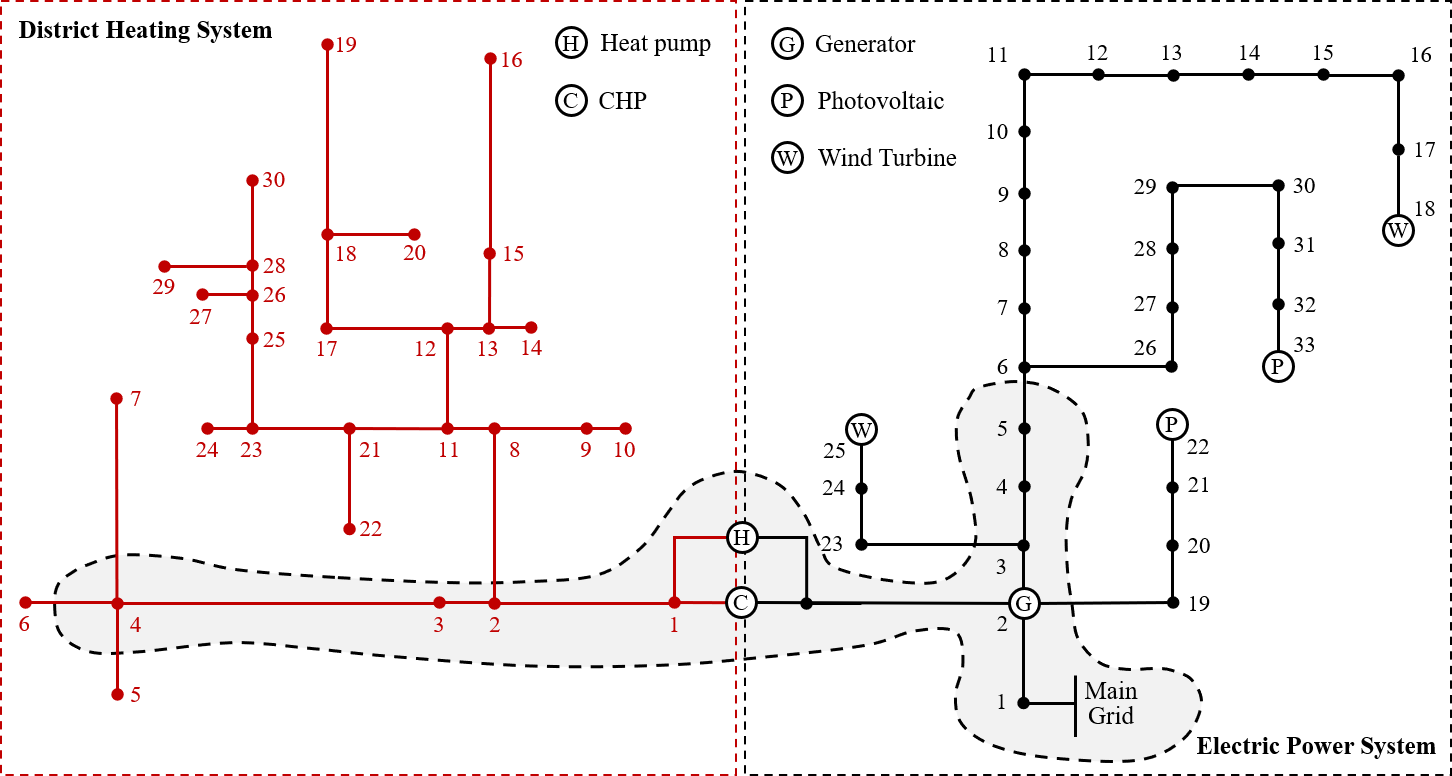
The proposed convex CHPD model and adaptive solution algorithm are tested on an integrated electricity and heat system, composed of a 33-bus 12.66 kV EPS [28] and a 30-node DHS [9]. Fig. 4 shows the test system with locations of the CHP, heat pump, gas-fired generator, wind turbines and photovoltaic arrays. The DHS contains 29 pipes and 17 heat-exchangers with a total length of 6.6 km. The peak electricity and heat loads are 3.72 MW and 11.44 MW, respectively.

Fig. 4: Diagram of the test integrated electricity and heat system.

V-B Accuracy Validation of STD Model

The accuracy of the proposed STD model is verified in comparison with the node method by simulating temperature dynamics in DHS with different mass flow rates. Fig. 5 shows the inlet temperature and the outlet temperature of pipe $(1,2)$ calculated by the node method (denoted as $T^{\mathrm{S,out}}_{\mathrm{node}}$) and the STD model (denoted as $T^{\mathrm{S,out}}_{\mathrm{STD}}$). The inlet temperature at node 1 is changed manually in a step-wise manner to demonstrate corresponding temperature changes at the outlet. Two scenarios ($m_{12}=150$ kg/s and $m_{12}=30$ kg/s) are given to evaluate the impacts of mass flow rates on time delays. Overall, deviations between $T^{\mathrm{S,out}}_{\mathrm{STD}}$ and $T^{\mathrm{S,out}}_{\mathrm{node}}$ are small and STD provides good estimation of temperature dynamics. In addition, time delays of heat delivery can also be captured by the proposed STD model, as illustrated in Fig. 5b, where a lower flow rate of 30 kg/s slows the heat delivery in this pipeline.

(a) $m_{12}=150$ kg/s.

(b) $m_{12}=30$ kg/s.

Fig. 5: Temperature dynamics in pipe $(1,2)$.

Fig. 6 illustrates the temperature changes in the whole DHS determined by the proposed STD model and the original node method. Nodes 2, 6 and 30 are selected for demonstration. The STD model tends to smooth sudden step changes of temperature, which can be observed by comparing temperature profile from $t=0$ to $t=60$ and that at $t=80\sim 96$. The relative error of temperature estimation is 0.68% on average. In summary, Fig. 6 illustrates that the STD model can capture temperature dynamics in the whole network with desirable accuracy.

(a) Node 2.

(b) Node 6.

(c) Node 30.

Fig. 6: Temperature changes in DHS based on the STD and the node method.

V-C Comparison Between Convex and Constant-Flow CHPD

This section demonstrates the performance of the proposed convex CHPD model and CHPD based on MISOCP. The constant-flow CHPD approach is the benchmark, where hydraulic conditions are given by pre-defined mass flow rates. In addition to the full system, we include a prototype test based on a hypothetical small system. The test system is shown in gray-shaded area in Fig. 4, consisting of a 5-bus EPS and a 4-node DHS. A photovoltaic array and a wind turbine are installed at bus 4 and bus 5, respectively. Peak electricity and heat demands are 1.55 MW and 2.46 MW, respectively. Capacities of heat and power generation units are reduced proportionally. The following simulation results are obtained based on a PC with Intel Core i7-8750H @2.2GHz, 16GB RAM. Algorithms are implemented using Python 3.7.5 in conjunction with Gurobi 9.0.0 [29].

Table I shows final costs and computing time derived from different methods. Here, $n$ indicates the number of partitions for all variable domains associated with bilinear constraints. Hence $n=1$ refers to convex CHPD models without piecewise polyhedral relaxation. CHPD-MISOCP with $n\geq 2$ indicates dispatch models based on globally uniform variable partitioning without implementation of the adaptive algorithm. In Table I, the convex CHPD method outperforms the constant-flow CHPD by at least 3.56% in the large system and 1.04% in the small system with respect to the total cost. Cost reduction, i.e., solution optimality, can be further improved by enabling piecewise convex relaxation. A cost saving of $369 (3.86%) can be achieved with $n=2$ for the large test system and $116 (4.46%) for the small test system compared to $n=1$.

The computational efficiency of the convex CHPD model is excellent and approximately identical to the constant-flow CHPD approach, since both are SOCP problems. A convex CHPD problem for the large test system can be solved within 1 second with 2472 second-order cone constraints. In general, the CHPD model based on MISOCP is much more time-consuming than convex CHPD schemes as expected due to the incorporation of binary variables and extensive space search for branching and bounding. For instance, the CHPD-MISOCP model of the large test system has 10752 binary variables with $n=2$ and 16128 binaries with $n=3$. For the test system presented in this paper, qualified solutions for CHPD-MISOCP are not available within 60 minutes if $n$ is greater than 2. Here, the optimality gap of the mixed-integer programming solver is set to 0.01%.

TABLE I: Comparison Between Convex and Constant-Flow CHPD Models

System	Method	Setting	Cost ($)	Time (s)
5-bus EPS + 4-node DHS	Convex CHPD	$n=1$	2580.89	0.19
	CHPD-MISOCP	$n=2$	2491.89	141.53
	CHPD-MISOCP	$n=3$	/1	$>$3600.00
	Constant-flow CHPD	$m=100$ kg/s	2625.73	0.03
		$m=80$ kg/s	2608.13	0.02
		$m=60$ kg/s	-2	-
33-bus EPS + 30-node DHS	Convex CHPD	$n=1$	9230.79	0.76
	CHPD-MISOCP	$n=2$	9202.23	2165.01
	CHPD-MISOCP	$n=3$	/	$>$3600.00
	Constant-flow CHPD	$m=200$ kg/s	9746.15	0.11
		$m=175$ kg/s	9571.48	0.10
		$m=150$ kg/s	-	-

• / means no solution found within 1 hour.

• - means no feasible solution found.

Scheduling strategies from the CHPD model with $m=175$ kg/s and the relaxed CHPD-MISOCP model with $n=2$ are given in Fig. 7 and Fig. 8, respectively. The CHP supplies a large proportion of electricity and heat loads due to the low-cost nature of co-generation. Remaining heat demands are satisfied by the heat pump. Unlike the electricity loads that need to be instantaneously balanced, there is a mismatch between heat generation and heat demands in Fig. 7c and Fig. 8c owing to the storage capability of networked heating pipelines. Renewable power of wind turbines and photovoltaic panels are integrated into the system to reduce generation cost of electricity. One of the main differences between constant-flow scheduling strategies and those from the CHPD-MISOCP approach is that the mass flow rates are regulated to a lower level to reduce electricity consumption of water pumps. Fig. 7d and 8d show mass flow rates derived by the constant-flow model and the proposed CHPD-MISOCP model. As a result, the electricity consumption for water pumps (about 4.5 MWh) can be saved without violating any constraints or causing load shedding, which demonstrates the effectiveness of CHPD in achieving joint cost savings for integrated electricity and heat systems. In summary, the proposed convex-relaxation-based CHPD model produces high-quality operational strategies with significant cost reductions.

(a) Power generation.

(b) Power loads.

(c) Heat balance.

(d) Mass flow rates.

Fig. 7: Scheduling strategies of the constant-flow CHPD model

(a) Power generation.

(b) Power loads.

(c) Heat balance.

(d) Mass flow rates.

Fig. 8: Scheduling strategies of the CHPD-MISOCP model

V-D Effectiveness of Adaptive Solution Algorithm

Table II demonstrates the effectiveness of the proposed adaptive solution algorithm compared to the NLP solver in Gurobi 9.0.0. The termination conditions for both algorithms are time limits, namely, 10-, 30, and 60-minutes, respectively. Gurobi exploits a search scheme based on spatial branch-and-bound (sBB), where branching occurs on one variable at each iteration to generate sub-problems for further bounding and pruning. In Table II, the final cost of optimized strategies obtained from the proposed algorithm is lower than that of sBB by 1.72% in the large test system and 1.04-2.95% in the small system based on the same time limit. Besides, by comparing Table I and II, we see that the adaptive solution algorithm produces a better solution than CHPD-MISOCP based on uniform partitioning. For instance, the adaptive algorithm generates a solution of $9017.05 in 30 minutes, while CHPD-MISOCP takes 2165.01 seconds to derive a solution that is 2.05% more expensive ($9202.23). The improvement on the small test system can be as much as 3.85% by switching to the dynamic bivariate partitioning.

TABLE II: Comparison Between Adaptive Algorithm and NLP Solver

System	Method	Cost ($)	Cost ($)	Cost ($)
		$\bar{t}=$600s	$\bar{t}=$1800s	$\bar{t}=$3600s
5-bus EPS+ 4-node DHS	Adaptive	2439.73	2439.73	2392.59
	sBB	2505.58	2465.40	2465.40
33-bus EPS+ 30-node DHS	Adaptive	9191.15	9017.05	9017.05
	sBB	-1	9174.67	9174.67

• - means no feasible solution found.

Fig. 9 shows the changes of operational costs by iterations using the proposed adaptive algorithm with a time limit of 30 minutes. Note that the total cost obtained at each iteration is the best solution, i.e., the lower bound of existing solutions in previous iterations. Hence, the proposed adaptive algorithm can improve the solution quality successively by increasing the number of partitions.

Fig. 9: Evolution of objective function values in iterations.

VI Conclusion

This paper proposes a novel convex CHPD model based on model simplification and constraint relaxation. The proposed model is universally applicable without any assumptions on operating regimes of DHS, and avoids non-deterministic and extensive parameter tuning required in heuristic-based algorithms. A simplified thermal dynamic model is developed to alleviate logic complexity in the node method. Furthermore, an adaptive solution algorithm is proposed based on dynamic bivariate partitioning to sequentially tighten piecewise convex relaxation for improvements in solution quality. Case study results based on a 33-bus EPS and a 30-node DHS illustrate that the proposed convex CHPD method can derive high-quality solutions with significant cost reductions at excellent computational efficiency. Moreover, the adaptive solution algorithm provide an effective way to further improve the solution quality with desirable computational efficiency.

References

- [1] E. Dall’Anese, P. Mancarella, and A. Monti, “Unlocking flexibility: Integrated optimization and control of multienergy systems,” IEEE Power Energy Mag., vol. 15, no. 1, pp. 43–52, 2017.
- [2] Y. Jiang, C. Wan, C. Chen, M. Shahidehpour, and Y. Song, “A hybrid stochastic-interval operation strategy for multi-energy microgrids,” IEEE Trans. Smart Grid, vol. 11, no. 1, pp. 440–456, Jan 2020.
- [3] A. Rong and P. B. Luh, “A dynamic regrouping based dynamic programming approach for unit commitment of the transmission-constrained multi-site combined heat and power system,” IEEE Trans. Power Syst., vol. 33, no. 1, pp. 714–722, Jan 2018.
- [4] Y. Jiang, C. Wan, A. Botterud, Y. Song, and S. Xia, “Exploiting flexibility of district heating networks in combined heat and power dispatch,” IEEE Trans. Sustain. Energy, 2019.
- [5] H. Lund, B. Möller, B. V. Mathiesen, and A. Dyrelund, “The role of district heating in future renewable energy systems,” Energy, vol. 35, no. 3, pp. 1381–1390, 2010.
- [6] X. Liu, J. Wu, N. Jenkins, and A. Bagdanavicius, “Combined analysis of electricity and heat networks,” Appl. Energy, vol. 162, pp. 1238–1250, 2016.
- [7] M. Pirouti, “Modelling and analysis of a district heating network,” Ph.D. dissertation, Cardiff University, 2013.
- [8] Z. Li, W. Wu, M. Shahidehpour, J. Wang, and B. Zhang, “Combined heat and power dispatch considering pipeline energy storage of district heating network,” IEEE Trans. Sustain. Energy, vol. 7, no. 1, pp. 12–22, 2015.
- [9] H. Pálsson, H. V. Larsen, B. Bøhm, H. F. Ravn, and J. Zhou, “Equivalent models of district heating systems for on-line minimization of operational costs of the complete district heating system,” Technical University of Denmark. Department of Energy Engineering, Tech. Rep., 1999.
- [10] B. Liu, K. Meng, Z. Y. Dong, and W. Wei, “Optimal dispatch of coupled electricity and heat system with independent thermal energy storage,” IEEE Trans. Power Systems, 2019.
- [11] Y. Jiang, C. Wan, A. Botterud, and Y. Song, “Combined heat and power dispatch using simplified district heat flow model,” in 2019 IEEE Power Energy Society General Meeting (PESGM), Aug 2019, pp. 1–5.
- [12] X. Chen, C. Kang, M. O’Malley, Q. Xia, J. Bai, C. Liu, R. Sun, W. Wang, and H. Li, “Increasing the flexibility of combined heat and power for wind power integration in china: Modeling and implications,” IEEE Trans. Power Syst., vol. 30, no. 4, pp. 1848–1857, 2014.
- [13] Y. Dai, L. Chen, Y. Min, P. Mancarella, Q. Chen, J. Hao, K. Hu, and F. Xu, “A general model for thermal energy storage in combined heat and power dispatch considering heat transfer constraints,” IEEE Trans. Sustain. Energy, vol. 9, no. 4, pp. 1518–1528, 2018.
- [14] D. P. Bertsekas, “Nonlinear programming,” J. Oper. Res. Soc., vol. 48, no. 3, pp. 334–334, 1997.
- [15] L. Wang and C. Singh, “Stochastic combined heat and power dispatch based on multi-objective particle swarm optimization,” in 2006 IEEE Power Engineering Society General Meeting. IEEE, 2006, pp. 8–14.
- [16] M. Nazari-Heris, B. Mohammadi-Ivatloo, and G. Gharehpetian, “A comprehensive review of heuristic optimization algorithms for optimal combined heat and power dispatch from economic and environmental perspectives,” Renew. Sust. Energ. Rev., vol. 81, pp. 2128–2143, 2018.
- [17] Y. Cao, W. Wei, L. Wu, S. Mei, M. Shahidehpour, and Z. Li, “Decentralized operation of interdependent power distribution network and district heating network: a market-driven approach,” IEEE Trans. Smart Grid, 2018.
- [18] A. Wächter and L. T. Biegler, “On the implementation of an interior-point filter line-search algorithm for large-scale nonlinear programming,” Math. Program., vol. 106, no. 1, pp. 25–57, 2006.
- [19] C. Wu, W. Gu, P. Jiang, Z. Li, H. Cai, and B. Li, “Combined economic dispatch considering the time-delay of district heating network and multi-regional indoor temperature control,” IEEE Trans. Sustain. Energy, vol. 9, no. 1, pp. 118–127, Jan 2018.
- [20] M. L. Bergamini, P. Aguirre, and I. Grossmann, “Logic-based outer approximation for globally optimal synthesis of process networks,” Comput. Chem. Eng., vol. 29, no. 9, pp. 1914 – 1933, 2005.
- [21] C. Wan, Z. Xu, P. Pinson, Z. Y. Dong, and K. P. Wong, “Probabilistic forecasting of wind power generation using extreme learning machine,” IEEE Trans. Power Syst., vol. 29, no. 3, pp. 1033–1044, 2013.
- [22] M. Farivar and S. H. Low, “Branch flow model: Relaxations and convexification—Part I,” IEEE Trans. Power Syst., vol. 28, no. 3, pp. 2554–2564, 2013.
- [23] S. H. Low, “Convex relaxation of optimal power flow—Part I: Formulations and equivalence,” IEEE Trans. Control Netw. Syst., vol. 1, no. 1, pp. 15–27, 2014.
- [24] T. M. Walski, D. V. Chase, and D. A. Savic, Water distribution modeling. Haestad Press, 2001.
- [25] J. Burgschweiger, B. Gnädig, and M. C. Steinbach, “Optimization models for operative planning in drinking water networks,” Optim. Eng., vol. 10, no. 1, pp. 43–73, 2009.
- [26] L. Mitridati and J. A. Taylor, “Power systems flexibility from district heating networks,” in 2018 Power Systems Computation Conference (PSCC). IEEE, 2018, pp. 1–7.
- [27] G. P. McCormick, “Computability of global solutions to factorable nonconvex programs: Part I—convex underestimating problems,” Mathematical Programming, vol. 10, no. 1, pp. 147–175, 1976.
- [28] M. E. Baran and F. F. Wu, “Network reconfiguration in distribution systems for loss reduction and load balancing,” IEEE Power Eng. Rev., vol. 9, no. 4, pp. 101–102, 1989.
- [29] Gurobi Optimization, LLC, “Gurobi optimizer reference manual,” 2019. [Online]. Available: http://www.gurobi.com