Sampling-Based Motion Planning on
Manifold Sequences

Abstract

We address the problem of planning robot motions in constrained configuration spaces where the constraints change throughout the motion. The problem is formulated as a sequence of intersecting manifolds, which the robot needs to traverse in order to solve the task. We specify a class of sequential motion planning problems that fulfill a particular property of the change in the free configuration space when transitioning between manifolds. For this problem class, the algorithm Sequential Manifold Planning (SMP^∗) is developed that searches for optimal intersection points between manifolds by using RRT^∗ in an inner loop with a novel steering strategy. We provide a theoretical analysis regarding SMP^∗s probabilistic completeness and asymptotic optimality. Further, we evaluate its planning performance on various multi-robot object transportation tasks.

I Introduction

Sampling-based motion planning (SBMP) considers the problem of finding a collision-free path from a start configuration to a goal configuration. Algorithms like probabilistic roadmaps [22] or rapidly exploring random trees [31] are able to plan such motions and provide theoretical guarantees regarding probabilistic completeness. Optimal SBMP algorithms like RRT^∗ [21] additionally minimize a cost function and achieve asymptotic optimality. However, many tasks in robotics have a more complex structure that requires incorporating additional objectives like subgoals or constraints into the planning problem. SBMP methods are difficult to directly apply to such types of problems because they require splitting the overall task into multiple planning problems that fit into the SBMP structure. Task and motion planning (TAMP) is a common way to address such more complex problems [19, 16, 49]. TAMP algorithms plan collision-free paths and also reason about selecting and ordering actions to complete a higher-level task, which makes them more difficult to solve than SBMP problems. Here, we propose a problem formulation for sequential motion planning where a problem is represented as a sequence of manifolds, and we require that the robot traverse this sequence in order to solve the overall task. State-of-the-art trajectory optimization methods [48, 40, 38] can handle task descriptions via costs and constraints. However, they strongly depend on the path initialization and suffer from poor local optima for long-horizon tasks.

Fig. 1: 3D Point on Geometric Constraints – The surfaces visualize the level sets of the three constraints. The task is to move from the start point (red dot) towards the goal point (blue dot) while fulfilling the constraints. The line shows a solution that fulfills these constraints and the magenta points are the found intersection vertices.

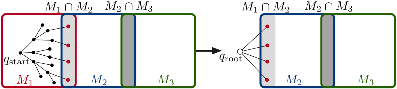
We propose the algorithm SMP^∗ that solves motion planning problems for a given sequence of manifolds. The algorithm searches for an optimal path that starts at an initial configuration, traverses the manifold sequence, and converges when the final manifold is reached. We solve this problem by growing a single tree over the manifold sequence. This tree consists of multiple subtrees that originate at the intersections between pairs of manifolds. We propose a novel steering strategy for RRT^∗ that guides the robot towards these manifold intersections. After an intersection is reached, a new subtree is initialized with the found intersection points and their costs. This approach allows us to use dynamic programming over optimal intersection points and scales well to long horizon tasks since a new subtree is initialized for every manifold. The algorithm is applicable to problems specified by a property regarding how the free configuration space changes across subtasks called intersection point independence (see Section IV).

A running example in this paper is the task of using a robot arm to transport a mug from one table to another while keeping the orientation of the mug upright. This task involves multiple phases and constraints that we describe informally as follows. First, the arm moves to pick up the mug. In this subtask, the arm can move freely in space and only needs to avoid collisions with obstacles. The second subtask is to grasp the mug. The third subtask is for the arm to transfer the mug with the goal keeping the mug upright at all times. The final subtask is to place and release the mug. This requires the base of the mug to be near the table for the gripper to successfully release the mug. We demonstrate our method in Section VI on similar tasks that involve multiple robots.

The main contributions of this work are a novel problem formulation for sequential motion planning on manifolds (Section IV), an algorithm to solve such problems for a certain class of planning problems (Section V), and proofs of probablistic completeness (Section VII) and asymptotic optimality (Section VIII) of the proposed algorithm. In Section VI, we demonstrate the performance of SMP^∗ on sequential kinematic planning problems and compare it to alternative planning strategies.

II Related Work

II-A Sampling-Based Motion Planning

Sampling-based motion planning (SBMP) is a randomized approach to path planning that builds a tree or graph in the robot configuration space. A PRM (probabilistic roadmap) is a path planner that builds a graph in the free configuration space that can be used for multiple queries [2, 22, 35]. Kavraki et al. [22] describe the method as a two-step procedure. First, a roadmap is built by sampling collision-free nodes and edges. Second, a path is found from a start to a goal state by using a graph search algorithm. This technique is multi-query, as it does not necessarily encode a specific start or end state, and thus can be reused for many planning problems with the same system. On the other hand, tree methods such as RRTs (rapidly-exploring random trees) are generally single-query, taking a specific start state from which a tree of feasible states is grown toward a goal state or region [31]. An advantage is that they can directly encode and respect kinodynamic and nonholonomic constraints. Many extensions to RRT exist, such as bidirectional trees and goal biasing [30, 32]. There also exist optimal variants RRT^∗ and PRM^∗, which find paths that minimize a cost function and guarantee asymptotic optimality by using a rewiring procedure [21]. All these techniques consider the problem of planning without motion constraints; that is, they plan in the free configuration space.

Here, we use a modified version of RRT^∗ in the inner loop of our algorithm that can handle goals defined in terms of equality constraints instead of a goal configuration. Restricting the problem class to intersection point independent problems (see Section IV-B) allows us to grow a single tree over a sequence of manifolds on which rewiring operations can still be performed. We show in Section VII and VIII that our algorithm inherits the probabilistic completeness and asymptotic optimality guarantees of RRT^∗.

II-B Constrained Sampling-Based Motion Planning

Planning with constraints is an important problem in robotics since it allows for the description of a wider range of tasks compared to the classical SBMP problem. An in-depth review of constrained SBMP can be found in Kingston et al. [25]. Constrained SBMP algorithms [45, 5, 17, 23, 26, 46, 11] extend SBMP to constrained configuration spaces, which are of smaller dimension than the full configuration space and usually cannot be sampled directly. An important aspect of these methods is how to generate samples and steer the robot while fulfilling the constraints.

One family of approaches are projection-based strategies [5, 45, 46] that first sample a configuration from the ambient configuration space and then project it using an iterative gradient descent strategy to a nearby configuration that satisfies the constraint. Kaiser et al. [20] considered the problem of finding a robot configuration that satisfies multiple constraints. They propose a solution where one constraint is set as the primary constraint on which a configuration is projected. Afterwards, the configuration is projected on remaining constraints while fulfilling the primary constraint. Berenson et al. [5] proposed the algorithm CBiRRT (constrained bidirectional RRT) that uses projections to find configurations that fulfill constraints. The constraints are described by task space regions, which are a representation of pose constraints. Their method can also be used for multiple constraints over a single path. However, their approach requires each constraint’s active domain to be defined prior to planning, or configurations are simply projected to the nearest manifold rather than respecting a sequential order. Our approach is perhaps closest to the CBiRRT algorithm. A main difference is that our method assumes a different problem formulation where the task is given in terms of a sequence of manifolds where the intersections between manifolds describe subgoals that the robot should reach. This problem formulation allows us to define a more structured steering strategy that guides the robot towards the next subgoals. Another difference is that CBiRRT does not search for optimal paths while we employ RRT^∗ to minimize the lengths of the path. We compare our method SMP^∗ to CBiRRT in the experimental section of this paper.

An alternative sampling strategy is to approximate the constraint surface by a set of local models and use this approximation throughout the planning problem for sampling or steering operations [17, 18, 23, 47, 45, 9]. AtlasRRT [18] builds an approximation of the constraint that consists of local charts defined in the tangent space of the manifold. This representation is used to generate samples that are close to the constraint. Similarly, Tangent Bundle RRT [23, 47] builds a bidirectional RRT by sampling a point on a tangent plane, extending this point to produce a new point, and if it exceeds a certain distance threshold from the center of the plane, projecting it on the manifold to create a new tangent plane. Bordalba et al. [9] addressed the problem of constrained kinodynamic planning by considering the fact that simulating ODEs will produce drift errors. They also propose an atlas-based method to address this problem by incorporating the creation of an atlas as the state space parameterization into the construction of a bidirectional RRT.

Kingston et al. [26] presented the implicit manifold configuration space (IMACS) framework that decouples two parts of a geometrically constrained motion planning problem: the motion planning algorithm and the method for constraint adherence. With this approach, IMACS acts as a representative layer between the configuration space and the planner that presents the constrained space to the planner. Many of the previously described techniques fit into this framework. They present examples with both projection-based and approximation-based methods for constraint adherence in combination with various motion planning algorithms.

In this work, we propose a method that builds on these constrained SBMP methods and extends them towards sequential tasks where the active constraints change during the motion.

II-C Sequential Motion Planning

One approach to plan sequential motions is task and motion planning (TAMP), which requires semantic reasoning on selecting and ordering actions to complete a higher-level task [19, 12, 29, 49, 13, 3, 10, 27, 36]. In general, TAMP is more difficult to solve due to scalability issues and the more complicated problem definition compared to SBMP. In our problem formulation, we assume that the sequence of tasks is given and focus on optimizing over the transition points between two constraints. Though we do not address task planning in this work, it is an interesting future direction we plan to consider.

Hauser and Ng-Thow-Hing [16] proposed the multi-modal motion planning algorithm Random-MMP, which plan motions over multiple mode switches that describe changes in the planning domain (e.g., contacts). Their planner builds a tree in a hybrid state that consists of the continuous robot configuration and a discrete mode. In each step of the algorithm, the tree is extended by randomly sampling mode switches and querying a SBMP to find a corresponding path. Informed expansion strategies like utility tables are used to incorporate prior knowledge of a task in order to improve the performance of the planner. Vega et al. [50] presented the Orbital Bellman trees (OBT) algorithm, which addresses the manipulation planning problem in a similar way. They introduce the notion of an orbit, which is the set of reachable configurations of a mode, and assume that they can sample configurations in an orbit as well as on its boundary. This functionality is used to generate random geometric graphs of configurations belonging to an orbit. During planning, such graphs are built for unexplored orbits and A^∗ is performed to connect the points of an orbit to its neighboring orbits. The paper also contains a factored variant that uses domain knowledge to reduce the number of graphs that need to be grown. Kingston et al. [27] proposed a similar multi-modal motion planning method. Instead of choosing random transitions between modes as in [16], they choose the transitions based on an informed search and the likelihood of a transition being successful, which is estimated online during the planning. Manipulation graphs are a similar framework to plan sequential manipulation tasks for robots [42]. The framework consists of graphs representing the continuous space of all feasible motions that the robot can perform, which are categorized into transit and transfer modes. A reduction property is defined that allows the graph to be represented by separate components that occur at the intersection of the two modes. Visibility-based PRMs [41] are used to represent the graphs and capture the closed-chain systems. Mirabel et al. [34] presented an algorithmic implementation of manipulation graphs for object manipulations where the constraints are also defined as level sets of equality constraints. They also present a graph builder that builds the constraint graph automatically. Schmitt et al. [39] extended this framework to also handle robot dynamics and time-variant environments.

Our work is similar to these approaches in that we also consider planning over multiple manifolds where changes in the configuration space occur due to picking or placing objects. In contrast to prior approaches, we do not assume that direct sampling of modes or switches is possible; rather, our algorithm is designed to find the mode-switching configurations during exploration toward manifold intersections. Further, we differ by specifying our problem formulation over a sequence of given manifolds and by applying this in the domain of intersection point independent problems, which we specify for sequential planning problems, and which are efficiently solvable by growing a single tree.

Trajectory optimization [51, 40, 48, 38, 7] is another approach to solve sequential motion planning problems. There, an optimization problem over a trajectory is defined that minimizes costs subject to constraints. This formulation is similar to our problem formulation in Equation (1) and allows us to describe complex behavior. However, trajectory optimization suffers from poor local minima and the need to specify costs and constraints activity for concrete time points. In complex tasks, it is difficult to specify how long a specific part of a motion takes in advance. Our approach only requires the sequential order of tasks and does not make any assumption of specific time points or durations of subtasks.

III Preliminaries

We begin with a brief background on differential geometry (see Boothby [8] for a rigorous treatment). An important idea in differential geometry is the concept of a manifold. A manifold is a surface which can be well-approximated locally using an open set of a Euclidean space. In general, manifolds are represented using a collection of local regions called charts and a continuous map associated with each chart such that the charts can be continuously deformed to an open subset of a Euclidean space. An alternate representation of manifolds, which is useful from a computational perspective, is to express them as zero level sets of functions defined on a Euclidean space. Such a representation of a manifold is called an implicit representation of the manifold. For example, a unit sphere embedded in $\mathbb{R}^{3}$ can be represented implicitly as $\{x\in\mathbb{R}^{3}~|~\|x\|-1=0\}$. An implicit manifold is said to be smooth if the implicit function associated with it is smooth. The set of all tangent vectors at a point on a manifold is a vector space called the tangent space of the manifold at that point. The null space of the Jacobian of the implicit function at a point is isomorphic to the tangent space of the corresponding manifold at that point. Since the tangent spaces of a manifold are vector spaces, we can equip them with an inner product structure which enables the computation of the length of curves traced on the manifold. A manifold endowed with an inner product structure is called a Riemannian manifold [33]. In this paper, we only consider smooth Riemannian manifolds.

IV Problem Formulation and Application Domain

We consider kinematic motion planning problems in a configuration space $C\subseteq\mathbb{R}^{k}$. A configuration $q\in C$ describes the state of one or multiple robots with $k$ degrees of freedom in total. We represent a manifold $M$ as an equality constraint $h_{M}(q)=0$ where

$$h_{M}(q):\mathbb{R}^{k}\to\mathbb{R}^{l}~.$$

The set of robot configurations that are on a manifold $M$ is given by

$$C_{M}=\{q\in C~|~h_{M}(q)=0\}~.$$

We define a projection operator

$$q_{\textrm{proj}}=\textit{Project}(q,M)$$

that takes a robot configuration $q\in C$ and a manifold $M$ as inputs and maps $q$ to a nearby configuration on the manifold $q_{\textrm{proj}}\in C_{M}$. We use an iterative optimization method, similar to [26, 5, 44], that iterates

$$q_{n+1}=q_{n}-J_{M}(q_{n})^{+}h_{M}(q_{n})$$

until a fixed point on the manifold is reached, which is checked by the condition $||h_{M}(q_{\textrm{proj}})||\leq\epsilon$. The matrix $J_{M}(q)^{+}$ is the pseudo-inverse of the constraint Jacobian

$$J_{M}(q)=\frac{\partial}{\partial q}h_{M}(q)~.$$

We are interested in solving tasks that are defined by a sequence of $n+1$ such manifolds

$$\mathcal{M}=\{M_{1},M_{2},\dots,M_{n+1}\}$$

and an initial configuration $q_{\textrm{start}}\in C_{M_{1}}$ that is on the first manifold. The goal is to find a path from $q_{\textrm{start}}$ that traverses the manifold sequence $\mathcal{M}$ and reaches a configuration on the goal manifold $M_{n+1}$. A path on the $i$-th manifold is defined as

$$\tau_{i}:[0,1]\to C_{M_{i}}$$

and $J(\tau_{i})$ is a cost function of a path

$${J}:\mathcal{T}\to\mathbb{R}_{\geq 0}$$

where $\mathcal{T}$ is the set of all non-trivial paths. We assume access to a collision check routine

$$\textit{CollisionFree}~:~C_{M}\times C_{M}\to\{0,1\}$$

that returns $1$ if the path between two configurations on the manifold is collision-free, $0$ otherwise. In the following problem formulation, we consider the scenario where the free configuration space $C_{\textrm{free}}$ changes during the task (e.g., when picking or placing objects). We define an operator $\Upsilon$ on the free configuration space $C_{\textrm{free}}$, which describes how $C_{\textrm{free}}$ changes as manifold intersections are traversed. $\Upsilon$ takes as input the path $\tau_{i-1}$ on the previous manifold $M_{i-1}$ and its associated $C_{\textrm{free}}$, which we denote as $C_{{\textrm{free}},i-1}$. $\Upsilon$ outputs an updated free configuration space

$$C_{{\textrm{free}},i}=\Upsilon(C_{{\textrm{free}},i-1},\tau_{i-1})$$

that accounts for the geometric changes due to transitioning to a new manifold.

Returning to our illustrative example, we can now describe one of its constraints more precisely. A simple grasp constraint can be described with $h_{M}(q)=x_{g}-f_{{\textrm{pos}},e}(q)$ where $f_{{\textrm{pos}},e}$ is the forward kinematics function of the robot end effector point $e$ and $x_{g}$ is the grasp location on the mug. This constraint can be fulfilled for multiple robot configurations $q$, which correspond to different hand orientations that will affect the free configuration space for the subsequent tasks. For example, if a mug was grasped from the side, it will have a different free space during the transport phase than if it was grasped from the top.

IV-A Problem Formulation

We formulate an optimization problem over a set of paths $\boldsymbol{\tau}=(\tau_{1},\dots,\tau_{n})$ that minimizes the sum of path costs under the constraints of traversing $\mathcal{M}$ and of being collision-free. The sequential manifold planning problem is

$$\begin{aligned} \boldsymbol{\tau}^{\star}=~&\underset{\boldsymbol{\tau}}{\operatorname{arg}\operatorname{min}}\;\sum_{i=1}^{n}J(\tau_{i})&&\\ {\textrm{s.t.}}\quad&\tau_{1}(0)=q_{\textrm{start}}&\\ &\tau_{i}(1)=\tau_{i+1}(0)&&\forall_{i=1,\dots,n-1}\\ &C_{{\textrm{free}},i+1}=\Upsilon(C_{{\textrm{free}},i},\tau_{i})~~~~&&\forall_{i=1,\dots,n}\\ &\tau_{i}(s)\in C_{M_{i}}\cap C_{{\textrm{free}},i}&&\forall_{i=1,\dots,n}~\forall_{s\in[0,1]}\\ &\tau_{n}(1)\in C_{M_{n+1}}\cap C_{{\textrm{free}},n+1}&&\end{aligned}$$ (1)

The second constraint ensures continuity such that the endpoint of a path $\tau_{i}(1)$ is the start point of the next path $\tau_{i+1}(0)$. The third constraint captures the change in the collision-free space defined by the operator $\Upsilon$. The last two constraints ensure that the path is collision free and on the corresponding manifolds. The endpoint of $\tau_{n}$ must be on the goal manifold $M_{n+1}$, which denotes the successful completion of the task.

An advantage of this formulation is that it is not necessary to specify a target configuration in $C$. A wider range of goals (e.g., in the robot end effector space) can be described in the form of manifolds. Another advantage is that it is possible to describe complex sequential tasks in a single planning problem, not requiring the specification of subgoal configurations. The algorithm that is proposed in Section V searches for a path that solves this optimization problem for the problem class described in the next section.

Fig. 2: Initialization of a new subtree (steps 30–33 of Algorithm 1). The reached goal nodes at the intersection $M_{1}\cap M_{2}$ are used to initialize the next tree where $q_{\textrm{root}}$ is a synthetic root node that ensures the tree structure.

IV-B Intersection Point Independent Problems

We now use the problem formulation in (1) to describe robotic manipulation planning problems in which the manifolds describe subtasks that the robot needs to complete (e.g., picking up objects). The solution is an end-to-end path across multiple task constraints. In manipulation tasks, it is common that the geometry changes throughout the motion due to picking up or placing objects. Here, we make the assumption that these changes only occur at the transition between two manifolds. For example, changing the grasp of a mug will only occur at points during the task when it is picked up or placed.

For a certain class of sequential manifold planning problems, the following property holds: For each manifold intersection ${M}_{i}\cap{M}_{i+1}$, the free space output by $\Upsilon$ is set-equivalent for every possible path $\tau_{i}$. In other words, the precise action taken to move the configuration from one constraint to the next does not affect the feasible planning space for the subsequent subtask. When this property holds for all intersections, we call the problem intersection point independent. The condition for this class of problems is

$$\begin{aligned} &\forall i\in[0,n]~\forall\tau_{i},\tau_{i}^{\prime}\in\mathcal{T}:\tau(1),\tau^{\prime}(1)\in C_{M_{i}}\cap C_{M_{i+1}}\\ &\Rightarrow\Upsilon(C_{{\textrm{free}},i},\tau)\equiv\Upsilon(C_{{\textrm{free}},i},\tau^{\prime})\end{aligned}$$ (2)

where $\equiv$ denotes set-equivalence. In this work, we focus on the intersection point independent class of motion planning problems, which encompass a wide range of common problems. For grasping constraints, a notion of object symmetry about the grasp locations results in intersection point independent problems. If the object to be grasped is a cylindrical can, for example, allowing grasps to occur at any point around the circumference but at a fixed height would be intersection point independent. Any two grasps with the same relative orientation of the gripper result in the same free configuration space of the system (robot + can). However, suppose the grasps can occur at any height on the can. Now, a grasp near the top of the can and a grasp in the middle of the can result in different free configuration spaces, and thus this would be an intersection point dependent problem.

Focusing on intersection point independent problems allows us to define an efficient algorithm that grows a single tree over a sequence of manifolds. The more general intersection point dependent problems covers a wider descriptions of problems. However, they are more difficult to solve because they require the handling of foliated manifolds [24] (e.g., every grasp leads to a different manifold). Our illustrative example is one such problem, since the grasp on the handle and the grasp from the top of the mug result in different free spaces. We plan to address this more complex problem class in future work and provide some insights in Section IX how the proposed algorithm could be used to tackle them.

V Sequential Manifold Planning

In this section, we present the algorithm SMP^∗ that solves the problem formulated in Equation (1). The algorithm searches for an optimal solution to the constrained optimization problem, which is a sequence of paths $\boldsymbol{\tau}=(\tau_{1},\dots,\tau_{n})$ where each $\tau_{i}$ is a collision-free path on the corresponding manifold $M_{i}$. The steps of SMP^∗ are outlined in Algorithm 1. The input to the algorithm is a sequence of manifolds $\mathcal{M}$ and an initial configuration $q_{\textrm{start}}\in M_{1}$ on the first manifold.

The overall problem is divided into $n$ subproblems. In each subproblem, a tree is grown from a set of initial nodes towards the intersection of the current and next manifold $M_{i}\cap M_{i+1}$. In the inner loop of the algorithm (lines 4–24), the steps are similar to RRT^∗ and the rewiring step in the RRT^∗_EXTEND routine (Algorithm 2) is equivalent to the one in RRT^∗ [21]. The extend operation uses a distance function $c(q_{0},q_{1})\in\mathbb{R}_{\geq 0}$ between two nearby configurations and a function Cost$(q)$ that stores the path costs from the root of the tree to a node $q$. The main modifications with respect to RRT^∗ are in the extension and projection steps. Instead of targeting a single goal configuration as done in general SBMP, we propose two novel steering strategies that steer towards the intersection between manifolds $M_{i}\cap M_{i+1}$.

In steps 5–12, a new target point $q_{\textrm{rand}}$ in the configuration space is sampled and its nearest neighbor $q_{\textrm{near}}$ in the tree is computed. Next, one of the following two steering strategies is selected to find a direction $d$ in which to extend the tree.

1. ${\textrm{{SteerPoint}}}(q_{0},q_{1},M_{i})$ extends the tree from $q_{0}\in C_{M_{i}}$ towards $q_{1}\in C$ while staying on the current manifold $M_{i}$.

2. ${\textrm{{SteerConstraint}}}(q_{0},M_{i},M_{i+1})$ extends the tree from $q_{0}\in C_{M_{i}}$ towards the intersection of the current and next manifold $M_{i}\cap M_{i+1}$.

Both steering steps are described in detail in Section V-A and V-B. Similar to the goal bias in RRT, a parameter $\beta\in[0,1]$ specifies the probability of selecting the SteerConstraint step. Then, a new point $q_{\textrm{new}}$ is computed by taking a step in direction $d$ from $q_{\textrm{near}}$ with the maximum step size $\alpha\in\mathbb{R}_{>0}$. Before the point is added to the tree, it is projected onto a manifold (steps 13–17). Depending on the distance to the intersection of the manifolds, which is measured with $||h_{M_{i+1}}(q_{\textrm{new}})||$, the point is projected either on the manifold $M_{i}$ or on the intersection manifold $M_{i}\cap M_{i+1}$. The threshold for this condition is sampled uniformly between $0$ and $r_{\textrm{max}}$, where the parameter $r_{\textrm{max}}\in\mathbb{R}_{>0}$ describes the closeness required by a point around $M_{i+1}$ to be projected onto $M_{i}\cap M_{i+1}$. This randomization is necessary in order to achieve probabilistic completeness that is shown in Section VII, which also gives a formal definition of $r_{\textrm{max}}$. Afterward, the RRT^∗_EXTEND routine described in Algorithm 2 is called with the projected $q_{\textrm{new}}$ point. This routine checks the point for collision with the current free configuration space $C_{{\textrm{free}},i}$, performs rewiring steps, and eventually adds the point to the tree. The point is also added to a set of goal nodes $V_{\textrm{goal}}$ if it is on the intersection manifold $M_{i}\cap M_{i+1}$. In order to avoid duplicate intersection nodes, we ensure a minimum distance $\rho\in\mathbb{R}_{>0}$ between two nodes in $V_{\textrm{goal}}$ (step 20). After each time the inner loop of SMP^∗ is completed, a new tree is initialized in steps 30–33 with all the intersection nodes in $V_{\textrm{goal}}$ and their costs so far. In order to keep the tree structure, we add a synthetic root node $q_{\textrm{root}}$ as parent node for all intersection nodes (see Figure 2). Convergence of the algorithm can be defined in various ways. We typically set an upper limit to the number of intersection nodes or provide a time limit for the inner loop. After reaching the last manifold, the algorithm returns the path with the lowest cost that reached the goal manifold $M_{n+1}$.

In the following sections, the steering strategies SteerPoint and SteerConstraint are derived.

1: $V_{1}=\{q_{{\textrm{start}}}\}$; $E_{1}=\emptyset$

2: for i=1 to n do

3:   $V_{\textrm{goal}}=\emptyset$

4:   while TimeRemaining() do

5:    $q_{\textrm{rand}}\leftarrow{\textrm{Sample}}(C)$

6:    $q_{\textrm{near}}\leftarrow{\textrm{Nearest}}(V_{i},q_{\textrm{rand}})$

7:    if $\mathcal{U}(0,1)<\beta$ then

8:      $d\leftarrow{\textrm{SteerConstraint}}(q_{\textrm{near}},M_{i},M_{i+1})$

9:    else

10:      $d\leftarrow{\textrm{SteerPoint}}(q_{\textrm{near}},q_{\textrm{rand}},M_{i})$

11:    end if

12:    $q_{\textrm{new}}\leftarrow q_{\textrm{near}}+\alpha\frac{d}{||d||}$

13:    if $||h_{M_{i+1}}(q_{\textrm{new}})||<\mathcal{U}(0,r_{\textrm{max}})$ then

14:      $q_{\textrm{new}}\leftarrow{\textrm{Project}}(q_{\textrm{new}},M_{i}\cap M_{i+1})$

15:    else

16:      $q_{\textrm{new}}\leftarrow{\textrm{Project}}(q_{\textrm{new}},M_{i})$

17:    end if

18:    if RRT^∗_EXTEND$(V_{i},E_{i},q_{\textrm{near}},q_{\textrm{new}})$ then

19:      if $||h_{M_{i+1}}(q_{\textrm{new}})||<\epsilon$ and

20: $\hskip 55.00008pt||{\textrm{Nearest}}(V_{\textrm{goal}},q_{\textrm{new}})-q_{\textrm{new}}||\geq\rho$ then

21:       $V_{\textrm{goal}}\leftarrow V_{\textrm{goal}}\cup q_{\textrm{new}}$

22:      end if

23:    end if

24:   end while

25:   // return path with lowest costs when $M_{n+1}$ is reached

26:   if $i=n$ then

27:    return $\mathrm{OptimalPath}(V_{1:n},E_{1:n},q_{\textrm{start}},M_{n+1})$

28:   end if

29:   // initialize next tree with the intersection nodes

30:   $q_{\textrm{root}}={\textrm{null}},V_{i+1}=\{q_{\textrm{root}}\};E_{i+1}=\emptyset$

31:   for $q\in V_{\textrm{goal}}$ do

32:    $V_{i+1}\leftarrow V_{i+1}\cup\{q\};E_{i+1}\leftarrow E_{i+1}\cup\{(q_{\textrm{root}},q)\}$

33:   end for

34: end for

Algorithm 1 SMP^∗ $(\mathcal{M},q_{{\textrm{start}}},\alpha,\epsilon,\rho,r_{\textrm{max}})$

1: if ${\textrm{CollisionFree}}(q_{\textrm{near}},q_{\textrm{new}})$ then

2:  $Q_{\textrm{near}}={\textrm{Near}}\Big(V,q_{\textrm{new}},\underset{}{\operatorname{min}}\;\Big\{\gamma_{\textrm{RRT*}}\left(\tfrac{\log(|V|)}{|V|}\right)^{1/k}\!,\alpha\Big\}\Big)$

3:  $V\leftarrow V\cup\{q_{{\textrm{new}}}\}$

4:  $q_{\textrm{min}}=q_{\textrm{near}}$; $c_{\textrm{min}}={\textrm{Cost}}(q_{\textrm{near}})+c(q_{\textrm{near}},q_{\textrm{new}})$

5:  for $q_{\textrm{near}}\in Q_{\textrm{near}}$ do

6:   if ${\textrm{CollisionFree}}(q_{\textrm{near}},q_{\textrm{new}})$ and

7: $\quad\qquad{\textrm{Cost}}(q_{\textrm{near}})+c(q_{\textrm{near}},q_{\textrm{new}})<c_{\textrm{min}}$ then

8:    $q_{\textrm{min}}=q_{\textrm{near}}$; $c_{\textrm{min}}={\textrm{Cost}}(q_{\textrm{near}})+c(q_{\textrm{near}},q_{\textrm{new}})$

9:   end if

10:  end for

11:  $E\leftarrow E\cup\{(q_{\textrm{min}},q_{\textrm{new}})\}$

12:  for $q_{\textrm{near}}\in Q_{\textrm{near}}$ do

13:   if ${\textrm{CollisionFree}}(q_{\textrm{new}},q_{\textrm{near}})$ and

14: $\qquad\quad{\textrm{Cost}}(q_{\textrm{new}})+c(q_{\textrm{new}},q_{\textrm{near}})<{\textrm{Cost}}(q_{\textrm{near}})$ then

15:    $q_{\textrm{parent}}={\textrm{Parent}}(q_{\textrm{near}})$

16:    $E\leftarrow E~\backslash~\{(q_{\textrm{parent}},q_{\textrm{near}})\}$

17:    $E\leftarrow E\cup\{(q_{\textrm{new}},q_{\textrm{near}})\}$

18:   end if

19:  end for

20:  return True

21: else

22:  return False

23: end if

Algorithm 2 RRT^∗_EXTEND$~(V,E,q_{\textrm{near}},q_{\textrm{new}})$

V-A ${\textrm{SteerPoint}}(q_{0},q_{1},M_{i})$

In this extension step, the robot is at $q_{0}\in C_{M_{i}}$ and should step towards the target configuration $q_{1}\in C$ while staying on the manifold $M_{i}$. We formulate this problem as a constrained optimization problem of finding a curve $\gamma~:~[0,1]\to C$ that

$$\begin{aligned} &\underset{\gamma}{{\textrm{minimize}}}\;&&||\gamma(1)-q_{1}||^{2}\\ &{\textrm{subject to}}~~&&\gamma(0)=q_{0}\\ &&&\int_{0}^{1}||\dot{\gamma}(t)||~\mathrm{d}s\leq\alpha\\ &&&h_{M_{i}}(\gamma(s))=0\quad\qquad\forall~s\in[0,1]\end{aligned}$$ (3)

This problem is hard to solve due to the nonlinear constraints. Since the steering operations are called many times in the inner loop of the algorithm, we choose a simple curve representation and only compute an approximate solution to this problem. We parameterize the curve as a straight line with length $\alpha$.

$$\gamma(s)=q_{0}+s\alpha\frac{d}{||d||}$$ (4)

Further, we apply a first-order Taylor expansion of the manifold constraint $h_{M_{i}}(q_{0}+d)\approx h(q_{0})+J_{M_{i}}(q_{0})d~.$ The problem is reduced to finding a direction $d$ that

$$\begin{aligned} &\underset{d}{{\textrm{minimize}}}\;&&\frac{1}{2}||d-(q_{1}-q_{0})||^{2}\\ &{\textrm{subject to}}~~&&J_{M_{i}}(q_{0})d=0\end{aligned}$$ (5)

which has the optimal solution

$$\begin{aligned} d&=(I-J_{M_{i}}^{\top}(J_{M_{i}}J_{M_{i}}^{\top})^{-1}J_{M_{i}})(q_{1}-q_{0})\\ &=V_{\bot}V_{\bot}^{\top}(q_{1}-q_{0})\end{aligned}$$ (6)

where $V_{\bot}$ contains the singular vectors that span the right nullspace of $J_{M_{i}}$ [37]. We normalize $d$ later in the algorithm, and thus do not include the constraint $||d||\leq\alpha$ in the reduced optimization problem. The new configuration $q_{0}+\alpha\frac{d}{||d||}$ will be on the tangent space of the manifold at configuration $q_{0}$, so that only few projection steps will be necessary before it can be added to the tree.

V-B ${\textrm{SteerConstraint}}(q_{0},M_{i},M_{i+1})$

This steering step extends the tree from $q_{0}\in C_{M_{i}}$ towards the intersection of the current and next manifold $M_{i}\cap M_{i+1}$, which can be expressed as the optimization problem

$$\begin{aligned} &\underset{\gamma}{{\textrm{minimize}}}\;&&||h_{M_{i+1}}(\gamma(1))||^{2}\\ &{\textrm{subject to}}\quad&&\gamma(0)=q_{0}\\ &&&\int_{0}^{1}||\dot{\gamma}(t)||~\mathrm{d}s\leq\alpha\\ &&&h_{M_{i}}(\gamma(s))=0\quad\qquad\forall~s\in[0,1]\end{aligned}$$ (7)

The difference from problem (3) is that the loss is now specified in terms of the distance to the next manifold $h_{M_{i+1}}(\gamma(1))$. This cost pulls the robot towards the manifold intersection. Again, we approximate the curve with a line (Equation (4)) and apply a first-order Taylor expansion to the nonlinear terms, which results in the simplified problem

$$\begin{aligned} &\underset{d}{{\textrm{minimize}}}\;&&\frac{1}{2}||h_{M_{i+1}}(q_{0})+J_{M_{i+1}}(q_{0})d||^{2}\\ &{\textrm{subject to}}~~&&J_{M_{i}}(q_{0})d=0~.\end{aligned}$$ (8)

A solution $d$ can be obtained by solving the linear system

$${\scriptscriptstyle{\left(\hskip-2.15277pt\begin{array}[]{c c}J_{M_{i+1}}^{\top}J_{M_{i+1}}&J_{M_{i+1}}^{\top}\\ J_{M_{i}}&0\end{array}\hskip-2.15277pt\right)}}{\scriptscriptstyle{\left(\hskip-2.15277pt\begin{array}[]{c}d\\ \lambda\end{array}\hskip-2.15277pt\right)}}={\scriptscriptstyle{\left(\hskip-2.15277pt\begin{array}[]{c}-J_{M_{i+1}}^{\top}h_{M_{i+1}}\\ 0\end{array}\hskip-2.15277pt\right)}}$$

where $\lambda$ are the Lagrange variables. The solution is in the same direction as the steepest descent direction of the loss projected onto the tangent space of the current manifold.

A reference implementation of this algorithm in Python is made available on GitHub .

VI Evaluation

In the following experiments, we solve kinematic motion planning problems where the cost function measures path length. We compare the proposed method SMP^∗ (Algorithm 1) with three alternative methods:

• Greedy SMP^∗ – Algorithm 1 with the modification that only the node with the lowest cost in $V_{\textrm{goal}}$ is selected to initialize the next tree (steps 30 – 33 of Algorithm 1).

• RRT^∗+IK – This is a two-step procedure. First, a point on the manifold intersection is generated via inverse kinematics by randomly sampling a point in $C$ and projecting it onto the manifold intersection. Next, RRT^∗ is applied to compute a path towards this node. This procedure is repeated until the goal manifold is reached.

• CBiRRT – The Constrained Bidirectional Rapidly-Exploring Random Tree algorithm [4, 5] grows two trees towards each other with the RRT Connect strategy [30]. In each steering step, the sampled configuration is projected onto the manifold with the lowest level set function value.

We executed all methods with the same upper time limit and compared the quality of found paths in terms of the given objective.

VI-A 3D Point on Geometric Constraints

We demonstrate the performance of the proposed algorithm on a 3D point that needs to traverse three constraints defined by geometric primitives. The initial robot state is $q_{\textrm{start}}=(3.5,3.5,4.45)$ and the sequence of manifolds is

1. Paraboloid:

   $${M_{1}}(q)=0.1q_{1}^{2}+0.1q_{2}^{2}+2-q_{3}$$

2. Cylinder:

   $$h_{M_{2}}(q)=0.25q_{1}^{2}+0.25q_{2}^{2}-1.0$$

3. Paraboloid:

   $$h_{M_{3}}(q)=-0.1q_{1}^{2}-0.1q_{2}^{2}-2-q_{3}$$

4. Goal point:

   $$h_{M_{4}}(q)=q-q_{\textrm{goal}}$$

   with the goal configuration $q_{\textrm{goal}}=(-3.5,-3.5,-4.45)$.

We evaluate the algorithms on two variants of this problem. An obstacle-free variant (visualized in Figure 1) and a variant that contains four box obstacles placed at the intersections between the manifolds (visualized in Figure 3). The configuration space is limited to $[-6,6]$ in all three dimensions and the time limit for growing a tree is 10 s for all methods. Note that CBiRRT does not optimize an objective function and immediately converges when it finds a feasible path, which achieves an overall lower computation time. In this experiment, the computation time of CBiRRT was $2.45\pm 0.44$ s. The parameters of the algorithms are $\alpha=1.5$, $\beta=0.05$, $\epsilon=0.01$, $\rho=0.1$, and $r_{\textrm{max}}=1.5$. In Figure 1, $q_{\textrm{start}}$ is drawn as red point and $q_{\textrm{goal}}$ as blue point. The intersection nodes $V_{\textrm{goal}}$ are shown as magenta points and a solution path from SMP^∗ is visualized as a line. Figure 3 shows a set of found paths on the variant with obstacles. Only SMP^∗ is able to find the optimal intersection regions between the obstacles. The path costs of the four algorithms are summarized in the table in Figure 4. The results show that SMP^∗ finds the path with the lowest cost. CBiRRT and RRT^∗+IK do not optimize over the intersection points, which explains the higher costs and standard deviations. Greedy SMP^∗ always selects the best intersection point, which improves the path costs compared to CBiRRT and RRT^∗+IK. However, these greedily selected intersection points are not necessarily the best choice for the global path. SMP^∗ searches over the intersection points in a more profound manner and selects the optimal sequence of explored intersection points for the final path.

Fig. 3: Samples of found paths on the geometric constraints w/ obstacles problem (Section VI-A).

	w/o obstacles	w/ obstacles
SMP∗	$14.36\pm 0.02$	$15.54\pm 0.09$
Greedy SMP∗	$16.15\pm 0.03$	$21.31\pm 0.70$
CBiRRT	$17.04\pm 2.65$	$20.29\pm 3.04$
RRT∗+IK	$17.56\pm 2.33$	$20.89\pm 4.51$

Fig. 4: Path costs of the 3D point on geometric constraints experiment. We report the mean and one unit standard deviation over 50 runs.

(a)

(b)

Fig. 5: Path costs over variations of the parameter $\rho$ (left) and over the phase of the motion $s$ (right) on the geometric constraints w/o obstacles problem (Section VI-A). The graphs show the mean and unit standard deviation over $50$ trials. In (a), the costs are increasing for higher values of $\rho$. For larger values, the performance of SMP^∗ is very similar to the Greedy SMP^∗ strategy. In (b), Greedy SMP^∗ finds shorter paths to the first two manifold intersections while the overall best solutions towards the target manifold is found by SMP^∗.

In Figure 5a, the path costs $J(\tau)$ of SMP^∗ and Greedy SMP^∗ are compared for various values of the parameter $\rho$. This parameter specifies the minimum distance between two intersection points, which influences the number of intersection points created during planning (step 20 in Algorithm 1). The results show that the found paths of SMP^∗ with a lower $\rho$ lead to lower costs. For larger $\rho$, the performance of SMP^∗ converges to the same performance as Greedy SMP^∗ since only a single intersection point is considered.

Figure 5b visualizes the cost over the phase of the path where $s\in[0,1]$ parameterizes the path on the first manifold $M_{1}$, $s\in[1,2]$ on $M_{2}$ and $s\in[2,3]$ on $M_{3}$. The results indicate that the Greedy SMP^∗ strategy finds paths that reach the intersections of $M_{1}\cap M_{2}$ and $M_{2}\cap M_{3}$ with lower costs. However, SMP^∗ finds the path that achieves the overall task of reaching the goal manifold $M_{4}$ with the lowest mean cost and standard deviation where it outperforms RRT^∗+IK and CBiRRT.

VI-B Multi-Robot Object Transport Tasks

(a) Task A

(b) Task B

(c) Task C

Fig. 6: Object transport tasks where the goal is to transport the red and blue object to the green target locations.

Fig. 7: Snapshots of the resulting motion that SMP^∗ found for Task C.

	Task A	Task B	Task C
SMP∗	$7.94\pm 0.69$	$13.58\pm 1.14$	$27.07\pm 2.58$
RRT∗+IK	$9.46\pm 1.65$	–	–
Greedy SMP∗	$8.56\pm 1.24$	$14.22\pm 1.71$	$31.75\pm 2.51$

Fig. 8: Results of object transport experiment. We report the mean and one unit standard deviation over 10 runs.

In this experiment, we demonstrate SMP^∗ on various object transportation tasks. The overall task objective is to transport an object from an initial to a goal location. We consider three variations of this task:

• Task A: A single robot arm mounted on a table with $k=6$ degrees of freedom. The task is to transport an object from an initial location on the table to a target location. This task is described by $n=3$ manifolds.

• Task B: This task consists of two robot arms and a mobile base consisting of $k=14$ degrees of freedom. The task is defined such that the first robot arm picks the object and places it on the mobile base. Then, the mobile base brings it to the second robot arm that picks it up and places it on the table. This procedure is described with $n=5$ manifolds.

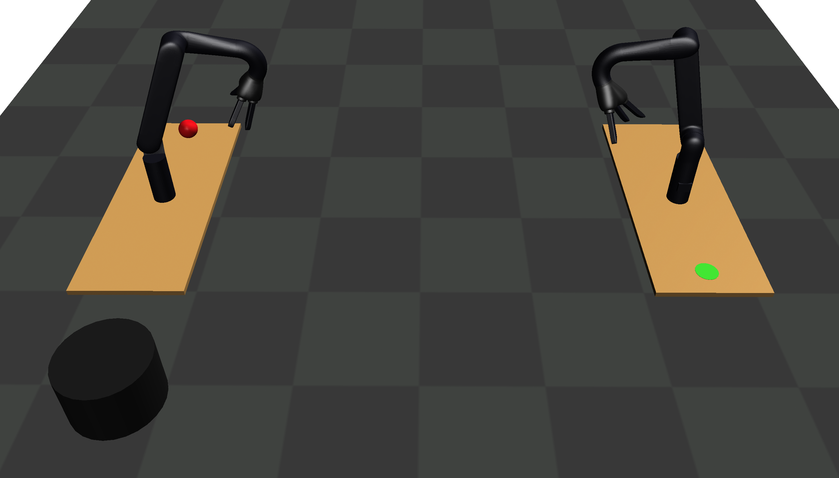
• Task C: In this task, four robots are used that need to transport two objects between two tables. Three arms are mounted on the tables and another arm with a tray is mounted on a mobile base. Besides transporting the objects, the orientation of the two objects needs to be kept upright during the whole motion. This task is described with $n=12$ manifolds and the configuration space has $k=26$ degrees of freedom.

The three tasks are visualized in Figure 6 where the target locations are shown as green areas. The geometries of the objects were chosen such that the tasks fall into the intersection point independent category (see Section IV-B). Three types of constraints are used to describe these tasks. Picking up an object is defined with the constraint $h_{M}(q)=x_{g}-f_{{\textrm{pos}},e}(q)$ where $x_{g}\in\mathbb{R}^{3}$ is the location of the object and $f_{{\textrm{pos}},e}(q)$ is the forward kinematics function to a point $e\in\mathbb{R}^{3}$ on the robot end effector. The handover of an object between two robots is described by $h_{M}(q)=f_{{\textrm{pos}},e_{1}}(q)-f_{{\textrm{pos}},e_{2}}(q)$ where $f_{{\textrm{pos}},e_{1}}(q)$ is the forward kinematics function to the end effector of the first robot and $f_{{\textrm{pos}},e_{2}}(q)$ is that of the second robot. The orientation constraint is given by an alignment constraint $h_{M}(q)=f_{{\textrm{rot}},z}(q)^{\top}e_{z}-1$ where $f_{{\textrm{rot}},z}(q)$ is a unit vector attached to the robot end effector that should be aligned with the vector $e_{z}=(0,0,1)$ to point upwards. These constraints are sufficient to describe the multi-robot transportation tasks. The parameters of the algorithms are $\alpha=0.5$, $\beta=0.2$, $\epsilon=1e-5$, $\rho=0.1$, and $r_{\textrm{max}}=0.5$. The time limit for all strategies is 60 s.

The costs of the SMP^∗, Greedy SMP^∗ and RRT^∗+IK algorithms are reported in Figure 8. SMP^∗ outperforms the other algorithms on all tasks. The RRT^∗+IK strategy was not able to solve Tasks B or C. A found solution of SMP^∗ for Task C is visualized in Figure 7. The resulting motions of all tasks are also shown in a supplementary video.

VII Probabilistic Completeness

In this section, we prove the probabilistic completeness of our algorithm. Note that for ease of analysis, the analysis presented in this section and in the subsequent section assumes that $\rho=0$ in Algorithm 1. In the future, we will analyze the properties of our approach when $\rho$ is strictly positive. Moreover, in this analysis we refer to the collision free region of a manifold when we allude to $M_{i}$.

Definition 1

A collision-free path is said to have strong $\delta$-clearance if the path lies entirely inside the $\delta$-interior of $\cup\mathcal{M}$, where $\cup\mathcal{M}\triangleq\cup_{i=1}^{n+1}M_{i}$.

We start by assuming that there exists a path $\hat{\boldsymbol{\tau}}$ with strong $\delta$-clearance connecting the goal manifold $M_{n+1}$ with the start configuration $q_{\textrm{start}}$ embedded on the sequence of manifolds under consideration. Let $L$ be the total length of the path, computed based on the pullback metric [33] of the manifolds due to their embedding in $\mathbb{R}^{k}$. Let $\xi>0$ be the minimum over the reach [1] of all manifolds in the sequence and the manifolds resulting from the pairwise intersection of adjacent manifolds in the sequence. Informally, the reach of a manifold is the size of an envelope around the manifold such that any point within the envelope and the manifold has an unique projection onto the manifold. For the analysis presented here, we pick the steering parameter $\alpha$ such that $\xi\geq\alpha$. We use the notation $\textit{Tube}(M_{i},\xi)$ to denote the set $\{x\in\mathbb{R}^{k}~|~d(x,M_{i})<\xi\}$, where

$$d(x,M_{i})=\inf\{\|x-y\|_{\mathbb{R}^{k}}|\ y\in M_{i}\}$$ (15)

is the minimum distance of the point $x$ to the manifold. Now, if we define

$$\zeta_{i}=\sup\limits_{q\in\textit{Tube}(M_{i},\xi)}\|h_{M_{i}}(q)\|,$$ (16)

then for the sake of analysis we assume that $r_{\textrm{max}}=\underset{\ }{\operatorname{max}}\;\{\zeta_{1},\cdots,\zeta_{n+1}\}$. If $\nu=\underset{\ }{\operatorname{min}}\;(\delta,\alpha)$, then we define a sequence of points

$$\{ [q^{1}_{0}=q_{\textrm{start}},q^{1}_{1},\cdots,q^{1}_{m_{1}}],[q^{2}_{0},q^{2}_{1},\cdots,q^{2}_{m_{2}}],\cdots,$$

$$[q^{n}_{0},q^{n}_{1},\cdots,q^{n}_{m_{1}}],[q^{n+1}_{0}]\}$$ (17)

on $\hat{\boldsymbol{\tau}}$, such that $[q^{i}_{0},q^{i}_{1},\cdots,q^{i}_{m_{i}}]\in M_{i}$ and $\sum_{i=1}^{n}m_{i}=m$, where $m=\frac{5L}{\nu(n+1)}$ is the total number of points in the path. Without loss of generality, we assume that for every $M_{i}$ with $1<i<n+1$ there exists a non-negative integer $j<m_{i}$ such that $q^{i}_{0},q^{i}_{1},\cdots,q^{i}_{j}\in M_{i-1}\cap M_{i}$ and $q^{i}_{j+1},q^{i}_{j+2},\cdots,q^{i}_{m_{i}}\in M_{i}\setminus M_{i+1}$. In other words, there exist some points at the beginning of $[q^{i}_{0},q^{i}_{1},\cdots,q^{i}_{m_{i}}]$ that belong to $M_{i-1}\cap M_{i}$ and the rest of the points on the manifold belong exclusively to $M_{i}$. For ease of analysis, the sequence of points on $\hat{\boldsymbol{\tau}}$ is chosen such that

$$\|q^{i}_{j}-q^{i}_{j+1}\|_{M_{i}}\leq\|q^{i}_{j}-q^{i}_{j+1}\|_{\mathbb{R}^{k}}\leq\nu/5,$$ (18)

where $\|\cdot\|_{M_{i}}$ and $\|\cdot\|_{\mathbb{R}^{k}}$ are the distances between the points according to the metrics on the manifold and ambient space respectively. We use $B(q^{i}_{j},\nu)\subset\mathbb{R}^{k}$ to denote a ball of radius $\nu$ around $q^{i}_{j}$ under the standard Euclidean norm on $\mathbb{R}^{k}$. We denote the tree that is grown with RRT^∗ as $T$.

We prove the probabilistic completeness of our strategy in two parts. The first part proves the probabilistic completeness of RRT^∗ on a single manifold. In the second part, we prove that with probability one, the tree $T$ grown on a manifold can be expanded onto the next manifold as the number of samples tends to infinity. For the first part, as suggested in [26, Section 5.3], the Lemma 1 in [28] can be shown to hold for the single manifold case and probabilistic completeness of RRT/RRT^∗ on a manifold can be easily proven using [28, Theorem 1]. We now focus on proving the second part that shows the probabilistic completeness of our strategy. We start by proving Lemma 1 which enables us to prove that a tree grown with RRT^∗ on a manifold can be extended to the next manifold.

Lemma 1

Suppose that ${T}$ has reached $M_{i}$ and contains a vertex $\tilde{q}^{i}_{m_{i}}$ such that $\tilde{q}^{i}_{m_{i}}\in B(q^{i}_{m_{i}},\nu/5)$. If a random sample $q_{\textrm{rand}}^{i+1}$ is drawn such that $q_{\textrm{rand}}^{i+1}\in B(q^{i+1}_{0},\nu/5)$, then the straight path between $\textit{Project}(q_{\textrm{rand}}^{i+1},M_{i}\cap M_{i+1})$ and the nearest neighbor $q_{\textrm{near}}$ of $q_{\textrm{rand}}^{i+1}$ in $T$ lies entirely in $C_{{\textrm{free}},i+1}$.

Proof:

By definition $\|q_{\textrm{near}}-q_{\textrm{rand}}^{i+1}\|\leq\|\tilde{q}^{i}_{m_{i}}-q_{\textrm{rand}}^{i+1}\|$, then using the triangle inequality and some algebraic manipulation similar to that used in the proof of [28, Lemma 1], we can show that

$$\|q_{\textrm{near}}-q^{i}_{m_{i}}\|~\leq~ \|\tilde{q}^{i}_{m_{i}}-q^{i}_{m_{i}}\|+2\|x^{i+1}_{0}-q_{\textrm{rand}}^{i+1}\|$$

$$+2\|q^{i}_{m_{i}}-q^{i+1}_{0}\|$$ (19)

which leads to $\|q_{\textrm{near}}-q^{i}_{m_{i}}\|\leq 5\frac{\nu}{5}\leq\nu$ and $q_{\textrm{near}}\in B(q^{i}_{m_{i}},\nu)$. Again, by the triangle inequality, we can show that $\|q_{\textrm{near}}-q_{\textrm{rand}}^{i+1}\|\leq\nu$. As the sample $q_{\textrm{rand}}^{i+1}$ is taken from within the reach of $M_{i}$ there exists a unique nearest point of $q_{\textrm{rand}}^{i+1}$ on $M_{i}$ [1]. In other words, the operation $\textit{Project}(q_{\textrm{rand}}^{i+1},M_{i}\cap M_{i+1})$ is well-defined. Therefore, as

$$\|q_{\textrm{near}}-\textit{Project}(q_{\textrm{rand}}^{i+1},M_{i}\cap M_{i+1})\|\leq\|q_{\textrm{near}}-q_{\textrm{rand}}^{i+1}\|\leq\nu,$$ (20)

the straight path between $\textit{Project}(q_{\textrm{rand}}^{i+1},M_{i}\cap M_{i+1})$ and $q_{\textrm{near}}$ lies entirely in $C_{{\textrm{free}},i+1}$. ∎

Note that the above lemma is an extension of [28, Lemma 1]. The next theorem will prove that with probability one SMP^∗ will yield a path as the number of samples goes to infinity. Since we are only concerned about the transition of $T$ from one manifold to the next, we focus on the iterations in SMP^∗ after $T$ reaches a neighborhood of $q^{i}_{m_{i}}\in M_{i}$. We refer to such an iteration as a boundary iteration.

Theorem 1

The probability that SMP^∗ fails to reach the final manifold $M_{n+1}$ from an initial configuration after $t$ boundary iterations is bounded from above by $a\exp{(-bt)}$, for some positive real numbers $a$ and $b$.

Proof:

Let $B(q^{i}_{m_{i}},\nu/5)$ contain a vertex of $T$. Let $p$ be the probability that in a boundary iteration a vertex contained in $B(q^{i+1}_{0},\nu/5)$ is added to $T$. From Lemma 1, if we obtain a sample $q_{\textrm{rand}}^{i+1}\in B(q^{i+1}_{0},\nu/5)$, then $T$ can reach $\textit{Project}(q_{\textrm{rand}}^{i+1},M_{i}\cap M_{i+1})$. The value $p$ can be computed as a product of the probabilities of two events: 1) a sample is drawn from $B(q^{i+1}_{0},\nu/5)$, and 2) $T$ is extended to include $\textit{Project}(q_{\textrm{rand}}^{i+1},M_{i}\cap M_{i+1})$. The probability that a sample is drawn from $B(q^{i+1}_{0},\nu/5)$ is given by $|B(q^{i+1}_{0},\nu/5)|/|C|$, where $|B(q^{i+1}_{0},\nu/5)|$ and $|C|$ are the volumes of $B(q^{i+1}_{0},\nu/5)$ and $C$ respectively. From the proof of Lemma 1, we infer that the line joining $q_{\textrm{near}}$ and $q_{\textrm{rand}}^{i+1}$ is collision free. Thus $T$ will be augmented with a new vertex contained in $M_{i}\cap M_{i+1}$ if line 9 and 14 in Algorithm 1 are executed. The probability of execution of line 9 and 14 is $(1-\beta)\frac{r_{\textrm{max}}-\|h_{M_{i+1}}(q_{\textrm{new}})\|}{r_{\textrm{max}}}$, which results in the joint probability

$$p=\frac{|B(x^{i+1}_{0},\nu/5)|}{|C|}(1-\beta)\frac{r_{\textrm{max}}-\|h_{M_{i+1}}(q_{\textrm{new}})\|}{r_{\textrm{max}}}.$$ (21)

Further, $\|h_{M_{i+1}}(q_{\textrm{new}})\|\approx 0$ as $q_{\textrm{new}}$ is very close to $M_{i+1}$ and $|B(x^{i+1}_{0},\nu/5)|\ll|C|$, thus $\beta$ can be picked such that $p<0.5$. For SMP^∗ to reach $M_{i+1}$ from the initial point, the boundary iteration should successfully extend $T$ for at least $n$ times (there are $n$ intersections between the $n+1$ sequential manifolds). The process can be viewed as $t>n$ Bernoulli trials with success probability $p$. Let $\Pi_{t}$ denote the number of successes in $t$ trials, then

$$\mathbb{P}\left[\Pi_{t}<n\right]=\sum_{i=0}^{n-1}{t\choose i}p^{i}(1-p)^{t-i}~,$$ (22)

where $\mathbb{P}[\cdot]$ denotes the probability of occurrence of an event. By using the fact that $n\ll t$, can be upper bounded as

$$\mathbb{P}\left[\Pi_{t}<n\right] \leq\sum_{i=0}^{n-1}{t\choose n-1}p^{i}(1-p)^{t-i},$$ (23)

as $p<0.5$,

$$\mathbb{P}\left[\Pi_{t}<n\right]\leq{t\choose n-1}\sum_{i=0}^{n-1}(1-p)^{t}~.$$ (24)

Applying $(1-p)\leq\exp{(-p)}$ yields,

$$\mathbb{P}\left[\Pi_{t}<n\right]\leq n{t\choose n-1}(\exp{(-pt)}).$$ (25)

Through further algebraic simplifications, we can show that

$$\mathbb{P}\left[\Pi_{t}<n\right]\leq\frac{n}{(n-1)!}t^{n}\exp{(-pt)}~.$$ (26)

∎As the failure probability of SMP^∗ exponentially goes to zero as $t\to\infty$, SMP^∗ is probabilistically complete.

VIII Asymptotic Optimality

For ease of reference, we begin by giving some definitions and stating some lemmas initially introduced in [21], which are required for proving the asymptotic optimality of SMP^∗.

Definition 2

A path $\tau_{1}$ is said to be homotopic to $\tau_{2}$ if there exists a continuous function $H:[0,1]\times[0,1]\rightarrow\cup\mathcal{M}$, called the homotopy [15], such that $H(t,0)=\tau_{1}(t)$, $H(t,1)=\tau_{2}(t)$, and $H(\cdot,\alpha)$ is a collision-free path for all $\alpha\in[0,1]$.

Definition 3

A collision-free path $\tau:[0,1]\rightarrow\cup\mathcal{M}$ is said to have weak $\delta$-clearance, if there exists a path $\tau^{\prime}$ that has strong $\delta$-clearance and there exists a homotopy $H:[0,1]\times[0,1]\rightarrow\cup\mathcal{M}$ with $H(t,0)=\tau(t)$, $H(t,1)=\tau^{\prime}(t)$, and for all $\alpha\in(0,1]$ there exists $\delta_{\alpha}>0$ such that $H(t,\alpha)$ has strong $\delta_{\alpha}$-clearance.

Lemma 2

[21, Lemma 50] Let $\tau^{*}$ be a path with weak $\delta$-clearance. Let $\{\delta_{n}\}_{n\in\mathbb{N}}$ be a sequence of real numbers such that $\underset{n\rightarrow\infty}{\operatorname{lim}}\;\delta_{n}=0$ and $0\leq\delta_{n}\leq\delta$ for all $n\in\mathbb{N}$. Then, there exists a sequence $\{\tau_{n}\}_{n\in\mathbb{N}}$ of paths such that $\underset{n\rightarrow\infty}{\operatorname{lim}}\;\tau_{n}=\tau^{*}$ and $\tau_{n}$ has strong $\delta_{n}$-clearance for all $n\in\mathbb{N}$.

The above lemma establishes the relationship between the weak and strong $\delta$-clearance paths.

If the configuration space admits a vector space structure, then it can be shown that the space of paths on the configuration space above also admits a vector space structure. Moreover the space of path becomes a normed space, if it is endowed with the bounded variation norm [43]

$$\|\tau\|_{\text{BV}}\triangleq\int_{0}^{1}|\tau(t)|dt~+~\text{TV}(\tau).$$ (27)

$\text{TV}(\tau)$ denotes the total variation norm [43] defined as

$$\text{TV}(\tau)=\sup_{\{n\in\mathbb{N},0=t_{1}<t_{2}<...<t_{n}=1\}}\sum_{i=1}^{n}|\tau(t_{i})-\tau(t_{i-1})|.$$ (28)

Using the norm in the space of paths, the distance between the paths $\tau_{1}$ and $\tau_{2}$ can defined as

$$\|\tau_{1}-\tau_{2}\|_{\text{BV}}=\int_{0}^{1}|\tau_{1}(t)-\tau_{2}(t)|dt~+~\text{TV}(\tau_{1}-\tau_{2}).$$ (29)

The normed vector space of paths enables us to mathematically formulate the notion of the convergence of a sequence of paths to a path. Formally, given a sequence of paths $\{\tau_{n}\},n\in\mathbb{N}$, the sequence converges to a path $\bar{\tau}$, denoted as $\underset{n\rightarrow\infty}{\operatorname{lim}}\;\tau_{n}=\bar{\tau}$, if $\underset{n\rightarrow\infty}{\operatorname{lim}}\;\|\tau_{n}-\bar{\tau}\|_{\text{BV}}=0$.

Let $\mathcal{P}$ denote the set of weak $\delta$-clearance paths which satisfies the constraints in Equation 1. Let $\tau^{*}\in\mathcal{P}$ be a path with the minimal cost. Due to the continuity of the cost function, any sequence of paths $\{\tau_{n}\in\mathcal{P}\},n\in\mathbb{N}$, such that $\underset{n\rightarrow\infty}{\operatorname{lim}}\;\tau_{n}=\tau^{*}$ also satisfies $\underset{n\rightarrow\infty}{\operatorname{lim}}\;J(\tau_{n})=J(\tau^{*})$. For brevity, we identify $J(\tau^{*})$ with $J^{*}$ and $J^{\text{SMP}}_{n}$ denotes the random variable modeling the cost of the minimum-cost solution returned by SMP^∗ after $n$ iterations. The SMP^∗ algorithm is asymptotically optimal if

$$\mathbb{P}\left[\underset{n\rightarrow\infty}{\operatorname{lim}}\;J^{\text{SMP}}_{n}=J^{*}\right]=1.$$ (30)

A weaker condition than Equation 30 is

$$\mathbb{P}\left[\limsup_{n\rightarrow\infty}J^{\text{SMP}}_{n}=J^{*}\right]=1.$$ (31)

Note that from [21, Lemma 25], we infer that the probability that $\limsup_{n\rightarrow\infty}J^{\text{SMP}}_{n}=J^{*}$ is either zero or one. Under the assumption that the set of point traversed by an optimal path has measure zero, [21, Lemma 28] proves that the probability that SMP^∗ returns a tree containing an optimal path in finite number of iterations is zero.

Since SMP^∗ is based on RRT^∗, we focus on how our technique affects the proofs of asymptotic optimality for RRT^∗. Also, the work in [25] has shown that RRT^∗ is optimal when applied on a single manifold. Furthermore, it is shown in [25] that the steering parameter $\gamma$ in the single manifold case can be bounded from below by $\left(2\left(1+\frac{1}{k}\right)\frac{\mu\left(\cup_{q\in C_{\textrm{free}}}D_{q}\right)}{\zeta_{M}(1)}\right)^{\frac{1}{k}}$, where $D_{q}$ is the set of points in $\mathbb{R}^{k}$ which are projected on $q$ and $\zeta_{M}(1)$ is the set points in $\mathbb{R}^{k}$ which are projected onto a unit open ball contained in the manifold $M$. In this section, we show that under the assumption $\rho=0$ in Algorithm 1, with probability one SMP^∗ eventually returns the optimal path.

Let $\{Q_{1},Q_{2},...,Q_{n}\}$ be a set of independent uniformly distributed points drawn from $C_{\textrm{free}}$ and let $\{I_{1},I_{2},...,I_{n}\}$ be their associated labels that outlines the order of the points with support $[0,1]$. In other words, a point $Q_{i}$ is assumed to be drawn after another point $Q_{\bar{i}}$ if $I_{i}<I_{\bar{i}}$. Let $\{\hat{Q}_{1},\hat{Q}_{2},...,\hat{Q}_{n}\}$ be the set of points resulting from projecting the point set onto the manifolds as delineated in lines 13-17 of Algorithm 1. Similar to [21], we consider the graph formed by adding an edge $(\hat{Q}_{i},\hat{Q}_{\bar{i}})$, whenever (i) $I_{i}<I_{\bar{i}}$ and (ii) $\|\hat{Q}_{i}-\hat{Q}_{\bar{i}}\|\leq r_{n}=\gamma(\frac{\log(|V_{n}|)}{|V_{n}|})^{\frac{1}{k}}$, where $V_{n}$ is the vertex set of the graph and $\gamma$ is the steering parameter used in Algorithm 1. Let this graph be denoted by $\mathcal{G}_{n}=(V_{n},E_{n})$. With slight abuse of notation, if $J_{n}^{\text{SMP}}(\hat{Q}_{i})$ denotes the cost of the best path starting from $q_{\textrm{start}}$ to the vertex $\hat{Q}_{i}$ in the graph $\mathcal{G}$. Consider the tree $\bar{\mathcal{G}}_{n}$ which is a subgraph of $\mathcal{G}_{n}$ where the cost of reaching the vertex $\hat{Q}_{i}$ equals $J_{n}^{\text{SMP}}(\hat{Q}_{i})$. Since SMP^∗ uses RRT^∗ for graph construction, it is easy to see that the tree returned by SMP^∗ at the $n$-th iteration is equivalent to $\bar{\mathcal{G}}_{n}$. Therefore, if $\limsup_{n\rightarrow\infty}J_{n}^{\text{SMP}}(M_{n+1})$ converges to $J^{*}$ with probability one with respect to $\mathcal{G}_{n}$, then it implies that with probability one SMP^∗ will eventually return a tree that contains the optimal path connecting $q_{\textrm{start}}$ and the goal manifold $M_{n+1}$. Hence, our next step is focused on showing that the optimal path in $\mathcal{G}_{n}$ converges to $\tau^{*}$.

According to Lemma 2, there exists a sequence of strong $\delta-$clearance paths $\{\tau_{m}\}_{m\in\mathbb{N}}$ that converges to an optimal path $\tau^{*}$. Let $B_{m}\triangleq\{B_{m,1},B_{m,2},...,B_{m,p}\}$ be a set of open balls of radius $r_{n}$ whose centers lie on the path $\tau_{m}$ such that adjacent balls are placed $2r_{n}$ distance apart. The number of balls $p$ is assumed to be large enough to cover $\tau_{m}$, i.e. $\tau_{m}\setminus\left(\cup_{i=1}^{p}B_{m,i}\cap\tau_{m}\right)$ is a set of measure zero. Moreover, we denote $\tilde{B}_{m,i}$ as the region obtained as the intersection of the open ball $B_{m,i}$ with the manifold containing its center. Let $\Theta_{m,i}$ denote the event that there exists vertices $\hat{Q}_{i}$ and $\hat{Q}_{\bar{i}}$ such that $\hat{Q}_{i}\in\tilde{B}_{m,i}$, $\hat{Q}_{\bar{i}}\in\tilde{B}_{m,i+1}$ and $I_{i}\geq I_{\bar{i}}$. Recall that, $I_{i}$ and $I_{\bar{i}}$ are the labels associated with projected points $\hat{Q}_{i}$ and $\hat{Q}_{\bar{i}}$ respectively. Also note that the edge $(\hat{Q}_{i},\hat{Q}_{\bar{i}})$ is included in $\mathcal{G}_{n}$. We use $\mu(\cdot)$ to denote a measure on the configuration and $D_{q}$ denotes the set of points that can be projected on the point $q\in\cup\mathcal{M}$. Additionally, $\zeta(1)$ is defined as

$$\zeta(1)\triangleq\underset{M\in\mathcal{M}}{\operatorname{max}}\;\underset{q\in M}{\operatorname{min}}\;\mu\left(\cup_{q\in\tilde{B}_{M}(q^{\prime},1)}D_{q}\right),$$ (32)

where $\tilde{B}_{M_{i}}(q^{\prime},1)$ is formed by the intersection of a open unit ball centered at point $q^{\prime}\in M$ with $M$. If $\Theta_{m}=\cap_{i=1}^{p}\Theta_{m,i}$, then the following lemma proves that with probability one, the event $\Theta_{m,i}$ for all $i\in\{1,2,...,p\}$ occurs for large $m$.

Lemma 3

If

$$\gamma>\left(2\left(1+\frac{1}{k}\right)\left(\frac{\mu(\cup_{q\in\cup\mathcal{M}}D_{q})}{\zeta(1)}\right)\right)^{\frac{1}{k}},$$ (33)

then $\Theta_{m}$ for all large $m$, with probability one, i.e., $\mathbb{P}(\liminf_{n\rightarrow\infty}\Theta_{m})=1$.

The proof of the above lemma follows from the proof of [21, Lemma 71] if we replace $\mu(C_{\textrm{free}})$ with $\mu(\cup_{q\in\cup\mathcal{M}}D_{q})$ and infer that the probability of finding a vertex of the graph in $\tilde{B}_{m,i}$ is $\frac{\zeta(1)}{\mu(\cup_{q\in\cup\mathcal{M}}D_{q})}$. If $\mathcal{L}_{n}$ denotes the set of all paths that satisfy the constraints in Equation 1 that are contained in the tree returned by SMP^∗ after $n$ iterations and $\bar{\tau}^{\text{SMP}}_{n}\triangleq\underset{\tau^{\text{SMP}}\in\mathcal{L}_{n}}{\operatorname{min}}\;\|\tau^{\text{SMP}}-\tau_{m}\|_{\text{BV}}$ then the following lemma can be proven.

Lemma 4

[21, Lemma 72] The random variable $\|\bar{\tau}^{\text{SMP}}_{n}-\tau_{m}\|_{\text{BV}}$ converges to zero with probability one:

$$\mathbb{P}\left[\underset{n\rightarrow\infty}{\operatorname{lim}}\;\|\bar{\tau}^{\text{SMP}}_{n}-\tau_{m}\|_{\text{BV}}=0\right]=1.$$ (34)

Recall that by construction $\underset{m\rightarrow\infty}{\operatorname{lim}}\;\tau_{m}=\tau^{*}$. Expressing Equation 34 as

$$\mathbb{P}\left[\underset{n\rightarrow\infty}{\operatorname{lim}}\;\|\bar{\tau}^{\text{SMP}}_{n}-\tau^{*}-(\tau_{m}-\tau^{*})\|_{\text{BV}}=0\right]=1$$ (35)

and applying the triangle inequality yields

$$\|\bar{\tau}^{\text{SMP}}_{n}\!-\!\tau^{*}\!-\!(\tau_{m}\!-\!\tau^{*})\|_{\text{BV}}\geq\|\bar{\tau}^{\text{SMP}}_{n}-\tau^{*}\|_{\text{BV}}-\|\tau_{m}-\tau^{*}\|_{\text{BV}}.$$

From Equation 34 and since $\mathbb{P}\left[\underset{m\rightarrow\infty}{\operatorname{lim}}\;\|\tau_{m}-\tau^{*}\|_{\text{BV}}=0\right]=1$ yields the following result:

$$\mathbb{P}\left[\underset{n\rightarrow\infty}{\operatorname{lim}}\;\|\bar{\tau}^{\text{SMP}}_{n}-\tau^{*}\|_{\text{BV}}=0\right]=1.$$ (36)

From the continuity of the cost function and due to the fact that $J^{\text{SMP}}_{i+1}\leq J^{\text{SMP}}_{i}$, $i\in\mathbb{N}$ and $J^{\text{SMP}}_{i}\geq J^{*}$ we obtain the required result (Equation 30).

IX Discussion

In this work, we proposed the algorithm SMP^∗ that solves sequential motion planning problems. The problem was defined as a constrained optimization problem, where the goal is to find a collision-free path that minimizes a cost function and fulfills a given sequence of manifold constraints. The algorithm is applicable to a certain problem class that is specified by the intersection point independent property, which says that the change in free configuration space is independent of the selected intersection point between two manifolds. The proposed algorithm uses RRT^∗ with a novel steering strategy that is able to discover intersection points between manifolds. We proved that the algorithm is probabilistic complete as well as asymptotically optimal and demonstrated it on multi-robot transportation tasks.

In this paper, we restricted the problem class to intersection point independent planning problems, which allowed us to develop efficient solution strategies like growing a single tree over a sequence of manifolds. An interesting question for future research is how to extend the strengths of SMP^∗ to a larger problem class. We would like to study how SMP^∗ can be used for problems that do not fulfill the intersection point independent property. For such problems, the choice of intersection points influences the future parts of the planning problem, which results in a more complex problem. An interesting aspect that our future work will address is the effect of an intersection point on subsequent manifolds and how solutions for one intersection point can be reused and transferred to other intersection points without replanning from scratch. Further, we plan to investigate the reduction of such problems to the simpler intersection point independent problem class, for example, by morphing object geometries into simpler shapes such that the intersection point independent property is fulfilled. SMP^∗ could be applied to the reduced problem and provide a good initial guess for solving the original problem.

Another interesting research direction is the combination of this work with trajectory optimization techniques [6] that define the motion planning problem in a similar manner. Trajectory optimization methods could be integrated into the steering strategy of SMP^∗ or the solution of the proposed method could be used as an initialization for trajectory optimization to achieve faster convergence.

A future direction we already have begun exploring is the integration of learning techniques into the motion planner [14]. Here we assumed the user has the knowledge and capability to write the constraint manifolds for the entire task sequence. However, this may not always be the case, or it may be more convenient to give demonstrations of a task such that the constraints can be automatically extracted for future planning. To this end, we are beginning to explore neural network models that are able to learn manifold constraints from robot demonstrations. We train these networks to represent level-set functions of the constraint by aligning subspaces in the network with subspaces of the data. We integrated such learned manifolds together with analytically specified manifolds into a planning problem that was solved with SMP^∗.

References

- [1] Eddie Aamari, Jisu Kim, Frédéric Chazal, Bertrand Michel, Alessandro Rinaldo, Larry Wasserman, et al. Estimating the reach of a manifold. Electronic journal of statistics, 13(1):1359–1399, 2019.
- [2] Nancy Marie Amato and Yan Wu. A randomized roadmap method for path and manipulation planning. In Proceedings of the International Conference on Robotics and Automation, 1996.
- [3] Jennifer Barry, Leslie Pack Kaelbling, and Tomás Lozano-Pérez. A hierarchical approach to manipulation with diverse actions. In International Conference on Robotics and Automation, 2013.
- [4] Dmitry Berenson, Siddhartha S Srinivasa, Dave Ferguson, and James J Kuffner. Manipulation planning on constraint manifolds. In International Conference on Robotics and Automation, 2009.
- [5] Dmitry Berenson, Siddhartha Srinivasa, and James Kuffner. Task space regions: A framework for pose-constrained manipulation planning. The International Journal of Robotics Research, 30(12):1435–1460, 2011.
- [6] Riccardo Bonalli, Abhishek Cauligi, Andrew Bylard, Thomas Lew, and Marco Pavone. Trajectory optimization on manifolds: A theoretically-guaranteed embedded sequential convex programming approach. In Proceedings of Robotics: Science and Systems, 2019a.
- [7] Riccardo Bonalli, Abhishek Cauligi, Andrew Bylard, Thomas Lew, and Marco Pavone. Trajectory optimization on manifolds: A theoretically-guaranteed embedded sequential convex programming approach. In Proceedings of Robotics: Science and Systems, 2019b.
- [8] William Munger Boothby. An introduction to differentiable manifolds and Riemannian geometry; 2nd ed. Pure Appl. Math. Academic Press, Orlando, FL, 1986.
- [9] Ricard Bordalba, Lluís Ros, and Josep M Porta. Randomized kinodynamic planning for constrained systems. In Proceedings of the International Conference on Robotics and Automation, 2018.
- [10] Stéphane Cambon, Rachid Alami, and Fabien Gravot. A hybrid approach to intricate motion, manipulation and task planning. The International Journal of Robotics Research, 28(1):104–126, 2009.
- [11] Juan Cortés and Thierry Siméon. Sampling-based motion planning under kinematic loop-closure constraints. In Algorithmic Foundations of Robotics VI, pages 75–90. Springer, 2004.
- [12] Neil T. Dantam, Zachary K. Kingston, Swarat Chaudhuri, and Lydia E. Kavraki. Incremental task and motion planning: A constraint-based approach. In Proceedings of Robotics: Science and Systems, 2016.
- [13] Neil T Dantam, Swarat Chaudhuri, and Lydia E Kavraki. The task-motion kit: An open source, general-purpose task and motion-planning framework. IEEE Robotics & Automation Magazine, 25(3):61–70, 2018.
- [14] Isabel M. Rayas Fernández, Giovanni Sutanto, Peter Englert, Ragesh K. Ramachandran, and Gaurav S. Sukhatme. Learning manifolds for sequential motion planning. RSS Workshop on Learning (in) Task and Motion Planning, 2020.
- [15] A. Hatcher, Cambridge University Press, and Cornell University. Dept. of Mathematics. Algebraic Topology. Algebraic Topology. Cambridge University Press, 2002.
- [16] Kris Hauser and Victor Ng-Thow-Hing. Randomized multi-modal motion planning for a humanoid robot manipulation task. The International Journal of Robotics Research, 30(6):678–698, 2011.
- [17] Léonard Jaillet and Josep M Porta. Asymptotically-optimal path planning on manifolds. In Proceedings of Robotics: Science and Systems, 2013a.
- [18] Léonard Jaillet and Josep M Porta. Path planning under kinematic constraints by rapidly exploring manifolds. IEEE Transactions on Robotics, 29(1):105–117, 2013b.
- [19] Leslie Pack Kaelbling and Tomás Lozano-Pérez. Integrated task and motion planning in belief space. The International Journal of Robotics Research, 32(9-10):1194–1227, 2013.
- [20] Peter Kaiser, Dmitry Berenson, Nikolaus Vahrenkamp, Tamim Asfour, Rüdiger Dillmann, and Siddhartha Srinivasa. Constellation - An algorithm for finding robot configurations that satisfy multiple constraints. In Proceedings of the International Conference on Robotics and Automation, 2012.
- [21] S. Karaman and E. Frazzoli. Sampling-based algorithms for optimal motion planning. International Journal of Robotics Research, 30:846–894, 2011.
- [22] Lydia Kavraki and J-C. Latombe. Randomized preprocessing of configuration for fast path planning. In Proceedings of the International Conference on Robotics and Automation, 1994.
- [23] Beobkyoon Kim, Terry Taewoong Um, Chansu Suh, and Frank C Park. Tangent bundle rrt: A randomized algorithm for constrained motion planning. Robotica, 34(1):202–225, 2016.
- [24] Jinkyu Kim, Inyoung Ko, and Frank C Park. Randomized path planning on foliated configuration spaces. In International Conference on Ubiquitous Robots and Ambient Intelligence. IEEE, 2014.
- [25] Zachary Kingston, Mark Moll, and Lydia E Kavraki. Sampling-based methods for motion planning with constraints. Annual review of control, robotics, and autonomous systems, 1:159–185, 2018.
- [26] Zachary Kingston, Mark Moll, and Lydia E Kavraki. Exploring implicit spaces for constrained sampling-based planning. The International Journal of Robotics Research, 38(10-11):1151–1178, 2019.
- [27] Zachary Kingston, Andrew M Wells, Mark Moll, and Lydia E Kavraki. Informing multi-modal planning with synergistic discrete leads. In Proceedings of the International Conference on Robotics and Automation, 2020.
- [28] M. Kleinbort, K. Solovey, Z. Littlefield, K. E. Bekris, and D. Halperin. Probabilistic completeness of rrt for geometric and kinodynamic planning with forward propagation. IEEE Robotics and Automation Letters, 4(2), 2019.
- [29] George Konidaris, Leslie Pack Kaelbling, and Tomas Lozano-Perez. From skills to symbols: Learning symbolic representations for abstract high-level planning. Journal of Artificial Intelligence Research, 61:215–289, 2018.
- [30] James J Kuffner Jr and Steven M LaValle. Rrt-connect: An efficient approach to single-query path planning. In Proceedings of the International Conference on Robotics and Automation, 2000.
- [31] Steven M. LaValle. Rapidly-exploring random trees: A new tool for path planning. Technical Report TR 98-11, Computer Science Department, Iowa State University, 1998.
- [32] Steven M. LaValle. Planning Algorithms. Cambridge University Press, USA, 2006.
- [33] John M Lee. Riemannian manifolds: an introduction to curvature, volume 176. Springer Science & Business Media, 2006.
- [34] Joseph Mirabel, Steve Tonneau, Pierre Fernbach, Anna-Kaarina Seppälä, Mylene Campana, Nicolas Mansard, and Florent Lamiraux. Hpp: A new software for constrained motion planning. In Proceedings of the International Conference on Intelligent Robots and Systems, 2016.
- [35] M.H. Overmars. A random approach to motion planning. Technical Report RUU-CS-92-32, Department of Computer Science, Utrecht University, 1992.
- [36] Max Pflueger and Gaurav S Sukhatme. Multi-step planning for robotic manipulation. In Proceedings of the International Conference on Robotics and Automation, 2015.
- [37] Nathan Ratliff. Multivariate calculus II: The geometry of smooth maps. Lecture notes: Mathematics for Intelligent Systems series, 2014.
- [38] Nathan Ratliff, Marc Toussaint, and Stefan Schaal. Understanding the geometry of workspace obstacles in motion optimization. In Proceedings of the International Conference on Robotics and Automation, 2015.
- [39] Philipp S Schmitt, Florian Witnshofer, Kai M Wurm, Georg v Wichert, and Wolfram Burgard. Modeling and planning manipulation in dynamic environments. In International Conference on Robotics and Automation, 2019.
- [40] John Schulman, Jonathan Ho, Alex X Lee, Ibrahim Awwal, Henry Bradlow, and Pieter Abbeel. Finding locally optimal, collision-free trajectories with sequential convex optimization. In Robotics: Science and Systems, 2013.
- [41] Thierry Siméon, J-P Laumond, and Carole Nissoux. Visibility-based probabilistic roadmaps for motion planning. Advanced Robotics, 14(6):477–493, 2000.
- [42] Thierry Siméon, Jean-Paul Laumond, Juan Cortés, and Anis Sahbani. Manipulation planning with probabilistic roadmaps. The International Journal of Robotics Research, 23(7-8):729–746, 2004.
- [43] Elias M Stein and Rami Shakarchi. Real analysis: measure theory, integration, and Hilbert spaces. Princeton lectures in analysis. Princeton Univ. Press, Princeton, NJ, 2005.
- [44] Mike Stilman. Task constrained motion planning in robot joint space. In Proceedings of the International Conference on Intelligent Robots and Systems, 2007.
- [45] Mike Stilman. Global manipulation planning in robot joint space with task constraints. IEEE Transactions on Robotics, 26(3):576–584, 2010.
- [46] Ioan A Şucan and Sachin Chitta. Motion planning with constraints using configuration space approximations. In Proceedings of the International Conference on Intelligent Robots and Systems, 2012.
- [47] Chansu Suh, Terry Taewoong Um, Beobkyoon Kim, Hakjong Noh, Munsang Kim, and Frank C Park. Tangent space rrt: A randomized planning algorithm on constraint manifolds. In Proceedings of the International Conference on Robotics and Automation, 2011.
- [48] Marc Toussaint. A tutorial on Newton methods for constrained trajectory optimization and relations to SLAM, Gaussian Process smoothing, optimal control, and probabilistic inference. In Geometric and Numerical Foundations of Movements. Springer, 2017.
- [49] Marc Toussaint, Kelsey Allen, Kevin A Smith, and Joshua B Tenenbaum. Differentiable physics and stable modes for tool-use and manipulation planning. In Proceedings of Robotics: Science and Systems, 2018.
- [50] William Vega-Brown and Nicholas Roy. Asymptotically optimal planning under piecewise-analytic constraints. In Workshop on the Algorithmic Foundations of Robotics, 2016.
- [51] Oskar von Stryk and Roland Bulirsch. Direct and Indirect Methods for Trajectory Optimization. Annals of Operations Research, 37(1):357–373, 1992.