Bayesian Inference for Johnson’s SB and Weibull distributions

Abstract

The four-parameter Johnson’s SB (JSB) and three-parameter Weibull distributions have received much attention in the field of forestry for characterizing diameters at breast height (DBH). In this work, we suggest the Bayesian method for estimating parameters of the JBS distribution. The maximum likelihood approach uses iterative methods such as Newton-Raphson (NR) algorithm for maximizing the logarithm of the likelihood function. But there is no guarantee that the NR method converges. This fact that the NR method for estimating the parameters of the JSB distribution sometimes fails to converge was verified through simulation in this study. Further, it was shown that the Bayesian estimators presented in this work were robust with respect to the initial values and estimate the parameters of the JSB distribution efficiently. The performance of the JSB and three-parameter Weibull distributions was compared in a Bayesian paradigm when these models were fitted to DBH data of three plots that randomly selected from a study established in 107 plots of mixed-age ponderosa pine (Pinus ponderosa Dougl. ex Laws.) with scattered western junipers at the Malheur National Forest in south end of the Blue Mountains near Burns, Oregon, USA. Bayesian paradigm demonstrated that JBS was superior model than the three-parameter Weibull for characterizing the DBH distribution when these models were fitted to the DBH data of the three plots.

1 Introduction

Statistical modelling for the distribution of the diameter at breast height (DBH) is becoming increasingly popular in order to characterizing the forest height structure, forest dynamics, and comparing the forest stands (Gorgoso et al. 2007; Mateus and Tomé 2011; Özçelik et al. 2016). The statistical characterization or modelling of the DBH distribution has a long history in both managed and natural forest stands. Among all statistical models, the desired is that shows more flexibility, i.e., capturing well the DBH distribution. This is because different types of the forest stands show different shape for DBH distribution. For example, two main types of the forest stands include the even-aged that usually are unimodal (one peak) and roughly symmetric and uneven-aged that whose DBH distributions often have a reverse-$J$ shape. Among all statistical distributions, the Johnson’s SB (JSB) and Weibull have received much attention in the context forest management. Numerous efforts have been made in the literature for modelling the tree’s DBH among them are (Bailey and Dell 1973; Maltamo et al. 1995; Maltamo et al. 2000; Pretzsch 2009; Zhang et al. 2010) for two- or three-parameter Weibull distribution, (Fonseca et al. 2009; Hafley and Buford 1985; Kiviste et al. 2003; Kudus et al. 1999; Marto et al. 2009; Mateus and Tomé 2011; Özçelik et al. 2016; Parresol 2003; Rennolls and Wang 2005; Zhou and McTague 1996) for JSB distribution, and (Gorgoso et al. 2012; Hafley and Schreuder 1977; Palahí et al. 2007; Zhang et al. 2003) for both of them. In statistical modelling of DBH, precision of the parameter estimator plays a crucial role in the forest planning and management (Gorgoso et al. 2007; Mateus and Tomé 2011; Özçelik et al. 2016).

The maximum likelihood (ML) approach, as the most popular estimation method, is obtained with the aid of mathematical optimization tools. These tools maximize the logarithm of the likelihood (log-likelihood) function using iterative algorithm such as Newton-Raphson (NR) and so need the initial values. If the initial values are far away from the true parameter (which is where the log-likelihood function reaches its global maximum), or when the log-likelihood function at the initial values becomes large, then there is no guarantee that the NR method will converge. This means that the ML approach is sensitive to the initial values and really can be considered as a weakness for the ML approach. Also, the ML approach may break down when the regularity conditions fail to exist. The above criticisms may happen when one is interested in estimating the parameters of JSB and three-parameter Weibull distributions. Other methods such as moment-based estimators are not as efficient as the ML approach. For example, moment-based estimators of the three-parameter Weibull distribution overcome the weaknesses in the ML approach, but their existence, uniqueness, and consistency are still open questions (Nagatsuka et al. 2013) or in the case of JBS distribution, the moment-based estimator are not as efficient as regression-type estimators (Scolforo et al. 2003). The aim of this study is to derive the Bayesian estimators for the parameters of the JSB and three-parameter Weibull distributions, that to the best of our knowledge, the Bayesian estimators of the parameters of JSB distribution have never been used in the forestry literature for modeling DBH distributions. This paper is organized as follows. In what follows we give some preliminaries. The Bayesian paradigm for the JSB and Weibull distributions are given in Section 2. Section 3 is devoted to the materials and methods. We give the results and discussion in Sections 4 and 5, respectively. We conclude the paper in Section 6.

In the following, we give some preliminaries.

1.1 The family of JSB and three-parameter Weibull distributions

The probability density function (pdf) and cumulative distribution function (cdf) of the Johnson SB (JSB) are given, respectively, by (Johnson 1949; Norman et al. 1994):

$$g_{J}\bigl(x\big|\Theta\bigr)=\frac{\delta\lambda}{\sqrt{2\pi}(x-\xi)(\lambda+\xi-x)}\exp\Biggl\{-\frac{1}{2}\Bigg[\gamma+\delta\log\biggl(\frac{x-\xi}{\lambda+\xi-x}\biggr)\Bigg]^{2}\Biggr\},$$ (1)

and

$$G_{J}\bigl(x\big|\Theta\bigr)=\int_{\xi}^{x}g_{J}\bigl(y\big|\Theta\bigr)dy,$$ (2)

where $\Theta=(\delta,\gamma,\lambda,\xi)^{T}$, $\xi<x<\lambda+\xi$, $\delta>0$, $\lambda>0$, $-\infty<\gamma<\infty$, and $-\infty<\xi<\infty$. As it is seen, the cdf of the JBS distribution has no closed-form expression. The pdf and cdf of three-parameter Weibull distribution are given, respectively, by

$$g_{W}\bigl(x\big|\Theta\bigr)=\frac{\alpha}{\beta}\biggl(\frac{x-\mu}{\beta}\biggr)^{\alpha-1}\exp\Biggl\{-\biggl(\frac{x-\mu}{\beta}\biggr)^{\alpha}\Biggr\},$$ (3)

and

$$G_{W}\bigl(x\big|\Theta\bigr)=1-\exp\Biggl\{-\biggl(\frac{x-\mu}{\beta}\biggr)^{\alpha}\Biggr\},$$ (4)

where $\Theta=(\alpha,\beta,\mu)^{T}$, $\mu<x$, $\alpha>0$, and $\beta>0$. Now, $\alpha$, $\beta$, and $\mu$ are the shape, scale, and location parameters, respectively.

1.2 Bayes theorem

In the Bayesian framework, we assume that the unknown parameter vector $\Theta$ follows a distribution with pdf $\pi(\Theta)$. Using information available in random observations $\boldsymbol{x}=(x_{1},\dots,x_{n})^{T}$, a revision will be made on knowledge about $p(\Theta)$ using the well-known Bayes’ theorem as $\pi(\Theta|\boldsymbol{x})$. We have:

$$\pi(\Theta|\boldsymbol{x})=\frac{g(\boldsymbol{x}|\Theta)\pi(\Theta)}{g(\boldsymbol{x})}$$

The expression $\pi(\Theta)$ and $\pi(\Theta|\boldsymbol{x})$ are known in the literature as prior pdf and posterior pdf of $\Theta$, respectively. Here, $g(\boldsymbol{x})$ is normalizing constant and so the Bayes’ theorem can be written as

$$\pi(\Theta|\boldsymbol{x})\propto g(\boldsymbol{x}|\Theta)\pi(\Theta)$$ (5)

1.3 The NR algorithm for JSB distribution

As previously mentioned, the NR algorithm may fail to converge. Unfortunately, this happens when finding the ML estimators of the JSB distribution is desired. We performed a simulation study to prove our claim. So, a number of 10,000 samples with different sizes including 20, 50, 100, 250, 500, 1000, and 5,000 were simulated from the JSB distribution with pdf given in (1) and then we obtained the ML estimators of the parameters using the command optim(.) in R (team2018r) environment. In each of 10,000 runs, the parameters $\delta$, $\gamma$, $\lambda$, and $\xi$ were generated from uniform distribution (0.05,10), (-20,20), (1,100), and (-50,50), respectively. While $x^{(i)}_{(1)}$ and $x^{(i)}_{(1)}$ denote, respectively, the smallest and largest values of the $i$-th generated sample, for $i=1,\dots,10000$, the initial values of $\delta$, $\gamma$, $\lambda$, and $\xi$ were generated from uniform distribution (0.05,10), (-20,20), $\Bigl(x^{(i)}_{(n)}-x^{(i)}_{(1)},100\Bigr)$, and $\Bigl(-50,x^{(i)}_{(1)}\Bigr)$, respectively. The results of simulation are given in Table 1. As it is seen, percentage of failed attempts to reach convergence through the NR algorithm is considerable (say, on the average 32%).

1.4 Gibbs sampler

Due to the complicate nature of the posterior pdf $\pi(\Theta|\boldsymbol{x})$, we have to sample from the posterior pdf and then the Bayesian estimators are the ergodic average of the generated sample. In practice, exploitation of $\pi(\Theta|\boldsymbol{x})$ needs the use of Markov chain Monte Carlo (MCMC) techniques. The Gibbs sampler is one of the Markov chain Monte Carlo (MCMC) techniques that enables us to sample from full conditional pdf, i.e., the pdf of each element of the parameter vector given the other elements and observed data $\boldsymbol{x}=(x_{1},\dots,x_{n})^{T}$. Suppose that we have a statistical distribution with unknown parameter vector $\Theta=(\theta_{1},\theta_{2}\dots,\theta_{k})^{T}$ and observed $\boldsymbol{x}$. Consider $\Theta^{(0)}=\bigl(\theta^{(0)}_{1},\theta^{(0)}_{2}\dots,\theta^{(0)}_{k}\bigr)^{T}$ as the initial values. In order to implement the Gibbs sampler technique, we generate $\theta^{(1)}_{1}$ from the full conditional pdf $\pi\bigl(\theta_{1}\big|\theta^{(0)}_{2},\theta^{(0)}_{3},\dots,\theta^{(0)}_{k},\boldsymbol{x}\bigr)$, $\theta^{(1)}_{2}$ from the full conditional pdf $\pi\bigl(\theta_{2}\big|\theta^{(1)}_{1},\theta^{(0)}_{3},\dots,\theta^{(0)}_{k},\boldsymbol{x}\bigr)$, and so on up to $\theta^{(1)}_{k}$ from the full conditional pdf $\pi\bigl(\theta_{k}\big|\theta^{(1)}_{1},\theta^{(1)}_{2},\dots,\theta^{(1)}_{k-1},\boldsymbol{x}\bigr)$. In the first iteration we obtain the sample $\Theta^{(1)}=\bigl(\theta^{(1)}_{1},\theta^{(1)}_{2}\dots,\theta^{(1)}_{k}\bigr)^{T}$. Under mild regularity conditions (Roberts and Smith 1994), after a sufficiently large number of iterations, say $N$, the ergodic average of the Markov chain yields a consistent estimator of $\Theta$.

1.5 Metropolis-Hastings algorithm

The Metropolis-Hastings (MH) algorithm, is an MCMC technique and efficient method for drawing samples from a given posterior distribution. Assume that we want to simulate sample from pdf given by (5). Firstly, we need to choose a proposal distribution $q(.|.)$, that changes the location of the chain at each iteration of the algorithm. The proposal distribution is arbitrary and can be chosen so that is easy to simulate from. Secondly, we follow the steps given by the following.

• Choose initial value $\theta^{(0)}$ and set i=1;

  1. Sample $\theta^{*}$ from $q\bigl(.\big|\theta^{(i-1)}\bigr)$;

  2. Set $\theta^{(i)}=\theta^{*}$ with probability

     $$\eta=\min\left\{1,\frac{\pi\bigl(\theta^{*}\big|\boldsymbol{x}\bigr)q\bigl(\theta^{(i-1)}\big|\theta^{*}\bigr)}{\pi\bigl(\theta^{(i-1)}\big|\boldsymbol{x}\bigr)q\bigl(\theta_{*}\big|\theta^{(i-1)}\bigr)}\right\},$$

     otherwise $\theta^{(i)}=\theta^{(i-1)}$;

  3. Set i=i+1 and go to step 1;

• Stop the algorithm if $i=N$ ($N$ is a sufficiently large integer value).

Since realization generated at each iteration is used to generate sample at next step, the chain constitutes a correlated stochastic process, but after $N$ numbers of generations, we hope that the chain produces uncorrelated samples and converges to the target distribution $\pi(\theta|\boldsymbol{x})$ as desired.

1.6 Adaptive rejection sampling

For a given sample $\boldsymbol{x}=(x_{1},\dots,x_{n})^{T}$, suppose we are interested in sampling from posterior pdf $\pi(\theta|\boldsymbol{x})$. The well-known accept-reject sampling needs a suitable upper bound, called $M$ that satisfies in the following inequality.

$$\underset{\theta}{\operatorname{sup}}\frac{\pi(\theta|\boldsymbol{x})}{g(\theta)}\leq M,$$

where $g(\theta)$ is an arbitrary pdf that is easy to sample from and its support includes the support of $\pi(\theta|\boldsymbol{x})$. If there exists a suitable choice for $M$, then the accept-reject sampling is efficient otherwise we refer to another Monte Carlo simulation technique, called adaptive rejection sampling (ARS) algorithm. The ARS algorithm is used to simulate realization when posterior pdf is log-concave (i. e., the second derivative of $\pi(\theta|\boldsymbol{x})$ with respect to $\theta$ is negative). In such a case, the ARS algorithm developed by Gilks and Wild 1992 is highly efficient.

2 Bayesian analysis

Here, we give the Bayesian paradigm for the JSB and Wribull distributions, respectively.

2.1 Gibbs sampler for JSB distribution

For Bayesian inference of the JSB distribution parameters, we assume that all four priors are statistically independent and so the full Bayesian model (joint posterior pdf) up to proportionality becomes

$$\pi(\Theta|\boldsymbol{x}) \propto g_{J}(\boldsymbol{x}|\Theta)\pi(\delta,\gamma,\lambda,\xi)$$

$$=\Pi_{i=1}^{n}g_{J}(x_{i}|\Theta)\pi(\delta)\pi(\gamma)\pi(\lambda)\pi(\xi)$$

$$=\frac{\delta^{n}\lambda^{n}}{(2\pi)^{\frac{n}{2}}\Pi_{i=1}^{n}(x_{i}-\xi)(\lambda+\xi-x_{i})}\exp\left\{-\frac{1}{2}\sum_{i=1}^{n}\Bigg[\gamma+\delta\log\biggl(\frac{x_{i}-\xi}{\lambda+\xi-x_{i}}\biggr)\Bigg]^{2}\right\}\pi(\delta)\pi(\gamma)\pi(\lambda)\pi(\xi).$$ (6)

We note that we produce the Gibbs sampler directly from the full conditionals by choosing improper priors, i.e., bypassing the propriety of the posterior. This is due to the fact that the full conditionals are well-defined and the Bayesian model under study is enough complex (Robert et al. 2010). Details for generating from full conditionals of $\delta$, $\gamma$, $\lambda$, and $\xi$ are given A, B, C, and D, respectively.

2.2 Gibbs sampler for three-parameter Weibull distribution

The Bayesian paradigm for the three-parameter Weibull distribution originally was developed by Smith and Naylor 1987 and Green et al. 1994. Here, we give a slightly different version of the Bayesian paradigm developed by Green et al. 1994. We mention that the only difference occurs in updating the location parameter at each iteration if the chain. Assume that $\boldsymbol{x}=(x_{1},\dots,x_{n})^{T}$ denotes the vector of $n$ independent observations each follows distribution with pdf given in (3). We consider the Jeffreys’ prior (Jeffreys 1961) for $\alpha$ and $\beta$, i.e., $\pi(\alpha)\propto 1/\alpha$ and $\pi(\beta)\propto 1/\beta$. Also, we allow the prior for $\mu$ to be uniformly over ${{\mathbb{R}}}$. So, the full Bayesian model is given by

$$\pi(\Theta|\boldsymbol{x}) \propto g_{W}(\boldsymbol{x}|\Theta)\pi(\alpha,\beta,\mu)$$

$$=\Pi_{i=1}^{n}g_{W}(x_{i}|\Theta)\pi(\alpha)\pi(\beta)\pi(\mu)$$

$$=\frac{\alpha^{n-1}}{\beta^{n+1}}\Pi_{i=1}^{n}\biggl(\frac{x_{i}-\mu}{\beta}\biggr)^{\alpha-1}\exp\left\{-\sum_{i=1}^{n}\biggl(\frac{x_{i}-\mu}{\beta}\biggr)^{\alpha}\right\}.$$ (7)

The full conditionals of $\alpha$, $\beta$, and $\mu$ are (up to proportionality) given by

$$\pi(\alpha|\beta,\mu,\boldsymbol{x}) \propto\alpha^{n-1}\Pi_{i=1}^{n}\biggl(\frac{x_{i}-\mu}{\beta}\biggr)^{\alpha-1}\exp\left\{-\sum_{i=1}^{n}\biggl(\frac{x_{i}-\mu}{\beta}\biggr)^{\alpha}\right\},$$ (8)

$$\pi(\beta|\alpha,\mu,\boldsymbol{x}) \propto\beta^{-n\alpha-1}\exp\left\{-\sum_{i=1}^{n}\biggl(\frac{x_{i}-\mu}{\beta}\biggr)^{\alpha}\right\},$$ (9)

$$\pi(\mu|\alpha,\beta,\boldsymbol{x}) \propto\Pi_{i=1}^{n}\bigl(x_{i}-\mu\bigr)^{\alpha-1}\exp\left\{-\sum_{i=1}^{n}\biggl(\frac{x_{i}-\mu}{\beta}\biggr)^{\alpha}\right\}.$$ (10)

As pointed out by Green et al. 1994, since $\pi(\alpha|\beta,\mu,\boldsymbol{x})$ given in (8) is log-concave, the ARS algorithm is highly efficient technique for simulating from this full conditional. Assuming that we are currently at the $t$-th iteration of the chain and we have just obtained $\alpha^{(t+1)}$ by simulating from full conditional given in (8). In order to generate from the full conditional $\pi\bigl(\beta\big|\alpha^{(t+1)},\mu^{(t)},\boldsymbol{x}\bigr)$ given in (9), it suffices to simulate a realization from gamma distribution with shape parameter $n$, say $z$, and then update $\beta^{(t)}$ as $\beta^{(t+1)}$ using the relation

$$\beta^{(t+1)}=\Biggl(\frac{\sum_{i=1}^{n}\bigl(x_{i}-\mu^{(t)}\bigr)^{\alpha^{(t+1)}}}{z}\Biggr)^{\frac{1}{\alpha^{(t+1)}}}.$$

For the location parameter with full conditional given in (10), we do not follow the accept-reject sampling method proposed by Green et al. 1994. Our study revealed that when $\alpha$ is small (say $\alpha<2$) the accept-reject sampling method does not work efficiently (the chin takes too much time for updating). Instead, we use the MH algorithm for generating from full conditional of $\mu$. For this purpose, we use the uniform distribution on $\bigl(x_{(1)}-\beta,x_{(1)}\bigr)$ as the proposal. The steps of the MH algorithm are given by the following.

1. Suppose we are currently at the $t$-th iteration of the chain. Set $i=1$ and choose the initial value as $\mu^{(0)}=x_{(1)}-1/n$;

2. Sample $\mu^{*}$ from proposal distribution with pdf $q\bigl(\mu)=1/\beta^{(t+1)}$, for $x_{(1)}-\beta^{(t+1)}<\mu<x_{(1)}$;

3. Compute $\eta$ as

   $$\eta=\min\left\{1,\frac{\pi\bigl(\mu^{*}\big|\alpha^{(t+1)},\beta^{(t+1)},\boldsymbol{x}\bigr)}{\pi\bigl(\mu_{(i-1)}\big|\alpha^{(t+1)},\beta^{(t+1)},\boldsymbol{x}\bigr)}\right\}.$$

4. Generate an uniform random variable on $(0,1)$, say $u$. If $u<\eta$, then $\xi^{(i)}=\xi^{*}$, otherwise $\xi^{(i)}=\xi^{(i-1)}$;

5. If $i=N$, then go to the next step. Otherwise set $i=i+1$ and go to step 2;

6. Accept $\mu_{(N)}$ as a generation form pdf $\pi\bigl(\mu\big|\alpha^{(t+1)},\beta^{(t+1)},\boldsymbol{x}\bigr)$, i.e., $\mu^{(t+1)}=\mu_{(N)}$ and stop the MH algorithm.

We note that the MH algorithm adopted for simulating from full conditional of $\mu$ is faster than the accept-reject sampling method proposed by Green et al. 1994 when $\alpha<2$. Also, by choosing a uniform proposal, we allow the location parameter to vary over real line. This feature of our proposed prior for location parameter will appeal to a wide range of study fields in which modelling data through three-parameter Weibull distribution with negative location parameter occurs frequently.

3 Materials and methods

3.1 Materials

Since our work motivated by the widespread use and application of the statistical distributions in the forest management, we conducted a study in the context of the forestry. A study was established in 107 plots of mixed-age ponderosa pine (Pinus ponderosa Dougl. ex Laws.) with scattered western junipers (Juniperus occidentalis Hook.) that located in Malheur National Forest in south end of the Blue Mountains near Burns, Oregon, USA Kerns et al. 2017. These data include tree height, diameter, and growth for a prescribed burning study with unburned controls. Of these variables, we only used the DBH (measured at a height of 1.3 m) of all live trees in three randomly selected plots (plots 9, 73, and 81) each of size 0.08 ha for statistical validation of the Bayesian approach. The plots summary statistics are given in Table 2.

3.1.1 Methods

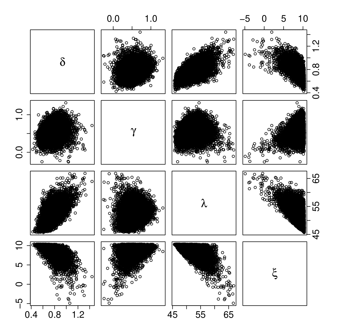
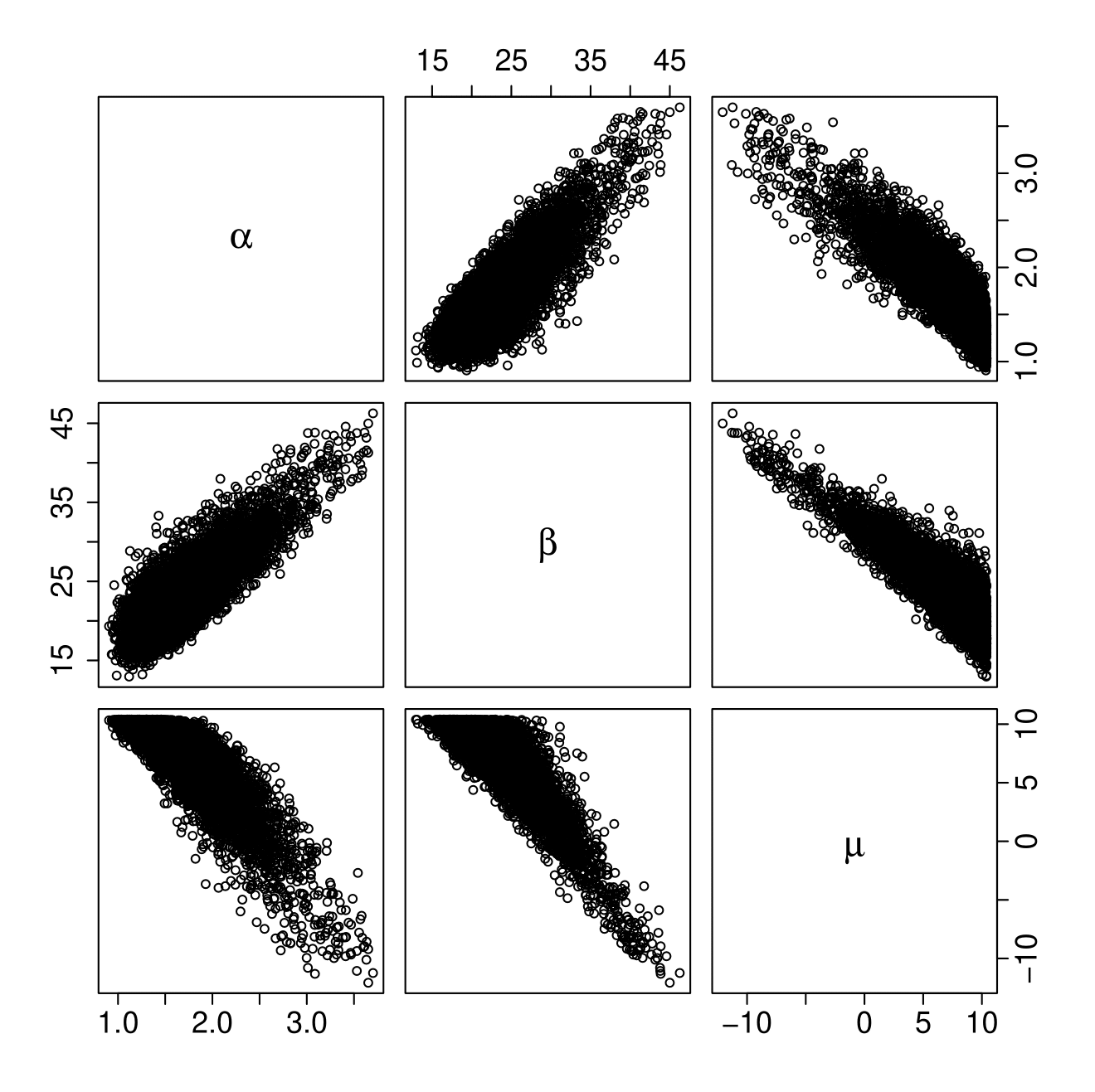
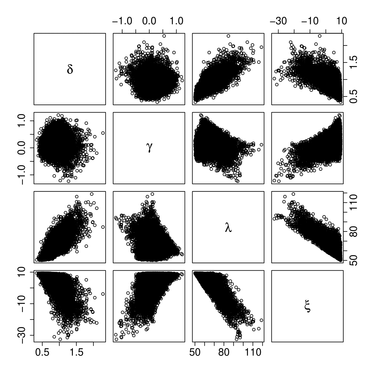
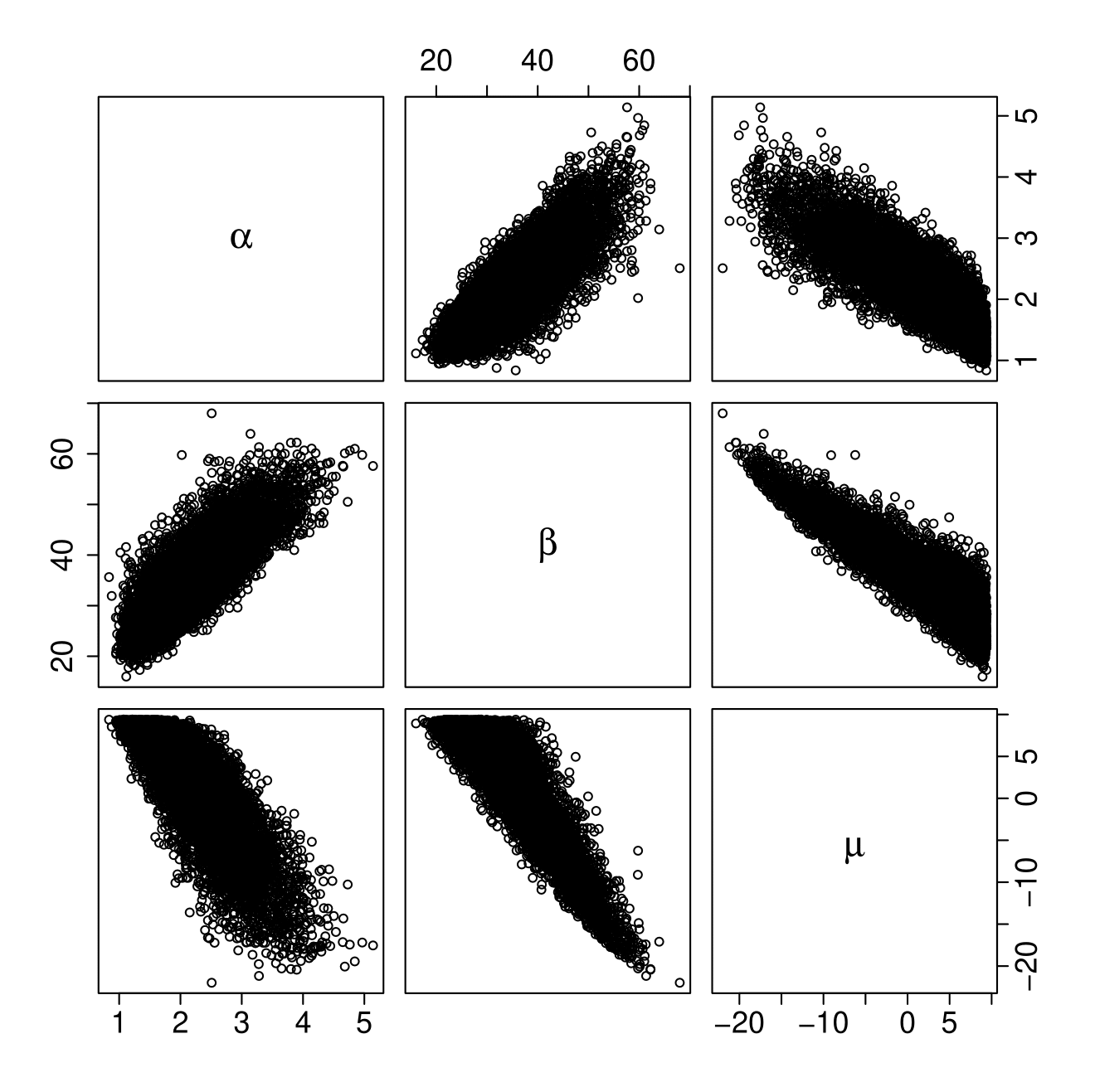
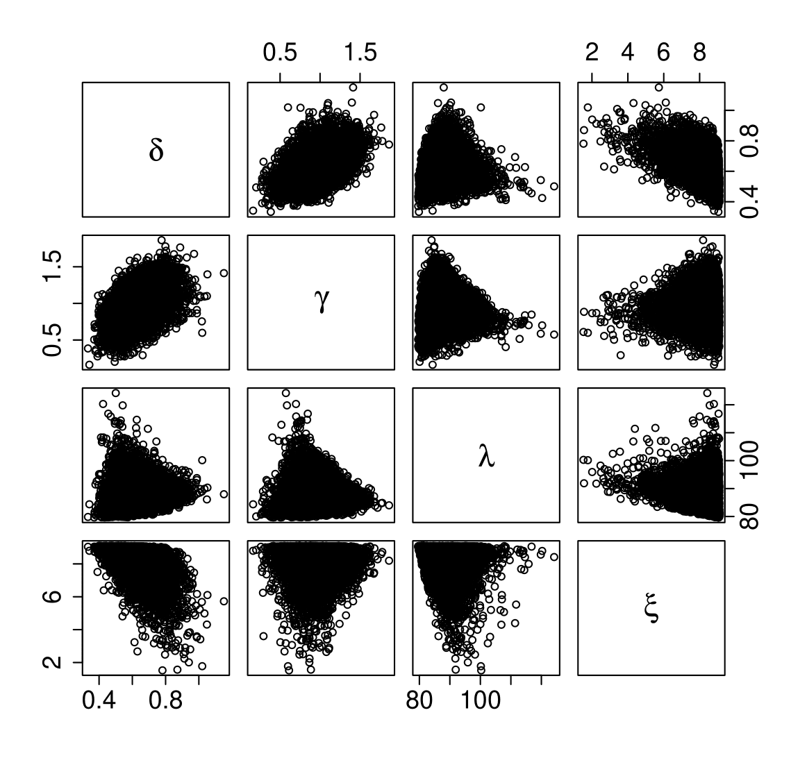
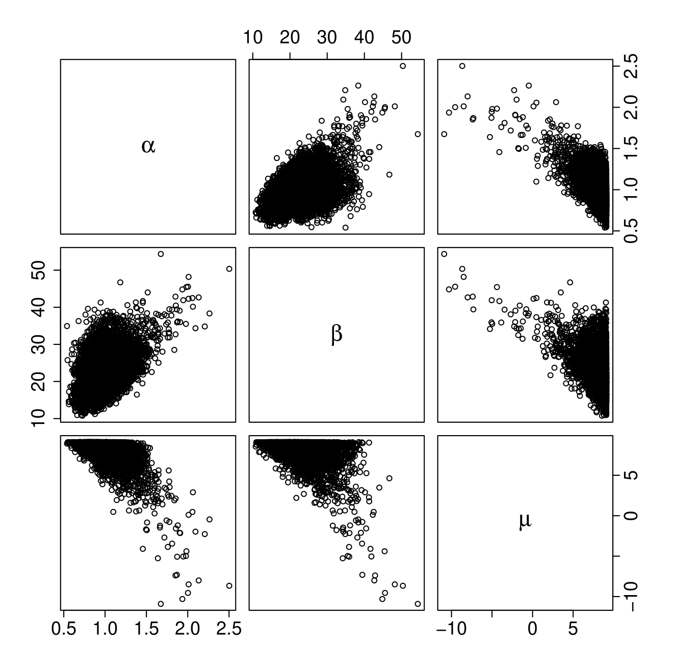
The Bayesian approach were applied to the DBH data addressed in the previous subsection. We compared the performance of the JBS and three-parameter Weibull distributions for modelling DBH data when the parameters of both models were estimated using the Bayesian approach. Figure 1 and Figure 2 display histograms of the samples drawn from the full conditionals and the pairwise scatterplots of the sampler output for the JSB and three-parameter Weibull distributions, respectively, when these distributions fitted to DBH data of the plot 9. Accordingly, Figure 3 and Figure 4 show histograms of the samples drawn from the full conditionals and pairwise scatterplots of the sampler output for the JSB and three-parameter Weibull distributions, respectively, when these distributions fitted to the DBH data in the plot 81. Finally, the graphical visualizations when the JSB and three-parameter Weibull distributions fitted to the DBH data in the plot 73 are shown in Figure 5 and Figure 6, respectively. We assumed that the sampler’s convergence has been attained before 5,000 iterations in all three plots for both the JSB and three-parameter Weibull distributions. Therefore, we removed the first 5000 samples from the sampler output when the sampler were repeated for 10,000 times. Based on the average of the final 5,000 samples, we obtained the Bayesian estimators of the models parameters. The estimated parameters are given in Table 4. The goodness-of-fit statistics including Anderson-Darling (AD), Cramér–von Mises (CM), Kolmogorov-Smirnov (KS), and log-likelihood (LL) statistics were used as criterion for choosing the better model. These criteria are defined as

$$AD =-n-\sum_{i=1}^{n}\frac{2i-1}{n}\biggl[\log G\bigl(x_{(i)}\big|\hat{\Theta}\bigr)+\log\Bigl(1-G\bigl(x_{(n+i-1)}\big|\hat{\Theta}\bigr)\Bigr)\biggr],$$

$$CM =\frac{1}{12n}+\sum_{i=1}^{n}\biggl[G\bigl(x_{(i)}\big|\hat{\Theta}\bigr)-\frac{2i-1}{2n}\biggr]^{2},$$

$$KS =\underset{x_{i}\in{\boldsymbol{x}}}{\operatorname{sup}}\Big|G\bigl(x_{i}\big|\hat{\Theta}\bigr)-G_{n}(x_{i})\Big|,$$

$$LL =\sum_{i=1}^{n}\log g\bigl(x_{i}\big|\hat{\Theta}\bigr),$$

where $G_{n}(.)$ denotes the empirical distribution function, $x_{(i)}$ is th $i$-th order statistic in the random sample of size $n$, and $\hat{\Theta}$ is the estimated vector parameter. The computed goodness-of-fit statistics are given in Table 5. For analyzing the DBH data given in Table 2, we used the R package ForestFit (Teimouri et al. 2020) developed for R (R Core Team 2018) and uploaded to CRAN (Comprehensive R Archive Network) at https://cran.r-project.org/web/packages/Fores
tFit/index.html.

4 Results

The DBH values ranged from 9.1 to 88.6 cm and the mean of DBH ranged between 24.27 and 33.35 cm in DBH (Table 2). The DBH distributions were usually continuous with peaks at the lower, middle, and higher bins (Fig. 7). Mixed forests with ponderosa pine and scattered western junipers are usually a mosaic composed of different forest patches. The analysis of three randomly selected plots represented the following results.

Plot 9 was characterized by DBH distribution that had trees in the size between 10.4 and 55.9 cm in DBH (Fig. 2). The understory cohort was characterized by a distribution with an understory cohort that has one peak around 15 cm in DBH, and truncated at 60 cm in DBH (Figure 7). Overall, the JSB model was the superior model than the Weibull model for DBH distribution (Table 4). The DBH distribution was best captured better by JSB distribution than the Weibull. The JSB was the superior model in the sense of AD, CM, KS, and LL measures (Table 4). The shapes of the fitted distributions to the DBH data of plot 9 were different in the right tail (Fig. 7). In fact, the JSB was characterized the tail of the DBH distribution better than the Weibull distribution.

Plot 44 was characterized by DBH distribution that had trees in the size between 11.9 and 83.8 cm in DBH (Table 2). This plot represented a one-storied forest that was characterized by a DBH distribution with three modes around 15, 35, and 60 cm in DBH. Ignoring these modes, the understory cohort was characterized by a broadly uniform distribution with an understory cohort between 9-60 cm in DBH (Figure 7). Overall, the JSB model was the superior model than the Weibull model for DBH distribution (Table 4). The shape of the fitted densities corresponding to the JSB and Weibull distributions have differences in the middle and the right tail (Figure 7). This is largely because the JSB has two threshold parameters that makes its pdf bounded from the left and right.

Plot 73 was characterized by DBH distribution that had trees in the size between 9.1 and 88.6 cm in DBH (Table 2). This plot was characterized by a generally negative exponential or reverse-J DBH distribution. Overall, this type of DBH distribution occurs in uneven-aged, complex structure, and old-growth forests where the number of trees declines sharply with increasing tree size (Figure 7). There are two peaks around 15 and 35 cm in DBH. In contrast to the plot 9 and 44, the DBH distribution of plot 73 was much wider with a long and skewed to the right tail. The JSB model was characterized the DBH distribution better than the Weibull model (Table 4). Evidently, the JSB was the superior model than the Weibull model for DBH observations at the first peak, between two peaks, and right tail (Figure 7). In all three plots, the JSB outperformed the Weibull model in terms of all AD, CM, KS, and LL measures (Table 4).

5 Discussion

For implementing the Bayesian paradigm, we carried out a study for choosing the initial values. In the case of the JSB distribution, it is known that the first order statistic, i.e., $x_{(1)}$ is a sufficient statistic for $\xi$. So, choosing $\xi^{(0)}=x_{(1)}-1/n$ in which $n$ is the sample size would be quite reasonable as the initial value for $\xi$. In the same fashion as for $\xi$, a good initial value for $\lambda$, since $\xi<x<\xi+\lambda$, is given by $\lambda^{(0)}=x_{(n)}-x_{(1)}+2/n$ in which $x_{(n)}$ is the maximum value of DBH in the sample, i.e., $x_{(n)}$. Here, the constants $1/n$ and $2/n$ for $\xi^{(0)}$ and $\lambda^{(0)}$ has been used to avoid the possible singularity problems. A suitable initial value for $\gamma$ is obtained by considering the relation $\gamma=\delta\log\bigl(1/{\boldsymbol{y}}_{0.5}-1\bigr)$ where ${\boldsymbol{y}}_{0.5}$ is median of the transformation ${\boldsymbol{y}}=({\boldsymbol{x}}-\xi)/\lambda$ with ${\boldsymbol{x}}=\bigl(x_{1},\dots,x_{n}\bigr)^{T}$ (Özçelik et al. 2016). Therefore, $\gamma^{(0)}=\delta^{(0)}\log\bigl(1/{\boldsymbol{y}}_{0.5}-1\bigr)$ where ${\boldsymbol{y}}_{0.5}$ is median of the transformation ${\boldsymbol{y}}=\bigl({\boldsymbol{x}}-\xi^{(0)}\bigr)/\lambda^{(0)}$. It should be noted that we took $\delta^{(0)}=1$ as the initial value for $\delta$.

Additionally, our study revealed that the Bayesian paradigm presented in this work is robust with respect to $\delta^{(0)}$, so that it can be started well away from the true value of $\delta$. In the case of the three-parameter Weibull distribution, similar to the JSB distribution, we used $\xi^{(0)}=x_{(1)}-1/n$ as the initial value for $\mu$. The initial values of the shape and scale parameters obtained by using the method of moments (Norman et al. 1994). We also performed a simulation study to check the robustness of the Bayesian paradigm with respect to the initial values for estimating the parameters of the JSB distribution. For this purpose, we confine ourselves to the case in which we have simulated 300 samples each of size 100 from JSB distribution with parameter vector $\Theta=(2,2,20,0)^{T}$, i.e., $\delta=2$, $\gamma=2$, $\lambda=20$, and $\xi=0$. The results of simulation are given in Table 3. We note that in each of 200 runs, the initial values were not chosen by the method suggested above. Instead, the initial values were generated randomly from uniform distribution. We used this scenario in order to check the robustness of the Gibbs sampler. The initial values for $\delta$, $\gamma$, $\lambda$ ,and $\xi$ were generated from uniform distribution (0.1,15), (-15,15), (20.1,60), and (-10,10), respectively. For example, the general motion of the Gibbs sampler has been shown in Figure 8, when the initial values were chosen as $\delta^{(0)}=15$, $\gamma^{(0)}=-15$, $\lambda^{(0)}=60$, and $\xi^{(0)}=-10$ to show the robustness of the Bayesian paradigm.

6 Conclusion

We have derived the Bayesian estimators for the four-parameter Johnson’s SB (JSB) distribution. The maximum likelihood (ML) approach is the most commonly used method for estimating the model parameters, but it has been shown using simulation study that percentage of failed attempts to reach the convergence through this method is on the average 32%. So, we suggest to use the Bayesian paradigm to estimate the parameters of the JSB distribution. We have shown that the proposed Bayesian approach works efficiently and is robust with respect to the initial values. Furthermore, we have considered the Bayesian estimators for parameters of the three-parameter Weibull distribution that proposed by Green et al. (1994). Our algorithm for sampling from full conditional of the location parameter is faster to that of Green et al. (1994). The We have fitted both of the JSB and three-parameter Weibull distributions to the diameters at breast height (DBH) obtained from 3 plots out of 107 plots of size 0.08 ha established in mixed-age ponderosa pine (Pinus ponderosa Dougl. ex Laws.) forests with scattered western junipers located in the Malheur National Forest on the south end of the Blue Mountains near Burns, Oregon, USA. The estimation results indicated that the JBS model outperformed the three-parameter Weibull distribution and so characterized more accurately the DBH distribution. As a possible future work, we are interested in estimating the parameters of the bivariate JSB distribution using the Bayesian method. The users can access the R package ForestFit that is available at address https://cran.r-project.org/web/packages/ForestFit/index.html.

Appendix A

We have

$$\pi(\delta|\gamma,\lambda,\xi,\boldsymbol{x}) \propto\frac{\delta^{n}\lambda^{n}}{(2\pi)^{\frac{n}{2}}\Pi_{i=1}^{n}(x_{i}-\xi)(\lambda+\xi-x_{i})}\exp\left\{-\frac{1}{2}\sum_{i=1}^{n}\Bigg[\gamma+\delta\log\biggl(\frac{x_{i}-\xi}{\lambda+\xi-x_{i}}\biggr)\Bigg]^{2}\right\}$$

$$\propto\delta^{n}\exp\left\{-\frac{k_{2}}{2}\biggl[\delta+\frac{\gamma k_{1}}{k_{2}}\biggr]^{2}\right\},$$

where

$$k_{1}=\sum_{i=1}^{n}\log\Bigl(\frac{x_{i}-\xi}{\lambda+\xi-x_{i}}\Bigr),$$ (11)

and

$$k_{2}=\sum_{i=1}^{n}\bigg[\log\Bigl(\frac{x_{i}-\xi}{\lambda+\xi-x_{i}}\Bigr)\biggr]^{2}.$$ (12)

The full conditional pdf of $\delta$ is given by

$$\pi(\delta|\gamma,\lambda,\xi,\boldsymbol{x})=\text{C}\delta^{n}\exp\left\{-\frac{k_{2}}{2}\biggl[\delta+\frac{\gamma k_{1}}{k_{2}}\biggr]^{2}\right\},$$

where C is a normalizing constant independent of $\delta$. The First and second derivatives of $\log\pi(\delta|\gamma,\lambda,\xi,\boldsymbol{x})$ with respect to $\delta$ are

$$\frac{\partial\pi(\delta|\gamma,\lambda,\xi,\boldsymbol{x})}{\partial\delta}=\frac{n}{\delta}-k_{2}\biggl[\delta+\frac{\gamma k_{1}}{k_{2}}\biggr],$$

and

$$\frac{\partial^{2}\pi(\delta|\gamma,\lambda,\xi,\boldsymbol{x})}{\partial\delta^{2}}=-\frac{n}{\delta^{2}}-k_{2}.$$ (13)

Since $k_{2}>0$, the right-hand side of (13) is always negative and so $\pi(\delta|\gamma,\lambda,\xi,\boldsymbol{x})$ is log-concave. Assume that we are currently at $t$-th iteration of the sampler, sampling from $\pi\bigl(\delta\big|\gamma^{(t)},\lambda^{(t)},\xi^{(t)},\boldsymbol{x}\bigr)$ is carried out through the ARS algorithm. Here, $\gamma^{(t)}$, $\lambda^{(t)}$, and $\xi^{(t)}$ denote the generated values, respectively, from $\gamma$, $\lambda$, and $\xi$, at $t$-th iteration.

Appendix B

We have

$$\pi(\gamma|\delta,\lambda,\xi,\boldsymbol{x})\propto\exp\left\{-\frac{1}{2}\sum_{i=1}^{n}\Bigg[\gamma+\delta\log\biggl(\frac{x_{i}-\xi}{\lambda+\xi-x_{i}}\biggr)\Bigg]^{2}\right\}\propto\exp\left\{-\frac{n}{2}\biggl[\gamma+\frac{\delta k_{1}}{n}\biggr]^{2}\right\},$$

where $k_{1}$ is defined in (11). Assume that we are currently at $t$-th iteration of the sampler, for sampling from full conditional pdf of $\gamma$, it is enough to sample from Gaussian distribution with mean

$$-\frac{\delta^{(t+1)}}{n}\sum_{i=1}^{n}\log\biggl(\frac{x_{i}-\xi^{(t)}}{\lambda^{(t)}+\xi^{(t)}-x_{i}}\biggr),$$

and variance $1/n$.

Appendix C

It is easy to see that the full conditional of $\lambda$ is (up to proportionality)

$$\pi(\lambda|\delta,\gamma,\xi,\boldsymbol{x}) \propto\Pi_{i=1}^{n}\biggl(\frac{\lambda}{\lambda+\xi-x_{i}}\biggr)\exp\left\{-\frac{1}{2}\sum_{i=1}^{n}\Bigg[\gamma+\delta\log\biggl(\frac{x_{i}-\xi}{\lambda+\xi-x_{i}}\biggr)\Bigg]^{2}\right\}$$

$$=\lambda^{n}\Pi_{i=1}^{n}\Bigl(\lambda+\xi-x_{i}\Bigr)^{\delta\gamma-1}\exp\left\{-\frac{\delta^{2}}{2}\sum_{i=1}^{n}\Bigg[\log\biggl(\frac{x_{i}-\xi}{\lambda+\xi-x_{i}}\biggr)\Bigg]^{2}\right\},$$

As it is seen, the structure of the full conditional pdf of $\lambda$ is complicated. Additionally, $\pi(\lambda|\delta,\gamma,\xi,\boldsymbol{x})$ is not always log-concave. So, we use the MH algorithm for sampling from $\pi(\lambda|\delta,\gamma,\xi,\boldsymbol{x})$ by choosing $\exp\Bigl\{-\bigl(\lambda-x_{(n)}+\xi\bigr)\Bigr\}$ as the proposal pdf for $\lambda>x_{(n)}-\xi$ wherein $x_{(n)}=\max\{x_{1},\dots,x_{n}\}$. The six-step MH algorithm is given a follows.

1. Suppose we are currently at $t$-th iteration of the sampler. Choose the initial value as $\lambda_{(0)}=x_{(n)}-\xi^{(t)}+1/n$ and set i=1;

2. Sample $\lambda^{*}$ from proposal distribution $q\bigl(\lambda)$ with pdf $\exp\Bigl\{-\bigl(\lambda-x_{(n)}+\xi^{(t)}\bigr)\Bigr\}$, for $\lambda>x_{(n)}-\xi^{(t)}$;

3. Compute $\eta$ as

   $$\eta=\min\left\{1,\frac{\pi\bigl(\lambda_{*}\big|\delta^{(t+1)},\gamma^{(t+1)},\xi^{(t)},\boldsymbol{x}\bigr)\exp\bigl\{-\lambda_{(i-1)}\bigr\}}{\pi\bigl(\lambda_{(i-1)}\big|\delta^{(t+1)},\gamma^{(t+1)},\xi^{(t)},\boldsymbol{x}\bigr)\exp\bigl\{-\lambda_{*}\bigr\}}\right\}.$$

4. Generate an uniform random variable on $(0,1)$, say $u$. If $u<\eta$, then $\lambda_{(i)}=\lambda_{*}$, otherwise $\lambda_{(i)}=\lambda_{(i-1)}$;

5. If $i=N$, then go to the next step. Otherwise set $i=i+1$ and go to step 2;

6. Accept $\lambda_{(N)}$ as a generation form $\pi\bigl(\lambda\big|\delta^{(t)},\gamma^{(t)},\xi^{(t)},\boldsymbol{x}\bigr)$, i.e., $\lambda^{(t+1)}=\lambda_{(N)}$ and stop the MH algorithm.

Appendix D

Similar to the $\lambda$, the full conditional pdf of $\xi$ has complicated structure. We have

$$\pi(\xi|\delta,\gamma,\lambda,\boldsymbol{x}) \propto\Pi_{i=1}^{n}\Biggl(\frac{(\lambda+\xi-x_{i})^{\delta\gamma-1}}{(x_{i}-\xi)^{\delta\gamma+1}}\Biggr)\exp\left\{-\frac{\delta^{2}}{2}\sum_{i=1}^{n}\Bigg[\log\biggl(\frac{x_{i}-\xi}{\lambda+\xi-x_{i}}\biggr)\Bigg]^{2}\right\},$$

where $x_{(n)}-\lambda<\xi<x_{(1)}$ in which $x_{(1)}=\min\{x_{1},\dots,x_{n}\}$. Since the full conditional pdf of $\xi$ is not always log-concave, so we use the MH algorithm to sample from it. For this aim, we choose the uniform distribution on $\bigl(x_{(n)}-\lambda,x_{(1)}\bigr)$ as the proposal. The six-step MH algorithm is given by the following.

1. Suppose we are currently at $t$-th iteration of the sampler. Set $i=1$ and generate a random variable from uniform distribution on $\bigl(x_{(n)}-\lambda^{(t+1)},x_{(1)}\bigr)$, say $u$. Set $u=\xi^{(0)}$;

2. Sample $\xi^{*}$ from proposal distribution with pdf $q\bigl(\xi)=1/\bigl(x_{(1)}-x_{(n)}+\lambda^{(t+1)}\bigr)$;

3. Compute $\eta$ as

   $$\eta=\min\left\{1,\frac{\pi\bigl(\xi^{*}\big|\delta^{(t+1)},\gamma^{(t+1)},\lambda^{(t+1)},\boldsymbol{x}\bigr)}{\pi\bigl(\xi^{(i-1)}\big|\delta^{(t+1)},\gamma^{(t+1)},\lambda^{(t+1)},\boldsymbol{x}\bigr)}\right\}.$$

4. Generate an uniform random variable, say $u$, on $(0,1)$. If $u<\eta$, then $\xi^{(i)}=\xi^{*}$, otherwise $\xi^{(i)}=\xi^{(i-1)}$;

5. If $i=N$, then go to the next step. Otherwise set $i=i+1$ and go to step 2;

6. Accept $\xi_{(N)}$ as a generation form pdf $\pi\Bigl(\xi\big|\delta^{(t+1)},\gamma^{(t+1)},\lambda^{(t+1)},\boldsymbol{x}\Bigr)$, i.e., $\xi^{(t+1)}=\xi_{(N)}$ and stop the MH algorithm.

Table 1: Percentage of runs that NR method truly converged for the JSB distribution.

Sample size	20	50	100	250	500	1000	5000
Percentage	68.5%	68.7%	68.3%	68.3%	68.1%	68.4%	67.9%

Table 2: Summary statistics for DBH data.

Plot	Plot size	Min	1st Quar.	Median	Mean	3rd Quar.	Max.	St.Dev.	Skewness
9	52	10.4	17.32	27.55	28.01	36.42	55.9	12.37	0.48
44	42	11.9	14.78	17.40	24.27	26.50	83.8	15.06	2.13
73	35	9.1	13.85	21.10	30.35	39.75	88.6	20.94	1.15

Table 3: Descriptive statistics for the sampler output.

Parameter	Min	1st Quar.	Median	Mean	3rd Quar.	Max.	St.Dev.	Skewness
$\delta$	1.242	1.724	1.850	1.874	1.996	15.000	0.3406	20.123
$\gamma$	-15.000	1.407	1.615	1.609	1.804	15.982	0.450	7.225
$\lambda$	12.399	15.941	17.215	17.155	18.410	60.000	1.719	1.469
$\xi$	-10.000	-0.1270	0.245	0.160	0.549	1.399	0.542	-1.460

Table 4: Bayesian estimators for the parameters of the JBS and three-parameter Weibull distributions.

	JSB distribution					Weibull distribution
Plot	${\delta}$	${\gamma}$	${\lambda}$	$\xi$		$\alpha$	$\beta$	$\mu$
9	0.772	0.545	52.311	8.719		1.682	23.120	7.436
44	0.875	0.203	64.162	3.642		2.145	34.496	2.171
73	0.641	0.978	88.592	8.182		1.005	22.746	8.278

Table 5: Computed goodness-of-fit statistics for modelling DBH data using JBS and three-parameter Weibull distributions.

	JSB distribution					Weibull distribution
Plot	AD	CM	KS	LL		AD	CM	KS	LL
9	0.167	0.023	0.059	-196.808		0.310	0.048	0.082	-199.579
44	0.216	0.028	0.100	-120.072		0.302	0.040	0.115	-121.846
73	0.105	0.031	0.075	-141.751		0.257	0.045	0.084	-143.299

Figure 1: Left-hand side: pairwise scatterplots of trimmed output of the Gibbs sampler for estimation parameters of the JSB distribution fitted to the DBH observations in plot 9. These outputs suggest that there is little dependence between $\delta$ and $\lambda$. Right-hand side: histograms of the full conditionals (a) $\pi(\delta|\gamma,\lambda,\xi,\boldsymbol{x})$, (b) $\pi(\gamma|\delta,\lambda,\xi,\boldsymbol{x})$, (c) $\pi(\lambda|\delta,\gamma,\xi,\boldsymbol{x})$, and (d) $\pi(\xi|\delta,\gamma,\lambda,\boldsymbol{x})$ produced by the Gibbs sampler for 10,000 runs.

Figure 2: Left-hand side: pairwise scatterplots of trimmed output of the Gibbs sampler for estimation parameters of the three-parameter Weibull distribution fitted to the DBH observations in plot 9. These outputs suggest that there is considerable dependence between all pairs. Right-hand side: histograms of the full conditionals (a) $\pi(\alpha|\beta,\mu,\boldsymbol{x})$, (b) $\pi(\beta|\alpha,\mu,\boldsymbol{x})$, and (c) $\pi(\mu|\alpha,\beta,\boldsymbol{x})$ produced by the Gibbs sampler for 10,000 runs.

Figure 3: Left-hand side: pairwise scatterplots of trimmed output of the Gibbs sampler for estimation parameters of the JSB distribution fitted to the DBH observations in plot 44. These outputs suggest that there is little dependence between between pairs $(\delta,\lambda)$ and $(\lambda,\xi)$. Right-hand side: histograms of the full conditionals (a) $\pi(\delta|\gamma,\lambda,\xi,\boldsymbol{x})$, (b) $\pi(\gamma|\delta,\lambda,\xi,\boldsymbol{x})$, (c) $\pi(\lambda|\delta,\gamma,\xi,\boldsymbol{x})$, and (d) $\pi(\xi|\delta,\gamma,\lambda,\boldsymbol{x})$ produced by the Gibbs sampler for 10,000 runs.

Figure 4: Left-hand side: pairwise scatterplots of trimmed output of the Gibbs sampler for estimation parameters of the three-parameter Weibull distribution fitted to the DBH observations in plot 44. These outputs suggest that there is considerable dependence between all pairs. Right-hand side: histograms of the full conditionals (a) $\pi(\alpha|\beta,\mu,\boldsymbol{x})$, (b) $\pi(\beta|\alpha,\mu,\boldsymbol{x})$, and (c) $\pi(\mu|\alpha,\beta,\boldsymbol{x})$ produced by the Gibbs sampler for 10,000 runs.

Figure 5: Left-hand side: pairwise scatterplots of trimmed output of the Gibbs sampler for estimation parameters of the JSB distribution fitted to the DBH observations in plot 73. These outputs suggest that there is little dependence between $\delta$ and $\gamma$. Right-hand side: histograms of the full conditionals (a) $\pi(\delta|\gamma,\lambda,\xi,\boldsymbol{x})$, (b) $\pi(\gamma|\delta,\lambda,\xi,\boldsymbol{x})$, (c) $\pi(\lambda|\delta,\gamma,\xi,\boldsymbol{x})$, and (d) $\pi(\xi|\delta,\gamma,\lambda,\boldsymbol{x})$ produced by the Gibbs sampler for 10,000 runs.

Figure 6: Left-hand side: pairwise scatterplots of trimmed output of the Gibbs sampler for estimation parameters of the three-parameter Weibull distribution fitted to the DBH observations in plot 73. These outputs suggest that there is little dependence between $\alpha$ and $\mu$. Right-hand side: histograms of the full conditionals (a) $\pi(\alpha|\beta,\mu,\boldsymbol{x})$, (b) $\pi(\beta|\alpha,\mu,\boldsymbol{x})$, and (c) $\pi(\mu|\alpha,\beta,\boldsymbol{x})$ produced by the Gibbs sampler for 10,000 runs.

Figure 7: Histograms of DBH data in plots 9, 44, and 73. Superimposed in each subfigure are estimated probability density functions of the JSB (blue solid line) and Weibull (red dashed line) distributions.

Figure 8: Output of (a) $\delta$, (b) $\gamma$, (c) $\lambda$, and (d) $\xi$ from Gibbs sampler for the robust analysis. Each subfigure shows the motion of the Gibbs sampler across 10,000 iterations.

References

- Bailey and Dell (1973) Bailey, R.L., Dell, T., 1973. Quantifying diameter distributions with the Weibull function. Forest Science 19, 97–104.
- Fonseca et al. (2009) Fonseca, T.F., Marques, C.P., Parresol, B.R., 2009. Describing maritime pine diameter distributions with Johnson’s SB distribution using a new all-parameter recovery approach. Forest Science 55, 367–373.
- Gilks and Wild (1992) Gilks, W.R., Wild, P., 1992. Adaptive rejection sampling for Gibbs sampling. Journal of the Royal Statistical Society: Series C (Applied Statistics) 41, 337–348.
- Gorgoso et al. (2007) Gorgoso, J., González, J.Á., Rojo, A., Grandas-Arias, J., 2007. Modelling diameter distributions of betula alba l. stands in northwest Spain with the two-parameter Weibull function. Forest Systems 16, 113–123.
- Gorgoso et al. (2012) Gorgoso, J., Rojo, A., Cámara-Obregón, A., Diéguez-Aranda, U., 2012. A comparison of estimation methods for fitting Weibull, Johnson’s SB and beta functions to Pinus pinaster, Pinus radiate and Pinus sylvestris stands in northwest Spain. Forest Systems 21, 446–459.
- Gove et al. (2008) Gove, J.H., Ducey, M.J., Leak, W.B., Zhang, L., 2008. Rotated sigmoid structures in managed uneven-aged northern hardwood stands: a look at the Burr type III distribution. Forestry 81, 161–176.
- Green et al. (1994) Green, E.J., Roesch Jr, F.A., Smith, A.F., Strawderman, W.E., 1994. Bayesian estimation for the three-parameter Weibull distribution with tree diameter data. Biometrics , 254–269.
- Hafley and Buford (1985) Hafley, W., Buford, M., 1985. A bivariate model for growth and yield prediction. Forest Science 31, 237–247.
- Hafley and Schreuder (1977) Hafley, W., Schreuder, H., 1977. Statistical distributions for fitting diameter and height data in even-aged stands. Canadian Journal of Forest Research 7, 481–487.
- Jeffreys (1961) Jeffreys, H., 1961. Theory of Probability. Oxford University Press London.
- Johnson (1949) Johnson, N.L., 1949. Systems of frequency curves generated by methods of translation. Biometrika 36, 149–176.
- Kerns et al. (2017) Kerns, B.K., Westlind, D.J., Day, M.A., 2017. Season and interval of burning and cattle exclusion in the southern Blue Mountains, Oregon: Overstory tree height, diameter and growth. USDA Forest Service Research Data Archive, https://doi.org/10.2737/RDS-2017-0041 .
- Kiviste et al. (2003) Kiviste, A., Nilson, A., Hordo, M., Merenäkk, M., 2003. Diameter distribution models and height-diameter equations for Estonian forests. Modelling Forest Systems , 169–179.
- Kudus et al. (1999) Kudus, K.A., Ahmad, M., Lapongan, J., 1999. Nonlinear regression approach to estimating Johnson SB parameters for diameter data. Canadian Journal of Forest Research 29, 310–314.
- Maltamo et al. (2000) Maltamo, M., Kangas, A., Uuttera, J., Torniainen, T., Saramäki, J., 2000. Comparison of percentile based prediction methods and the Weibull distribution in describing the diameter distribution of heterogeneous Scots pine stands. Forest Ecology and Management 133, 263–274.
- Maltamo et al. (1995) Maltamo, M., Puumalainen, J., Päivinen, R., 1995. Comparison of beta and Weibull functions for modelling basal area diameter distribution in stands of pinus sylvestris and picea abies. Scandinavian Journal of Forest Research 10, 284–295.
- Marto et al. (2009) Marto, M., Palma, J., Mateus, A., Tomé, M., 2009. Computer program for estimation of Johnson’s SB parameters using a parameter recovery method. Publicações Científicas Forchange PC-X/2009. Centro de Estudos Florestais, Instituto Superior de Agronomia, Universidade Técnica de Lisboa, Lisboa .
- Mateus and Tomé (2011) Mateus, A., Tomé, M., 2011. Modelling the diameter distribution of eucalyptus plantations with Johnson’s SB probability density function: parameters recovery from a compatible system of equations to predict stand variables. Annals of Forest Science 68, 325–335.
- Nagatsuka et al. (2013) Nagatsuka, H., Kamakura, T., Balakrishnan, N., 2013. A consistent method of estimation for the three-parameter Weibull distribution. Computational Statistics & Data Analysis 58, 210–226.
- Norman et al. (1994) Norman, L.J., Kotz, S., Balakrishnan, N., 1994. Continuous Univariate Distributions. volume I. John Wiley & Sons.
- Özçelik et al. (2016) Özçelik, R., Fidalgo Fonseca, T.J., Parresol, B.R., Eler, Ü., 2016. Modeling the diameter distributions of Brutian Pine stands using Johnson’s SB distribution. Forest Science 62, 587–593.
- Palahí et al. (2007) Palahí, M., Pukkala, T., Blasco, E., Trasobares, A., 2007. Comparison of beta, Johnson’s SB, Weibull and truncated Weibull functions for modeling the diameter distribution of forest stands in Catalonia (north-east of Spain). European Journal of Forest Research 126, 563–571.
- Parresol (2003) Parresol, B.R., 2003. Recovering parameters of Johnson’s SB distribution. Res. Pap. SRS-31. Asheville, NC: US Department of Agriculture, Forest Service, Southern Research Station. 9 p. 31.
- Pretzsch (2009) Pretzsch, H., 2009. Forest dynamics, growth, and yield, in: Forest dynamics, growth and yield. Springer, pp. 1–39.
- R Core Team (2018) R Core Team, 2018. R: A Language and Environment for Statistical Computing. R Foundation for Statistical Computing. Vienna, Austria. URL: https://www.R-project.org/.
- Rennolls and Wang (2005) Rennolls, K., Wang, M., 2005. A new parameterization of Johnson’s SB distribution with application to fitting forest tree diameter data. Canadian Journal of Forest Research 35, 575–579.
- Robert et al. (2010) Robert, C.P., Casella, G., Casella, G., 2010. Introducing Monte Carlo methods with R. volume 18. Springer.
- Roberts and Smith (1994) Roberts, G.O., Smith, A.F., 1994. Simple conditions for the convergence of the Gibbs sampler and Metropolis-Hastings algorithms. Stochastic Processes and Their Applications 49, 207–216.
- Scolforo et al. (2003) Scolforo, J.R.S., Tabai, F.C.V., de Macedo, R.L.G., Acerbi Jr, F.W., de Assis, A.L., 2003. SB distribution’s accuracy to represent the diameter distribution of Pinus taeda, through five fitting methods. Forest Ecology and Management 175, 489–496.
- Smith and Naylor (1987) Smith, R.L., Naylor, J., 1987. A comparison of maximum likelihood and Bayesian estimators for the three-parameter weibull distribution. Journal of the Royal Statistical Society: Series C (Applied Statistics) 36, 358–369.
- Teimouri et al. (2020) Teimouri, M., Doser, J.W., Finley, A.O., 2020. Forestfit: An R package for modeling plant size distributions. Environmental Modelling & Software , 104668.
- Zhang et al. (2003) Zhang, L., Packard, K.C., Liu, C., 2003. A comparison of estimation methods for fitting Weibull and Johnson’s SB distributions to mixed spruce fir stands in northeastern North America. Canadian Journal of Forest Research 33, 1340–1347.
- Zhang et al. (2010) Zhang, X., Lei, Y., Cao, Q.V., 2010. Compatibility of stand basal area predictions based on forecast combination. Forest Science 56, 552–557.
- Zhou and McTague (1996) Zhou, B., McTague, J.P., 1996. Comparison and evaluation of five methods of estimation of the Johnson system parameters. Canadian Journal of Forest Research 26, 928–935.