Virus Dynamics with Behavioral Responses

Abstract

Motivated by epidemics such as COVID-19, we study the spread of a contagious disease when people change their behavior to respond to the disease prevalence. We extend the SIR epidemiological model to include endogenous meeting rates. Individuals benefit from economic activity, but higher activity also leads to more interactions with potentially infected individuals. The main focus is a theoretical analysis of the contagion dynamics. In the leading case, the infection prevalence is single-peaked. We obtain a simple condition for when several types of public-health interventions or changes in disease prevalence will paradoxically increase infection rates due to risk compensation. This condition implies that public-health interventions are most likely to be undermined by increased economic activity near the peak of severe diseases.

1 Introduction

In severe epidemics such as COVID-19, the spread of contagious diseases depends substantially on behavioral and policy responses. Standard epidemiological models predict diseases paths under several assumptions on social distancing, and outcomes usually differ dramatically across these scenarios. Given the very large impact of mitigation measures such as social distancing on infection dynamics, understanding how much people will interact is an important open question (Funk et al., 2015).

This paper studies the spread of a disease and the resulting behavioral responses analytically. To analyze the spread of a diseases and the accompanying behavioral responses, we adapt the widely-used SIR epidemiological model to allow individuals to choose activity levels at each point in time. Higher activity levels correspond to actions such as going to work or school which provide economic and social benefits. On the other hand, higher activity also leads to more interactions with potentially infected individuals, especially when the disease prevalence is high and whether others are more active (e.g., public spaces are crowded). Given the shares of the population that are susceptible and infected at a given time, individuals’ choices are determined by a simple game-theoretic framework.

We study the dynamics of the infection and the corresponding behavioral responses. The baseline model considers rational behavior in the absence of policy interventions. In the leading case, disease prevalence is single-peaked: the prevalence initially increases, but then peaks and falls toward zero as behavioral responses and herd immunity slow the spread. Part of the population will eventually be immune while others will never be infected, and the relative sizes of these two groups depend on model parameters and potential policy interventions. In particular, interventions to ‘flatten the curve’ can also affect the share of the population that must be infected before herd immunity reduces a diseases’ spread to very low levels.

With endogenous behavior, policy changes that decrease the transmission rate or the cost of the disease can be offset by decreased social distancing. Indeed, previous models (beginning with Kremer, 1996) have suggested public-health interventions to decrease transmissivity could actually increase infection rates. The logic is that individuals respond to a decrease in risk by increasing activities levels, and this can increase the infection rate under equilibrium behavior. A dynamic model lets us determine whether and when in the course of a disease this may be the case. We identify a region, which has a simple characterization in terms of model parameters, in which behavioral responses to various changes in policies or disease levels are sufficiently strong to produce such paradoxical effects. This region requires a severe disease and a high prevalence. So near the peak of a severe outbreak, public-health interventions can be less effective or even counterproductive unless paired with attempts to maintain social distancing. When prevalence is lower, changes such as requiring masks are quite effective.

1.1 Related Literature

Much of behavioral epidemiology focuses on individuals’ binary choices, such as vaccination, rather than more continuous choices of how much to interact with others (see Manfredi and D’Onofrio, 2013 for several examples of models). This is especially relevant for less severe or less contagious diseases. For example, for influenza in ordinary years, vaccination choices are likely the most relevant behavioral margin for most individuals. But when individuals are engaged in substantial social distancing, choice sets are much richer.

Several models of HIV/AIDS epidemics allow individuals to choose numbers of sexual partners (see Kremer, 1996, Auld, 2003, Greenwood, Kircher, Santos, and Tertilt, 2019, and others). We note three key differences from our model. First, this literature treats HIV/AIDS is treated as an endemic disease at steady state. By contrast, we argue that infection dynamics are important for outbreaks such as COVID-19, which led to dramatic shifts in behavior. Second, HIV/AIDS modeling uses SI rather than SIR model, as infection is an absorbing state and there is no recovery. Third, individuals directly choose a number of partners, i.e., the matching technology is linear rather than quadratic.

Most recently, a number of economists have incorporated endogenous behavior into numerical analyses of SIR models of COVID-19. These models, such as Farboodi, Jarosch, and Shimer (2020), Eichenbaum, Rebelo, and Trabandt (2020), Kruger, Uhlig, and Xie (2020), and Korinek and Bethune (2020), focus largely on macroeconomic consequences of epidemics, and therefore include additional features such as forward-looking agents and production sectors. While we also conduct numerical analysis, our focus is on the theoretical properties of a related model. A major takeaway from our analysis is that basic qualitative properties of disease dynamics and impulse responses can be reversed by changes in model parameters. So careful calibration and/or robustness checks are important in related numerical exercises.

2 Model

2.1 Setup

We consider a model in continuous time, indexed by $t\in[0,\infty)$, with a unit mass of individuals. Individuals can be susceptible, infected, or recovered. We denote the shares of susceptible, infected, and recovered individuals at time $t$ by $S(t),I(t)$, and $R(t)$, respectively.

Each individual chooses a level of activity $q(t)$ to maximize her expected flow payoffs at time $t$. The flow payoffs from activity are

$$q(t)-aq(t)^{2},$$

where $a>0$. This captures economic and social value from actions that can involve meeting other people, such as going to work or school. The marginal value of these actions is decreasing, and absent infection individuals will choose the finite level of activity $\overline{q}=\frac{1}{2a}$. A susceptible individual pays instantaneous cost $C\geq 0$ if infected.

We now describe the infection process. When levels of activity are $(q_{S}(t),q_{I}(t),q_{R}(t))$, an individual choosing level of activity rate $q_{i}(t)$ meets susceptible individuals at Poisson rate $q_{i}(t)q_{S}(t)S(t)$, infected individuals at rate $q_{i}(t)q_{I}(t)I(t)$, and recovered individuals at rate $q_{i}(t)q_{R}(t)R(t)$. All meetings are independent.

When a susceptible individual meets an infected individual, she becomes infected with transmission probability $\beta>0$. Infected individuals recover at Poisson rate $\kappa$, and then are immune in all future periods.

When $C=0$, all individuals choose $q(t)=\overline{q}$ and the model reduces to the standard SIR model. For $C>0$, the meeting rates between individuals will depend on choices of $q(t).$

2.2 Equilibrium

A sequence of (symmetric) actions is given by $(q_{S}(t),q_{I}(t),q_{R}(t))_{t=0}^{\infty}$.

Recovered individuals know that they are recovered. Susceptible and infected individuals know that they have not recovered but not whether they are infected, and therefore believe they are susceptible with probability $\frac{S(t)}{S(t)+I(t)}$ and infected with probability $\frac{I(t)}{S(t)+I(t)}$ at time $t$. Our interpretation is that infected individuals are pre-symptomatic but can spread the disease. We will discuss a model with equivalent dynamics which also includes symptomatic individuals in Remark 1.

Susceptible and infected individuals therefore face the same decision problems. So it will be without loss of generality to consider sequences of actions such that $q_{S}(t)=q_{I}(t)$ for all $t$, and any such sequence is characterized by $(q_{S}(t),q_{R}(t))_{t=0}^{\infty}$.

A sequence of actions is an equilibrium if all individuals choose levels of activity to maximize flow payoffs at all times, given the population distribution and others actions:

Definition 1.

An equilibrium given initial conditions $(S(0),I(0),R(0))$ is a sequence of actions $(q_{S}(t),q_{R}(t))_{t=0}^{\infty}$ such that for all $t$

$$q_{S}(t)=\text{argmax}_{q}q-aq^{2}-Cqq_{S}(t)\beta\cdot\frac{I(t)S(t)}{S(t)+I(t)}\text{ and }q_{R}(t)=\text{argmax}_{q}q(t)-aq(t)^{2}.$$

We now explain the infection costs in the definition. An individual $i$ choosing level of activity $q_{i}(t)$ at time $t$ meets infected individuals at rate $q_{i}(t)q_{S}(t)I(t)$, and meetings with susceptible and recovered individuals are not relevant for $i$’s payoffs. If individual $i$ is not yet recovered, then she believes she is susceptible with probability $\frac{S(t)}{S(t)+I(t)}$ and already infected otherwise. Since the transmission rate is $\beta$, she would be infected by a meeting with an infected individual at time $t$ with probability $\beta\cdot\frac{S(t)}{S(t)+I(t)}$. The expected rate of infection is therefore $q_{i}(t)q_{S}(t)\beta\cdot\frac{I(t)S(t)}{S(t)+I(t)}$, as in the definition above. If the individual is recovered, there are no infection costs.

Remark 1.

Under the quadratic matching assumption, the behavior of recovered individuals does not effect equilibrium behavior by susceptible individuals or the infection rate. Thus, our model is equivalent to a number of extensions with additional heterogeneity.

As one example, infected individuals could be replaced by asymptomatic and symptomatic individuals, where symptomatic individuals choose $q(t)=0$ to avoid spreading the disease. In this case, asymptomatic individuals would be come symptomatic at a Poisson rate. A second example is including a death rate for infected individuals, so that there are two absorbing states.

3 Dynamics

Recovered individuals choose $q_{R}(t)=\overline{q}$ for all $t$, where $\overline{q}=\frac{1}{2a}$. Therefore, an equilibrium is characterized by the level of activity $q_{S}(t)\leq\overline{q}$ for susceptible and infected individuals, which we will refer to as $q(t)$ from now on.

An individual who is susceptible or infected chooses $q_{i}(t)$ to maximize

$$q_{i}(t)-aq_{i}(t)^{2}-C\beta q_{i}(t)q(t)\cdot\frac{I(t)S(t)}{S(t)+I(t)}.$$

Taking the first-order condition for $q_{i}(t)$ and substituting $q_{i}(t)=q(t)$, we obtain

$$q(t)=\frac{1}{2a+C\beta\cdot\frac{I(t)S(t)}{S(t)+I(t)}}$$ (1)

This expression implies that the lexvel of activity $q(t)$ is decreasing in the susceptible population $S(t)$ and the prevalence $I(t)$ (holding other parameters fixed).

The system is characterized by the differential equations

$$\dot{S}(t)=-q(t)^{2}\beta S(t)I(t)$$

$$\dot{I}(t)=q(t)^{2}\beta S(t)I(t)-\kappa I(t)$$

$$\dot{R}(t)=\kappa I(t).$$

We will also be interested in the infection rate $\iota(t),$ which is equal to $-\dot{S}(t)$.

When $\beta\overline{q}^{2}<\kappa$, the prevalence $I(t)$ is monotonically decreasing for all $t$ even if the cost $C$ is low. In this case, a small number of cases cannot lead to a larger outbreak. The remainder of the paper analyzes the case in which the transmission probability is high enough for large outbreaks to be possible. Formally, all subsequent analysis makes the following assumption:

Assumption 1.

High transmissivity: $\beta\overline{q}^{2}>\kappa$.

We begin with a basic result about the long-run population.

Proposition 1.

Suppose that $I(0)>0$ and $R(0)<1$. Then $\lim_{t\rightarrow\infty}I(t)=0$ and $\lim_{t\rightarrow\infty}R(t)\in(0,1)$.

The proposition says that the disease prevalence eventually approaches zero in a fixed population with permanent recovery, and that some individuals will never be infected. While contagion vanishes due to herd immunity, the eventual fraction of the population who has had the disease depends on behavior and any policy interventions. We define $R(\infty)=\lim_{t\rightarrow\infty}R(t)$ to be the fraction of the population who is eventually infected, and will discuss how policy and behavior affect $R(\infty)$ below.

Proposition 2.

Let

$$(S(0),I(0),R(0))=(1-\epsilon,\epsilon,0).$$

Suppose that $I(t)\leq S(t)$ for all $t\leq t^{*}\leq\infty$. For $\epsilon>0$ sufficiently small, the prevalence $I(t)$ is single-peaked for $t\in[0,t^{*}]$.

Figure 1: Time path of $S(t),R(t)$, and $I(t)$ (top) and $q(t)$ (bottom), with $a=\frac{1}{4}$, $C=5$, $\beta=\frac{1}{2},$ and $\kappa=1$.

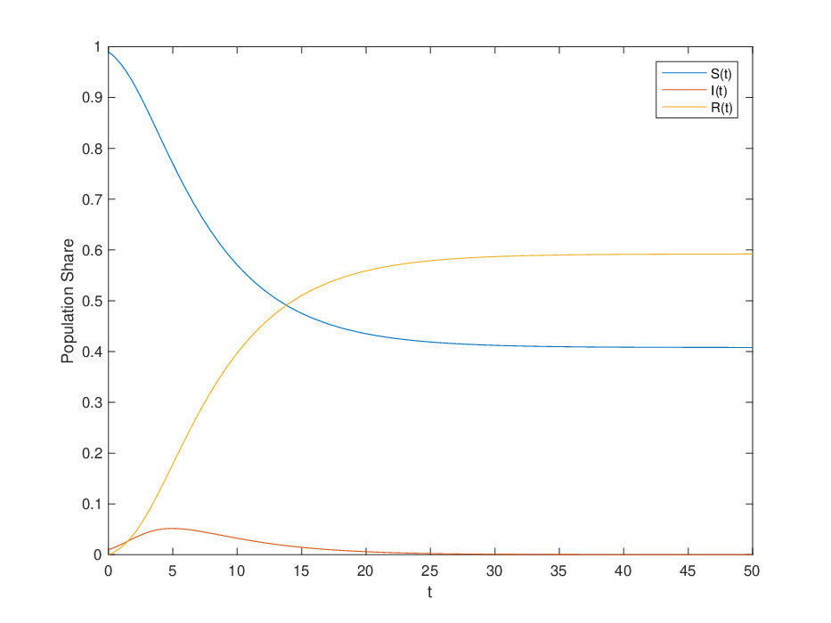
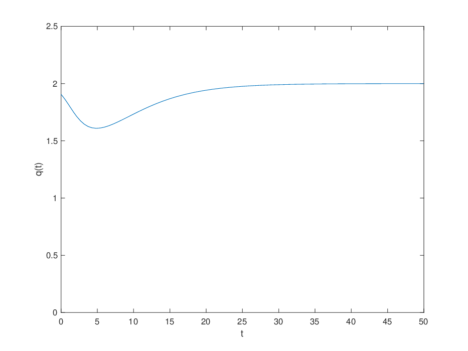
The proposition says that as long as the infected population is not larger than the susceptible population, the prevalence of the disease is single peaked. Figure 1 shows the path of the disease and behavior in a simple example.

If the population infected $I(t)$ is much larger than the population infected $S(t)$, then the prevalence may increase again late in the epidemic. The intuition is that in this case, most individuals who have not yet recovered are unlikely to be susceptible. Shifting some individuals from susceptible to infected would further decrease the chance of being susceptible. This mitigates infection risk and leads to more interaction (see Section 4 for similar effects). The proof gives a necessary condition for this to increase disease prevalence, which requires $I(t)>S(t)$ but is actually substantially stronger. This effect seems unlikely to occur in practice, as it would require unusually large prevalences for a severe disease and relies heavily on purely self-interested behavior.

We can also state single-peakedness results in terms of exogenous parameters, such as the transmission rate.

Corollary 1.

Let

$$(S(0),I(0),R(0))=(1-\epsilon,\epsilon,0).$$

If $C\beta>0$ is sufficiently small or $C\beta$ is sufficiently large, then the prevalence $I(t)$ is single-peaked for $\epsilon>0$ sufficiently small.

The threshold levels of $C\beta$ may depend on $a$ and $\kappa$. Similar single-peakedness results also hold for others parameters, i.e., when $a$ or $\kappa$ are sufficiently large.

When $I(t)$ is single-peaked, we can ask how exogenous shocks to the number of infected or recovered individuals affect the eventual fraction of the population $R(\infty)$ who has had the disease. To see this, it is useful to plot the curve $(I(t),R(t))\subset\mathbb{R}^{2}$. Shifting some susceptible individuals to infected will always shift this curve up, and therefore increase $R(\infty)$. Shifting some susceptible individuals to recovered will shift this curve right, which decreases $R(\infty)$ before the peak prevalence is reached and increases $R(\infty)$ after peak prevalence.

To state these observations formally, we consider a baseline time path $(S(t),I(t),R(t))$ as well as a modified time path $(\widetilde{S}(t),\widetilde{I}(t),\widetilde{R}(t))$ which includes an exogenous shock at time $t_{0}$, but otherwise follows equilibrium dynamics.

Proposition 3.

Suppose $I(t)$ is single-peaked. If

$$(\widetilde{S}(t_{0}),\widetilde{I}(t_{0}),\widetilde{R}(t_{0}))=(S(t_{0})-x,I(t_{0})+x,R(t_{0})),$$

then $\frac{\partial\widetilde{R}(\infty)}{\partial x}(0)\geq 0$. If

$$(\widetilde{S}(t_{0}),\widetilde{I}(t_{0}),\widetilde{R}(t_{0}))=(S(t_{0})-x,I(t_{0}),R(t_{0})+x),$$

then $\frac{\partial\widetilde{R}(\infty)}{\partial x}(0)\leq 0$ when $\dot{I}(t_{0})>0$ and $\frac{\partial\widetilde{R}(\infty)}{\partial x}(0)\geq 0$ when $\dot{I}(t_{0})<0$.

Numerical examples suggest, however, that marginal changes in the initial population have relatively small effects $R(\infty)$. So in our model, temporary policy changes early in an epidemic or even near the peak change the eventual fraction of the population effected, but the effect size may not be very large. This has several caveats in practice, e.g., the possibility of eradicating a disease or the arrival of a vaccine.

Figure 2: Recovered population over time for $C=0$ (blue), $C=1$ (red), and $C=5$ (yellow), with $a=\frac{1}{4}$, $\beta=\frac{1}{2},$ and $\kappa=1$.

By contrast, changes in $C$ lead to large differences in $R(\infty)$. For example, let $a=\frac{1}{4}$, $\beta=\frac{1}{2},$ and $\kappa=1$ and consider a small initial infection. The eventual fraction infected $R(\infty)$ is $80\%$ with $C=0$ but drops to $72\%$ with $C=1$ and just $59\%$ with $C=5$ (see Figure 2).

4 Risk Compensation

We next identify a region in which counterintuitive comparative statics occur because increases in infection risk lead to large changes in behavior. We find that a single condition determines the short-run impacts of changes in infection risk along a number of dimensions.

Definition 2.

We say that there are strong behavioral responses at time $t$ if

$$C\beta\cdot\frac{S(t)I(t)}{I(t)+S(t)}>2a.$$ (2)

Strong behavioral responses require a high cost of infection and large populations of susceptible and infected individuals. We will see that behavioral responses to policies is most important when these conditions hold. Note that these two conditions can work against each other, as individuals will interact less in response to costly infections, so such a region will only exist for diseases that are severe and highly infectious.

4.1 Increased Prevalence

The first consequence of strong behavioral responses is that infection rates are decreasing in disease prevalence, holding the recovered population fixed. Formally:

Proposition 4.

Let $(S_{x}(t),I_{x}(t),R_{x}(t))=(S(t)-x,I(t)+x,R(t))$ and let $\iota_{x}(t)$ be the corresponding infection rate. If $I(t)<S(t)$, then

$$\frac{\partial\iota_{x}(t)}{\partial x}(0)<0.$$

if and only if there are strong behavioral responses at time $t$.

During severe outbreaks, a larger number of individuals infected near the peak can lead to more social distancing. The proposition says that this could be large enough to decrease infection rate.

The proof shows that

$$\frac{\partial\iota_{x}(t)}{\partial x}(0)=\frac{S(t)-I(t)}{(2a+C\beta\frac{S(t)I(t)}{I(t)+S(t)})^{2}}\cdot(\underbrace{2a}_{\text{direct effect}}-\underbrace{C\beta\frac{S(t)I(t)}{S(t)+I(t)}}_{\text{behavioral effect}}).$$

Increasing the disease prevalence has two effects. First, the positive term corresponds to the direct effect of the change in the infection rate holding behavior fixed, which is positive whenever $I(t)<S(t)$. But second, the negative term corresponds to the effects of the change in behavior in response to the increased infection. A higher prevalence leads to a lower level of activity $q(t)$ (when $I(t)<S(t)$), which lowers the infection rate. Condition (2) determines whether the behavioral effect is larger than the direct effect. By contrast, the standard SIR model only captures the direct effect.

Figure 3: Time path of $I(t)$ in blue and $2a-C\beta\cdot\frac{S(t)I(t)}{I(t)+S(t)}$ (red), with $a=\frac{1}{10}$, $C=10$, $\beta=\frac{1}{2},$ and $\kappa=1$. There are strong behavioral responses if and only if the red curve is below zero.

Figure 3 gives an example with $a=\frac{1}{10}$, $C=10$, $\beta=\frac{1}{2},$ and $\kappa=1$. The infection path is shown in blue, and there are strong behavioral responses when the red curve is negative.

4.2 Policy

We next consider comparative in the cost $C$ from infection and the transmission rate $\beta$, which correspond to public-health measures that change the spread of the disease. Our strong behavioral responses condition again gives the impact of these policies.

Proposition 5.

The following are equivalent:

1. There are strong behavioral responses at time $t$,

2. Marginally decreasing $\beta$ at time $t$ increases $\iota(t)$, and

3. Marginally decreasing $C$ at time $t$ increases $C\iota(t)$.

An example of a policy to decrease $\beta$ is recommending or requiring individuals where masks. An example of a policy to decrease $C$ is developing a partially effective treatment. The proposition says that these policies increase short-term infection rates in the same region, which is characterized by high prevalence and a high cost of infection. Formally, (2) and (3) state the derivatives

$$\frac{\partial\iota(t)}{\partial\beta}<0\text{ and }\frac{\partial(C\iota(t))}{\partial C}<0$$

at the initial values of $\beta$ and $C$.

The model suggests that considering behavioral responses to public health policies is most important for severe diseases and close to the peak of outbreaks. When prevalence is low, public health interventions are most effective on their own. Near the peak, these interventions will tend to be less effective or even counterproductive unless paired with campaigns or restrictions to encourage social distancing.

Related models find that partially effective vaccines can increase infection rates (Kremer, 1996) and even decrease welfare (Talamas and Vohra, 2020). We consider these effects in a dynamic model and obtain a simple expression for when during the course of an outbreak this would occur.

Appendix A Proofs

Proof of Proposition 1.

We first show that $I(t)\rightarrow 0$. If not, we could choose $\epsilon>0$ and a sequence $t_{1},t_{2},\ldots$ such that $t_{i+1}>t_{i}+1$ and $I(t_{i})>\epsilon$. Because infected individuals recover at a Poisson rate $\kappa$, there exists $\delta>0$ such that if $I(t)>\epsilon$, at least $\delta$ individuals recover in the time interval $[t,t+1]$. Thus at least $\delta$ individuals recover in perod $[t_{i},t_{i}+1]$ for each $i$, which gives a contradiction since there is a unit mass of agents who can recover at most once each.

Let $R(\infty)=\lim_{t\rightarrow\infty}R(t)$. We next show that $R(\infty)\in(0,1)$. Because $I(0)>0$ and infected individuals recover at a Poisson rate, $R(\infty)>0$.

Suppose that $R(\infty)=1$, so that $S(t)\rightarrow 0$. Because $q(t)\leq\overline{q}$ for all $t$, we can bound $R(\infty)$ above by the limit of $R(t)$ when all individuals choose activity $q(t)=\overline{q}$ for all $t$:

Lemma 1.

Let $\overline{R}(t)$ be the share of recovered individuals when all individuals choose level of activity $\overline{q}$ for all $t$. Then $R(\infty)\leq\overline{R}(\infty)$.

Proof.

Define an infection chain $i_{0},\ldots,i_{k}$ of length $k$ to be a sequence of $k$ individuals such that $i_{0}$ is infected at time zero and for each $0\leq j<k$, individual $i_{j}$ meets individual $i_{j+1}$ while individual $i_{j}$ is infected. Then $R(\infty)$ is equal to the share of agents who are in an infection chain of length $k$ for any $k$. So it is sufficient to show that the number of individuals in infection chain of length $k$ for any $k$ is weakly higher under level of activity $\overline{q}$ at all times compared to $q(t)$.

We claim that for each $k$, the share of individuals in infection chains of length at most $k$ is weakly higher under actions $\overline{q}$ at all times compared to $q(t)$. The proof of the claim is by induction, and when $k=0$ the share is $I(0)$ in both cases.

Suppose the claim holds for $k$. Consider some individual $i$ who is not in an infection chain of length at most $k$. Then $i$ is in an infection chain of length $k+1$ if and only if $i$ meets at least one individual in an infection chain of length at most $k$ while that individual is infected. By the inductive hypothesis, there are weakly more individuals in an infection chain of length at most $k$ under actions $\overline{q}$ at all times compared to $q(t)$. As meetings are independent, the probability of meeting any such individual is increasing in $q_{i}(t)$ and $q_{I}(t)$ for all $t$. So the probability that $i$ is in an infection chain of length $k+1$ is weakly higher under actions $\overline{q}$ at all times compared to $q(t)$. Therefore, the claim holds for $k+1$. This completes the induction and therefore proves the lemma. ∎

By the lemma, we can assume for the remainder of the argument that $q(t)=\overline{q}$ for all $t$. We then have infection rate $S(t)I(t)\overline{q}^{2}\beta$ and recovery rate $\kappa I(t)$.

We claim that $\frac{S(t)}{I(t)}\rightarrow\infty$. Because $S(t)\rightarrow 0$ and $I(t)\rightarrow 0$, we can choose at time $t_{0}$ such that $\frac{S(t)\overline{q}^{2}\beta}{\kappa}\leq\frac{1}{4}$ and $\frac{I(t)\overline{q}^{2}\beta}{\kappa}\leq\frac{1}{4}$ for all $t\geq t_{0}$. Then for all $t\geq t_{0}$, we have $\dot{S}(t)\geq-\frac{\kappa}{4}S(t)$ by the first inequality and $\dot{I}(t)\leq-\frac{\kappa}{2}I(t)$ by the second inequality. In particular, $I(t)$ exponentially decays at a faster rate than $S(t)$. Since $S(t_{0})$ and $I(t_{0})$ are positive, this proves the claim.

We can therefore choose $t_{1}$ such that $S(t)>I(t)$ for all $t\geq t_{1}$ and $S(t)I(t)\overline{q}^{2}\beta<\frac{1}{2\kappa}$ for all $t\geq t_{1}$. Given an individual $i$ who is infected at time $t\geq t_{0}$, the second inequality implies that the expected number of susceptible individuals whom $i$ infects is less than $\frac{1}{2}$. Therefore, the total number of individuals who become infected at times $t\geq t_{0}$ is less than

$$I(t_{0})\sum_{k=1}^{\infty}\frac{1}{2^{k}}=I(t_{0})<S(t_{0}).$$

This contradicts our assumption that $S(t)\rightarrow 0$, so we must have $R(\infty)<1$. ∎

Proof of Proposition 2.

The population shares $(S(t),I(t),R(t))$ and $q(t)$ are continuous, so $\dot{I}(t)$ is continuous as well.

We first show that for $\epsilon$ sufficiently small, $\dot{I}(0)>0$. By Assumption 1 (high transmissivity), $\overline{q}^{2}\beta>\kappa$. Because $q(0)$ is a continuous function of $(S(t),I(t),R(t))$ with $q(0)=\overline{q}$ when $I(t)=0$, it follows that

$$(1-\epsilon)q(0)^{2}\beta>\kappa$$

for $\epsilon>0$ sufficiently small. Since $\dot{I}(0)=\epsilon(1-\epsilon)q(0)^{2}\beta-\epsilon\kappa$, the prevalence is initially increasing for $\epsilon$ sufficiently small.

Let $t^{peak}$ be the first time at which $\dot{I}(t)=0$. We will show that $\dot{I}(t)<0$ on $(t^{peak},t^{*})$ whenever $S(t)>I(t)$ on $(t^{peak},t^{*})$.

We first claim that $\ddot{I}(t^{peak})<0$. Let

$$(S(t),I(t),R(t))=(S(t^{peak})-x,I(t^{peak}),R(t^{peak})+x).$$

The infection rate is $\iota(t)=q(t)^{2}S(t)I(t)\beta$, and from equation (1)

$$q(t)=\frac{1}{2a+C\beta\cdot\frac{I(t)S(t)}{S(t)+I(t)}}\Rightarrow\frac{\partial q(t)}{\partial x}=-\frac{1}{(2a+C\beta\cdot\frac{I(t)S(t)}{S(t)+I(t)})^{2}}\cdot\frac{I(t)^{2}}{(S(t)+I(t))^{2}}.$$

So the derivative of the infection rate in $x$ is

$$\frac{\partial\iota(t)}{\partial x} =q(t)\beta I(t)\left(q(t)+2\frac{\partial q(t)}{\partial x}S(t)\right)$$

$$=\frac{q(t)\beta I(t)}{(2a+C\beta\cdot\frac{S(t)I(t)}{S(t)+I(t)})^{2}}\left(\left(2a+C\beta\cdot\frac{S(t)I(t)(S(t)+I(t))}{(S(t)+I(t))^{2}}\right)-2C\beta\cdot\frac{S(t)I(t)^{2}}{(S(t)+I(t))^{2}}\right)$$

$$=\frac{q(t)\beta I(t)}{(2a+C\beta\cdot\frac{S(t)I(t)}{S(t)+I(t)})^{2}}\left(2a+C\beta\cdot\frac{S(t)}{(S(t)+I(t))^{2}}\cdot(S(t)-I(t))\right).$$

We will need that the right-hand side is positive, which holds whenever $S(t)>I(t)$.

Since $\dot{I}(t^{peak})=0$ while $\dot{S}(t^{peak})=-\dot{R}(t^{peak})=\iota(t^{peak}),$ the derivative above implies that the derivative of the infection rate $\dot{\iota}(t^{peak})<0$. Since the time derivative of the recovery rate is $\kappa\dot{I}(t^{peak})=0$, the claim $\ddot{I}(t^{peak})<0$ holds.

Similarly, suppose that $\dot{I}(t)=0$ for some $t\in(t^{peak},t^{*})$. The same argument shows that $\ddot{I}(t)<0$ at time $t$. So $I(t)$ is strictly decreasing on $[t^{peak},t^{*}]$. ∎

Proof of Corollary 1.

We treat the two cases of $C\beta$ small and $C\beta$ large separately.

$C\beta$ small: By the proof of Proposition 2, $I(t)$ is single-peaked if $\epsilon$ is sufficiently small and

$$2a+C\beta\cdot\frac{S(t)}{(S(t)+I(t))^{2}}\cdot(S(t)-I(t))>0$$

for all $t$.

We claim the expression $-\frac{S(t)I(t)}{(S(t)+I(t))^{2}}$ is bounded below by a constant $M$ independent of $C$ and $\beta$ (but potentially depending on $a$ and $\kappa$). Indeed, $S(t)I(t)$ is bounded above by one. The expression $S(t)+I(t)$ is bounded below by the value of $1-R(\infty)$ when $\beta=1$ and $C=0$, so that $q(t)=\overline{q}$ for all $t$ (Lemma 1). Since $1-R(\infty)>0$ by Proposition 1, this proves the claim.

We conclude that whenever $C\beta<\frac{2a}{M},$ the prevalence $I(t)$ is single-peaked for $\epsilon$ sufficiently small.

$C\beta$ large: We next consider $C\beta$ large, and will show that for any $C\beta$ sufficiently large, we have $I(t)<S(t)$ for all $t$ when $\epsilon$ is small enough. As above, we can bound $1-R(\infty)$ below by a positive constant, which we call $N$.

Let $\delta<N/2$. We will show that for $C\beta$ sufficiently large and $\epsilon<\delta/2$, we have $I(t)<\delta$ for all $t$. If not, there must exist some time $t_{0}$ at which $\delta/2<I(t_{0})<\delta$ and $\dot{I}(t_{0})>0$.

Since $I(t_{0})+S(t_{0})\geq N$, $I(t_{0})<\delta$, and $\delta<N/2$, we have $S(t_{0})>I(t_{0})$. Therefore, $\frac{I(t_{0})S(t_{0})}{S(t_{0})+I(t_{0})}\geq\frac{I(t_{0})}{2}\geq\frac{\delta}{4}$. Recall that $q(t)=\frac{1}{2a+C\beta\cdot\frac{I(t)S(t)}{S(t)+I(t)}}$. So taking $C\beta$ sufficiently large, we can assume that $q(t_{0})<\sqrt{\kappa}$. Then

$$\dot{I}(t_{0})=I(t_{0})\left(\frac{S(t_{0})}{I(t_{0})+S(t_{0})}q(t_{0})^{2}\beta-\kappa\right)\leq I(t_{0})(q(t_{0})^{2}-\kappa)<0.$$

But this contradicts our assumption that $\dot{I}(t_{0})>0$.

We have shown $I(t)<\delta$ for all $t$. Since $I(t)+S(t)\geq N>2\delta$ for all $t$, we must have $I(t)<S(t)$ for all $t$ as desired. We now apply Proposition 2. ∎

Proof of Proposition 3.

We compare the curves $(I(t),R(t))$ and $(\widetilde{I}(t),\widetilde{R}(t))$ in $\mathbb{R}^{2}$. For each comparative static, there will be two cases depending on whether these curves intersect after the shock.

To carry out this comparison, we first note that the function $R(t)$ is continuous and strictly increasing with image $[R(0),R(\infty))$. So for each $r\in[R(0),R(\infty)),$ the inverse $R^{-1}(r)$ is unique.

Consider a shock at time $t_{0}$. First, let $(\widetilde{S}(t_{0}),\widetilde{I}(t_{0}),\widetilde{R}(t_{0}))=(S(t_{0})-x,I(t_{0})+x,R(t_{0}))$ for $x>0$. For each $r\in[R(t_{0}),R(\infty))$, the inverse $R^{-1}(r)$ is the time at which $R(t)=r$. We can compare $I(R^{-1}(r))$ to $\widetilde{I}(\widetilde{R}^{-1}(r))$. Since $\widetilde{I}(t_{0})>I(t_{0})$, we either have $I(R^{-1}(r))=\widetilde{I}(\widetilde{R}^{-1}(r))$ for some $r>R(t_{0})$ or $I(R^{-1}(r))>\widetilde{I}(\widetilde{R}^{-1}(r))$ for all $r\in[R(t_{0}),R(\infty))$.

If $I(R^{-1}(r))=\widetilde{I}(\widetilde{R}^{-1}(r))$ for some $r>R(t_{0})$, then the dynamics of $(\widetilde{S}(t),\widetilde{I}(t),\widetilde{R}(t))$ beginning at time $\widetilde{R}^{-1}(r)$ are the same as the dynamics of $(S(t),I(t),R(t))$ beginning at time $R^{-1}(r)$, so $\widetilde{R}(\infty)=R(\infty)$. If $I(R^{-1}(r))>\widetilde{I}(\widetilde{R}^{-1}(r))$ for all $r\in[R(t_{0}),R(\infty))$, then $\widetilde{R}(\infty)\geq R(\infty)$ by continuity of $R(t)$.

Next, let $(\widetilde{S}(t_{0}),\widetilde{I}(t_{0}),\widetilde{R}(t_{0}))=(S(t_{0})-x,I(t_{0}),R(t_{0})+x)$ for $x>0$ arbitrarily small. There exists a time $t_{1}$ at which $R(t_{1}))=\widetilde{R}(t_{0}).$ If $\dot{I}(t_{0})>0$, then $\widetilde{I}(t_{0})<I(t_{1})$. So we either have $I(R^{-1}(r))=\widetilde{I}(\widetilde{R}^{-1}(r))$ for some $r>R(t_{1})$ or $I(R^{-1}(r))<\widetilde{I}(\widetilde{R}^{-1}(r))$ for all $r\in[R(t_{1}),R(\infty))$. As in the previous paragraph, we can conclude that $\widetilde{R}(\infty)\leq R(\infty)$.

If $\dot{I}(t_{0})<0$, then $\widetilde{I}(t_{0})>I(t_{1})$. So we either have $I(R^{-1}(r))=\widetilde{I}(\widetilde{R}^{-1}(r))$ for some $r>R(t_{1})$ or $I(R^{-1}(r))>\widetilde{I}(\widetilde{R}^{-1}(r))$ for all $r\in[R(t_{1}),R(\infty))$. As in the previous cases, we can conclude that $\widetilde{R}(\infty)\geq R(\infty)$. ∎

Proof of Proposition 4.

Let $q_{x}(t)$ be the equilibrium action given $(S_{x}(t),I_{x}(t),R_{x}(t))$. The infection rate is $\iota_{x}(t)=q_{x}(t)^{2}S_{x}(t)I_{x}(t)\beta$, and from equation (1)

$$q_{x}(t)=\frac{1}{2a+C\beta\cdot\frac{I_{x}(t)S_{x}(t)}{S_{x}(t)+I_{x}(t)}}.$$

As $x$ varies, $S_{x}(t)+I_{x}(t)$ remains constant while $\frac{\partial\left(S_{x}(t)I_{x}(t)\right)}{\partial x}(0)=I(t)-S(t)$.

Differentiating the infection rate,

$$\frac{\partial\iota_{x}(t)}{\partial x}(0)=q(t)^{2}(I(t)-S(t))\beta+2q(t)\left(\frac{\partial q_{x}(t)}{\partial x}(0)\right)S(t)I(t)\beta.$$

The right-hand side has the same sign as $q(t)(I(t)-S(t))+2\left(\frac{\partial q_{x}(t)}{\partial x}(0)\right)S(t)I(t).$ Differentiating $q_{x}(t)$,

$$\left(\frac{\partial q_{x}(t)}{\partial x}(0)\right)=-\frac{C\beta\cdot\frac{I(t)-S(t)}{S(t)+I(t)}}{\left(2a+C\beta\cdot\frac{I(t)S(t)}{S(t)+I(t)}\right)^{2}}.$$

Substituting,

$$q(t)+2\left(\frac{\partial q_{x}(t)}{\partial x}(0)\right)\beta=\frac{I(t)-S(t)}{\left(2a+C\beta\cdot\frac{I(t)S(t)}{S(t)+I(t)}\right)^{2}}\cdot\left(2a-C\beta\cdot\frac{I(t)S(t)}{S(t)+I(t)}\right).$$

Suppose $I(t)<S(t)$. The right-hand side is negative if and only if $2a-C\beta\cdot\frac{I(t)S(t)}{S(t)+I(t)}<0$, which is the definition of a strong behavioral response at $t$. ∎

Proof of Proposition 5.

We will again use our formula for the infection rate $\iota(t)=q(t)^{2}S(t)I(t)\beta$ and equation (1) for $q(t)$.

(1) $\Leftrightarrow$ (2): Differentiating the infection rate,

$$\frac{\partial\iota(t)}{\partial\beta}=q(t)^{2}S(t)I(t)+2q(t)\frac{\partial q(t)}{\partial\beta}S(t)I(t)\beta.$$

The right-hand side has the same sign as $q(t)+2\frac{\partial q(t)}{\partial\beta}\beta.$ Differentiating $q(t)$,

$$\frac{\partial q(t)}{\partial\beta}=-\frac{C\beta\cdot\frac{I(t)S(t)}{S(t)+I(t)}}{\left(2a+C\beta\cdot\frac{I(t)S(t)}{S(t)+I(t)}\right)^{2}}.$$

Substituting,

$$q(t)+2\frac{\partial q(t)}{\partial\beta}\beta=\frac{1}{\left(2a+C\beta\cdot\frac{I(t)S(t)}{S(t)+I(t)}\right)^{2}}\cdot\left(2a-C\beta\cdot\frac{I(t)S(t)}{S(t)+I(t)}\right).$$

The right-hand side is negative if and only if $2a-C\beta\cdot\frac{I(t)S(t)}{S(t)+I(t)}<0$, which is the definition of a strong behavioral response at $t$.

(2) $\Leftrightarrow$ (3): Because $C$ is constant, the infection rate $\iota(t)$ is decreasing in $\beta$ if and only if $C\iota(t)$ is decreasing in $\beta$. In our expression for $C\iota(t)$, the terms $C$ and $\beta$ only within the product $C\beta$. So $C\iota(t)$ is decreasing in $\beta$ if and only if it is decreasing in $C$. ∎

References

- Auld (2003) Auld, M. C. (2003): “Choices, beliefs, and infectious disease dynamics,” Journal of Health Economics, 22, 361–377.
- Eichenbaum et al. (2020) Eichenbaum, M. S., S. Rebelo, and M. Trabandt (2020): “The macroeconomics of epidemics,” Working Paper.
- Farboodi et al. (2020) Farboodi, M., G. Jarosch, and R. Shimer (2020): “Internal and external effects of social distancing in a pandemics,” COVID Economics, 22–58.
- Fenichel et al. (2011) Fenichel, E. P., C. Castillo-Chavez, M. G. Ceddia, G. Chowell, P. A. G. Parra, G. J. Hickling, G. Holloway, R. Horan, B. Morin, C. Perrings, et al. (2011): “Adaptive human behavior in epidemiological models,” Proceedings of the National Academy of Sciences, 108, 6306–6311.
- Ferguson et al. (2020) Ferguson, N., D. Laydon, G. Nedjati Gilani, N. Imai, K. Ainslie, M. Baguelin, S. Bhatia, A. Boonyasiri, Z. Cucunuba Perez, G. Cuomo-Dannenburg, et al. (2020): “Report 9: Impact of non-pharmaceutical interventions (NPIs) to reduce COVID19 mortality and healthcare demand,” Working Paper.
- Funk et al. (2015) Funk, S., S. Bansal, C. T. Bauch, K. T. Eames, W. J. Edmunds, A. P. Galvani, and P. Klepac (2015): “Nine challenges in incorporating the dynamics of behaviour in infectious diseases models,” Epidemics, 10, 21–25.
- Greenwood et al. (2019) Greenwood, J., P. Kircher, C. Santos, and M. Tertilt (2019): “An equilibrium model of the African HIV/AIDS epidemic,” Econometrica, 87, 1081–1113.
- Kissler et al. (2020) Kissler, S. M., C. Tedijanto, E. Goldstein, Y. H. Grad, and M. Lipsitch (2020): “Projecting the transmission dynamics of SARS-CoV-2 through the postpandemic period,” Science.
- Korinek and Bethune (2020) Korinek, A. and Z. Bethune (2020): “COVID-19 Infection Externalities: Trading Off Lives vs. Livelihoods,” Working Paper.
- Kremer (1996) Kremer, M. (1996): “Integrating behavioral choice into epidemiological models of AIDS,” The Quarterly Journal of Economics, 111, 549–573.
- Kruger et al. (2020) Kruger, D., H. Uhlig, and T. Xie (2020): “Macroeconomic Dynamics and Reallocation in an Epidemic,” University of Chicago, Becker Friedman Institute for Economics Working Paper.
- Manfredi and D’Onofrio (2013) Manfredi, P. and A. D’Onofrio (2013): Modeling the interplay between human behavior and the spread of infectious diseases, Springer Science & Business Media.
- Talamas and Vohra (2020) Talamas, E. and R. Vohra (2020): “Go big or go home: a free and perfectly safe but only partially effective vaccine can make everyone worse off,” Games and Economic Behavior.