Pushing the Envelope: From Discrete to Continuous Movements in Multi-Agent Path Finding via Lazy Encodings

Abstract

Multi-agent path finding in continuous space and time with geometric agents MAPF^R is addressed in this paper. The task is to navigate agents that move smoothly between predefined positions to their individual goals so that they do not collide. We introduce a novel solving approach for obtaining makespan optimal solutions called SMT-CBS^R based on satisfiability modulo theories (SMT). The new algorithm combines collision resolution known from conflict-based search (CBS) with previous generation of incomplete SAT encodings on top of a novel scheme for selecting decision variables in a potentially uncountable search space. We experimentally compare SMT-CBS^R and previous CCBS algorithm for MAPF^R.

1 Introduction

In multi-agent path finding (MAPF) [15, 27, 24, 30, 40, 26, 25, 6] the task is to navigate agents from given starting positions to given individual goals. The problem takes place in undirected graph $G=(V,E)$ where agents from set $A=\{a_{1},a_{2},...,a_{k}\}$ are placed in vertices with at most one agent per vertex. The initial configuration can be written as $\alpha_{0}:A\rightarrow V$ and similarly the goal configuration as $\alpha_{+}:A\rightarrow V$. The task of navigating agents can be then expressed formally as transforming $\alpha_{0}$ into $\alpha_{+}$ while movements are instantaneous and are possible across edges assuming no other agent is entering the same target vertex in the standard MAPF.

In order to reflect various aspects of real-life applications, variants of MAPF have been introduced such as those considering kinematic constraints [9], large agents [17], generalized costs of actions [39], or deadlines [19] - see [18, 28] for more variants. Particularly in this work we are dealing with an extension of MAPF introduced only recently [1, 36] that considers continuous time and space (MAPF^R) where agents move smoothly along predefined curves interconnecting predefined positions placed arbitrarily in some continuous space. It is natural in MAPF^R to assume geometric agents of various shapes that occupy certain volume in the space - circles in the 2D space, polygons, spheres in the 3D space etc. In contrast to MAPF, where the collision is defined as the simultaneous occupation of a vertex or an edge by two agents, collisions are defined as any spatial overlap of agents’ bodies in MAPF^R.

The motivation behind introducing MAPF^R is the need to construct more realistic paths in many applications such as controlling fleets of robots or aerial drones [10, 7] where continuous reasoning is closer to the reality than the standard MAPF.

We contribute by showing how to apply satisfiability modulo theory (SMT) reasoning [5, 20] in makespan optimal MAPF^R solving. Particularly we extend the preliminary work in this direction from [34, 33, 36]. The SMT paradigm constructs decision procedures for various complex logic theories by decomposing the decision problem into the propositional part having arbitrary Boolean structure and the complex theory part that is restricted on the conjunctive fragment. Our SMT-based algorithm called SMT-CBS^R combines the Conflict-based Search (CBS) algorithm [25, 8] with previous algorithms for solving the standard MAPF using incomplete encodings [35, 32, 31] and continuous reasoning.

1.1 Related Work and Organization

Using reductions of planning problems to propositional satisfiability has been coined in the SATPlan algorithm and its variants [12, 13, 14, 11]. Here we are trying to apply similar idea in the context of MAPF^R. So far MAPF^R has been solved by a modified version of CBS that tries to solve MAPF lazily by adding collision avoidance constraints on demand. The adaptation of CBS for MAPF^R consists in implementing continuous collision detection while the high-level framework of the algorithm remains the same as demonstrated in the CCBS algorithm [1].

We follow the idea of CBS too but instead of searching the tree of possible collision eliminations at the high-level we encode the requirement of having collision free paths as a propositional formula [4] and leave it to the SAT solver as done in [37]. We construct the formula lazily by adding collision elimination refinements following [35] where the lazy construction of incomplete encodings has been suggested for the standard MAPF within the algorithm called SMT-CBS. SMT-CBS works with propositional variables indexed by agent $a$, vertex $v$, and time step $t$ with the meaning that if the variable is $\mathit{TRUE}$ $a$ in $v$ at time step $t$. In MAPF^R we however face major technical difficulty that we do not know necessary decision (propositional) variables in advance and due to continuous time we cannot enumerate them all as in the standard MAPF. Hence we need to select from a potentially uncountable space those variables that are sufficient for finding the makespan optimal solution.

The organization is as follows: we first introduce MAPF^R. Then we recall CCBS, a variant of CBS for MAPF^R. Details of the novel SMT-based solving algorithm SMT-CBS^R follow. Finally, a comparison SMT-CBS^R with CCBS is shown.

1.2 MAPF in Continuous Time and Space

We use the definition of MAPF in continuous time and space denoted MAPF^R from [39] and [1]. MAPF^R shares components with the standard MAPF: undirected graph $G=(V,E)$, set of agents $A=\{a_{1},a_{2},...,a_{k}\}$, and the initial and goal configuration of agents: $\alpha_{0}:A\rightarrow V$ and $\alpha_{+}:A\rightarrow V$. A simple 2D variant of MAPF^R is as follows:

Definition 1

(MAPF^R) Multi-agent path finding with continuous time and space (MAPF^R) is a 5-tuple $\Sigma^{\mathcal{R}}=(G=(V,E),A,\alpha_{0},\alpha_{+},\rho)$ where $G$, $A$, $\alpha_{0}$, $\alpha_{+}$ are from the standard MAPF and $\rho$ determines continuous extensions:

• $\rho.x(v),\rho.y(v)$ for $v\in V$ represent the position of vertex $v$ in the 2D plane

• $\rho.speed(a)$ for $a\in A$ determines constant speed of agent $a$

• $\rho.radius(a)$ for $a\in A$ determines the radius of agent $a$; we assume that agents are circular discs with omni-directional ability of movements

We assume that agents have constant speed and instant acceleration. The major difference from the standard MAPF where agents move instantly between vertices (disappears in the source and appears in the target instantly) is that smooth continuous movement between a pair of vertices (positions) along the straight line interconnecting them takes place in MAPF^R. Hence we need to be aware of the presence of agents at some point in the 2D plane at any time.

Figure 1: An example of MAPF^R instance with two agents. A feasible makespan sub-optimal solution $\pi$ (makespan $\mu(\pi)=2.0$) and makespan optimal solution $\pi*$ (makespan $\mu(\pi*)=1.980$) are shown.

Collisions may occur between agents in MAPF^R due to their volume; that is, they collide whenever their bodies overlap. In contrast to MAPF, collisions in MAPF^R may occur not only in a single vertex or edge being shared by colliding agents but also on pairs of edges (lines interconnecting vertices) that are too close to each other and simultaneously traversed by large agents.

We can further extend the continuous properties by introducing the direction of agents and the need to rotate agents towards the target vertex before they start to move. Also agents can be of various shapes not only circular discs [17] and can move along various fixed curves.

For simplicity we elaborate our implementations for the above simple 2D continuous extension with circular agents. We however note that all developed concepts can be adapted for MAPF with more continuous extensions.

A solution to given MAPF^R $\Sigma^{\mathcal{R}}$ is a collection of temporal plans for individual agents $\pi=[\pi(a_{1}),$ $\pi(a_{2}),...,$ $\pi(a_{k})]$ that are mutually collision-free. A temporal plan for agent $a\in A$ is a sequence $\pi(a)=[((\alpha_{0}(a),\alpha_{1}(a)),$ $[t_{0}(a),t_{1}(a)));$ $((\alpha_{1}(a),\alpha_{2}(a)),$ $[t_{1}(a),t_{2}(a)));$ …; $((\alpha_{m(a)-1},\alpha_{m(a)}(a)),$ $[t_{m(a)-1},t_{m(a)}))]$ where $m(a)$ is the length of individual temporal plan and each pair $(\alpha_{i}(a),\alpha_{i+1}(a)),$ $[t_{i}(a),t_{i+1}(a)))$ corresponds to traversal event between a pair of vertices $\alpha_{i}(a)$ and $\alpha_{i+1}(a)$ starting at time $t_{i}(a)$ and finished at $t_{i+1}(a)$.

It holds that $t_{i}(a)<t_{i+1}(a)$ for $i=0,1,...,m(a)-1$. Moreover consecutive events in the individual temporal plan must correspond to edge traversals or waiting actions, that is: $\{\alpha_{i}(a),$ $\alpha_{i+1}(a)\}\in E$ or $\alpha_{i}(a)=\alpha_{i+1}(a)$; and times must reflect the speed of agents for non-wait actions.

The duration of individual temporal plan $\pi(a)$ is called an individual makespan; denoted $\mu(\pi(a))=t_{m(a)}$. The overall makespan of $\pi$ is defined as max${}_{i=1}^{k}(\mu(\pi(a_{i})))$. We focus on finding makespan optimal solutions. An example of MAPF^R and makespan optimal solution is shown in Figure 1.

Through straightforward reduction of MAPF to MAPF^R it can be observed that finding a makespan optimal solution with continuous time is an NP-hard problem [22, 41].

2 Solving MAPF with Continuous Time

Let us recall CCBS [1], a variant of CBS [25] modified for MAPF^R. The idea of CBS algorithms is to resolve conflicts lazily. CBS algorithms are usually developed for the sum-of-costs [26] objective but using other cumulative costs like makespan is possible too.

2.1 Conflict-based Search

CCBS for finding the makespan optimal solution is shown in Algorithm 1. The high-level of CCBS searches a constraint tree (CT) using a priority queue ordered according to the makespan in the breadth first manner. CT is a binary tree where each node $N$ contains a set of collision avoidance constraints $N.cons$ - a set of triples $(a_{i},(u,v),[t_{0},t_{+}))$ forbidding agent $a_{i}$ to start smooth traversal of edge $\{u,v\}$ (line) at any time between $[t_{0},t_{+})$, a solution $N.\pi$ - a set of $k$ individual temporal plans, and the makespan $N.\mu$ of $N.\pi$.

Algorithm 1 CCBS algorithm for solving MAPF^R.

1 CBS^R ($\Sigma^{\mathcal{R}}=(G=(V,E),A,\alpha_{0},\alpha_{+},\rho)$)

      2 $R.cons\leftarrow\emptyset$

      3 $R.\pi\leftarrow$ $\{$shortest temporal plan from $\alpha_{0}(a_{i})$ to $\alpha_{+}(a_{i})\;|\;i=1,2,...,k\}$

      4 $R.\mu\leftarrow\max_{i=1}^{k}{\mu(N.\pi(a_{i}))}$

      5 $\textsc{Open}\leftarrow\emptyset$

      6 insert $R$ into Open

      7 while $\textsc{Open}\neq\emptyset$ do

           8 $N\leftarrow$ min${}_{\mu}(\textsc{Open}$)

           9 remove-Min${}_{\mu}(\textsc{Open}$)

           10 $collisions\leftarrow$ validate-Plans($N.\pi$)

           11 if $collisions=\emptyset$ then

                12 return $N.\pi$

           13 let $(m_{i}\times m_{j})\in collisions$ where $m_{i}=(a_{i},(u_{i},v_{i}),[t_{i}^{0},t_{i}^{+}))$ and $m_{j}=(a_{j},(u_{j},v_{j}),[t_{j}^{0},t_{j}^{+}))$

           14 $([\tau_{i}^{0},\tau_{i}^{+});[\tau_{j}^{0},\tau_{j}^{+}))\leftarrow$ resolve-Collision($m_{i}$,$m_{j}$)

           15 for each $m\in\{(m_{i},[\tau_{i}^{0},\tau_{i}^{+})),(m_{j},[\tau_{j}^{0},\tau_{j}^{+}))\}$ do

                16 let $((a,(u,v),[t_{0},t_{+})),[\tau_{0},\tau_{+}))=m$

                17 $N^{\prime}.cons\leftarrow N.cons\cup\{(a,(u,v),[\tau_{0},\tau_{+}))\}$

                18 $N^{\prime}.\pi\leftarrow N.\pi$

                19 update($a$, $N^{\prime}.\pi$, $N^{\prime}.cons$)

                20 $N^{\prime}.\mu\leftarrow\max_{i=1}^{k}\mu{(N^{\prime}.\pi(a_{i}))}$

                21 insert $N^{\prime}$ into Open

The low-level in CCBS associated with node $N$ searches for individual temporal plan with respect to set of constraints $N.cons$. For given agent $a_{i}$, this is the standard single source shortest path search from $\alpha_{0}(a_{i})$ to $\alpha_{+}(a_{i})$ that at time $t$ cannot start to traverse any $\{(u,v)\in E\;|\;(a_{i},(u,v),[t_{0},t_{+}))\in N.cons\wedge t\in[t_{0},t_{+})\}$. Various intelligent single source shortest path algorithms such as SIPP [21] can be used here.

CCBS stores nodes of CT into priority queue Open sorted according to the ascending makespan. At each step CBS takes node $N$ with the lowest makespan from Open and checks if $N.\pi$ represents non-colliding temporal plans. If there is no collision, the algorithms returns valid solution $N.\pi$. Otherwise the search branches by creating a new pair of nodes in CT - successors of $N$. Assume that a collision occurred between $a_{i}$ traversing $(u_{i},v_{i})$ during $[t_{i}^{0},t_{i}^{+})$ and $a_{j}$ traversing $(u_{j},v_{j})$ during $[t_{j}^{0},t_{j}^{+})$. This collision can be avoided if either agent $a_{i}$ or agent $a_{j}$ waits after the other agent passes. We can calculate for $a_{i}$ so called maximum unsafe interval $[\tau_{i}^{0},\tau_{i}^{+})$ such that whenever $a_{i}$ starts to traverse $(u_{i},v_{i})$ at some time $t\in[\tau_{i}^{0},\tau_{i}^{+})$ it ends up colliding with $a_{j}$ assuming $a_{j}$ did not try to avoid the collision. Hence $a_{i}$ should wait until $\tau_{i}^{+}$ to tightly avoid the collision with $a_{j}$. Similarly we can calculate maximum unsafe interval for $a_{j}$: $[\tau_{j}^{0},\tau_{j}^{+})$. These two options correspond to new successor nodes of $N$: $N_{1}$ and $N_{2}$ that inherit set of constraints from $N$ as follows: $N_{1}.cons=N.cons$ $\cup$ $\{(a_{i},(u_{i},v_{i}),$ $[\tau_{i}^{0},\tau_{i}^{+}))\}$ and $N_{2}.cons=N.cons$ $\cup$ $\{(a_{j},(u_{j},v_{j}),$ $[\tau_{j}^{0},\tau_{j}^{+}))\}$. $N_{1}.\pi$ and $N_{1}.\pi$ inherits plans from $N.\pi$ except those for agents $a_{i}$ and $a_{j}$ respectively that are recalculated with respect to the constraints. After this $N_{1}$ and $N_{2}$ are inserted into Open.

2.2 A Satisfiability Modulo Theory Approach

We will use for the specific case of CCBS the idea introduced in [35] that rephrases the algorithm as problem solving in satisfiability modulo theories (SMT) [5, 38]. The basic use of SMT divides the satisfiability problem in some complex theory $T$ into a propositional part that keeps the Boolean structure of the problem and a simplified procedure $\mathit{DECIDE_{T}}$ that decides fragment of $T$ restricted on conjunctive formulae. A general $T$-formula $\Gamma$ being decided for satisfiability is transformed to a propositional skeleton by replacing its atoms with propositional variables. The standard SAT solver then decides what variables should be assigned $\mathit{TRUE}$ in order to satisfy the skeleton - these variables tells what atoms hold in $\Gamma$. $\mathit{DECIDE_{T}}$ then checks if the conjunction of atoms assigned $\mathit{TRUE}$ is valid with respect to axioms of $T$. If so then satisfying assignment is returned. Otherwise a conflict from $\mathit{DECIDE_{T}}$ (often called a lemma) is reported back to the SAT solver and the skeleton is extended with new constraints resolving the conflict. More generally not only new constraints are added to resolve the conflict but also new atoms can be added to $\Gamma$.

$T$ will be represented by a theory with axioms describing movement rules of MAPF^R; a theory we will denote $T_{\mathit{MAPF}^{\mathcal{R}}}$. $\mathit{DECIDE}_{\mathit{MAPF}^{\mathcal{R}}}$ can be naturally represented by the plan validation procedure from CCBS (validate-Plans).

2.3 RDD: Real Decision Diagram

The important question when using the logic approach is what will be the decision variables. In the standard MAPF, time expansion of $G$ for every time step has been done resulting in a multi-value decision diagram (MDD) [37] representing possible positions of agents at any time step. Since MAPF^R is inherently continuous we cannot afford to consider every time moment but we need to restrict on important moments only.

Analogously to MDD, we introduce real decision diagram (RDD). RDD_i defines for agent $a_{i}$ its space-time positions and possible movements. Formally, $RDD_{i}$ is a directed graph $(X^{i},E^{i})$ where $X_{i}$ consists of pairs $(u,t)$ with $u\in V$ and $t\in\mathbb{R}_{0}^{+}$ is time and $E_{i}$ consists of directed edges of the form $((u,t_{u});(v,t_{v}))$. Edge $((u,t_{u});(v,t_{v}))$ correspond to agent’s movement from $u$ to $v$ started at $t_{u}$ and finished at $t_{v}$. Waiting in $u$ is possible by introducing edge $((u,t_{u});(v,t^{\prime}_{u}))$. Pair $(\alpha_{0}(a_{i}),0)\in X_{i}$ indicates start and $(\alpha_{+}(a_{i}),t)$ for some $t$ corresponds to reaching the goal position.

Algorithm 2 Building of RDD for MAPF^R

1 build-RDDs($\Sigma^{\mathcal{R}}$, $\mathit{cons}$, $\mu_{max}$)

      2 for $i=1,2,...,k$ do

           3 $X^{i}\leftarrow\emptyset$, $E^{i}\leftarrow\emptyset$, $\textsc{Open}\leftarrow\emptyset$

           4 insert $(\alpha_{0}(a_{i}),0)$ into Open

           5 $X^{i}\leftarrow X^{i}\cup\{(\alpha_{0}(a_{i}),0)\}$

           6 while $\textsc{Open}\neq\emptyset$ do

                7 $(u,t)\leftarrow$ min${}_{t}(\textsc{Open}$)

                8 remove-Min${}_{t}(\textsc{Open}$)

                9 if $t\leq\mu_{max}$ then

                     10 for each $v\;|\;\{u,v\}\in E$ do

                          11 $\Delta t\leftarrow dist(u,v)/v_{a_{i}}$

                          12 insert $(v,t+\Delta t)$ into Open

                          13 $X^{i}\leftarrow X^{i}\cup\{(v,t+\Delta t)\}$

                          14 $E^{i}\leftarrow E^{i}\cup\{[(u,t);(v,t+\Delta t)]\}$

                          15 for each $(a_{i},(u,v),[\tau^{0},\tau^{+}))\in\mathit{cons}$ do

                               16 if $t\geq\tau^{0}$ and $t<\tau^{+}$ then

                                    17 insert $(u,\tau_{+})$ into Open

                                    18 $X^{i}\leftarrow X^{i}\cup\{(u,\tau^{+})\}$

                                    19 $E^{i}\leftarrow E^{i}\cup\{[(u,t);(u,\tau^{+})]\}$

      20 return $[(X^{1},E^{1}),(X^{2},E^{2}),...,(X^{k},E^{k})]$

RDDs for individual agents are constructed with respect to collision avoidance constraints. If there is no collision avoidance constraint then RDD_i simply corresponds to a shortest temporal plan for agent $a_{i}$. But if a collision avoidance constraint is present, say $(a_{i},(u,v),[\tau_{0},\tau_{+}))$, and we are considering movement starting in $u$ at $t$ that interferes with the constraint, then we need to generate a node into RDD_i that allows agent to wait until the unsafe interval passes by, that is node $(u,\tau^{+})$ and edge $((u,\tau^{+});(u,\tau^{+}))$ are added.

The process of building RDDs is formalized in Algorithm 2. It performs breadth-first search (BFS). For each possible edge traversal the algorithm generates a successor node and corresponding edge (lines 12-15) but also considers all possible wait action w.r.t. interfering collision avoidance constraints (lines 17-20). As a result each constraint is treated as both present and absent. In other words, RDD_i represents union of all paths for agent $a_{i}$ examined in all branches of the corresponding CT. The stop condition is specified by the maximum makespan $\mu_{max}$ beyond which no more actions are performed. An example of RDDs is shown in Figure 2.

Figure 2: Real decision diagrams (RDDs) for agents $a_{1}$ and $a_{2}$ from MAPF^R from Figure 1. Decisions corresponding to shortest paths for agents $a_{1}$ and $a_{2}$ moving diagonally towards their goals are shown: $a_{1}:1\rightarrow 4$, $a_{2}:2\rightarrow 3$ (left). This however results in a collision whose resolution is either waiting for agent $a_{1}$ in vertex 1 from $0.000$ until $0.566$ or waiting for agent $a_{2}$ in vertex 2 from $0.000$ until $0.566$; reflected in the next RDDs (right). Mutex is depicted using dotted line connecting arcs form RDD₁ and RDD₂.

2.4 SAT Encoding from RDD

We introduce a decision variable for each node and edge $[RDD{{}_{1}},...,RDD{{}_{k}}]$; RDD${}_{i}=(X^{i},E^{i})$: we have variable $\mathcal{X}_{u}^{t}(a_{i})$ for each $(u,t)\in X^{i}$ and $\mathcal{E}_{u,v}^{t_{u},t_{v}}(a_{i})$ for each directed edge $((u,t_{u});(v,t_{v}))\in E^{i}$. The meaning of variables is that $\mathcal{X}_{u}^{t}(a_{i})$ is $\mathit{TRUE}$ if and only if agent $a_{i}$ appears in $u$ at time $t$ and similarly for edges: $\mathcal{E}_{u,v}^{t_{u},t_{v}}(a_{i})$ is $\mathit{TRUE}$ if and only if $a_{i}$ moves from $u$ to $v$ starting at time $t_{u}$ and finishing at $t_{v}$.

MAPF^R rules are encoded on top of these variables so that eventually we want to obtain formula $\mathcal{F}(\mu)$ that encodes existence of a solution of makespan $\mu$ to given MAPF^R. We need to encode that agents do not skip but move along edges, do not disappear or appear from nowhere etc. We show below constraints stating that if agent $a_{i}$ appears in vertex $u$ at time step $t_{u}$ then it has to leave through exactly one edge connected to $u$ (constraint (2) although Pseudo-Boolean can be encoded using purely propositional means):

$${\mathcal{X}_{u}^{t_{u}}(a_{i})\Rightarrow\bigvee_{(v,t_{v})\;|\;((u,t_{u}),(v,t_{v}))\in E^{i}}{\mathcal{E}^{t_{u},t_{v}}_{u,v}(a_{i})},}$$ (1)

$${\sum_{(v,t_{v})\;|\;((u,t_{u}),(v,t_{v}))\in E^{i}}{\mathcal{E}_{u,v}^{t_{u},t_{v}}{(a_{i})}\leq 1}}$$ (2)

$${{\mathcal{E}_{u,v}^{t_{u},t_{v}}{(a_{i})}\Rightarrow\mathcal{X}_{v}^{t_{v}}(a_{i})}}$$ (3)

Analogously to (2) we have constraint allowing a vertex to accept at most one agent through incoming edges; plus we need to enforce agents starting in $\alpha_{0}$ and finishing in $\alpha_{+}$.

Proposition 1

Any satisfying assignment of $\mathcal{F}(\mu)$ correspond to valid individual temporal plans for $\Sigma^{\mathcal{R}}$ whose makespans are at most $\mu$.

We apriori do not add constraints for eliminating collisions; these are added lazily after assignment/solution validation. Hence, $\mathcal{F}(\mu)$ constitutes an incomplete model for $\Sigma^{\mathcal{R}}$: $\Sigma^{\mathcal{R}}$ is solvable within makespan $\mu$ then $\mathcal{F}(\mu)$ is satisfiable. The opposite implication does not hold since satisfying assignment of $\mathcal{F}(\mu)$ may lead to a collision.

From the perspective of SMT, the propositional level does not understand geometric properties of agents so cannot know what simultaneous variable assignments are invalid. This information is only available at the level of theory $T=$ MAPF^R through $\mathit{DECIDE}_{\mathit{MAPF}^{\mathcal{R}}}$.

2.5 Lazy Encoding via Mutex Refinements

The SMT-based algorithm itself is divided into two procedures: SMT-CBS^R representing the main loop and SMT-CBS-Fixed^R solving the input MAPF^R for a fixed maximum makespan $\mu$. The major difference from the standard CBS is that there is no branching at the high-level.

Procedures encode-Basic and augment-Basic in Algorithm 4 build formula $\mathcal{F}(\mu)$ according to given RDDs and the set of collected collision avoidance constraints. New collisions are resolved lazily by adding mutexes (disjunctive constraints). A collision is avoided in the same way as in CCBS; that is, one of the colliding agent waits. Collision eliminations are tried until a valid solution is obtained (line 11) or until a failure for current $\mu$ (line 20) which means to try bigger makespan.

For resolving a collision we need to: (1) eliminate simultaneous execution of colliding movements and (2) augment the formula to enable avoidance (waiting). Assume a collision between agents $a_{i}$ traversing $(u_{i},v_{i})$ during $[t_{i}^{0},t_{i}^{+})$ and $a_{j}$ traversing $(u_{j},v_{j})$ during $[t_{j}^{0},t_{j}^{+})$ which corresponds to variables $\mathcal{E}_{u_{i},v_{i}}^{t_{i}^{0},t_{i}^{+}}(a_{i})$ and $\mathcal{E}_{u_{j},v_{j}}^{t_{j}^{0},t_{j}^{+}}(a_{j})$. The collision can be eliminated by adding the following mutex (disjunction) to the formula: $\neg\mathcal{E}_{u_{i},v_{i}}^{t_{i}^{0},t_{i}^{+}}(a_{i})\vee\neg\mathcal{E}_{u_{j},v_{j}}^{t_{j}^{0},t_{j}^{+}}(a_{j})$ (line 13 in Algorithm 4). Satisfying assignments of the next $\mathcal{F}(\mu)$ can no longer lead to this collision. Next, the formula is augmented according to new RDDs that reflect the collision - decision variables and respective constraints are added.

Algorithm 3 High-level of SMT-CBS^R

1 SMT-CBS^R ($\Sigma^{\mathcal{R}}=(G=(V,E),A,\alpha_{0},\alpha_{+},\rho)$)

      2 $\mathit{constraints}\leftarrow\emptyset$

      3 $\pi\leftarrow$ $\{\pi^{*}(a_{i})$ a shortest temporal plan from $\alpha_{0}(a_{i})$ to $\alpha_{+}(a_{i})\;|\;i=1,2,...,k\}$

      4 $\mu\leftarrow\max_{i=1}^{k}{\mu(\pi(a_{i}))}$

      5 while $\mathit{TRUE}$ do

           6 $(\pi,constraints,\mu_{next})\leftarrow$

           7   SMT-CBS-Fixed^R($\Sigma^{\mathcal{R}}$, $constraints$, $\mu$)

           8 if $\pi\neq$ UNSAT then

                9 return $\pi$

           10 $\mu\leftarrow\mu_{next}$

The set of pairs of collision avoidance constraints is propagated across entire execution of the algorithm. Constraints originating from a single collision are grouped in pairs so that it is possible to introduce mutexes for colliding movements discovered in previous steps.

Algorithm 3 shows the main loop of SMT-CBS^R. The algorithm checks if there is a solution for $\Sigma^{\mathcal{R}}$ of makespan $\mu$. It starts at the lower bound for $\mu$ obtained as the duration of the longest from shortest individual temporal plans ignoring other agents (lines 3-4). Then $\mu$ is iteratively increased in the main loop (lines 5-9) following the style of SATPlan [14]. The algorithm relies on the fact that the solvability of MAPF^R w.r.t. cumulative objective like the makespan behaves as a non decreasing function. Hence trying increasing makespans eventually leads to finding the optimum provided we do not skip any relevant makespan.

The next makespan to try will then be obtained by taking the current makespan plus the smallest duration of the continuing movement (lines 17-18 of Algorithm 4). The following proposition is a direct consequence of soundness of CCBS and soundness of the encoding (Proposition 1).

Proposition 2

The SMT-CBS^R algorithm returns makespan optimal solution for any solvable MAPF^R instance $\Sigma^{\mathcal{R}}$.

Algorithm 4 Low-level of SMT-CBS^R

1 SMT-CBS-Fixed^R($\Sigma^{\mathcal{R}}$, $cons$, $\mu$)

      2 $\textsc{Rdd}\leftarrow$ build-RDDs($\Sigma^{\mathcal{R}}$, $cons$, $\mu$)

      3 $\mathcal{F}(\mu)\leftarrow$ encode-Basic$(\textsc{Rdd},\Sigma^{\mathcal{R}},cons,\mu)$

      4 while $\mathit{TRUE}$ do

           5 $assignment\leftarrow$ consult-SAT-Solver$(\mathcal{F}(\mu))$

           6 if $assignment\neq UNSAT$ then

                7 $\pi\leftarrow$ extract-Solution$(assignment)$

                8 $collisions\leftarrow$ validate-Plans($\pi$)

                9 if $collisions=\emptyset$ then

                     10 return $(\pi,\emptyset,\mathit{UNDEF})$

                11 for each $(m_{i}\times m_{j})\in collisions$ where $m_{i}=(a_{i},(u_{i},v_{i}),[t_{i}^{0},t_{i}^{+}))$ and $m_{j}=(a_{j},(u_{j},v_{j}),[t_{j}^{0},t_{j}^{+}))$ do

                     12 $\mathcal{F}(\mu)$$\leftarrow$$\mathcal{F}(\mu)$$\wedge$$(\neg\mathcal{E}_{u_{i},v_{i}}^{t_{i}^{0},t_{i}^{+}}(a_{i})$$\vee$$\neg\mathcal{E}_{u_{j},v_{j}}^{t_{j}^{0},t_{j}^{+}}(a_{j}))$

                     13 $([\tau_{i}^{0},\tau_{i}^{+});[\tau_{j}^{0},\tau_{j}^{+}))\leftarrow$ resolve-Collision($m_{i}$,$m_{j}$)

                     14 $cons\leftarrow cons\cup\{[(a_{i},(u_{i},v_{i}),[\tau_{i}^{0},\tau_{i}^{+}));$ $(a_{j},(u_{j},v_{j}),[\tau_{j}^{0},\tau_{j}^{+}))]\}$

                15 $\textsc{Rdd}\leftarrow$build-RDDs($\Sigma^{\mathcal{R}}$, $cons$, $\mu$)

                16 $\mathcal{F}(\mu)\leftarrow$ augment-Basic$(\textsc{Rdd},\Sigma^{\mathcal{R}},cons)$

      17 $\mu_{next}\leftarrow$ min$\{t\;|\;(u,t)\in X_{i}\wedge t>\mu$

      18    where $\textsc{Rdd}_{i}=(X_{i},E_{i})$ for $i=1,2,...,k)\}$

      19 return (UNSAT, $cons$, $\mu_{next}$)

3 Experimental Evaluation

We implemented SMT-CBS^R in C++ to evaluate its performance and compared it with a version of CCBS adapted for the makespan objective

SMT-CBS^R was implemented on top of Glucose 4 SAT solver [2] which ranks among the best SAT solvers according to recent SAT solver competitions [3]. Whenever possible the SAT solver was consulted in the incremental mode.

The actual implementation builds RDDs in a more sophisticated way than presented pedagogically in Algorithm 2. The implementation prunes out decisions from that the goal vertex cannot be reached under given makespan bound $\mu_{max}$: whenever we have a decision $(u,t)$ such that $t+\Delta t>\mu_{max}$, where $\Delta t=dist_{estimate}(u,\alpha_{+}(a))/v_{a}$ and $dist_{estimate}$ is a lower bound estimate of the distance between a pair of vertices, we rule out that decision from further consideration.

In case of CCBS, we used the existing C++ implementation for the sum-of-costs objective [1] and modified it for makespan while we tried to preserve its heuristics from the sum-of-costs case.

3.1 Benchmarks and Setup

SMT-CBS^R and CCBS were tested on benchmarks from the $\mathtt{movinai.com}$ collection [29]. We tested algorithms on three categories of benchmarks:

1. small empty grids (presented representative benchmark $\mathtt{empty}$-$\mathtt{16}$-$\mathtt{16}$),

2. medium sized grids with regular obstacles (presented $\mathtt{maze}$-$\mathtt{32}$-$\mathtt{32}$-$\mathtt{4}$),

3. large game maps (presented $\mathtt{ost003d}$).

In each benchmark, we interconnected cells using the $2^{K}$-neighborhood [23] for $K=3,4,5$ - the same style of generating benchmarks as used in [1] ($K=2$ corresponds to MAPF hence not omitted). Instances consisting of $k$ agents were generated by taking first $k$ agents from random scenario files accompanying each benchmark on $\mathtt{movinai.com}$. Having 25 scenarios for each benchmarks this yields to 25 instances per number of agents.

Figure 3: Comparison of SMT-CBS^R and CCBS on $\mathtt{empty}$-$\mathtt{16}$-$\mathtt{16}$.

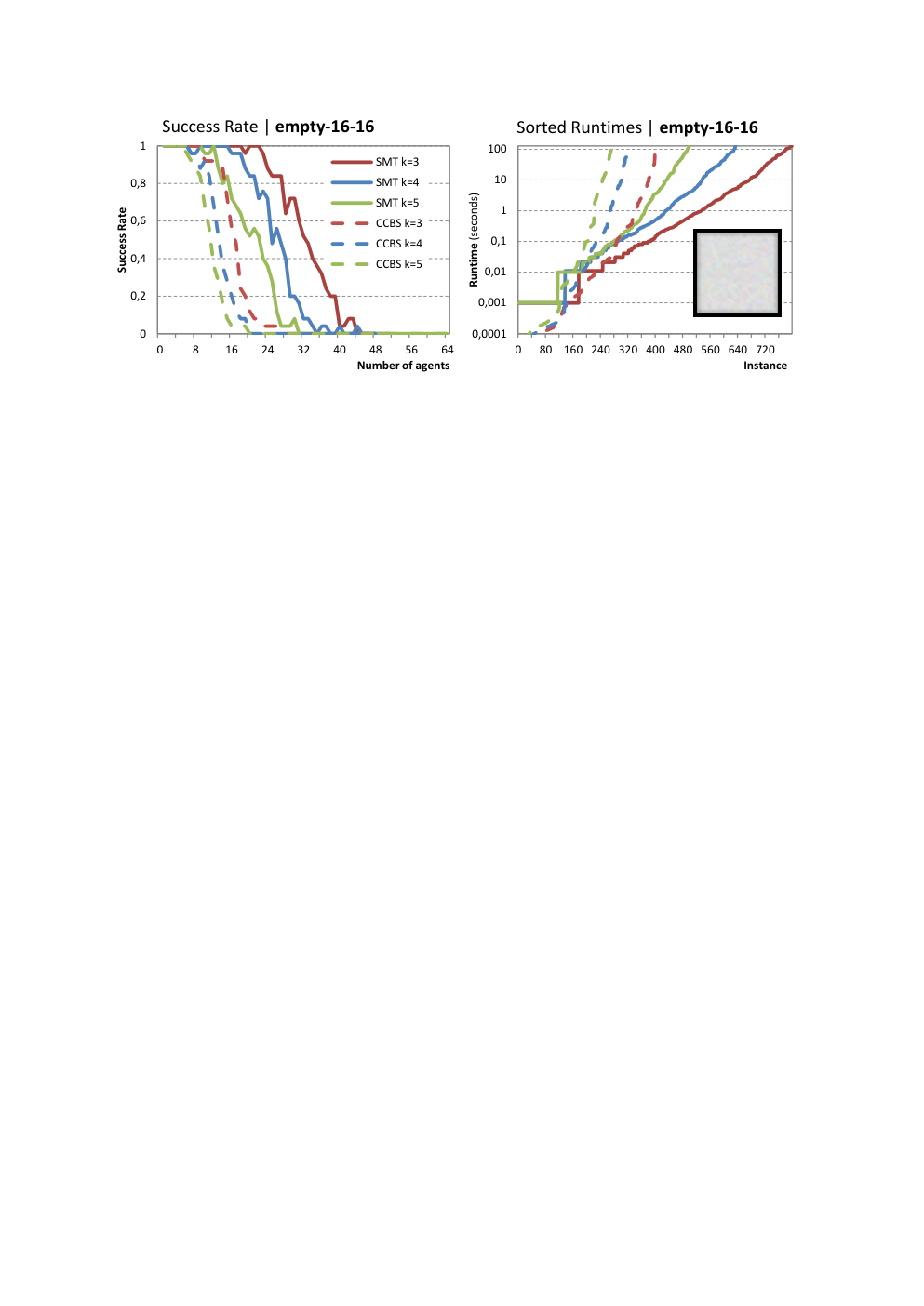
Part of the results obtained in our experimentation is presented in this section. For each presented benchmark we show success rate as a function of the number of agents. That is, we calculate the ratio out of 25 instances per number of agents where the tested algorithm finished under the timeout of 120 seconds. In addition to this, we also show concrete runtimes sorted in the ascending order. Results for one selected representative benchmark from each category are shown in Figures 3, 4, and 5.

Figure 4: Comparison of SMT-CBS^R and CCBS on $\mathtt{maze}$-$\mathtt{32}$-$\mathtt{32}$-$\mathtt{4}$.

The observable trend is that the difficulty of the problem increases with increasing size of the $K-$neighborhood with notable exception of $\mathtt{maze}$-$\mathtt{32}$-$\mathtt{32}$-$\mathtt{4}$ for $K=4$ and $K=5$ which turned out to be easier than $K=3$ for SMT-CBS^R.

Throughout all benchmarks SMT-CBS^R tends to outperform CCBS. The dominance of SMT-CBS^R is most visible in medium sized benchmarks. CCBS is, on the other hand, faster in instances containing few agents. The gap between SMT-CBS^R and CCBS is smallest in large maps where SMT-CBS^R struggles with relatively big overhead caused by the big size of the map (the encoding is proportionally big). Here SMT-CBS^R wins only in hard cases.

4 Discussion and Conclusion

We suggested a novel algorithm for the makespan optimal solving of the multi-agent path finding problem in continuous time and space called SMT-CBS^R based on satisfiability modulo theories (SMT). Our approach builds on the idea of treating constraints lazily as suggested in the CBS algorithm but instead of branching the search after encountering a conflict we refine the propositional model with the conflict elimination disjunctive constraint as it has been done in previous application of SMT in the standard MAPF.

Figure 5: Comparison of SMT-CBS^R and CCBS on $\mathtt{ost003d}$.

The major obstacle in using SMT and propositional reasoning not faced previously with the standard MAPF is that decision variables cannot be determined in advance straightforwardly in the continuous case. We hence suggested a novel decision variable generation approach that enumerates new decisions after discovering new collisions.

We compared SMT-CBS^R with CCBS [1], currently the only alternative algorithm for MAPF^R that modifies the standard CBS algorithm, on a number of benchmarks. The outcome of our comparison is that SMT-CBS^R performs well against CCBS. The best results SMT-CBS^R are observable on medium sized benchmarks with regular obstacles. We attribute the better runtime results of SMT-CBS^R to more efficient handling of disjunctive conflicts in the underlying SAT solver through propagation, clause learning, and other mechanisms. On the other hand SMT-CBS^R is less efficient on large instances with few agents.

For the future work we assume extending the concept of SMT-based approach for MAPF^R with other cumulative cost functions other than the makespan such as the sum-of-costs [26, 8]. We also plan to extend the RDD generation scheme to directional agents where we need to add the third dimension in addition to space (vertices) and time: direction (angle). The work on MAPF^R could be further developed into multi-robot motion planning in continuous configuration spaces [16].

References

- [1] Andreychuk, A., Yakovlev, K.S., Atzmon, D., Stern, R.: Multi-agent pathfinding with continuous time. In: Proceedings of IJCAI 2019. pp. 39–45 (2019)
- [2] Audemard, G., Simon, L.: Predicting learnt clauses quality in modern SAT solvers. In: IJCAI. pp. 399–404 (2009)
- [3] Balyo, T., Heule, M.J.H., Järvisalo, M.: SAT competition 2016: Recent developments. In: AAAI 2017. pp. 5061–5063 (2017)
- [4] Biere, A., Biere, A., Heule, M., van Maaren, H., Walsh, T.: Handbook of Satisfiability. IOS Press (2009)
- [5] Bofill, M., Palahí, M., Suy, J., Villaret, M.: Solving constraint satisfaction problems with SAT modulo theories. Constraints 17(3), 273–303 (2012)
- [6] Botea, A., Surynek, P.: Multi-agent path finding on strongly biconnected digraphs. In: AAAI. pp. 2024–2030 (2015)
- [7] Cáp, M., Novák, P., Vokrínek, J., Pechoucek, M.: Multi-agent RRT: sampling-based cooperative pathfinding. In: Proceedings of AAMAS 2013. pp. 1263–1264 (2013)
- [8] Felner, A., Li, J., Boyarski, E., Ma, H., L.Cohen, Kumar, T.K.S., Koenig, S.: Adding heuristics to conflict-based search for multi-agent path finding. In: Proceedings of ICAPS 2018. pp. 83–87 (2018)
- [9] Hönig, W., Kumar, T.K.S., Cohen, L., Ma, H., Xu, H., Ayanian, N., Koenig, S.: Summary: Multi-agent path finding with kinematic constraints. In: Proceedings of IJCAI 2017. pp. 4869–4873 (2017)
- [10] Janovsky, P., Cáp, M., Vokrínek, J.: Finding coordinated paths for multiple holonomic agents in 2-d polygonal environment. In: Proceedings of AAMAS 2014. pp. 1117–1124 (2014)
- [11] Kautz, H.A.: Deconstructing planning as satisfiability. In: Proceedings, The Twenty-First National Conference on Artificial Intelligence and the Eighteenth Innovative Applications of Artificial Intelligence Conference, 2006. pp. 1524–1526. AAAI Press (2006)
- [12] Kautz, H.A., Selman, B.: Planning as satisfiability. In: Proceedings ECAI 1992. pp. 359–363 (1992)
- [13] Kautz, H.A., Selman, B.: Pushing the envelope: Planning, propositional logic and stochastic search. In: Proceedings of AAAI 1996. pp. 1194–1201 (1996)
- [14] Kautz, H.A., Selman, B.: Unifying sat-based and graph-based planning. In: Proceedings of IJCAI 1999. pp. 318–325 (1999)
- [15] Kornhauser, D., Miller, G.L., Spirakis, P.G.: Coordinating pebble motion on graphs, the diameter of permutation groups, and applications. In: FOCS, 1984. pp. 241–250 (1984)
- [16] LaValle, S.M.: Planning algorithms. Cambridge University Press (2006)
- [17] Li, J., Surynek, P., Felner, A., Ma, H., Koenig, S.: Multi-agent path finding for large agents. In: Proceedings of AAAI 2019. AAAI Press (2019)
- [18] Ma, H., Koenig, S., Ayanian, N., Cohen, L., Hönig, W., Kumar, T.K.S., Uras, T., Xu, H., Tovey, C.A., Sharon, G.: Overview: Generalizations of multi-agent path finding to real-world scenarios. CoRR abs/1702.05515 (2017), http://arxiv.org/abs/1702.05515
- [19] Ma, H., Wagner, G., Felner, A., Li, J., Kumar, T.K.S., Koenig, S.: Multi-agent path finding with deadlines. In: Proceedings of IJCAI 2018. pp. 417–423 (2018)
- [20] Nieuwenhuis, R.: SAT modulo theories: Getting the best of SAT and global constraint filtering. In: Proceedings of CP 2010. pp. 1–2 (2010)
- [21] Phillips, M., Likhachev, M.: SIPP: safe interval path planning for dynamic environments. In: Proceedings of ICRA 2011. pp. 5628–5635 (2011)
- [22] Ratner, D., Warmuth, M.K.: Nxn puzzle and related relocation problem. J. Symb. Comput. 10(2), 111–138 (1990)
- [23] Rivera, N., Hernández, C., Baier, J.A.: Grid pathfinding on the 2k neighborhoods. In: Proceedings of AAAI 2017. pp. 891–897 (2017)
- [24] Ryan, M.R.K.: Exploiting subgraph structure in multi-robot path planning. J. Artif. Intell. Res. (JAIR) 31, 497–542 (2008)
- [25] Sharon, G., Stern, R., Felner, A., Sturtevant, N.: Conflict-based search for optimal multi-agent pathfinding. Artif. Intell. 219, 40–66 (2015)
- [26] Sharon, G., Stern, R., Goldenberg, M., Felner, A.: The increasing cost tree search for optimal multi-agent pathfinding. Artif. Intell. 195, 470–495 (2013)
- [27] Silver, D.: Cooperative pathfinding. In: AIIDE. pp. 117–122 (2005)
- [28] Stern, R.: Multi-agent path finding - an overview. In: Osipov, G.S., Panov, A.I., Yakovlev, K.S. (eds.) Artificial Intelligence - 5th RAAI Summer School. Lecture Notes in Computer Science, vol. 11866, pp. 96–115. Springer (2019)
- [29] Sturtevant, N.R.: Benchmarks for grid-based pathfinding. Computational Intelligence and AI in Games 4(2), 144–148 (2012)
- [30] Surynek, P.: A novel approach to path planning for multiple robots in bi-connected graphs. In: ICRA 2009. pp. 3613–3619 (2009)
- [31] Surynek, P.: Conflict handling framework in generalized multi-agent path finding: Advantages and shortcomings of satisfiability modulo approach. In: Rocha, A.P., Steels, L., van den Herik, H.J. (eds.) Proceedings of the 11th International Conference on Agents and Artificial Intelligence, ICAART 2019, Volume 2. pp. 192–203. SciTePress (2019)
- [32] Surynek, P.: Lazy compilation of variants of multi-robot path planning with satisfiability modulo theory (SMT) approach. In: 2019 IEEE/RSJ International Conference on Intelligent Robots and Systems, IROS 2019. pp. 3282–3287. IEEE (2019)
- [33] Surynek, P.: Multi-agent path finding with continuous time and geometric agents viewed through satisfiability modulo theories (SMT). In: Surynek, P., Yeoh, W. (eds.) Proceedings of the Twelfth International Symposium on Combinatorial Search, SOCS 2019. pp. 200–201. AAAI Press (2019)
- [34] Surynek, P.: Multi-agent path finding with continuous time viewed through satisfiability modulo theories (SMT). CoRR abs/1903.09820 (2019), http://arxiv.org/abs/1903.09820
- [35] Surynek, P.: Unifying search-based and compilation-based approaches to multi-agent path finding through satisfiability modulo theories. In: Proceedings of IJCAI 2019. pp. 1177–1183 (2019)
- [36] Surynek, P.: On satisfisfiability modulo theories in continuous multi-agent path finding: Compilation-based and search-based approaches compared. In: Rocha, A.P., Steels, L., van den Herik, H.J. (eds.) Proceedings of the 12th International Conference on Agents and Artificial Intelligence, ICAART 2020, Volume 2, 2020. pp. 182–193. SCITEPRESS (2020)
- [37] Surynek, P., Felner, A., Stern, R., Boyarski, E.: Efficient SAT approach to multi-agent path finding under the sum of costs objective. In: ECAI. pp. 810–818 (2016)
- [38] Tinelli, C.: Foundations of satisfiability modulo theories. In: Proceedings is WoLLIC 2010. p. 58 (2010)
- [39] Walker, T.T., Sturtevant, N.R., Felner, A.: Extended increasing cost tree search for non-unit cost domains. In: Proceedings of IJCAI 2018. pp. 534–540 (2018)
- [40] Wang, K., Botea, A.: MAPP: a scalable multi-agent path planning algorithm with tractability and completeness guarantees. JAIR 42, 55–90 (2011)
- [41] Yu, J., LaValle, S.M.: Optimal multi-robot path planning on graphs: Structure and computational complexity. CoRR abs/1507.03289 (2015)