Address for correspondence: Vinícius Mayrink, Departamento de Estatística, ICEx, UFMG. Av. Antônio Carlos, 6627, Belo Horizonte, MG, Brazil, 31270-901. E-mail: vdm@est.ufmg.br

Abstract

In this study, we present a new module built for users interested in a programming language similar to BUGS to fit a Bayesian model based on the piecewise exponential (PE) distribution. The module is an extension to the open-source program JAGS by which a Gibbs sampler can be applied without requiring the derivation of complete conditionals and the subsequent implementation of strategies to draw samples from unknown distributions. The PE distribution is widely used in the fields of survival analysis and reliability. Currently, it can only be implemented in JAGS through methods to indirectly specify the likelihood based on the Poisson or Bernoulli probabilities. Our module provides a more straightforward implementation and is thus more attractive to the researchers aiming to spend more time exploring the results from the Bayesian inference rather than implementing the Markov Chain Monte Carlo (MCMC) algorithm. For those interested in extending JAGS, this work can be seen as a tutorial including important information not well investigated or organized in other materials. Here, we describe how to use the module taking advantage of the interface between R and JAGS. A short simulation study is developed to ensure that the module behaves well and a real illustration, involving two PE models, exhibits a context where the module can be used in practice.

keywords: MCMC, Bayesian Inference, Semiparametric, Survival Analysis.

1 Introduction

The piecewise exponential (PE) modeling is a simple approach extensively used in survival analysis and reliability to approximate the distribution of event-time data; possibly investigating the association of the time response with explanatory variables. Applications related to clinical data can be easily found in the literature; for example: leukemia (Breslow, 1974), gastric cancer (Gamerman, 1991), kidney infection (Sahu et al., 1997; Ibrahim et al., 2001), breast cancer (Sinha et al., 1999), melanoma (Demarqui et al., 2014) and hospital mortality (Clark and Ryan, 2002). In the context of reliability, consider the maintenance analysis in Rigdon and Basu (2000) and the telecommunication study in Kim and Proschan (1991) and Gamerman (1994), among many other references.

The PE models are classified as semiparametric due to their flexibility to represent the hazard function without making strong and restrictive parametric assumptions regarding the shape of this component; this point makes the PE distribution very attractive for survival analysis. Its semiparametric nature allows considerable generality and enough structure for useful interpretations in any application. The popularity of semiparametric methods for univariate survival data started with Cox (1972) on the proportional hazards model. Breslow (1972) and Breslow (1974) proposed the use of the PE distribution to replace the baseline term and Kalbfleisch and Prentice (1973) investigated the grid configuration. In this paper, we are focused on PE models under the Bayesian approach for inference, which has been widely considered in the literature. See Ibrahim et al. (2001) for a broad presentation of Bayesian survival models and Sinha and Dey (1997) for a review on Bayesian semiparametric frameworks (including the PE) based on either the hazard or the intensity function.

Implementing a PE model is an obstacle for those interested in a Bayesian analysis and having limited programming skills. In many cases, the main source of this difficulty is the use of an indirect method to draw samples from the unknown joint posterior distribution. The Markov Chain Monte Carlo (MCMC) algorithm Gibbs sampling (Geman and Geman, 1984; Gelfand and Smith, 1990; Gamerman and Lopes, 2006, see) is widely applied for this task, and its implementation can be very demanding due to the sequential simulations from complete conditional posterior distributions. This is particularly true when the conjugate analysis is not possible leading to a Gibbs sampler whose steps depend on other methods – e.g., Metropolis-Hastings (Metropolis et al., 1953; Hastings, 1970), Adaptive Rejection Sampling (Gilks and Wild, 1992; Gilks, ), Adaptive Rejection Metropolis Sampling (Gilks et al., 1995) and Slice Sampling (Neal, 2003).

As an alternative to simplify the Gibbs sampler implementation for a given model, one can take advantage of programs based on a dialect of the BUGS language (Thomas et al., 1992; Lunn et al., 2012) using the mathematical formalism of directed acyclic graphs to define joint densities. These programs build the whole structure of complete conditionals and their corresponding sampling strategies requiring from the user only the essential information related to the model fit (priors, likelihood and the MCMC setup). In this category, WinBUGS (Spiegelhalter et al., 2003), OpenBUGS (Spiegelhalter et al., 2014) and JAGS (Plummer, 2003) are three well known options. In particular, JAGS is an appealing case since it is open-source (released under a free copyleft license) and extensible allowing users with C++ knowledge to create functions, monitors, distributions and samplers for a new module. These features enable the potential formation of a future JAGS contributor community similar to that of the software R (Team, 2020).

Other alternatives are available as a support for the Bayesian computing. A well known case is the platform Stan (mc-stan.org), having an interface with R through the package rstan (Stan Development Team, 2019). The MCMC method applied here is called No-U-Turn Sampling (Hoffman and Gelman, 2014), being an extension of the Hamiltonian Monte Carlo method. Implementing new distributions in Stan is straightforward and it does not require the installation of new modules. However, due to the Hamiltonian dynamics to improve sampling, one cannot set discrete prior distributions. This is perhaps the greatest weakness of Stan. Another possibility to deal with Bayesian modeling in R is the package BayesX (Brezger et al., 2005). However, this alternative was designed for the framework of generalized linear models, where the distribution of the response variable belongs to the exponential family. This is not the case for survival models assuming the PE distribution. Bayesian computing can also be developed via INLA (Rue et al., 2009); further details in r-inla.org. This option performs approximate Bayesian inference on the class of latent Gaussian models. It handles non-Gaussian likelihoods, but the presence of non-Gaussian latent components can be a limitation; for example, assuming a discrete or a multimodal distribution for a random effect would be problematic.

The main contribution of this work is to present a new JAGS module (pexm) for Bayesian analyses involving the PE distribution. An R package, having the same name, was developed to install and load the tool. The proposed module was created to fill a gap existing in JAGS related to the absence of the PE distribution. The pexm allows a friendlier and cleaner model implementation, being attractive for many users. Computational speed is also an advantage of the proposal with respect to the usual implementation based on the Poisson zeros-trick. Another important contribution is a description to clarify some aspects related to the topic “extending JAGS”, which is not well documented in the literature. There are no formal tutorials exploring the technical elements detailed in Appendix A. The JAGS manuals (Plummer, 2010; Plummer, 2017) do not currently contain the mentioned information, however, these materials can be updated in the future.

The outline of this paper is as follows: in Section 2, we describe the elements of the PE distribution implemented in the proposed JAGS module. In Section 3, we present an overview on how the module was created, explain how to use it from within R, discuss the main simplifications with respect to an implementation without the module and develop a simulation study to verify the performance. Section 4 shows results (with and without the module) in a real application involving two frailty models to fit a kidney infection data (Ibrahim et al., 2001); the rates and log-rates in adjacent intervals are correlated via gamma and normal priors, respectively. Finally, Section 5 presents the conclusions and final remarks.

2 The piecewise exponential distribution

The PE distribution requires the specification of a grid $\tau=\{a_{1},a_{2},\ldots,a_{m}\}$ partitioning the time axis into $m$ intervals. Let $a_{1}=0$, $a_{m}<+\infty$ and $a_{m+1}=+\infty$; the latter is defined only for notation purposes and it is not expressed in $\tau$. Conditional on this time grid, the failure rate $\lambda_{j}$ is assumed constant inside the corresponding interval: $I_{j}=(a_{j},a_{j+1}]$ for $j=1,\ldots,m-1$ and $I_{m}=(a_{m},+\infty)$ for $j=m$. This step function formulation provides a discrete version of the true unknown hazard function in a survival model. Assume that $T$ is a continuous non-negative random variable representing the survival times of subjects in a population. Let $f(t)$ denote the probability density function (pdf) of $T$, $F(t)$ is the associated cumulative distribution function (cdf), $S(t)=1-F(t)$ is the survival function, $h(t)$ is the hazard function and, finally, $H(t)$ represents the cumulative hazard function. If $T\sim\mbox{PE}(\lambda,\tau)$ with $\lambda=\{\lambda_{1},\ldots,\lambda_{m}\}$, then:

$$h(t)=\lambda_{j},\;\;\mbox{if}\;\;t\in I_{j},\;\;j=1,\ldots,m.$$ (1)

Naturally, the quality of the approximation to the real hazard function depends on a suitable choice of the time grid $\tau$. In Breslow (1972) the author suggests the use of the observed failure times as the limits of the intervals $I_{j}$; however, depending on the sample size, this can lead to a non-parsimonious model with many rates $\lambda_{j}$ to be estimated. In contrast, Kalbfleisch and Prentice (1973) indicates that the grid should be selected independently of the data. The study explores different interval sizes configuring a regular grid. When choosing $\tau$ without using the data, one might consider two aspects: small $m$ leads to a poor discretization and a large $m$ determines a non-parsimonious model. Irregular grids are also allowed in the analysis and this could be a reasonable strategy in applications assuming higher frequency of failures in certain parts of the time axis; i.e., wider intervals would be specified for time regions where few events are expected to be observed.

The cumulative hazard function is expressed as follows:

$$H(t)=\left\{\begin{array}[]{l}\lambda_{1}\,t,\;\;\mbox{if}\;\;t\in I_{1};\\ \lambda_{j}(t-a_{j})+\sum_{i=1}^{j-1}\lambda_{i}(a_{i+1}-a_{i}),\;\;\mbox{if}\;\;t\in I_{j},\;j=2,\ldots,m.\end{array}\right.$$ (2)

We can use (2) to evaluate the survival function at a time point $t$ through the well known equality $S(t)=\exp\{-H(t)\}$. The pdf of $T$ can be easily identified by simply taking the derivative of $F(t)=1-S(t)$ with respect to $t$. This provides $f(t)=h(t)\exp\{-H(t)\}$, where $h(t)$ is given in (1).

The quantile is an information of interest in many data analyses. In the context of the PE distribution, this quantity can be calculated via the relationship $H(t)=-\ln(1-F(t))$. Given a probability $p$, the corresponding quantile is the value $t^{*}$ such that $H(t^{*})=-\ln(1-p)$. Let $w(p)=-\ln(1-p)$ and recall that $H(a_{m+1})=+\infty$. Then, the calculation of $t^{*}$ can be expressed by:

$$t^{*}=\left\{\begin{array}[]{l}a_{1}+\dfrac{w(p)}{\lambda_{1}},\;\;\mbox{if}\;\;w(p)\leq H(a_{2})=\lambda_{1};\\ a_{j}+\dfrac{w(p)-\sum_{i=1}^{j-1}\lambda_{i}(a_{i+1}-a_{i})}{\lambda_{j}},\;\;\mbox{if}\;\;H(a_{j})<w(p)\leq H(a_{j+1}),\,j=2,\ldots,m.\end{array}\right.$$ (3)

Note that we can easily compute the median of the PE distribution by setting $p=0.5$ in (3). Those readers interested in details about the first two moments of the PE distribution can refer to Barbosa et al. (1996).

3 The JAGS module.

JAGS (Plummer, 2003, “Just Another Gibbs Sampler”; see) is a general-purpose, open-source, cross-platform graphical modeling program using a set of MCMC methods for stochastic simulations to generate samples from the joint posterior distribution of the parameters in a Bayesian model. These samples are further used for inferences regarding the target parameters and the model fit. A recent version of JAGS can be downloaded from http://mcmc-jags.sourceforge.net and it is also available as a package for different Linux distributions.

A special feature of JAGS is that it can be modular and extensible with new functionalities, which can be loaded whenever required. A module can be created to accommodate all types of probability distributions (continuous or discrete, univariate or multivariate). In order to write these extensions, the knowledge of C++ and object oriented programming is necessary; however, we emphasize that installing the extensions can be extremely automatic depending on the operational system.

Technical manuals providing a comprehensive coverage on how to build a JAGS module were not available in the literature at the time of writing this material. We follow the steps indicated in Wabersich and Vandekerckhove (2014), which can be seen as a short tutorial exploring the key aspects to add custom distributions to JAGS. Those aspects not covered in this reference, but important to implement the PE distribution, are given careful attention in Appendix A. For instance, the authors in Wabersich and Vandekerckhove (2014) work with two examples: the Bernoulli distribution for didactic purposes and the Wiener diffusion first-passage time distribution. In both cases the input values are scalar quantities; i.e., the paper does not explore distributions with vectors as arguments, which is the case for the $\mbox{PE}(\lambda,\tau)$. This issue can be easily addressed by simply modifying the parent class type expressed in the code from scalar to vector (see Appendix A).

The PE distribution implementation described in Appendix A is in fact a more complete example displaying the use of important resources available to create a JAGS module. Besides implementing the log-density and the sample generating process allowing the MCMC simulations in a Gibbs sampler, we have built auxiliary functions returning the pdf, cdf, quantile, hazard and cumulative hazard of the $\mbox{PE}(\lambda,\tau)$ at a given time $t$ or probability $p$. In addition, the module includes a routine to check whether the values in $\lambda$ and $\tau$ are consistent with the specifications shown in Section 2. Hence, Appendix A contains essential complementary information (Wabersich and Vandekerckhove, 2014, with respect to) to those readers interested in extending JAGS.

3.1 Using the module in the R environment.

In this section, we discuss how to use the proposed module in association with R. This is achieved through the package rjags (Plummer, 2016) providing an interface between R and JAGS. Installing the new module is straightforward as indicated in Appendix A. The procedure basically involves the installation of an R package called pexm. The package was designed for this task and also contains tools to help loading the module into the R environment. The pexm source can be downloaded from two repositories: GitHub and Sourceforge (see more details in Appendix A.3). Hereafter, we assume that a recent version of JAGS, R, rjags and the proposed pexm module are correctly installed in the computer. A confirmation that the module is ready to be used in R can be obtained by simply typing the following commands in the console:

⬇

1 R> library("pexm")

2 R> loadpexm()

In order to illustrate how to use the module, we have developed a simple example taking into account the R package msm (Jackson, 2011) to generate the data. This package provides functions to fit continuous-time Markov and hidden Markov multi-state models and, in particular, includes the function rpexp to draw samples from the PE distribution. We can also use dpexp, ppexp and qpexp to explore the pdf, cdf and quantiles.

Let $T_{i}$ be the survival time of the $i$-th individual, $i=1,\ldots,n$. In our illustration, we set the real rates $\lambda=(0.3,0.6,0.8,1.3)^{\top}$, the time grid $\tau=\{0,2,3,5\}$, $n=1{,}000$ and assume $T_{i}\sim\mbox{PE}(\lambda,\tau)$ to generate the data. The following objects are loaded into the R workspace: t is the observed vector $(T_{1},\ldots,T_{n})^{\top}$, n is the length of t, tau is the grid vector, m is the length of tau, pq is a vector of probabilities for which the quantile should be evaluated, and nq is the length of pq.

Code chunk CC.1:

⬇

1 R> data <- list(t = t, n = n, tau = tau, m = m, pq = pq, nq = nq)

2 R> parameters <- c("lambda", "ht100", "Ht100", paste0("q[",1:nq,"]"), paste0("loglik[",1:n,"]"), paste0("St[",1:n,"]"))

3 R> inits1 <- list( lambda = c(0.1, 0.5, 1, 2), .RNG.name = "base::Super-Duper", .RNG.seed = 1 )

4 R> inits2 <- list( lambda = c(0.5, 1.0, 1.5, 2.5), .RNG.name = "base::Wichmann-Hill", .RNG.seed = 2 )

5 R> burnin <- 1000

6 R> lag <- 1

7 R> npost <- 2000

8 R> Mjags <- rjags::jags.model(file = "Model_pex.R", data = data, inits = list(inits1, inits2), n.chains = 2, n.adapt = burnin)

9 R> output <- rjags::coda.samples(Mjags, variable.names = parameters, n.iter = npost, thin = lag)

The Code chunk CC.1 shows a simple R script to organize the workspace information and then access JAGS for the MCMC simulation. Note that we specify: a list object (data) containing t, n, tau, m, pq and nq; a string vector (parameter) indicating which chains must be saved; two list objects (inits1 and inits2) providing initial values for $\lambda$ and setting details about random seeds in JAGS. The MCMC setup is determined through the elements: size of the burn-in period (burnin), thinning interval of the chains (lag) and the number of posterior samples required for inference (npost). The last two commands, jags.model and coda.samples, are functions from the library rjags to compile the Bayesian model in Model_pex.R (written in the JAGS syntax) and to run the corresponding MCMC algorithm, respectively. It is important to emphasize that the Code chunk CC.1 assumes that the R working directory is the same one where the model script Model_pex.R is located. Note that we choose to handle the results in a format that can be conveniently analyzed via the R package coda (Plummer et al., 2006). Results are saved in the object output. The posterior estimates discussed ahead are based on the two chains generated for each parameter.

Code chunk CC.2

⬇

1 model{

2 for (i in 1:n) {

3 t[i] ~ dpex(lambda[], tau[])

4 St[i] <- 1 - ppex(t[i], lambda[], tau[])

5 loglik[i] <- log(dpex(t[i], lambda[], tau[]))

6 }

7 Ht100 <- hcpex(t[100], lambda[], tau[])

8 ht100 <- hpex(t[100], lambda[], tau[])

9 for (j in 1:m) { lambda[j] ~ dgamma(0.01, 0.01) }

10 for (k in 1:nq) { q[k] <- qpex(pq[k], lambda[], tau[]) }

11 }

The content of the JAGS model script Model_pex.R is presented in the Code chunk CC.2. This code indicates the likelihood $T_{i}\sim\mbox{PE}(\lambda,\tau)$ and the prior specifications $\lambda_{j}\sim\mbox{Ga}(0.01,0.01)$ for $j=1,\ldots,m$ (mean $1$ and variance $100$). Note that in each iteration of the MCMC, the survival function St[i] and the log-density loglik[i] are evaluated for each $t_{i}$ together with the quantile q[k] for the probabilities in pq. In addition, the cummulative hazard function Ht100 and the hazard function ht100, related to the time point $t_{100}$, are monitored in this example. As it can be seen, the elements defined in Model_pex.R explore all functionalities implemented for the PE distribution in the new module.

3.2 Strategies to indirectly specify the likelihood.

Without the proposed pexm module, one can use either the Poisson or the Bernoulli distribution to indirectly specify the likelihood function. These strategies are commonly known as zeros-trick (Lunn et al., 2012) and ones-trick (Spiegelhalter et al., 2003), respectively. Let $l_{i}=\ln[f(t_{i}|\lambda,\tau)]$, then the likelihood can be written as:

$$f(t_{1},\ldots,t_{n}|\theta)\;=\;\prod_{i=1}^{n}\exp\{l_{i}\}\;=\;\prod_{i=1}^{n}\dfrac{\exp\{-(-l_{i})\}(-l_{i})^{0}}{0!}\;=\;\prod_{i=1}^{n}P(X_{i}=0),$$

where $X_{i}\sim\mbox{Pois}(-l_{i})$. In order to ensure a positive Poisson mean, we can select a constant $C>0$ and use:

$$\exp\{-C\}\;f(t_{1},\ldots,t_{n}|\theta)\;=\;\prod_{i=1}^{n}\dfrac{\exp\{-(-l_{i}+C)\}(-l_{i}+C)^{0}}{0!}\;=\;\prod_{i=1}^{n}P(X_{i}^{*}=0),$$

where $X_{i}^{*}\sim\mbox{Pois}(-l_{i}+C)$. We must choose $C$ such that $-l_{i}+C>0$ for all $i=1,\ldots,n$. Note that adding $C$ does not affect the inference results, since it is equivalent to multiplying the posterior distribution by a constant term.

Code chunk CC.3

⬇

1 model {

2 C <- 10000

3 for (i in 1:n) {

4 zeros[i] ~ dpois( zero_mean[i] )

5 zero_mean[i] <- -l[i] + C

6 l[i] <- ... # log-likelihood here.

7 }

8 ... # Priors and other terms here.

9 }

This strategy can be applied in JAGS using the syntax shown in Code chunk CC.3. Note that the log-likelihood of the $\mbox{PE}(\lambda,\tau)$ for the $i$-th observation must be specified for the object l[i]. This task for the PE context is not simple compared to other distributions. A possible approach is to replace the vector t and tau by other objects accounting for the position of each observed time point in the grid. These objects must be created in the R environment and passed to JAGS as a data argument (see data in the Code chunk CC.1) together with zero[i] = 0 for all $i$. They must allow the calculation of $H(t)$ in JAGS, which in turn can be used to obtain $\ln[f(t)]=\lambda_{j}-H(t)$ (if $t\in I_{j}$) and $S(t)=\exp\{-H(t)\}$. After the MCMC simulation, the quantiles can be calculated in R using the posterior samples of $\lambda$ and the function qpexp (package msm).

Again, we call attention to the fact that the Bernoulli distribution can also be used in a similar strategy expressing the model likelihood as $\prod_{i=1}^{n}P(X_{i}^{*}=1)$ with $X_{i}^{*}\sim\mbox{Bern}(\exp\{l_{i}-C\})$. Although both approaches have the same goal, the Poisson-zeros option is more popular in the literature.

The main conclusion of this section is that the pexm module provides a simpler and more attractive implementation of a Bayesian PE model in JAGS, since it avoids the use of alternative strategies to indirectly specify the likelihood. In the next section, we develop two types of studies using artificial data sets. The first one compares the results from the model in Code chunk CC.2 and those obtained via the msm package. The second study is intended to evaluate the performance of pexm with respect to the Poisson-zeros strategy. In Section 4, the analysis “pexm versus zeros-trick” is based on a real data set and it accounts for scripts (zeros-trick case) suggested in Ibrahim et al. (2001).

3.3 Simulation study.

The first goal of the present section is to verify whether the proposed JAGS module is correctly implemented and working as expected. In order to carry out this type of analysis, we consider the configuration described in Section 3.1 to generate a sample of $1{,}000$ time points from the PE distribution; the function rpexp (package msm) is applied here. In each interval defined by $\tau$, we have observed the following number of time points: 443 in $I_{1}$, 247 in $I_{2}$, 245 in $I_{3}$ and 65 in $I_{4}$.

The R script shown in Code chunk CC.1 is used to run the MCMC for the simple PE model indicated in Code chunk CC.2. The argument data is set to evaluate nq = 23 different quantiles corresponding to probabilities in pq ranging from $0.01$ to $0.99$. A good behavior is confirmed, if all posterior estimates for $\lambda$ are close to their corresponding real values (see Section 3.1) and the chain built for each log-density, survival function and quantile is centered around the true value calculated through one of the existing PE functions of the package msm. Figure 1 (a) clearly indicates this mentioned configuration. The three graphs show all true values (grey points) inside the $95\%$ HPD (Highest Probability Density) intervals obtained based on the results from JAGS. In this paper, all HPD intervals are calculated through the R package coda. Other interesting aspects can be observed in Panel (a): ($i$) the shape and decay speed of the survival function; ($ii$) the log density formed by four different parts corresponding to each interval $I_{j}$; ($iii$) the higher posterior uncertainty expressed in the log-density related to $I_{4}$. The behavior indicated in ($iii$) is justified by the fact that only 65 time-points belong to the last grid interval, meaning less information to estimate $\lambda_{4}$.

Figure 1 (b) shows the chains generated for each $\lambda_{j}$ after the burn-in period. As it can be seen, the convergence to the real values (horizontal lines) is visually confirmed and low autocorrelation is observed for all cases (recall that lag = 1). Here, all real values can be found within the corresponding $95\%$ HPD intervals, and the posterior mean and median approximate well their targets. In terms of variability, the standard deviations can be ordered as follows: $0.013\,(\lambda_{1})<0.037\,(\lambda_{2})<0.050\,(\lambda_{3})<0.165\,(\lambda_{4})$. Again, a larger number of observations in $I_{j}$ leads to a smaller posterior variability for $\lambda_{j}$.

The Code chunk CC.2 contains the pexm functions hpex and hcpex, which are alternatives to calculate during the MCMC run the hazard function (1) and the cumulative hazard function (2), respectively. Note that this JAGS model script is set to evaluate these functions for $t_{100}=3.483$. Since $\tau=\{0,2,3,5\}$, we have $t_{100}\in I_{3}$ and thus $h(t_{100})=\lambda_{3}$. The posterior sample related to the object ht100 provides the mean $0.778$ (the true $\lambda_{3}$ is $0.8$). The posterior mean of the cumulative hazard Ht100 is $1.529$ (the true value is $1.587$). This average can also be obtained using the relationship $H(t)=-\ln[S(t)]$. A final remark related to these functions is that the present example can be extended to the survival regression setting. One might be interested in evaluating $h(t)$ or $H(t)$ under the effect of some fixed configuration of covariates. This can be easily adapted to hpex and hcpex by including the covariates effects in the argument lambda; Section 4 discusses two models having a regression setting.

(a)

(b)

Figure 1: Comparison of posterior estimates (mean and $95\%$ HPD interval) obtained from JAGS (black) and the values calculated via msm package (grey points). Panel (a): log-density and survival function for each observation $t_{i}$ and quantiles for different probabilities. Panel (b): trace plots representing the two chains (in red and black after the burn-in period) for each $\lambda_{j}$; horizontal lines (blue) indicate the real values.

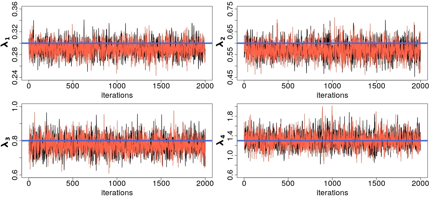
Monte Carlo scheme.

The second investigation developed in this section is based on a Monte Carlo (MC) scheme with 100 replications, i.e., we evaluate 100 data sets generated under the same conditions. The main aim here is to compare the performances of a Bayesian model implemented with the module pexm and another version using the Poisson-zeros strategy (zeros-trick). We emphasize that the difference here is only the JAGS syntax. The model to be fitted is a simplification of the one exhibited in the Code chunk CC.2. We will not save results related to the quantiles, survival, hazard and cumulative hazard functions. In the pexm case, we only specify the likelihood via t[i]   dpex(lambda[], tau[]) and the prior lambda[j]   dgamma(0.01, 0.01). On the other hand, the Poisson-zeros case is defined as indicated in Code chunk CC.3, where the log-likelihood related to the PE distribution must be written for the object l[i]; we also set $\lambda_{j}\sim\mbox{Ga}(0.01,0.01)$. Using this simple model, we evaluate “pexm versus zeros-trick” based on the MCMC outputs associated to the rates $\lambda_{j}$’s.

In order to generate the data sets, consider the steps: ($i$) set the grid $\tau=\{0,2,3,5\}$ establishing 4 intervals, ($ii$) choose the sample size $n$, ($iii$) define the true $\lambda$ and ($iv$) generate time observations from the PE distribution using the function rpexp from the R package msm. In the present analysis, we explore three scenarios of configurations for the true $\lambda$: increasing $\lambda=\{0.3,0.6,0.8,1.3\}$ (Scenario 1 or S1), constant $\lambda=\{0.7,0.7,0.7,0.7\}$ (Scenario 2 or S2) and decreasing $\lambda=\{1.3,0.8,0.6,0.3\}$ (Scenario 3 or S3). In addition to these scenarios, we evaluate two sample sizes ($n=100$ and $n=1{,}000$ time points).

For both implementations, the MCMC is configured with burn-in $=1{,}000$, lag $=1$ and $2{,}000$ posterior samples collected after the warm-up period. Two chains are obtained for each parameter. These chains are combined to calculate all descriptive statistics; except the effective sample size (using only the first chain). The starting values in the algorithm are also the same for both strategies; we highlight that the arguments .RNG.name and .RNG.seed, see the rjags documentation, were fixed to impose the same settings of random number generators in JAGS. The algorithms for all combinations of scenarios and sample sizes were executed in the same computer (Intel Core i7 processor and 16.00 GB memory) dedicated exclusively for this task.

$$\begin{array}[]{ccc}(\mbox{a})&&(\mbox{b})\\ \includegraphics[width=169.11208pt]{comptime_MCsim.jpeg}&&\includegraphics[width=206.69333pt]{effsize_MCsim.jpeg}\\ \end{array}$$

Figure 2: Boxplots summarizing the results from the MC scheme. Graphs in light blue (left) are related to the implementation via pexm. Graphs in light red (right) correspond to the Poisson-zeros strategy. Panel (a) shows the computational times required by JAGS to run the MCMC (Column 1 indicates $n=100$, Column 2 indicates $n=1{,}000$). Panel (b) presents the effective sample sizes of the chains generated for each $\lambda_{j}$ (Column 1 indicates $n=100$, Column 2 indicates $n=1{,}000$). In both panels, the scenarios S1, S2 and S3 are represented in the rows 1, 2 and 3, respectively.

Figure 2 shows boxplots summarizing some of the most interesting results from the MC scheme. Thys type of graph is a good option in studies involving replications, since it indicates the variability of repeated measurements (Monte Carlo error) through the length of the boxes. Panel (a) presents the computational times (in seconds) needed to run the Gibbs sampling via JAGS. Theses values were determined through the existing function proc.time in R. The graphs in Panel (b) indicate the effective sample size of the chains obtained for the $\lambda_{j}$’s. This quantity was calculated using the function effectiveSize available in the R package coda. The light blue color represents the implementation based on the module pexm; light red is related to the Poisson-zeros strategy. Given that the same data set is being fitted by the same model with different implementations, this is done in a controlled setting for reproducibility, we have observed the exact same results from the corresponding MCMC runs. In other words, the outcomes of pexm and zeros-trick are the same in the comparison of bias, coverage percentages and autocorrelation. This aspect is clearly noted in Panel (b).

In many studies, the computational time is measured in terms of the processor time used by each implementation to achieve a given effective sample size. This alternative cannot be applied here due to the mentioned compatibility of results. Instead, we focus on the required time to run $3{,}000$ MCMC iterations for each artificial data set. Figure 2 (a) presents the main difference between pexm and the zeros-trick. Naturally, the computational times related to $n=100$ are smaller than those for fitting $n=1{,}000$; please, note the distinct scales in the y-axis to allow visualization. For all combinations (scenario, $n$), the boxplots associated with pexm are located in a lower level than those for the zeros-trick. This suggests that the computational speed is an advantage of the module.

Figure 2 also indicates that the differences between the scenarios S1, S2 and S3 are more evident for the case $n=100$. Note that the variability exhibited by the graphs are higher in (S3, $n=100$). Few distinctions are detected between the scenarios when $n=1{,}000$. Panel (b) suggests that the effective sample size related to $\lambda_{1}$ tend to be higher than those for the other rates. Recall, from the previous study, that the true $\lambda$ in S1 provides few time points generated in the last interval of the grid ($t_{i}>5$). This feature also occurs for the choices of $\lambda$ in S2 and S3. When comparing the number of cases $t_{i}>5$, we have the following order S1 ¿ S2 ¿ S3. The small number of observations in the last interval (especially for S3) explains the worst performance of $\lambda_{4}$ in terms of effective sample size.

4 Real application.

The main goal of this section is to explore the pexm module in a Bayesian analysis via JAGS for a real data set. Two frailty PE models are considered here; they were proposed in Sahu et al. (1997) and reported in Ibrahim et al. (2001) for the kidney catheter data in McGilchrist and Aisbett (1991). The comparison “pexm versus zeros-trick” is also developed in this analysis.

The kidney catheter is a well known data set often used to illustrate survival models with random effects; it is also available in the R package survival (Therneau, 2015). The response variable is the time to infection from the insertion of a catheter in a patient using portable dialysis equipment. The time of first and second infections are registered for each patient; there are 38 subjects and thus 76 time measurements for the analysis (18 of them are right-censored). After the occurrence (or censoring) of the first event, enough time is allowed to cure the infection before starting the second insertion. The data set includes an indicator variable identifying the event status ($1$ for infection, $0$ for censoring) and three covariates: gender, age in years and disease type (with four categories). Following Ibrahim et al. (2001), the covariate “disease type” is not included in our study.

Let $T_{ik}$ be the random variable representing the infection time for the $i$-th patient and the $k$-th insertion; $i=1,\ldots,38$ and $k=1,2$. In addition, consider the fixed covariate vector ${\bm{x}}_{ik}=(x_{\mbox{\tiny sex}\,i},x_{\mbox{\tiny age}\,ik})^{\top}$ where $x_{\mbox{\tiny sex}\,i}$ is the gender ($1=$ female, $0=$ male) and $x_{\mbox{\tiny age}\,ik}$ is the age of the $i$-th patient in the $k$-th insertion. Given ${\bm{x}}_{ik}$ and the unobserved positive random variable $z_{i}$ (frailty), the conditional hazard function of $T_{ik}$ in a shared frailty model can be written as:

$$h(t_{ik}|{\bm{x}}_{ik},z_{i})\;=\;h_{0}(t_{ik})\;\exp\{{\bm{x}}_{ik}^{\top}\beta\}\;z_{i},$$ (4)

with $\beta=(\beta_{\mbox{\tiny sex}\,},\beta_{\mbox{\tiny age}\,})^{\top}$ and $h_{0}(.)$ being the unknown baseline hazard function for all patients. The non-informative censoring mechanism is assumed in this application. Note that the random effect $z_{i}$ establishes a dependency between the first and second infection times measured for the same patient. This modeling structure is common in the literature and it can be seen as an extension to the Cox proportional hazards model (Cox, 1972). Frailty models were first motivated by Vaupel et al. (1979) and then developed by Clayton and Cuzick (1985), Oakes (1986) and Oakes (1989).

The PE distribution, discussed in Section 2, can be used to represent the baseline hazard in (4); that is $h_{0}(t_{ik})=\lambda_{j}$ for $t_{ik}\in I_{j}$, $j=1,\ldots,m$. For simplicity, one can assume a prior configuration treating the $\lambda_{j}$’s as independent; however, Sahu et al. (1997) and Aslanidou et al. (1998) argue that in a frailty model the ratio of marginal hazards is similar to the ratio of baseline hazards for near time points (given the same covariates). In this case, it would be more appropriate to consider a prior that correlates the $\lambda_{j}$’s in adjacent intervals. Following Ibrahim et al. (2001), we shall explore two approaches:

• Model I:   $(\lambda_{j}|\lambda_{j-1})\sim\mbox{Ga}(\alpha_{j},\,\alpha_{j}/\lambda_{j-1})$ with $\lambda_{0}=1$;

• Model II:   $\xi_{j}=\ln(\lambda_{j})$ and $(\xi_{j}|\xi_{j-1})\sim N(\xi_{j-1},\nu)$ with $\xi_{0}=0$.

In the structure of both models, we also have: $z_{i}\sim\mbox{Ga}(\eta,\eta)$, $\eta\sim\mbox{Ga}(\phi_{1},\phi_{2})$ and $\beta\sim N_{2}[{\bm{0}},\mbox{diag}(\sigma^{2}_{1},\sigma_{2}^{2})]$. Denote $\kappa=1/\eta=\mbox{Var}(z_{i})$; large values of $\kappa$ imply in great heterogeneity between patients. We consider $\phi_{1}=\phi_{2}=10^{-3}$ and $\sigma^{2}_{1}=\sigma^{2}_{2}=10^{3}$, which determines vague prior distributions (variance $1{,}000$) for $\eta$, $\beta_{\mbox{\tiny sex}\,}$ and $\beta_{\mbox{\tiny age}\,}$. In addition, let $\alpha_{j}=10^{-2}\;\forall\,j$ in Model I and $\nu=10^{4}$ in Model II. The reader should refer to Ibrahim et al. (2001) for other comments related to these hyperparameters choices.

The authors in Ibrahim et al. (2001) also discuss a sensitivity analysis comparing $m=5$, $10$ and $20$ intervals partitioning the time axis in the PE distribution. They indicate that $m=5$ provides the worst model fit, and the results for $m=20$ are not substantially better than $m=10$; therefore, for parsimony, $m=10$ is the choice selected for this analysis.

Due to the presence of right-censored observations, we use the standard strategy in JAGS based on the existing dinterval distribution to input the missing infection times; other details can be found in Section A.1, Appendix A. The JAGS scripts based on pexm for the models I and II are presented in the next three code chunks identified as CC.4 (a), (b) and (c). The code in (a) shows the main script containing: the time grid (line 1), the likelihood function (lines 3–12) and the prior distributions (line 13–18) of the frailties and the regression coefficients. Recall that the precision is the second parameter of the normal distribution, according to the JAGS parameterization. Note that the code in line 1 provides $\tau=\{0,56.2,112.4,168.6,224.8,281.0,337.2,393.4,449.6,505.8\}$, which is an equally spaced time grid built with respect to the largest infection time (562) in the data set. The Code chunks CC.4 (b) and CC.4 (c) show the commands related to the prior distributions correlating the $\lambda_{j}$’s in models I and II, respectively. Simply insert at the end of CC.4 (a) the script exhibited in (b) or (c) for the full model specification. The JAGS scripts for the PE models based on the zeros-trick are presented in Appendix B.

Code chunk CC.4 (a)

⬇

1 data { for(j in 1:m) { a[j] <- 562 * (j - 1) / m } }

2 model{

3 for (i in 1:n){

4 for(k in 1:2){

5 censored[i, k] ~ dinterval( t[i, k], t_cen[i, k])

6 t[i, k] ~ dpex(haz[i, k, ], a[])

7 for(j in 1:m){

8 haz[i, k, j] <- lambda[j] * exp( beta_sex * sex[i] + beta_age * age[i, k] ) * z[i]

9 }

10 }

11 }

12 for(i in 1:n){ z[i] ~ dgamma(eta, eta) }

13 kappa <- 1 / eta

14 eta ~ dgamma(0.001, 0.001)

15 beta_sex ~ dnorm(0, 0.001)

16 beta_age ~ dnorm(0, 0.001)

17 ... # Include here the Code chunk CC.4 (b) or (c).

18 }

Code chunk CC.4 (b)

⬇

1 rate[1] <- 0.01 / 1

2 lambda[1] ~ dgamma(0.01, rate[1])

3 for(j in 2:m){

4 rate[j] <- 0.01 / lambda[j - 1]

5 lambda[j] ~ dgamma(0.01, rate[j])

6 }

Code chunk CC.4 (c)

⬇

1 xi[1] ~ dnorm(0, 0.0001)

2 lambda[1] <- exp(xi[1])

3 for(j in 2:m){

4 xi[j] ~ dnorm(xi[j - 1], 0.0001)

5 lambda[j] <- exp(xi[j])

6 }

We can handle right-censored observations in JAGS by defining three variables to be inserted as data: ($i$) a binary indicator isCensored with $1$ for censored values, ($ii$) a time response vector (say t_res) with “NA” replacing the censored cases and ($iii$) a censored time vector (say t_cen) having $0$ for the non-censored subjects. The core of the JAGS model for censored data is represented by the two commands: isCensored[i] ~ dinterval(t_res[i], t_cen[i]) and t_res[i] ~ dpex(lambda[], tau[]). Here, JAGS automatically imputes a random value for a missing observation t_res[i] = NA. The corresponding response isCensored[i] = 1 determines that the observation to be imputed must be greater than t_cen[i]; this is implied by the existing JAGS distribution dinterval (Plummer, 2003, see). In this example, the new observation is then generated from the $\mbox{PE}(\lambda,\tau)$ with lower bound t_cen[i] and unchanged upper bound $+\infty$.

The MCMC configuration for the present study is as follows: burn-in $=10{,}000$ iterations, lag $=1$, posterior sample composed by $10{,}000$ observations and two chains being generated for each parameter. In terms of initial values, we set for both models the arguments: .RNG.name = "base::Super-Duper" and .RNG.seed = 5 for the first chain and .RNG.name = "base::Wichmann-Hill" and .RNG.seed = 2 for the second chain. See the rjags documentation (Plummer, 2016) for further details about starting values in this tool.

	Model	Script	Mean	Median	S.D.	HPD
	I	Module	-1.4727	-1.4669	0.4888	(-2.3964, -0.4987)
$\beta_{\mbox{\tiny sex}\,}$		Poisson	-1.4764	-1.4639	0.4648	(-2.4195, -0.6104)
	II	Module	-1.4593	-1.4399	0.4675	(-2.3901, -0.5477)
		Poisson	-1.4650	-1.4529	0.4802	(-2.3769, -0.5111)
	I	Module	0.0076	0.0071	0.0123	(-0.0165, 0.0319)
$\beta_{\mbox{\tiny age}\,}$		Poisson	0.0055	0.0051	0.0115	(-0.0168, 0.0290)
	II	Module	0.0072	0.0070	0.0116	(-0.0161, 0.0295)
		Poisson	0.0063	0.0064	0.0123	(-0.0174, 0.0304)
	I	Module	0.5043	0.4642	0.2774	(0.0388, 1.0271)
$\kappa$		Poisson	0.4924	0.4507	0.2664	(0.0242, 0.9939)
	II	Module	0.4838	0.4430	0.2739	(0.0350, 0.9937)
		Poisson	0.4968	0.4502	0.2823	(0.0286, 1.0261)

Table 1: Posterior estimates and 95% HPD intervals for regression coefficients ($\beta$) and variance ($\kappa$) of the frailties. Comparisons: “Model I vs. II” and “pexm vs. zeros-trick”.

Table 1 presents the posterior mean, median, standard deviation and 95% HPD credible intervals for $\beta_{\mbox{\tiny sex}\,}$, $\beta_{\mbox{\tiny age}\,}$ and $\kappa$. Here, we can compare the results from models I and II implemented with pexm and the Poisson-zeros strategy. In contrast with the simulation study, we do not observe here the exact same result when comparing the same model and parameter for both implementation types. However, the estimates obtained in this comparison are very similar; in some cases the distinction occurs in the third decimal place. This small difference can be justified by numerical approximation errors affecting the computations related to the more complex models under investigation in this section. Another interesting aspect to be highlighted is the similarity between the estimates from models I and II. As a result, one cannot choose one of the models based on a more reasonable interpretation of a parameter. Note that all credible intervals for $\beta_{\mbox{\tiny age}\,}$ include zero, indicating that the age has no significant effect over the infection time. On the other hand, all intervals for $\beta_{\mbox{\tiny sex}\,}$ are below zero, meaning that a female patient has lower infection risk than a male patient for a given time point.

According to Ibrahim et al. (2001), the posterior means of $\kappa$ in Table 1 should be considered high, providing evidence of a strong positive association between two infection times for the same patient ($T_{i1}$ and $T_{i2}$). A large $\kappa$ suggests that a major part of the variability in the data is explained by the clusters (the patients) rather than the insertions for the same individual.

The similarity of the estimates in Table 1, for the comparison “pexm versus zeros-trick”, suggests that the chains are converging to the same region in the parameter space and exhibiting equivalent variability. This behavior is expected since we fit the same model. The trace plots in Figure 3 confirm this interpretation and also indicate that the level of autocorrelation obtained via pexm tends to reflect the one produced via the Poisson-zeros strategy. The effective sample sizes of the chains, closely related to the autocorrelations, are shown at the top of the graphs. The values are not high, suggesting some strong autocorrelation that can be reduced by setting lag ¿ 1 in the MCMC configuration. Although small ESS are reported, great discrepancies are not detected when comparing the implementations. The three horizontal lines, included in each graph, represent the mean and the 95% credible interval reported in Ibrahim et al. (2001) for the corresponding parameter. Note that all chains are converging to the same region indicated in the literature.

Figure 3: Trace plots representing the first chain (after burn-in period) for $\beta$ and $\kappa$. The posterior samples related to pexm are in red and those related to the Poisson-zeros are in black. The horizontal lines indicate the estimates reported in Ibrahim et al. (2001): mean (continuous) and 95% credible intervals (dashed). Effective sample sizes (ESS) are presented at the top of each graph.

Figure 4: Kernel density estimation (assuming the default “Gaussian” smoothing kernel in R) for the posterior samples of $\beta$ and $\kappa$. Results using the module are in red and the Poisson-zeros strategy in black.

Figure 5: Comparison of posterior estimates for each $\lambda_{j}$ indexing the PE distribution. Consider: pexm (in red), zeros-trick (in black), mean (first column), median (second column), Model I (first row) and Model II (second row).

Figure 4 shows the estimated kernel densities obtained in R for the posterior samples generated in this real application. Note that the curves in red (PE module) and black (Poisson-zeros) can be considered similar in all cases, which reinforces the idea of two algorithms working as expected to fit the same model. Very few discrepancies are detected in these graphs, especially around their modes; however, this can be significantly reduced when assuming a larger posterior sample size (say $100{,}000$ iterations after the burn-in). In Figure 5, we compare the estimated baseline hazard functions $h_{0}(t_{ik})$ obtained via pexm (red) and the zeros-trick (black). As it can be seen, the results from both cases tend to agree. A slightly difference is detected in the time interval related to $\lambda_{10}$. Such small distinction almost disappears when evaluating the posterior medians.

Model	Script	$\lambda_{1}$	$\lambda_{2}$	$\lambda_{3}$	$\lambda_{4}$	$\lambda_{5}$	$\lambda_{6}$	$\lambda_{7}$	$\lambda_{8}$	$\lambda_{9}$	$\lambda_{10}$
I	Module	0.0183	0.0109	0.0312	0.0481	0.0216	0.0623	0.0223	0.0916	0.0479	0.4570
	Poisson	0.0195	0.0122	0.0359	0.0503	0.0234	0.0740	0.0200	0.0910	0.0455	0.5568
II	Module	0.0194	0.0134	0.0351	0.0579	0.0296	0.1005	0.0043	0.1764	0.0122	1.1870
	Poisson	0.0222	0.0140	0.0401	0.0629	0.0310	0.0945	0.0058	0.1690	0.0208	1.2393

Table 2: Posterior standard deviations for each $\lambda_{j}$. Comparison: “Model I vs. II” and “pexm vs. zeros-trick”.

Table 2 presents the posterior standard deviations of each $\lambda_{j}$. Note that the variability tend to be higher when the index $j$ is large. This aspect is related to the choice of the time grid $\tau$. Assuming $m=10$ and the equally spaced configuration, the number of observed time points (18 censored cases not included) in each interval $I_{j}$ are: 30, 5, 9, 5, 1, 3, 0, 2, 0 and 3 for $j=1,\ldots,10$, respectively. Therefore, the last intervals (and their neighbors) have fewer observations, which determines higher posterior uncertainty for the corresponding rates.

The module pexm allows a simpler implementation of a Bayesian PE model, but this is not the only advantage observed in this paper. The MC study in Section 3.3 clearly indicates that the computational speed is another positive aspect of the proposed tool. The gain in terms of processor time can also be noted when running the MCMC related to the models I and II in the present real illustration. Using the same computer mentioned in the MC study (Section 3.3), the Poisson-zeros strategy is again considerably slower than the pexm implementation. The function proc.time in R provides the following times (in seconds) to execute the MCMC via JAGS: 24.493 (Model I, PE module), 23.954 (Model II, PE module), 70.857 (Model I, Poisson-zeros) and 68.168 (Model II, Poisson-zeros).

5 Conclusions.

The PE distribution has been widely used in semiparametric settings to model data from applications in survival analysis and reliability. Implementing a PE model is a difficult task for anyone aiming a Bayesian analysis without the necessary programming skills to write all MCMC steps. In order to circumvent this issue, the programs based on the BUGS language are seen as attractive alternatives by many users. However, none of these programs has a module designed to deal with the PE distribution. In this case, a well known implementation strategy is to consider the Poisson or the Bernoulli distributions to indirectly specify the likelihood, which again poses some programming challenges.

JAGS deserves a special attention in the group of programs similar to BUGS, since it is free and extensible. The main goal of this paper was to present a new JAGS module (pexm) to fit Bayesian models accounting for the PE distribution. We have provided a clear picture of how the new module can be used from within the R environment (integrated with JAGS), which is important to guide the interested users. The discussion emphasizes that the module simplifies the JAGS model script.

A study based on artificial data was developed to compare results using pexm and those from an R package (msm) containing utilities for the PE distribution. The investigation concludes that the module works well. An MC simulation scheme with 100 replications, using a simple Bayesian model, was also conducted to evaluate the behavior of pexm with respect to the usual zeros-trick implementation. The main conclusion here is that the module provides the exact same results with the advantage of having higher computational speed.

In a real data application, we have considered a data set with two covariates and the response “time to infection” for patients using a portable dialysis equipment. Two PE survival frailty models in the literature were explored in this part. They assume different structures of association between adjacent intervals in the time grid. The presence of right censored data allowed a more in depth evaluation of the PE module; censoring was not considered in the simulation study. Discussions were again devoted to the comparison “pexm versus zeros-trick”. As expected for two algorithms fitting the same model, their results were quite similar. The small estimation distinctions are possibly due to numerical approximation errors related to complexity of the tested models. In addition, the posterior estimates of the parameters resembles the ones reported in the literature using the same data set.

One last contribution of this work is the compilation of important information for those readers (with some C++ knowledge) interested in extending JAGS. The obstacles, solutions and other aspects related to the module implementation are fully described in the Appendix.

Acknowledgements

The first author also thanks Fundação de Amparo à Pesquisa do Estado de Minas Gerais (FAPEMIG) for supporting this research.

Appendix A: Technical aspects to build the proposed JAGS module.

First, we highlight the fact that this description is based on the work of Wabersich and Vandekerckhove (2014). This reference is a nice short tutorial indicating the key steps to create a JAGS module. We call the attention for some important points required for the pexm implementation. The reader should refer to the module source code to follow the details reported here. The source code is available in two different repositories:

• https://github.com/vdinizm/pexm.git,

• https://sourceforge.net/projects/jags-pexm/files.

Consider some generic notations related to important directories in the computer: JAGS_PATH is the path to the folder where JAGS is installed and PEXM_PATH is the path to the folder containing the source code of pexm. The JAGS modules are library files located in the JAGS_PATH/module directory of the program. Two C++ classes must be defined in the module code: one for the module itself and one for a distribution and their related functions (providing the pdf, cdf, quantiles, hazard and cumulative hazard). In our case, the module class file is called pexm.cc and it is located in the subfolder PEXM_PATH/src of the project. The first lines of this file references with #include the header files containing other functions to be used by the module. The first one is the existing JAGS header file Module.h. The second one is the PE distribution class file DPex.h. The remaining cases indicate function class files required to compute the density (DPexFun.h), cdf (PPexFun.h), quantile (QPexFun.h), hazard function (HPexFun.h) and cumulative hazard function (HCPexFun.h) given a time point $t$ or a probability $p$ of interest. These distribution and function class files are described ahead.

Note that we have chosen different names for the distribution class file (DPex.h) and the function class file to compute the pdf (DPexFun.h). This distinction is necessary in the module implementation, otherwise the system will indicate errors when creating the installation files. This is an important aspect to be clarified, because these class files are related to two JAGS model script commands having the same name but applied in different situations. As an illustration, consider:

• T $\sim$ dpex(lambda, tau) is related to DPex.h and indicates that $T\sim\mbox{PE}(\lambda,\tau)$;

• Z <- dpex(t, lambda, tau) is related to DPexFun.h and it allocates to the object Z the pdf of the $\mbox{PE}(\lambda,\tau)$ evaluated at the time point $t$.

This equal name configuration is not mandatory, but it is in accordance with the naming standards adopted for the existing distributions available in JAGS.

A.1 The distribution class files.

The file PEXM_PATH/src/distributions/DPex.h contains the class prototype of the PE distribution. Near the top of the code, the JAGS parent class VectorDist is specified as the base class. This choice is appropriate for those distributions parameterized by vectors, which is the case of the $\mbox{PE}(\lambda,\tau)$. The examples in Wabersich and Vandekerckhove (2014) are associated with distributions taking scalar quantities as input arguments and thus related to the alternative parent class ScalarDist. The process of building a JAGS module is easier for scalar valued distributions as the RScalarDist class can be inherited from, which partly automates the availability of d/p/q functions.

The following specific functions were implemented in the pexm C++ classes:

• logDensity: calculates the log-density;

• randomSample: generates random samples;

• typicalValue: returns a typical value in the support of the distribution;

• checkParameterValue: indicates if $\{\lambda,\tau\}$ are in the allowed parameter space;

• canBound: indicates if the distribution can be bounded;

• isDiscreteValued: indicates if the PE distribution is discrete (false);

• isSupportFixed: indicates if the upper/lower limits of the PE distribution support are fixed (true, its support does not depend on $\lambda$ or $\tau$);

• checkParameterLength: indicates if $\lambda$ and $\tau$ have the same length;

• support: returns the unbounded support ($0,+\infty$) of the PE distribution.

Some of these functions are not required when using the simpler ScalarDist parent class; see Wabersich and Vandekerckhove (2014) for this and other details related to the code.

The file PEXM_PATH/src/distributions/DPex.cc contains the actual implementation of the PE distribution. It includes the codes for the nine mentioned specific functions. In the beginning, note that we quote the name dpex and the number of parameters (i.e. 2) to be used in any JAGS script. The implementation of logDensity, randomSample and typicalValue takes into account the elements described in Section 2. In particular, typicalValue returns the median of the PE distribution, which is simpler to implement and uses the same structure presented ahead for the quantile function.

The function randomSample has two conditions related to the lower and upper bounds of the PE distribution. The default support is ($0,+\infty$), however, this domain can be bounded to allow applications involving censored data (a very common situation in survival analysis and reliability). Given the existence of new boundaries, the commands implemented within if(lower){...} and if(upper){...} will replace the default interval ($0,1$) by a shorter one, where a random number is uniformly generated and then transformed into a time point via cdf inversion. The specific function canBound is necessary to enable this restriction.

The function checkParameterValue allows JAGS to alert the user about the wrong specification of $\lambda$ or $\tau$. The following points are verified: ($i$) $\lambda_{j}\geq 0$ for all $j$, ($ii$) $a_{1}=0$ in $\tau$, ($iii$) $a_{1}<a_{2}<\ldots<a_{m}$ in $\tau$. When running JAGS, a warning message will be displayed if at least one of these items is false.

A.2 The function class files.

The additional functions related to the $\mbox{PE}(\lambda,\tau)$ are located in PEXM_PATH/src/functions within the project. The PE class prototype files associated with the pdf, cdf, quantile, hazard and cumulative hazard functions are denoted by DPexFun.h, PPexFun.h, QPexFun.h, HPexFun.h and HCPexFun.h, respectively. Their structures are quite similar, changing only the names from one case to the other. Near the top of each code, we set the JAGS function base ScalarVectorFunction.h allowing the simultaneous specification of one scalar (time $t$ or probability $p$) and two vectors ($\lambda$ and $\tau$) as input arguments.

The directory PEXM_PATH/src/functions also contains the “.cc” files (they are DPexFun.cc, PPexFun.cc, QPexFun.cc, HPexFun.cc and HCPexFun.cc), where the actual implementations of the mentioned functions are found. The JAGS script names to call these functions (dpex, ppex, qpex, hpex and hcpex) and their number of input arguments (three) are defined at the beginning of each code. As an example, in a JAGS model script the user can allocate the corresponding outcome to the generic objects Z1, Z2, Z3, Z4 and Z5 as follows:

⬇

1 Z1 <- dpex(t, lambda, tau)

2 Z2 <- ppex(t, lambda, tau)

3 Z3 <- qpex(p, lambda, tau)

4 Z4 <- hpex(t, lambda, tau)

5 Z5 <- hcpex(t, lambda, tau)

Note that the first argument is always the scalar ($t$ or $p$), the second one is $\lambda$ and the third one is the grid $\tau$.

A.3 Installing the PE module.

In order to configure the new JAGS module in the local computer, the user must simply install the R package pexm designed to handle this task in Unix-like (Linux or Mac) or Windows systems. See the repositories mentioned in Section A.1 to access the source code or the package tarball (tar.gz file) related to pexm. In the development of the proposed package, we considered as examples the source codes from runjags (Denwood, 2016) and rjags (Plummer, 2016), which contain key details about including modules to be used through the interface between R and JAGS. The pexm can be seen as an additional option in this group of examples to guide future developers. Code chunk CC.5 shows three possibilities to request the pexm installation in the R console. We highlight two important notes here: ($i$) the package devtools (Wickham et al., 2020) is needed to deal with the option involving the GitHub repository and ($ii$) the appropriate tar.gz file, named with a system indication (unix or windows), should be downloaded into the computer when using the Sorceforge repository. The reader must have in mind that a recent version of the program JAGS is expected to be installed in the system before applying any command listed in Code chunk CC.5.

Code chunk CC.5

⬇

1 R> # Intalling via GitHub:

2 R> devtools::install_github("vdinizm/pexm")

3

4 R> # Installing via Sorceforge:

5 R> # Download the appropriate tarball file (Unix or Windows)

6 R> # and then replace the argument "local_path_to_source" below by

7 R> # the corresponding path to the "tar.gz" file in the computer.

8 R> install.packages("local_path_to_source", repos = NULL, type = "source")

Assuming that pexm was successfully installed in R, the user must first load the PE module before running the MCMC in JAGS. This task is done by typing pexm::loadpexm() in the R console. Further details about this function can be found in the pexm documentation.

Appendix B: Additional information for the real application.

The Code chunk CC.6 shows the JAGS script for the zeros-trick implementation of the Bayesian models discussed in Section 4. The prior specification for the rates $\lambda_{j}$’s is supposed to be included in last line; consider the Code chunk CC.4 (b) for Model I and CC.4 (c) for Model II. Line 2 specifies the time grid, the object d[i, k, j] indicates whether the event-time belongs to the interval $I_{j}$ and the object le[i, k, j] receives the length of the intersection between the intervals ($0,t_{ik}$) and $I_{j}$.

Code chunk CC.6

⬇

1 data{

2 for(j in 1:(m+1)) { a[j] <- 562 * (j - 1) / m }

3 for(i in 1:n){ for(k in 1:2){ zeros[i, k] <- 0 } }

4 }

5 model{

6 for(i in 1:n){

7 for(k in 1:2){

8 for(j in 1:m){

9 d[i, k, j] <- delta[i, k] * step(t[i, k] - a[j]) * step(a[j + 1] - t[i, k])

10 le[i, k, j] <- (min(t[i, k], a[j + 1]) - a[j]) * step(t[i, k] - a[j])

11 theta[i, k, j] <- lambda[j] * exp( beta_sex * sex[i] + beta_age * age[i,k] ) * z[i]

12 mu[i, k, j] <- le[i, k, j] * theta[i, k, j]

13 lik[i, k, j] <- dpois(d[i, k, j], mu[i, k, j])

14 }

15 loglik[i, k] <- sum(log(lik[i, k, ]))

16 zeros[i, k] ~ dpois( -loglik[i, k])

17 }

18 }

19 for(i in 1:n){ z[i] ~ dgamma(eta, eta) }

20 kappa <- 1 / eta

21 eta ~ dgamma(0.001, 0.001)

22 beta_sex ~ dnorm(0, 0.001)

23 beta_age ~ dnorm(0, 0.001)

24 ... # Include here the Code chunk CC.4 (b) or (c).

25 }

References

- Aslanidou et al. (1998) Aslanidou, H., D. K. Dey, and D. Sinha (1998). Bayesian analysis of multivariate survival data using monte carlo methods. Canadian Journal of Statistics 26, 33–48.
- Barbosa et al. (1996) Barbosa, E. P., E. A. Colosimo, and F. L. Neto (1996). Accelerated life tests analyzed by a piecewise exponential distribution via generalized linear models. IEEE Transactions on Reliability 45(4), 619–623.
- Breslow (1972) Breslow, N. (1972). Discussion on regression models and life-tables (by d. r. cox). Journal of the Royal Statistical Society B 34, 216–217.
- Breslow (1974) Breslow, N. (1974). Covariance analysis of censored survival data. Biometrics 30, 89–99.
- Brezger et al. (2005) Brezger, A., T. Kneib, and S. Lang (2005). Bayesx: Analyzing bayesian structured additive regression models. Journal of Statistical Software 14(11), 1–22.
- Clark and Ryan (2002) Clark, D. E. and L. M. Ryan (2002). Concurrent prediction of hospital mortality and length of stay from risk factors on admission. Health Services Research 37, 631–645.
- Clayton and Cuzick (1985) Clayton, D. G. and J. Cuzick (1985). Multivariate generalizations of the proportional hazards model (with discussion). Journal of the Royal Statistical Society A 148, 82–117.
- Cox (1972) Cox, D. R. (1972). Regression models and life-tables (with discussion). Journal of the Royal Statistical Society B 34, 187–220.
- Demarqui et al. (2014) Demarqui, F. N., D. K. Dey, R. H. Loschi, and E. A. Colosimo (2014). Fully semiparametric bayesian approach for modeling survival data with cure fraction. Biometrical Journal 56(2), 198–218.
- Denwood (2016) Denwood, M. J. (2016). runjags: An r package providing interface utilities, model templates, parallel computing methods and additional distributions for mcmc models in jags. Journal of Statistical Software 71(9), 1–25.
- Gamerman (1991) Gamerman, D. (1991). Dynamic bayesian models for survival data. Applied Statistics 40(1), 63–79.
- Gamerman (1994) Gamerman, D. (1994). Bayes estimation of the piecewise exponential distribution. IEEE Transactions on Reliability 43, 128–131.
- Gamerman and Lopes (2006) Gamerman, D. and H. F. Lopes (2006). Markov Chain Monte Carlo: Stochastic Simulation for Bayesian Inference (2 ed.), Volume 68. London: Chapman and Hall/CRC.
- Gelfand and Smith (1990) Gelfand, A. E. and A. F. M. Smith (1990). Sampling-based approaches to calculating marginal densities. Journal of the American Statistical Association 85(410), 398–409.
- Geman and Geman (1984) Geman, S. and D. Geman (1984). Stochastic relaxation, gibbs distributions, and the bayesian restoration of images. IEEE Transactions on Pattern Analysis and Machine Intelligence 6, 721–741.
- Gilks () Gilks, W. Bayesian Statistics 4, Chapter Derivative-Free Adaptive Rejection Sampling for Gibbs Sampling, Pages = 641-649, Publisher = Oxford University Press, Year = 1992.
- Gilks et al. (1995) Gilks, W., N. Best, and K. Tan (1995). Adaptive rejection metropolis sampling within gibbs sampling. Journal of Royal Statistical Society, Series C 44, 455–472.
- Gilks and Wild (1992) Gilks, W. and P. Wild (1992). Adaptive rejection sampling for gibbs sampling. Journal of the Royal Statistical Society, Series C 41, 337–348.
- Hastings (1970) Hastings, W. (1970). Monte carlo sampling using markov chains and their applications. Biometrika 57, 97–109.
- Hoffman and Gelman (2014) Hoffman, M. D. and A. Gelman (2014). The no-u-turn sampler: Adaptively setting path lengths in hamiltonian monte carlo. Journal of Machine Learning Research 15, 1351–1381.
- Ibrahim et al. (2001) Ibrahim, J. G., M. H. Chen, and D. Sinha (2001). Bayesian Survival Analysis. Springer series in statistics. New York: Springer-Verlag.
- Jackson (2011) Jackson, C. H. (2011). Multi-state models for panel data: The msm package for r. Journal of Statistical Software 38(8), 1–29.
- Kalbfleisch and Prentice (1973) Kalbfleisch, J. D. and R. L. Prentice (1973). Marginal likelihoods based on cox’s regression and life model. Biometrika 60, 267–278.
- Kim and Proschan (1991) Kim, J. A. and F. Proschan (1991). Piecewise exponential estimator of the survivor function. IEEE Transactions on Reliability 40, 134–139.
- Lunn et al. (2012) Lunn, D., C. Jackson, N. G. Best, A. Thomas, and D. J. Spiegelhalter (2012). The BUGS Book: A Practical Introduction to Bayesian Analysis. Boca Raton: Chapman and Hall/CRC.
- McGilchrist and Aisbett (1991) McGilchrist, C. A. and C. W. Aisbett (1991). Regression with frailty in survival analysis. Biometrics 47, 461–466.
- Metropolis et al. (1953) Metropolis, N., A. Rosenbluth, M. Teller, and E. Teller (1953). Equations of state calculations by fast computing machines. Journal of Chemistry and Physics 21, 1087–1091.
- Neal (2003) Neal, R. (2003). Slice sampling. The Annals of Statistics 31, 705–767.
- Oakes (1986) Oakes, D. (1986). Semiparametric inference in a model for association in bivariate survival data. Biometrika 73, 353–361.
- Oakes (1989) Oakes, D. (1989). Bivariate survival models induced by frailties. Journal of the American Statistical Association 84, 487–493.
- Plummer (2003) Plummer, M. (2003). Jags: A program for analysis of bayesian graphical models using gibbs sampling.
- Plummer (2010) Plummer, M. (2010). JAGS Developers Manual.
- Plummer (2016) Plummer, M. (2016). rjags: Bayesian Graphical Models Using MCMC. R package version 4-5.
- Plummer (2017) Plummer, M. (2017). JAGS Version 4.3.0 User Manual.
- Plummer et al. (2006) Plummer, M., N. Best, K. Cowles, and K. Vines (2006). Coda: Convergence diagnosis and output analysis for mcmc. R News 6(1), 7–11.
- Rigdon and Basu (2000) Rigdon, S. E. and A. P. Basu (2000). Statistical Methods for the Reliability of Repairable Systems. New York: John Wiley and Sons.
- Rue et al. (2009) Rue, H., S. Martino, and N. Chopin (2009). Approximate bayesian inference for latent gaussian models by using integrated nested laplace approximations. Journal of the Royal Statistical Society, Series B 71(2), 319–392.
- Sahu et al. (1997) Sahu, S. K., D. K. Dey, H. Aslanidou, and D. Sinha (1997). A weibull regression model with gamma frailties for multivariate survival data. Lifetime Data Analysis 3, 123–137.
- Sinha et al. (1999) Sinha, D., M. H. Chen, and S. K. Ghosh (1999). Bayesian analysis and model selection for interval-censored survival data. Biometrics 55, 585–590.
- Sinha and Dey (1997) Sinha, D. and D. K. Dey (1997). Semiparametric bayesian analysis of survival data. Journal of the American Statistical Association 92(439), 1195–1212.
- Spiegelhalter et al. (2003) Spiegelhalter, D. J., A. Thomas, and N. G. Best (2003). WinBUGS Version 1.4 User Manual. Cambridge: Medical Research Council Biostatistics Unit.
- Spiegelhalter et al. (2014) Spiegelhalter, D. J., A. Thomas, N. G. Best, and D. Lunn (2014). OpenBUGS User Manual. Version 3.2.3.
- Stan Development Team (2019) Stan Development Team (2019). rstan: the r interface to stan. R package version 2.19.2.
- Team (2020) Team, R. C. (2020). R: A Language and Environment for Statistical Computing. Vienna, Austria: R Foundation for Statistical Computing.
- Therneau (2015) Therneau, T. (2015). A Package for Survival Analysis in S. R package version 2.38.
- Thomas et al. (1992) Thomas, A., D. Spiegelhalter, and W. Gilks (1992). Bugs: A program to perform bayesian inference using gibbs sampling. Bayesian Statistics 4, 837–942.
- Vaupel et al. (1979) Vaupel, J. M., K. G. Manton, and E. Stallard (1979). The impact of heterogeneity in individual frailty on the dynamics of mortality. Demography 16, 439–454.
- Wabersich and Vandekerckhove (2014) Wabersich, D. and J. Vandekerckhove (2014). Extending jags: A tutorial on adding custom distributions to jags (with a diffusion model example). Behavior Research Methods 46, 15–28.
- Wickham et al. (2020) Wickham, H., J. Hester, and W. Chang (2020). devtools: Tools to Make Developing R Packages Easier. R package version 2.2.2.