Motif-Based Spectral Clustering of Weighted Directed Networks

Abstract

Clustering is an essential technique for network analysis, with applications in a diverse range of fields. Although spectral clustering is a popular and effective method, it fails to consider higher-order structure and can perform poorly on directed networks. One approach is to capture and cluster higher-order structures using motif adjacency matrices. However, current formulations fail to take edge weights into account, and thus are somewhat limited when weight is a key component of the network under study.

We address these shortcomings by exploring motif-based weighted spectral clustering methods. We present new and computationally useful matrix formulae for motif adjacency matrices on weighted networks, which can be used to construct efficient algorithms for any anchored or non-anchored motif on three nodes. In a very sparse regime, our proposed method can handle graphs with a million nodes and tens of millions of edges. We further use our framework to construct a motif-based approach for clustering bipartite networks.

We provide comprehensive experimental results, demonstrating (i) the scalability of our approach, (ii) advantages of higher-order clustering on synthetic examples, and (iii) the effectiveness of our techniques on a variety of real world data sets; and compare against several techniques from the literature. We conclude that motif-based spectral clustering is a valuable tool for analysis of directed and bipartite weighted networks, which is also scalable and easy to implement.

1 Introduction

Networks are ubiquitous in modern society; from the internet and online blogs to protein interactions and human migration, we are surrounded by inherently connected structures (Kolaczyk and Csárdi, 2014). The mathematical and statistical analysis of networks is therefore an important area of modern research, with applications in a diverse range of fields, including biology (Albert, 2005), chemistry (Jacob and Lapkin, 2018), physics (Newman, 2008) and sociology (Adamic and Glance, 2005).

A common task in network analysis is that of clustering (Schaeffer, 2007). Network clustering refers to the partitioning of a network into “clusters”, so that nodes in each cluster are similar (in some sense), while nodes in different clusters are dissimilar. For a review of approaches, see for example (Fortunato, 2010) or (Fortunato and Hric, 2016). Spectral methods for network clustering have a long and successful history (Cheeger, 1969; Donath and Hoffman, 1972; Guattery and Miller, 1995), and have become increasingly popular in recent years. These techniques exhibit many attractive properties including generality, ease of implementation and scalability (Von Luxburg, 2007); in addition to often being amenable to theoretical analysis by using tools from matrix perturbation theory (Stewart, G.W. and Sun, Ji-guang, 1990). However, traditional spectral methods have shortcomings, particularly involving their inability to consider higher-order network structures (organizations above the level of individual nodes and edges), which have become of increasing interest in recent years (Rosvall et al, 2014; Benson et al, 2016; Benson et al, 2018); and their insensitivity to edge directions (Cucuringu et al, 2019b). Such weaknesses can lead to unsatisfactory results, especially when considering directed networks. Motif-based spectral methods have proven more effective for clustering directed networks on the basis of higher-order structures (Tsourakakis et al, 2017), with the introduction of the motif adjacency matrix (MAM) (Benson et al, 2016). While weights can be important in network clustering (Newman, 2004), to the best of our knowledge, these motif-based methods have not been comprehensively investigated on weighted networks. Thus, in this paper, we focus on extending these methods to the family of weighted directed networks.

Contribution

In this paper, we explore motif-based spectral clustering methods with a focus on addressing these shortcomings by generalizing motif-based spectral methods to weighted directed networks. Our main contributions include a collection of new matrix-based formulae for MAMs on weighted directed networks, and a motif-based approach for clustering bipartite networks. We also provide computational analysis of our approaches, demonstrations of scalability and comprehensive experimental results, both from synthetic data (variants of stochastic block models) and from real world network data. Finally, we provide a thoroughly tested, scalable implementation of our proposed matrix-based MAM formulae in both Python and R, which can be found at https://github.com/wgunderwood/motifcluster.

Paper layout

Our paper is organized as follows. In Section 2, we describe our graph-theoretic framework which provides a natural model for real world weighted directed networks and weighted bipartite networks. In Section 3 we develop our methodology, and state and prove new matrix-based formulae for MAMs. We explore the computational complexity of our approaches and demonstrate their scalability on sparse graphs. In Section 4 we explore the performance of our approaches on several synthetic examples. We demonstrate the utility of considering weight and higher-order structure, and compare against non-weighted and non-higher-order methods. In Section 5, we apply our methods to real world data sets, demonstrating that they can uncover interesting divisions in weighted directed networks and in weighted bipartite networks. We compare our performance to standard methods and highlight our ability to avoid misclassification. Finally, in Section 6 we present our conclusions and discuss future work.

2 Framework

In this section, we give notation and definitions for our graph-theoretic framework, with the aim of being able to define our weighted generalizations of motif adjacency matrices in Section 3. The motif adjacency matrix (Benson et al, 2016) is the central object in motif-based spectral clustering, and serves as a similarity matrix for spectral clustering. In an unweighted MAM $M$, the entry $M_{ij}$ is proportional to the number of motifs of a given type that include both of the vertices $i$ and $j$.

Notation

Graph notation is notoriously inconsistent in the literature; in this work, a graph is a triple $\mathcal{G}=(\mathcal{V,E},W)$ where $\mathcal{V}$ is the vertex set, $\mathcal{E}\subseteq\left\{(i,j):i,j\in\mathcal{V},i\neq j\right\}$ is the edge set and $W\colon\mathcal{E}\to(0,\infty)$ is the weight map. A graph $\mathcal{G^{\prime}}=(\mathcal{V^{\prime},E^{\prime}})$ is a subgraph of a graph $\mathcal{G}=(\mathcal{V,E})$ (write $\mathcal{G^{\prime}}\leq\mathcal{G}$) if $\mathcal{V^{\prime}}\subseteq\mathcal{V}$ and $\mathcal{E^{\prime}}\subseteq\mathcal{E}$. It is an induced subgraph (write $\mathcal{G^{\prime}}<\mathcal{G}$) if further $\mathcal{E^{\prime}}=\mathcal{E}\cap(\mathcal{V^{\prime}}\times\mathcal{V^{\prime}})$. A graph $\mathcal{G^{\prime}}=(\mathcal{V^{\prime},E^{\prime}})$ is isomorphic to a graph $\mathcal{G}=(\mathcal{V,E})$ (write $\mathcal{G^{\prime}}\cong\mathcal{G}$) if there exists a bijection $\phi\colon\mathcal{V^{\prime}}\rightarrow\mathcal{V}$ with $(u,v)\in\mathcal{E^{\prime}}\iff\big(\phi(u),\phi(v)\big)\in\mathcal{E}$. An isomorphism from a graph to itself is called an automorphism. Where it is not relevant or understood from the context, we may sometimes omit the weight map $W$.

As we are considering directed weighted graphs, it is convenient to consider five indicator matrices that capture the different possible relationships between pairs of nodes, namely the directed indicator matrix $J$, the single-edge indicator matrix $J_{\mathrm{s}}$, the double-edge indicator matrix $J_{\mathrm{d}}$, the missing-edge indicator matrix $J_{0}$, and the vertex-distinct indicator matrix $J_{\mathrm{n}}$:

$$J_{ij} \vcentcolon=\mathbb{I}\{(i,j)\in\mathcal{E}\}\,,$$

$$(J_{\mathrm{s}})_{ij} \vcentcolon=\mathbb{I}\{(i,j)\in\mathcal{E}\textrm{ and }(j,i)\notin\mathcal{E}\}\,,$$

$$(J_{\mathrm{d}})_{ij} \vcentcolon=\mathbb{I}\{(i,j)\in\mathcal{E}\textrm{ and }(j,i)\in\mathcal{E}\}\,,$$

$$(J_{0})_{ij} \vcentcolon=\mathbb{I}\{(i,j)\notin\mathcal{E}\textrm{ and }(j,i)\notin\mathcal{E}\textrm{ and }i\neq j\}\,,$$

$$(J_{\mathrm{n}})_{ij} \vcentcolon=\mathbb{I}\{i\neq j\}\,,$$

where $\mathbb{I}$ is an indicator function. Furthermore, we consider the following three weighted adjacency matrices, corresponding to directed edges, single edges, and double edges, respectively:

$$G_{ij} \vcentcolon=W((i,j))\ \mathbb{I}\{(i,j)\in\mathcal{E}\}\,,$$

$$(G_{\mathrm{s}})_{ij} \vcentcolon=W((i,j))\ \mathbb{I}\{(i,j)\in\mathcal{E}\textrm{ and }(j,i)\notin\mathcal{E}\}\,,$$

$$(G_{\mathrm{d}})_{ij} \vcentcolon=\big(W((i,j))+W((j,i))\big)\ \mathbb{I}\{(i,j)\in\mathcal{E}\textrm{ and }(j,i)\in\mathcal{E}\}\,.$$

We can extend to the setting of undirected graphs by constructing a new graph, where each undirected edge is replaced by a bi-directional edge.

Definition 2.1 (Motifs and anchor sets).

A motif is a pair $(\mathcal{M,A})$ where $\mathcal{M}=(\mathcal{V_{M},E_{M}})$ is a (weakly) connected graph with $\mathcal{V_{M}}=\{1,\ldots,m\}$ for some small $m\geq 2$, and an anchor set is $\mathcal{A}\subseteq\mathcal{V_{M}}$ with $|\mathcal{A}|\geq 2$. If $\mathcal{A}\neq\mathcal{V_{M}}$, we say the motif is anchored, and if $\mathcal{A=V_{M}}$ we say it is simple. We say that $\mathcal{H}$ is a functional instance of $\mathcal{M}$ in $\mathcal{G}$ if $\mathcal{M}\cong\mathcal{H}\leq\mathcal{G}$, and we say that $\mathcal{H}$ is a structural instance of $\mathcal{M}$ in $\mathcal{G}$ if $\mathcal{M}\cong\mathcal{H}<\mathcal{G}$. When an anchor set is not given, it is assumed that the motif is simple. Figure 1 shows all the simple motifs (up to isomorphism) on at most three vertices.

Figure 1: All simple directed motifs on at most three vertices.

Structural instances occur when an exact copy of the motif is present in the graph: i.e. edges present (resp. not present) in the motif are present (resp. not present) in the graph. Functional instances are less restrictive, and occur when the motif is present in a graph, but potentially with extra edges.

Anchor sets (Benson et al, 2016) can be thought of as the set of locations in a motif that we consider important for the motif structure. For example we could consider the 2-path motif $\mathcal{M}_{9}$, and try to cluster together nodes which appear at the start or end of a 2-path, but maybe not in the middle. Then we can define the anchor set as the subset of motif vertices which should not be separated. In $\mathcal{M}_{9}$, the start and end vertices would correspond to $\mathcal{A}=\{1,3\}$ (Figure 1). Anchor sets are crucial for defining the collider and expander motifs given in Section 3.2.

Finally, we require one additional definition before we can state our generalization of MAMs to weighted networks.

Definition 2.2 (Anchored pairs).

Let $\mathcal{G}$ be a graph and $(\mathcal{M,A})$ a motif. Suppose $\mathcal{H}$ is an instance of $\mathcal{M}$ in $\mathcal{G}$. Define the anchored pairs of the instance $\mathcal{H}$ as

$$\mathcal{A(H)}\vcentcolon=\big\{\{\phi(i),\phi(j)\}:i,j\in\mathcal{A},\ i\neq j,\ \phi\textrm{ is an isomorphism from }\mathcal{M}\textrm{ to }\mathcal{H}\big\}\,.$$

This is the set of pairs of vertices for which both vertices lie in the image of the motif’s anchor set, under some isomorphism from the motif to the instance.

3 Methodology

In this section we detail our methods for motif-based spectral clustering of weighted directed networks. Firstly we define our weighted generalizations of motif adjacency matrices (MAMs) (Definition 3.1). We further provide computationally useful formulae for weighted MAMs (Proposition 3.1), and discuss their applications to clustering (Section 3.3). Finally we present a complexity analysis of our method for computing weighted MAMs (Proposition 3.3), and empirically demonstrate the scalability of our approach (Section 3.4).

Figure 2: An example illustrating that different weighting schemes prefer different motif cuts: the four triangles have mean-weights of 2, 1, $\frac{5}{3}$ and $\frac{5}{3}$, and product-weights of 6, 1, 3 and 3 respectively whereas the minimum edge weight in each triangle is $1$. Thus, the minimum formulation cannot distinguish between the cuts, whereas, under the mean formulation Cut 1 gives a cut of size $9$, and Cut 2 gives a cut of size $10$. On the other hand, under the product formulation, Cut 1 gives a cut of size $7$, and Cut 2 gives a cut of size $6$. Hence the mean formulation prefers Cut 1 and product formulation prefers Cut 2.

3.1 Weighted motif adjacency matrices

Generalizing unweighted measures to weighted networks is non-trivial and application-dependent, and there are typically many possible valid choices. For example, see the approaches for motif weighting proposed by Onnela et al (2005) and Benson et al (2018). It is often helpful to first consider the generalization of the measure to multi-edges (Newman, 2004). We can then view positive integer-weighted edges as multi-edges, and extend to positive real-weighted edges in a natural way.

Thus, we begin by considering the weight to place on a motif which contains multi-edges. A first option might be to consider the minimum number of multi-edges lying on any edge of the motif. This would capture the number of fully edge-disjoint instances of the motif. Another option would be to count the number of unique instances of the motif (possibly counting individual edges more than once), giving the total weight as the product of the number of multi-edges between each pair of nodes in the instance. Alternatively, as a compromise between these two schemes, we might consider the number of distinct motifs present, were the multi-edges distributed evenly among all the edges in the motif (allowing fractional edges for simplicity). This gives the arithmetic mean weighting scheme which is used in Onnela et al (2005), Benson et al (2018), Mora et al (2018) and Simmons et al (2019).

As an illustrative example of how this choice can affect clustering, Figure 2 shows how different motif weighting schemes prefer to divide a network in different ways. Here, we treat the undirected edges as bi-directional edges and consider the fully-connected triangle motif $\mathcal{M}_{4}$. The “minimum” approach has no preference between Cut 1 and Cut 2, with all motifs having a weight of 1, and in this example is equivalent to the simple unweighted case. However the “mean” weighting approach (which, up to a scaling factor, is equivalent to summing the edge weights) prefers Cut 1 (cutting motifs of mean-weight $2$ and $1$ rather than $\frac{5}{3}$ and $\frac{5}{3}$), while the “product” approach prefers Cut 2 (cutting motifs of product-weight 3 and 3 rather than 6 and 1). Further, although they ostensibly concern bipartite networks, Section 4.5 exhibits some of the effects of different weighting schemes on the performance of motif-based clustering, and Section 5.3 provides real world motivation for using mean-weighted motifs.

Each of these approaches has merits. The “minimum” approach might be natural when dealing with flow networks, where low-count multi-edges could indicate bottlenecks or points of unreliability. The “product” approach is useful if we want to consider each possible set of edges to be a separate entity, while the “mean” approach is appropriate if we consider the motif to be a single object and wish to count the total number of edges it contains, perhaps as some notion of capacity.

When considering weighted edges however, these approaches have some mathematical differences, particularly in how they handle the presence of large weights. For example, suppose that a graph contains just a few heavy edges. Were two of these heavy edges to appear together in a motif instance, the product formulation would assign a very large total weight to that instance, possibly completely dominating any other instances. On the other hand, using the mean formulation ensures that the total weight of any instance remains on the same scale as the individual edge weights. By taking the minimum edge weight, it may be that the heavy edges do not contribute to any motif weights at all.

With these points in mind, and following Mora et al (2018) and Simmons et al (2019), we use the ‘‘mean-weighted’’ approach in this paper, defining the weight of a motif instance by its average (mean) edge weight. We acknowledge that other weighting schemes may be more appropriate in some circumstances. For example, Onnela et al (2005) introduces several weighting schemes related to the geometric and arithmetic means of the edge weights. Further, these are special cases of the generalized $p$-means weighting scheme detailed by Benson et al (2018).

Now that we have chosen a motif weighting scheme, we can define our weighted generalizations of motif adjacency matrices. We note that while a weighted extension was considered by Wang et al (2018), in this paper we provide the first thorough exploration, including computational analysis, fast software implementations and comprehensive real world and synthetic experiments.

Definition 3.1 (Weighted motif adjacency matrices).

Let $\mathcal{G}=(\mathcal{V,E},W)$ be a weighted graph on $n$ vertices and let $\mathcal{(M,A)}$ be a motif. The functional and structural (mean-weighted) motif adjacency matrices (MAMs) of size $n\times n$ of $\mathcal{(M,A)}$ in $\mathcal{G}$ are given by

$$M^{\mathrm{func}}_{ij} \vcentcolon=\frac{1}{|\mathcal{E_{M}}|}\sum_{\mathcal{M}\cong\mathcal{H}\leq\mathcal{G}}\mathbb{I}\big\{\{i,j\}\in\mathcal{A}(\mathcal{H})\big\}\sum_{e\in\mathcal{E_{H}}}W(e)\,,$$

$$M^{\mathrm{struc}}_{ij} \vcentcolon=\frac{1}{|\mathcal{E_{M}}|}\sum_{\mathcal{M}\cong\mathcal{H}<\mathcal{G}}\mathbb{I}\big\{\{i,j\}\in\mathcal{A}(\mathcal{H})\big\}\sum_{e\in\mathcal{E_{H}}}W(e)\,.$$

When $W\equiv 1$ and $\mathcal{M}$ is simple, the (functional or structural) MAM entry $M_{ij}$ $(i\neq j)$ simply counts the (functional or structural) instances of $\mathcal{M}$ in $\mathcal{G}$ containing $i$ and $j$. When $\mathcal{M}$ is not simple, $M_{ij}$ counts only those instances with anchor sets containing both $i$ and $j$. MAMs are always symmetric, since the only dependency on $(i,j)$ is via the unordered set $\{i,j\}$. In order to state Proposition 3.1, we need one more definition.

Definition 3.2 (Anchored automorphism classes).

Let $(\mathcal{M,A})$ be a motif. Let $S_{\mathcal{M}}$ be the set of permutations on $\mathcal{V_{M}}=\{1,\ldots,m\}$ and define the anchor-preserving permutations $S_{\mathcal{M,A}}=\{\sigma\in S_{\mathcal{M}}:\{1,m\}\subseteq\sigma(\mathcal{A})\}$. Let $\sim$ be the equivalence relation defined on $S_{\mathcal{M,A}}$ by: $\sigma\sim\tau\iff\tau^{-1}\sigma$ is an automorphism of $\mathcal{M}$. Finally the anchored automorphism classes are the quotient set $S_{\mathcal{M,A}}^{\sim}\vcentcolon=S_{\mathcal{M,A}}\ \big/\sim$ .

The motivation for this definition of anchored automorphism classes is as follows: suppose we are looking for instances of $(\mathcal{M},\mathcal{A})$ in $\mathcal{G}$ which contain nodes $i$ and $j$. We set $k_{1}=i$ and $k_{m}=j$ (where $m$ is the number of nodes in the motif – note we could use any two fixed indices instead of $1$ and $m$ here), and choose some other nodes $\{k_{2},\ldots,k_{m-1}\}$. We want to find all mappings of vertices in $\mathcal{M}$ to our chosen vertices in $\mathcal{G}$ by $u\mapsto k_{\sigma u}$ such that (i) vertices in $\mathcal{A}$ are mapped to $i$ and $j$, and (ii) mappings which correspond to the same instance are not counted more than once. These conditions are precisely the same as requiring $\sigma\in S_{\mathcal{M,A}}^{\sim}$ .

Proposition 3.1 (MAM formula).

Let $\mathcal{G}=(\mathcal{V,E},W)$ be a graph with vertex set ${\mathcal{V}=\{1,\ldots,n\}}$ and let $(\mathcal{M,A})$ be a motif on $m$ vertices. For any $i,j\in\mathcal{V}$ and with $k_{1}=i$, $k_{m}=j$, the functional and structural MAMs of $\mathcal{(M,A)}$ in $\mathcal{G}$ are given by

$$M^{\mathrm{func}}_{ij} =\frac{1}{|\mathcal{E_{M}}|}\sum_{\sigma\in S_{\mathcal{M,A}}^{\sim}}\ \sum_{\{k_{2},\ldots,k_{m-1}\}\subseteq\mathcal{V}}\ J^{\mathrm{func}}_{\mathbf{k},\sigma}\ G^{\mathrm{func}}_{\mathbf{k},\sigma}\,,$$ (1)

$$M^{\mathrm{struc}}_{ij} =\frac{1}{|\mathcal{E_{M}}|}\sum_{\sigma\in S_{\mathcal{M,A}}^{\sim}}\ \sum_{\{k_{2},\ldots,k_{m-1}\}\subseteq\mathcal{V}}\ J^{\mathrm{struc}}_{\mathbf{k},\sigma}\ G^{\mathrm{struc}}_{\mathbf{k},\sigma}\,,$$ (2)

where $J^{\mathrm{func}}_{\mathbf{k},\sigma}$ is equal to one (and zero otherwise) if $\mathcal{M}$ appears as a functional (likewise for structural) instance on the $m$-tuple of distinct vertices $\mathbf{k}=(k_{1},\ldots,k_{m})$ in $\mathcal{G}$, under the mapping $u\mapsto k_{\sigma u}$; and in that case, $G^{\mathrm{func}}_{\mathbf{k},\sigma}$ is the average edge weight of that instance:

$$J^{\mathrm{func}}_{\mathbf{k},\sigma} \vcentcolon=\prod_{\mathcal{E}_{\mathcal{M}}^{0}}(J_{\mathrm{n}})_{k_{\sigma u},k_{\sigma v}} \prod_{\mathcal{E}_{\mathcal{M}}^{\mathrm{s}}}J_{k_{\sigma u},k_{\sigma v}}\prod_{\mathcal{E}_{\mathcal{M}}^{\mathrm{d}}}(J_{\mathrm{d}})_{k_{\sigma u},k_{\sigma v}}\,,$$

$$G^{\mathrm{func}}_{\mathbf{k},\sigma} \vcentcolon=\sum_{\mathcal{E}_{\mathcal{M}}^{\mathrm{s}}}G_{k_{\sigma u},k_{\sigma v}} + \sum_{\mathcal{E}_{\mathcal{M}}^{\mathrm{d}}}(G_{\mathrm{d}})_{k_{\sigma u},k_{\sigma v}}\,,$$

$$J^{\mathrm{struc}}_{\mathbf{k},\sigma} \vcentcolon=\prod_{\mathcal{E}_{\mathcal{M}}^{0}}(J_{0})_{k_{\sigma u},k_{\sigma v}} \prod_{\mathcal{E}_{\mathcal{M}}^{\mathrm{s}}}(J_{\mathrm{s}})_{k_{\sigma u},k_{\sigma v}}\prod_{\mathcal{E}_{\mathcal{M}}^{\mathrm{d}}}(J_{\mathrm{d}})_{k_{\sigma u},k_{\sigma v}}\,,$$

$$G^{\mathrm{struc}}_{\mathbf{k},\sigma} \vcentcolon=\sum_{\mathcal{E}_{\mathcal{M}}^{\mathrm{s}}}(G_{\mathrm{s}})_{k_{\sigma u},k_{\sigma v}} + \sum_{\mathcal{E}_{\mathcal{M}}^{\mathrm{d}}}(G_{\mathrm{d}})_{k_{\sigma u},k_{\sigma v}}\,,$$

and the summations and products are over the missing edges, single edges and double edges of $\mathcal{M}$ as follows:

$$\mathcal{E}_{\mathcal{M}}^{0} \vcentcolon=\{(u,v):1\leq u<v\leq m:(u,v)\notin\mathcal{E_{M}},(v,u)\notin\mathcal{E_{M}}\}\,,$$

$$\mathcal{E}_{\mathcal{M}}^{\mathrm{s}} \vcentcolon=\{(u,v):1\leq u<v\leq m:(u,v)\in\mathcal{E_{M}},(v,u)\notin\mathcal{E_{M}}\}\,,$$

$$\mathcal{E}_{\mathcal{M}}^{\mathrm{d}} \vcentcolon=\{(u,v):1\leq u<v\leq m:(u,v)\in\mathcal{E_{M}},(v,u)\in\mathcal{E_{M}}\}\,.$$

Proof.

See Proof B.1. ∎

3.2 Motif adjacency matrices for bipartite graphs

We also extend our formulation to weighted bipartite networks, by considering certain 3-node anchored motifs. These are used to create separate similarity matrices for each part of a bipartite graph.

Definition 3.3.

A bipartite graph is a directed graph where the vertices can be partitioned as $\mathcal{V}=\mathcal{S}\sqcup\mathcal{D}$, such that every edge starts in $\mathcal{S}$ and ends in $\mathcal{D}$. We refer to $\mathcal{S}$ as the source vertices and to $\mathcal{D}$ as the destination vertices.

Our method for clustering bipartite graphs uses two anchored motifs; the collider and the expander (Figure 3). For both motifs the anchor set is $\mathcal{A}=\{1,3\}$. These motifs are useful for bipartite clustering because when restricted to the source or destination vertices, their MAMs are the adjacency matrices of the weighted projections (Chessa et al, 2014) of the graph $\mathcal{G}$ (Proposition 3.2). In particular they can be used as similarity matrices for the source and destination vertices respectively. Note that if a bipartite graph is connected, then so are the projections onto its source or destination vertices.

Figure 3: The collider and expander motifs.

Proposition 3.2 (Colliders and expanders in bipartite graphs).

Let $\mathcal{G}=(\mathcal{V,E},W)$ be a directed bipartite graph. Let $M_{\mathrm{coll}}$ and $M_{\mathrm{expa}}$ be the structural or functional MAMs of $\mathcal{M}_{\mathrm{coll}}$ and $\mathcal{M}_{\mathrm{expa}}$ respectively in $\mathcal{G}$. Then

$$(M_{\mathrm{coll}})_{ij} =\mathbb{I}\{i\neq j\}\hskip-11.38092pt\sum_{\begin{subarray}{c}k\in\mathcal{D}\\ (i,k),(j,k)\in\mathcal{E}\end{subarray}}\hskip-5.69046pt\frac{1}{2}\Big[W((i,k))+W((j,k))\Big]\,,$$ (3)

$$(M_{\mathrm{expa}})_{ij} =\mathbb{I}\{i\neq j\}\hskip-11.38092pt\sum_{\begin{subarray}{c}k\in\mathcal{S}\\ (k,i),(k,j)\in\mathcal{E}\end{subarray}}\hskip-5.69046pt\frac{1}{2}\Big[W((k,i))+W((k,j))\Big]\,.$$ (4)

Proof.

See Proof B.2. ∎

We note that there are other options available for constructing projections of weighted bipartite graphs, such as the approach in Stram et al (2017), which, similarly to our framework, uses sums of edge weights over shared neighbors. Another relevant line of work is that of (Zha et al, 2001), who proposed a certain minimization problem on the bipartite graph, showing that an approximation solution could be obtained via a partial singular value decomposition of a suitably scaled edge weight matrix.

3.3 Clustering the motif adjacency matrix

A motif adjacency matrix can be construed as a general pairwise similarity measure, and as such, can be analyzed directly as a new weighted undirected graph. Following (Benson et al, 2016), one of the most interesting applications is identifying higher-order clusters with spectral methods, leveraging the fact that the similarity is based on motifs.

To extract clusters, we use a standard approach from the literature on spectral clustering, based on the spectrum of the random-walk Laplacian, followed by $k$-means++ (see Appendix C). To this end, we need to define two parameters: $l$ is the number of random-walk Laplacian eigenvectors to use, and $k$ is the number of clusters for $k$-means++ (see Algorithm 1). We detail our approach for general directed weighted networks in Algorithm 2, and for weighted bipartite networks in Algorithm 3.

3.3.1 Cluster evaluation

When ground-truth clustering is available, we compare it to our recovered clustering using the Adjusted Rand Index (ARI) (Hubert and Arabie, 1985). The ARI between two clusterings has expected value $0$ under random cluster assignment, and maximum value $1$ denoting perfect agreement between the clusterings. A larger ARI indicates a more similar clustering, and hence closer to the ground truth.

3.3.2 Connected components

In order for spectral clustering to produce nontrivial clusters from a graph, it is necessary to restrict the graph to its largest connected component. When forming MAMs, even if the original graph is (weakly or strongly) connected, there is no guarantee that the (symmetric) MAM is connected too. Hence we restrict the MAM to its largest connected component before spectral clustering is applied. While this may initially seem to be a flaw with motif-based spectral clustering (since some vertices may not be assigned to any cluster), in fact it can be useful: we only attempt to cluster vertices which are in some sense “well connected” to the rest of the graph. This can result in fewer misclassifications than with traditional spectral clustering, as seen in Section 5.2, where we also investigate MAM regularization as an alternative strategy for dealing with disconnected MAMs.

3.3.3 Motif choice

The selection of a motif is essentially equivalent to selecting a similarity measure between nodes in the network, as the $(i,j)$th entry in the MAM corresponds to the similarity between nodes $i$ and $j$ used for our clustering procedure. This selection can be important, as we will see in Section 4.4, where the choice of motif can have a significant impact on the clusters obtained. For motif selection, considerations for weighted networks are largely similar to those for unweighted networks. Thus much of this discussion will mirror that of Benson et al (2016), although we will highlight the areas where weight may cause deviations.

The first criterion for motif selection is the application domain. This may involve choosing motifs which are related to specific features of the application domain, essentially specializing the similarity measure to the task at hand. For example, in several fields, some motifs may be more relevant or have very different properties; e.g. the feed forward structure in biological networks (Mangan and Alon, 2003), various triadic structures in sociology (Wasserman et al, 1994), or the motif $\mathcal{M}_{5}$ in food web networks (Benson et al, 2016). For weighted networks the procedure is very similar, but care must be taken to simultaneously select a motif and a weighting scheme (Section 3.1), in order to capture the similarity measure of interest.

Again following Benson et al (2016), in the case where there is no application domain guidance, more principled methods for motif choice are also available. For example, sweep profiles (Shi and Malik, 2000) or their motif-coherence counterparts (Benson et al, 2016) can be used to identify motifs which give more clearly distinguished clusters. In the weighted case, these methods require weighted generalizations of the appropriate quantities. We give an example of the application of weighted generalizations of these sweep profiles to real world data in Section 5.2. Finally, one could consider every motif (or a subset of motifs) and then explore each in turn. We demonstrate this approach in our migration experiment in Section 5.1, where we plot the geographic spread of our clusters and then validate on a subset of motifs by considering the cut imbalance ratio scores.

3.3.4 Functional vs. structural MAMs

There is also a choice of whether to use functional or structural MAMs for motif-based clustering, and their different properties make them suitable for different circumstances. Firstly, note that $0\leq M^{\mathrm{struc}}_{ij}\leq M^{\mathrm{func}}_{ij}$ for all $i,j\in\mathcal{V}$. This implies that the largest connected component of $M^{\mathrm{func}}$ is always at least as large as that of $M^{\mathrm{struc}}$, meaning that sometimes more vertices can be assigned to a cluster by using functional MAMs. However, structural MAMs are more discerning about finding motifs, since they require both “existence” and “non-existence” of edges.

3.4 Computational analysis

For motifs on at most three vertices, we provide two fast and potentially parallelizable matrix-based procedures for computing weighted MAMs: one for dense regimes and one for sparse regimes. In this section, we explore and demonstrate the scalability of these two approaches.

3.4.1 Dense approach

First, Proposition 3.3 bounds the number of matrix operations required to compute a weighted MAM, for a motif on at most three vertices, using our dense formulation. In practice, additional symmetries of the motif often allow computation with even fewer matrix operations (Appendix A).

Proposition 3.3 (Complexity of MAM formula).

Let $\mathcal{G}$ be a (weighted, directed) graph on $n$ vertices, and suppose that the $n\times n$ directed adjacency matrix $G$ of $\mathcal{G}$ is known. Then, computing the adjacency and indicator matrices and calculating a MAM, for a motif on at most three vertices, using Equations (1) and (2) in Proposition 3.1, involves at most 18 matrix multiplications, 22 entry-wise multiplications and 21 additions of $n\times n$ matrices.

Proof.

See Proof B.3. ∎

Thus as we have a fixed bound on the number of each operation for any motif, and as each operation is performed on a matrix of the same size, our approach scales with the largest complexity of these operations. In dense matrices, element-wise products and additions are $\mathcal{O}(n^{2})$ and naive matrix multiplication is $\mathcal{O}(n^{3})$. Therefore, in a naive implementation for a graph on $n$ vertices, the overall complexity of our dense approach is $\mathcal{O}(n^{3})$, and the memory requirement is $\mathcal{O}(n^{2})$. We note that somewhat faster algorithms are available for multiplication of large dense matrices, such as the $\mathcal{O}(n^{2.81})$ algorithm given by Strassen (1969).

A list of functional MAM formulae for our dense approach, for all simple motifs on at most three vertices, as well as for the collider and expander motifs (used in Section 3.2), is given in Table 5 in Appendix A. These formulae are generalizations of those stated in Table S6 in the supplementary materials of Benson et al (2016) (a list of structural MAMs for triangular motifs in unweighted graphs). Note that the functional MAM formula for the two-vertex motif $\mathcal{M}_{\mathrm{s}}$ yields the symmetrized adjacency matrix $M=G+G^{\mathsf{T}}$, which can be used for traditional spectral clustering (Section C.1), as in Meilă and Pentney (2007).

3.4.2 Sparse approach

Real world networks are often sparse (Leskovec and Krevl, 2014), and operations with sparse matrices are significantly faster: in sparse matrices with $b$ non-zero entries, element-wise products and additions are $\mathcal{O}(b)$, and matrix multiplications are $\mathcal{O}(bn)$. Therefore, we give a slightly different approach with a better computational running time (Section 3.4.3) on sparse graphs, which can extend to graph sizes that are infeasible for our dense approach.

For motifs on at most three vertices, the formulae in Proposition 3.1 are simply sums of terms of the form $A\circ(BC)$, where $A,B$ and $C$ are adjacency or indicator matrices, and $\circ$ represents the entry-wise (Hadamard) product. If the directed graph has $n$ vertices and $b$ edges, then most of the adjacency and indicator matrices have at most $b$ non-zero entries. For these matrices, we can compute the (possibly dense) matrix $BC$ in $\mathcal{O}(bn)$ time, and then the matrix $A\circ(BC)$ in $\mathcal{O}(n^{2})$ time. Summing them together is also done in $\mathcal{O}(n^{2})$ time.

However, when considering motifs with missing edges, we use the dense indicator matrices $J_{0}$ and $J_{\mathrm{n}}$. This is problematic as now the term $BC$ can contain a dense matrix, which can be an issue both for computational reasons and more importantly, for memory requirements. To address this, we rewrite these two matrices as

$$J_{\mathrm{n}} ={\bf 1}-I\,,$$

$$J_{0} ={\bf 1}-(I+J_{\mathrm{s}}+J_{\mathrm{s}}^{\mathsf{T}}+J_{\mathrm{d}})$$

$$={\bf 1}-(I+\tilde{J})\,,$$

where ${\bf 1}$ is a matrix of 1s, and expand out the resulting formulae. Element-wise and matrix products with ${\bf 1}$ and $I$ are at most $\mathcal{O}(n^{2})$ so are computationally simple, and do not require generating dense matrices. This allows scaling simply using standard linear algebra libraries.

For sparse graphs the key limitation of this approach is in fact not CPU, but memory (RAM) as while $B$ and $C$ might be sparse, $BC$ may not be. The worst case density of $BC$ for $B$ and $C$ indicator matrices of a connected graph is $n^{2}$ (e.g. a star graph). However, in practice the density is often substantially lower than this, allowing our approaches to scale to very large graphs (Section 3.4.3).

3.4.3 Empirical computational speed

Figure 4: Run time for our two approaches. Top: Erdős-Rényi (ER) graph ensembles. Bottom: Barabási-Albert (BA) graph ensembles. The left panels show very sparse graphs (ER: $p=\frac{10}{n}$, BA: $m=10$) and the right panels show less sparse graphs (ER: $p=\frac{100}{n}$, BA: $m=100$). We average over five repeats, and error bars are one sample standard deviation.

In this section, we demonstrate the scalability of our two approaches to computing MAMs. We showcase the running times of four different random graph ensembles. For the first two ensembles, we use the directed Erdős-Rényi (ER) model (Erdős et al, 1959) in which each directed edge between $n$ nodes exists independently with probability $p$. We consider two regimes, a very sparse regime ($p=\frac{10}{n}$) and a less sparse regime ($p=\frac{100}{n}$). For the last two ensembles, we use the undirected Barabási-Albert (BA) model (Barabási and Albert, 1999). In this model, the graph is initialized with $m$ nodes, and $n-m$ nodes are then added sequentially, with each node connecting to $m$ previously placed nodes, and with probability of connection proportional to the current degree of each previously placed node, resulting in a graph with a skewed (power-law) degree distribution. We again consider two regimes, a very sparse regime ($m=10$) and a less sparse regime ($m=100$). In each of these four ensembles, the expected number of edges in the graph scales as $\mathcal{O}(n)$.

We measure the performance of computing a functional MAM for a representative sample of motifs: one triangle motif $\mathcal{M}_{1}$, the 2-star $\mathcal{M}_{8}$, and a motif with a bi-directional edge, $\mathcal{M}_{11}$. We do not include the time taken to generate the graph in either the sparse or the dense matrix form. To make this a fair test, we use an optimized Python environment from the Data Science Virtual Machine image on an E64s v3 Azure virtual machine with 64 vCPUs and 432 GiB of RAM.

The results are summarized in Figure 4. In the denser graphs (ER: $p=\frac{100}{n}$, BA: $m=100$), we note that for smaller graphs (i.e for $n$ less than $\approx 10^{4}$) the dense approach tends to perform as well as, and in many cases exceeds, the performance of the sparse approach, highlighting the advantage of using this approach in denser graphs. For graphs above this size and graphs in the sparser regime (ER: $p=\frac{10}{n}$, BA: $m=10$), the sparse approach outperforms, handling graphs with over a million nodes and tens of millions of edges. In the less sparse regime (ER: $p=\frac{100}{n}$, BA: $m=100$), we consider graphs of size up to $n=10^{5}$ nodes and of order $10^{7}$ edges, for which our sparse approach takes less than $10^{2}$ seconds for the ER model, and around $10^{3}$ seconds for the BA model.

We note that the time required for each method is roughly constant across most of the tested motifs. The exception is the sparse approach for $\mathcal{M}_{11}$, which takes substantially less time than the other motifs in both of the ER regimes. We believe this to be related to the bi-directional edge in $\mathcal{M}_{11}$ (not present in $\mathcal{M}_{1}$ or $\mathcal{M}_{8}$), which is rare in sparse ER graphs, heavily reducing the amount of computation required. This is not seen in the undirected BA graphs, where bi-directional edges are much more common, resulting in a similar level of performance across all tested motifs in this regime. The various scenarios we experimented with highlight the fact that our approach is highly scalable to very large sparse graphs, including those with skewed degree sequences which often arise in real world applications.

4 Applications to Synthetic Data

To validate our method, we consider three synthetic data sets as examples. We selected each example to highlight a different aspect of our approach and to demonstrate the advantages of considering a weighted higher-order clustering measure. Example 1 demonstrates the importance of taking the edge weights into account when performing higher-order clustering; Example 2 shows the value of higher-order clustering, demonstrating that clustering using different motifs can yield different insights into the same data; and finally, Example 3 demonstrates the value of our bipartite clustering scheme for detecting structures in weighted bipartite networks.

4.1 Directed stochastic block models

For these tests we use weighted and unweighted directed stochastic block models (DSBMs), a broad class of generative models for directed graphs (Nowicki and Snijders, 2001). An unweighted DSBM is characterized by a block count $k$, a list of block sizes $(n_{i})_{i=1}^{k}$, and a connection matrix $F\in[0,1]^{k\times k}$. We define the cumulative block sizes $n^{\mathrm{c}}_{i}=\sum_{j=1}^{i}n_{j}$, and the total graph size $n=n^{\mathrm{c}}_{k}$. These are used to construct the group allocations $g_{i}=\min\{r:n^{\mathrm{c}}_{r}\geq i\}$, and finally a graph $\mathcal{G}$ is generated with adjacency matrix entries

$$G_{ij}=\textrm{Ber}(F_{g_{i},g_{j}})\cdot\mathbb{I}\{i\neq j\},$$ (5)

with all Bernoulli random variables sampled independently. A weighted DSBM is constructed in a similar manner (see for example Mariadassou et al (2010) and Aicher et al (2014)), but also requires a weight matrix $\Lambda\in[0,\infty)^{k\times k}$. In this case, the weighted adjacency matrix entries are generated by the following mixture model

$$G_{ij}=\textrm{Ber}(F_{g_{i},g_{j}})\cdot\textrm{Poi}(\Lambda_{g_{i},g_{j}})\cdot\mathbb{I}\{i\neq j\},$$ (6)

with all Bernoulli and Poisson random variables sampled independently. Note that the Bernoulli variable now no longer directly corresponds to edge existence, since there is always a non-zero chance of the Poisson variable being zero, which sets $G_{ij}=0$ and thus removes the edge. We assume a DSBM is unweighted unless stated otherwise. We evaluate performance using the Adjusted Rand Index (ARI) (Rand, 1971), as in Section 3.3.1.

4.2 Bipartite stochastic block models

We define the unweighted bipartite stochastic block model (BSBM) with source block count $k_{\mathcal{S}}$, destination block count $k_{\mathcal{D}}$, source block sizes $(n_{\mathcal{S}}^{i})_{i=1}^{k_{\mathcal{S}}}$, destination block sizes $(n_{\mathcal{D}}^{i})_{i=1}^{k_{\mathcal{D}}}$, and bipartite connection matrix $F_{\textrm{b}}\in[0,1]^{k_{\mathcal{S}}\times k_{\mathcal{D}}}$ as the unweighted DSBM with block count $k=k_{\mathcal{S}}+k_{\mathcal{D}}$, block sizes $(n_{i})_{i=1}^{k}=\big((n_{\mathcal{S}}^{i})_{i=1}^{k_{\mathcal{S}}},(n_{\mathcal{D}}^{i})_{i=1}^{k_{\mathcal{D}}}\big)$, and connection matrix $F=\begin{pmatrix}0&F_{\mathrm{b}}\\ 0&0\end{pmatrix}$.

A weighted BSBM with bipartite weight matrix $\Lambda_{\textrm{b}}\in[0,\infty)^{k_{\mathcal{S}}\times k_{\mathcal{D}}}$ can similarly be constructed by using a weighted DSBM with weight matrix $\Lambda=\begin{pmatrix}0&\Lambda_{\mathrm{b}}\\ 0&0\end{pmatrix}$. Note that this is a generalization of the model in Florescu and Perkins (2016).

4.3 Example 1

In this example we demonstrate the advantages of taking edge weights into account when detecting higher-order structures. We compare Algorithm 2 with two clusters ($k=2$) and two eigenvectors ($l=2$), against two standard approaches. The first comparison is random-walk spectral clustering using a symmetrized weighted matrix, which captures the ability of non-motif-based methods to uncover the underlying structure. This is equivalent to Algorithm 2 with motif $\mathcal{M}_{\mathrm{s}}$. Secondly, we compare against our own motif-based approaches, but with all edge weights set to $1$, similar to the formulation of Benson et al (2016).

Figure 5: Top: DSBM parameters for Example 1. We note that the DSBM has been constructed to favor weighted motifs. The left and middle panels display the connection matrix and weight matrix (Equation 6). In the right panel, a schematic diagram of the structure, blocks of the same color belong to the same cluster and larger arrows represent connections with higher probabilities and larger edge weights. Bottom: Exploring the performance of MAMs based on $\mathcal{M}_{8}$ and $\mathcal{M}_{10}$ on the model in the upper panel. Each block contains $100$ nodes. We compare both to the unweighted case, and to the symmetrized case. We perform $100$ repeats, and error bars are one sample standard deviation.

To demonstrate the advantages of our approach, we consider an example for which (i) a higher-order structure is present, and (ii) weight is important in the structure. Constructing higher-order structures in a stochastic block model is challenging, as by definition all the edges are independent. Thus the block structure in a DSBM with strongly connected blocks is captured by density rather than by the existence of motifs (although these are correlated).

To this end, we construct clusters that consist of several blocks, and introduce a higher-order structure between blocks of the same cluster. For this example, we use two clusters (Figure 5 (upper panel)), each one consisting of two blocks each of size $100$, for a total of $n=400$ nodes. Each cluster ($\{\mathcal{V}^{(1)}_{1},\mathcal{V}^{(2)}_{1}\}$ and $\{\mathcal{V}^{(1)}_{2},\mathcal{V}^{(2)}_{2}\}$) consists of two blocks with strong uni-directional (probability $p=0.25$) connections with potentially large weights (Poisson with mean $w_{1}$). The two clusters are then linked by weaker inter-block connections with potentially smaller weights (Poisson with mean $50$). By design, this model has strong heavy-weighted uni-directional structures, and is thus well captured by $\mathcal{M}_{8}$ and $\mathcal{M}_{10}$, both of which capture uni-directional structure. Thus, following (Benson et al, 2016) rather than focusing on an individual motif, we use the sum of both MAMs.

The lower panel of Figure 5 displays the results for functional motifs (structural motifs in Appendix D). As our procedure only clusters the largest connected MAM component, we compute ARI over this component. For $w_{1}=50$, all edges have the same expected weight, and thus the performances of weighted and non-weighted motifs are equal. In the mid-range of weights ($50<w_{1}\leq 90$), our approach outperforms both of the others, indicating the advantages of accounting for weights.

Finally, for large weights ($w_{1}>90$), we are (on average) slightly outperformed by $\mathcal{M}_{\mathrm{s}}$, the symmetrized weighted adjacency matrix, although the error bars are overlapping. One possible reason for this is that while using $\mathcal{M}_{8}$ and $\mathcal{M}_{10}$ gives a strong signal, it also introduces noise when motifs with heavy and non-heavy weighted edges span clusters.

The pattern on structural motifs is similar (Figure 16 in Appendix D), with two key differences: first, the non-weighted motifs have a larger ARI ($\approx 0.7$ vs. $\approx 0.3$), and second, the weighted motif equals or outperforms $\mathcal{M}_{s}$. We hypothesize the following possible reason for this phenomenon: in this model, motifs on three nodes which span clusters can form triangles, whereas those within clusters cannot (due to the probability-$0$ connections). Hence versions of the non-triangle motifs $\mathcal{M}_{8}$ and $\mathcal{M}_{10}$ are able to filter out some of the noise described in the previous paragraph, leading to better performance.

Finally, we note that this example has been designed to highlight the advantages of our motifs; and several other structures were considered which do not have this property. When applying this to real world data, it is important to consider the correct motif to use, as discussed in Section 3.3.3.

4.4 Example 2

In the second example, we explore the value of higher-order clustering, by demonstrating that clustering using different motifs can give different albeit potentially equally valuable insights. We showcase this with two experiments. First, we consider the case where, due to the construction of the network, certain motifs are better at detecting the underlying structure in different parameterization regimes. Second, expanding on our first example, we consider a DSBM where, by construction, the network does not have strong densely connected blocks, and thus different motifs highlight distinct and equally relevant groupings in the network.

4.4.1 Experiment 1

For the first experiment, we use the DSBM with $k=2$, $n_{1}=n_{2}=100$ (so $n=200$) and $F=\begin{pmatrix}0.2&q_{1}\\ 0.05&0.2\end{pmatrix}$, as depicted in the upper panel of Figure 6.

Figure 6: Top: DSBM parameters for Example 2 Experiment 1. Left panel, the connection matrix for this model (Equation 5). Right panel, a schematic diagram of the structure: larger arrows represent connections with higher probabilities. Bottom: Performance on this benchmark using structural MAMs. We compare with standard symmetrization $\mathcal{M}_{s}$. We perform $100$ repeats, and error bars are one sample standard deviation.

We test the performance of Algorithm 2 across a few structural motifs with parameters $k=l=2$ on this model (functional motifs in Appendix D). It can be seen that the motifs perform well in different regions, with $\mathcal{M}_{1}$ outperforming other methods in the regime $0.3\leq q_{1}\leq 0.7$, and also performing well outside this range. For large values of $q_{1}$, motif $\mathcal{M}_{9}$ performs best. For lower values of $q_{1}$, $\mathcal{M}_{2}$ has a slightly higher average ARI, although the difference is within the standard errors. This altogether demonstrates the importance of selecting the right motif. Furthermore, we compare against $\mathcal{M}_{s}$, the symmetrized weighted adjacency matrix, and each presented motif outperforms this baseline.

We also observe an artifact in this plot: for certain motifs, the performance drops away at $q_{1}=0$ (triangles) and at $q_{1}=1$ (all motifs). For these parameter values, the MAM becomes entirely disconnected, with each of the two groups in its own connected component. As our clustering scheme only considers the largest connected component (Section 3.3.2), we then obtain an ARI of $0$. In real world graphs, we would recommend investigating all reasonably large connected components or, depending on the application, employing some form of regularization (see Section 5.2).

We note that there is a bi-modality with certain motifs, notable with $\mathcal{M}_{9}$ performing well for small and large values of $q_{1}$, a feature not present within the functional motifs (Figure 17). We believe this is due to the fact that structural motifs act as a filter: with high values of $q_{1}$, it is difficult to form 2-paths ($\mathcal{M}_{9}$) between groups without also forming triangular motifs, which would not contribute towards a structural MAM.

4.4.2 Experiment 2

In this experiment, we demonstrate the ability of MAMs to uncover different structures. We construct a DSBM with $8$ groups of size $100$ ($n=800$) with block structure given by the diagram in the left panel of Figure 7: we place edges which match the block structure with probability $0.5$ (i.e. $F_{ab}=0.5$ if there is an arrow from $a$ to $b$ in the diagram), and $0.0001$ otherwise, in order to maintain connectivity.

Figure 7: Left: Diagram of the block structure for Example 2 Experiment 2: edges in the diagram are present with probability $0.5$, all other edges are present with probability $0.0001$ (including edges within blocks). Right: The detected groups found by each method, with $k=2$ and $l=2$, with the exception of the last column which has $k=8$, $l=3$. We test $100$ replicates and present the results as columns in the plot. The nodes are ordered by block, and colors represent the group allocations in a given block for each motif-based method. We order replicates (i.e. columns) within each motif to highlight similarities, the columns are sorted within block in order to promote contiguity of the colors across each block. While the clustering assignments may contain some errors, the results are relatively robust across replicates.

Following Example 1, in this DSBM we do not have the usual strongly connected groups: in fact, each group has a close to zero probability ($0.0001$) of within-group connections. Thus, while there are clearly $8$ groups with unique connection patterns, there does not exist a “correct” division of the nodes into densely connected groups, but rather, different motifs highlight different structures.

We display the results of using functional motifs with Algorithm 2 with $k=l=2$ in Figure 7 (structural results are similar in Figure 18). Each column represents the structure uncovered by one of the motifs. For robustness, we perform the experiment on $100$ replicates, and place the resulting partitions side by side in each column. For each motif, the columns are sorted within block in order to promote contiguity of the colors across each block.

We observe that (by design) this graph has $3$ different clusterings, highlighted by different motifs. First, $\mathcal{M}_{8}$ (a 2-star with the edges pointing outwards (Figure 1)). Each pair of connected blocks is connected by this motif. However, there is a much stronger connection when this motif is part of the higher-order structure. Thus, when we cluster using $\mathcal{M}_{8}$, we obtain two consistent clusters consisting of $\{\mathcal{V}_{1},\mathcal{V}_{2},\mathcal{V}_{4}\}$ and $\{\mathcal{V}_{5},\mathcal{V}_{7},\mathcal{V}_{8}\}$, each of which is united by this motif at a block level. The remaining blocks without this block level structure ($\mathcal{V}_{3}$ and $\mathcal{V}_{6}$) are then essentially randomly placed into one of the two clusters, giving the behavior observed in Figure 7. We observe a similar structure with the other motifs: $\mathcal{M}_{9}$ (a 2-path) splits the graph into the two groups characterized by their 2-paths, $\{\mathcal{V}_{1},\mathcal{V}_{2},\mathcal{V}_{3},\mathcal{V}_{5}\}$ and $\{\mathcal{V}_{4},\mathcal{V}_{6},\mathcal{V}_{7},\mathcal{V}_{8}\}$; and finally $\mathcal{M}_{10}$ (a 2-star with the edges pointing inwards) splits the graph into the two clusters based on this structure, namely, $\{\mathcal{V}_{1},\mathcal{V}_{4},\mathcal{V}_{6}\}$ and $\{\mathcal{V}_{3},\mathcal{V}_{5},\mathcal{V}_{8}\}$ (with a similar behavior to $\mathcal{M}_{8}$ for the remaining blocks). Thus, we conclude that our MAMs can obtain very different and equally valid structures in the same graph.

Finally, we compare with $\mathcal{M}_{s}$ which is equivalent to clustering with $G+G^{\top}$. Under symmetrization, this graph is a ring of indistinguishable blocks. Therefore, the best possible division is to arbitrarily divide the ring into two roughly equal-sized pieces. Considering Figure 7, we observe this behavior with many different divisions, and no pair of blocks is consistently placed within the same cluster. For completeness we also compare against $\mathcal{M}_{s}$ with $k=8$ and $l=3$, which divides the network into the 8 blocks of the underlying DSBM. Although this is a specially constructed example, it highlights the different equally valid structures that can be uncovered, emphasizing the importance of considering the correct motif (see Section 3.3.3) and demonstrating the value of this procedure above standard spectral clustering.

4.5 Example 3

In our final example, we demonstrate clustering the source vertices of bipartite networks, using the collider motif as in Algorithm 3. Clustering the destination vertices with the expander motif is exactly analogous (by simply reversing edge directions), so we do not demonstrate it explicitly. Note also that in bipartite graphs, all instances of the collider or expander motifs are structural, so we need not compare functional and structural MAMs.

We illustrate this with two experiments. In the first one, we show that in certain networks, edge weights are important for our collider method to perform well. In the second experiment, we compare against an alternative method for clustering weighted bipartite networks, showing that under certain conditions, our collider method performs better.

Figure 8: Top: BSBM parameters for Example 3 Experiment 1. Left panel is the connection matrix, middle panel is the weight matrix (see Equation 6 and Section 4.2 for details), and right panel is a schematic diagram of the structure. Bottom: performance of our bipartite collider method with and without edge weights. We perform 100 repeats, and error bars are one sample standard deviation.

4.5.1 Experiment 1

This example illustrates the advantages of using weights for bipartite clustering. We use a weighted BSBM with block counts $k_{\mathcal{S}}=k_{\mathcal{D}}=2$, block sizes $n_{\mathcal{S}}^{1}=n_{\mathcal{S}}^{2}=n_{\mathcal{D}}^{1}=n_{\mathcal{D}}^{2}=100$, bipartite connection matrix $F_{\mathrm{b}}=\begin{pmatrix}0.15&0.1\\ 0.1&0.15\\ \end{pmatrix}$, and bipartite weight matrix $\Lambda_{\mathrm{b}}=\begin{pmatrix}w_{1}&50\\ 50&w_{1}\\ \end{pmatrix}$, where $w_{1}$ is a varying parameter. This network has been constructed so that vertices in $\mathcal{S}_{1}$ are slightly more likely to connect to vertices in $\mathcal{D}_{1}$ than to vertices in $\mathcal{D}_{2}$, and vice versa for $\mathcal{S}_{2}$. This makes the source vertex clusters $\mathcal{S}_{1}$ and $\mathcal{S}_{2}$ weakly distinguishable when not considering edge weights. However, the edge weights exhibit the same preferences, and this effect becomes stronger as $w_{1}$ increases.

We test the performance of Algorithm 3 for clustering the source vertices (using the collider motif), with parameters $k_{\mathcal{S}}=l_{\mathcal{S}}=2$ on this model. We compare the results against those obtained by ignoring the edge weights. Figure 8 shows that the weights in this model allow the structure to be recovered well when the weighting effect is large enough.

Figure 9: Top: BSBM parameters for Example 3 Experiment 2. Left panel is the connection matrix, middle panel is the weight matrix (see Equation 6 and Section 4.2 for details), right panel is a diagram of the block structure, with arrow widths representing connection probabilities. Bottom: performance of our bipartite collider method vs. clustering based on $AA^{\mathsf{T}}$. We perform 100 repeats, and error bars are one sample standard deviation.

4.5.2 Experiment 2

In this final experiment, we show the advantages of using the collider motif over simply clustering using the matrix $AA^{\mathsf{T}}$, where $A\in[0,\infty)^{|\mathcal{S}|\times|\mathcal{D}|}$ is the weighted bipartite adjacency matrix of the graph (Chessa et al, 2014). We use a weighted BSBM with block counts $k_{\mathcal{S}}=2$, $k_{\mathcal{D}}=3$, block sizes $n_{\mathcal{S}}^{1}=n_{\mathcal{S}}^{2}=n_{\mathcal{D}}^{1}=n_{\mathcal{D}}^{2}=n_{\mathcal{D}}^{3}=200$, bipartite connection matrix $F_{\mathrm{b}}=\begin{pmatrix}0.9&0.3&0\\ 0&0.3&0.9\\ \end{pmatrix}$, and bipartite weight matrix $\Lambda_{\mathrm{b}}=\begin{pmatrix}w_{1}&1&0\\ 0&1&w_{1}\\ \end{pmatrix}$, where $w_{1}$ is a varying parameter.

This model has been constructed such that vertices in $\mathcal{S}_{1}$ are more likely to be connected to $\mathcal{D}_{1}$ than to $\mathcal{D}_{2}$, and similarly vertices in $\mathcal{S}_{2}$ are more likely to be connected to $\mathcal{D}_{3}$ than to $\mathcal{D}_{2}$. However, the weights show a reverse preference (for $w_{1}<1$, as in our model), with larger weights assigned to the lower-probability edges. Note that in this regime where weights are small, there is a significant probability of the Poisson weight variables being zero, removing edges which might otherwise have had a high probability of existing.

The results are shown in Figure 9, which illustrates that our collider method (Algorithm 3 with $k_{\mathcal{S}}=l_{\mathcal{S}}=2$) is better at distinguishing the source vertex clusters $\mathcal{S}_{1}$ and $\mathcal{S}_{2}$ compared to the method based on $AA^{\mathsf{T}}$. Although it must be made clear that the model has been specifically constructed to do this, and that this effect occurs only for a limited parameter set, it gives an example of the different behavior observed when using a product-based weight formulation (Section 3.1). We explore this further in real world data in Section 5.3. For our collider method, the expected similarity between two source vertices in the same cluster directly depends on $w_{1}$, while the expected similarity between two source vertices in different clusters is fixed. Hence for large enough values of $w_{1}$, our collider method performs well. However, for the $AA^{\mathsf{T}}$ method, the expected similarity between two source vertices in the same cluster depends on $w_{1}^{2}$ (since $AA^{\mathsf{T}}$ contains squared edge weights), which in this model is small (as $w_{1}<1$). Hence the $AA^{\mathsf{T}}$ method does not perform so well on this model.

5 Applications to Real World Data

This section details the results of our proposed methodology on a number of directed networks arising from real world data sets. We show that weighted edges and motif-based clustering allow various structures to be uncovered in migration data with the US-Migration network, while the US-Political-Blogs network demonstrates how motif-based methods can control misclassification error for weakly-connected vertices, how sweep profiles can be used to select a motif, and how regularization can affect clustering. Finally, we consider the bipartite territory-to-language network, Unicode-Languages, and show that when using our bipartite clustering method, mean-weighted motifs can produce more desirable clusters than their unweighted or product-weighted counterparts.

5.1 US-Migration network

The first data set is the US-Migration network (U.S. Census Bureau, 2002), consisting of data collected during the US Census in 2000. Vertices represent the 3075 counties in 49 contiguous states (excluding Alaska and Hawaii, and including the District of Columbia). The $721\,432$ weighted directed edges represent the number of people migrating from county to county, capped at $10\,000$ (the 99.9th percentile) to control large entries, as in Cucuringu et al (2019b).

Figure 10: Motif-based clusterings of the US-Migration network, for various functional motifs. Each county (node) is colored by its cluster allocation. Top row: clusterings from the unweighted graph. Bottom row: clusterings from the weighted graph. $\mathcal{M}_{\mathrm{s}}$ corresponds to using the symmetrized adjacency matrix.

We test the performance of Algorithm 2 with three selected motifs: $\mathcal{M}_{\mathrm{s}}$, $\mathcal{M}_{6}$ and $\mathcal{M}_{9}$ (see Figure 1). $\mathcal{M}_{\mathrm{s}}$ gives a spectral clustering method with naive symmetrization. $\mathcal{M}_{6}$ represents a pair of counties exchanging migrants, with both also receiving migrants from a third. $\mathcal{M}_{9}$ is a path of length two, allowing counties to be deemed similar if they both lie on a heavy-weighted 2-path in the migration network. These motifs give a representative sample, including a triangle and a non-triangle motif, and results with the other motifs (both functional and structural) can be found in Figures 19 and 20 in Appendix E.

Figure 10 plots maps of the US, with counties colored by the clustering obtained using Algorithm 2 with $k=l=7$. The top row shows clusterings from the unweighted graph, while those in the bottom row are from the weighted graph. The advantage of using weighted graphs is clear, with the clustering showing better spatial coherence (compared with the fragmented blue clusters produced by the unweighted graph). Furthermore, as suggested in Section 3.3.3, the different motifs induce different similarity measures, and thus uncover distinct structures. For example, weighted $\mathcal{M}_{6}$ and $\mathcal{M}_{9}$ both allocate a cluster to the southern states of Mississippi, Alabama, Georgia and Tennessee, while weighted $\mathcal{M}_{s}$ identifies the northern states of Michigan and Wisconsin. Also, weighted $\mathcal{M}_{9}$ favors a larger “central” region, which includes significant parts of Colorado, Oklahoma, Arkansas and Illinois.

It is also interesting to investigate the cut imbalance ratio (Section C.4) (Cucuringu et al, 2019b) associated with these clusters. For each pair of clusters, it measures the imbalance of migration flow from one to the other. Figure 11 indicates, for each method, the first (resp. second) pair of clusters which exhibit the largest (resp. second largest) cut imbalance ratio, with migration mostly occurring from the red counties to the blue counties. We note that the domestic migration report from this census (U.S. Census Bureau, 2003) states that the South had the most in-migration and out-migration, with in-migration accounting for over 60% of the region’s total. In Figure 11, this is only consistently observed (by coloring the South blue) when using weighted three-node motifs. The report also states that out-migration accounts for over 64% of migration involving the Northeast, and this is witnessed only by the motif $\mathcal{M}_{9}$ (by coloring the Northeast red). It is also worth mentioning that the pattern of flow from Northeast to South uncovered by $\mathcal{M}_{9}$ on the unweighted graph (top pair) and the weighted graph (second pair) bears significant resemblance to the topmost imbalanced structure uncovered by the Herm-Sym algorithm in Figure 16 within Cucuringu et al (2019b).

Figure 12 displays the full cut imbalance ratio matrices (Section C.4) associated with each method. The $(i,j)$th matrix entry is positive if there is more migration flow from cluster $i$ to cluster $j$ than from cluster $j$ to cluster $i$ (yielding an antisymmetric matrix), and a value of $\pm 1/2$ indicates uni-directional flow. We see that weighted $\mathcal{M}_{6}$ and $\mathcal{M}_{9}$ produce clear “stripes” of blue and red in the matrices, where they identify clusters which have more imbalanced migration. This again highlights the ability of weighted motifs to uncover hidden structures (in this case corresponding to large-scale migration patterns).

Figure 11: Cut imbalance for functional motif-based clusterings of the US-Migration network, for various motifs. For each method, the pairs of clusters with largest and second largest cut imbalance ratio are colored, with most migration flow occurring from red to blue. Top two rows: clusterings from the unweighted graph. Bottom two rows: clusterings from the weighted graph. $\mathcal{M}_{\mathrm{s}}$ corresponds to using the symmetrized adjacency matrix.

Figure 12: Cut imbalance ratio matrices for functional motif-based clusterings of the US-Migration network, for various motifs. Entry $(i,j)$ is positive if most of the flow is in the direction $i\to j$. Top row: clusterings from the unweighted graph. Bottom row: clusterings from the weighted graph. $\mathcal{M}_{\mathrm{s}}$ corresponds to using the symmetrized adjacency matrix.

Figure 13: Left: the US-Political-Blogs network. Right: ARI score against number of clustered vertices, across various motifs.

5.2 US-Political-Blogs network

The US-Political-Blogs network (Adamic and Glance, 2005) consists of data collected two months before the 2004 US election. Vertices represent blogs, and are labeled by their political leaning (“liberal” or “conservative”). Weighted directed edges represent the number of citations from one blog to another. After restricting to the largest connected component, there are $536$ liberal blogs, $636$ conservative blogs (total $1222$) and $19\,024$ edges. The network is plotted in Figure 13.

Firstly we use sweep profiles (Shi and Malik, 2000) with a few selected motifs to motivate the use of motif-based clustering on this network. To construct a sweep profile, we order the vertices according to the first non-trivial eigenvector of the random-walk Laplacian, and select a splitting point based on minimizing an objective function; in this case the Ncut score (see Appendix C). Figure 14 exhibits visibly sharper minima for motifs $\mathcal{M}_{3}$ and $\mathcal{M}_{8}$ than for $\mathcal{M}_{s}$ (which corresponds to traditional spectral clustering), indicating that motif-based methods can produce more well-defined clusters (for the vertices contained in the largest connected component of the MAM) than traditional methods on this network.

Figure 14: Sweep profiles for different motifs on the US-Political-Blogs network. $\mathcal{M}_{\mathrm{s}}$ corresponds to using the symmetrized adjacency matrix.

In fact, traditional two-cluster spectral clustering performs very poorly on this network, with one of the clusters containing just four vertices (circled in Figure 13), which are very weakly connected to the rest of the graph. However, motif-based clustering performs significantly better. As discussed in Section 3.3.2, our framework tries to reduce the misclassification error by only clustering the nodes which are in the largest connected component of the MAM, and are therefore in some sense well connected to the graph. In this dataset, the choice of motif determines the trade-off between the number of vertices assigned to clusters, and the accuracy of those clusters (see Figure 13 for a plot of ARI score against number of vertices clustered). For example, motif $\mathcal{M}_{9}$ clusters 1197 vertices with an ARI of 0.82, while the more strongly connected $\mathcal{M}_{4}$ only clusters $378$ vertices, with an improved ARI of 0.92. This is because the largest connected component of the MAM will be smaller for more strongly-connected motifs such as $\mathcal{M}_{4}$.

To explore the classification performance of our reduced clustering method, we compare its effectiveness with other approaches from the literature. Table 1 gives the ARI, number of clustered vertices, normalized mutual information (NMI) (Nguyen et al, 2009), and percentage error for various motifs on this network. We note that both of the motifs $\mathcal{M}_{3}$ and $\mathcal{M}_{8}$ outperform the NMI score of 0.72 given by the degree-corrected stochastic blockmodel in Karrer and Newman (2011), and improve on the percentage error of 4.66% given by the normalized spectral clustering procedure in Li (2017), at the expense of not assigning every vertex to a cluster.

Motif	ARI	Number of clustered vertices	NMI	Percentage error
$\mathcal{M}_{\mathrm{s}}$	0.00	1222	0.00	48.2%
$\mathcal{M}_{3}$	0.90	586	0.83	2.6%
$\mathcal{M}_{8}$	0.84	1160	0.75	4.1%

Table 1: Performance of motif-based clustering on the US-Political-Blogs network.

We further compare our proposed method to an alternative approach for dealing with disconnected vertices; namely regularization. We follow the method suggested by Joseph et al (2016) and Zhang and Rohe (2018) using the regularized Laplacian $L^{\tau}_{\mathrm{rw}}=I-(D+\tau I)^{-1}(G+\tau{\bf 1}/n)$, where ${\bf 1}$ is a matrix of all ones and $\tau$ is a tuning parameter. Table 2 shows how using this regularized Laplacian with $\tau\sim\bar{d}$ (the mean weighted vertex degree), can improve the ARI performance of traditional (top row) and motif-based (second and third rows) spectral clustering while still assigning all of the vertices to clusters. However this regularization method is unable to reach the ARI scores of over $0.9$ achieved by our proposed method of motif-based clustering on the largest connected component of the MAM (Table 1). Furthermore, regularization is sensitive to the choice of tuning parameter $\tau$, and the default setting of $\tau=\bar{d}$ suggested by Zhang and Rohe (2018) and Qin and Rohe (2013) performs rather poorly here.

$\nicefrac{{\tau}}{{\bar{d}}}$	10	5	2	1	0.5	0.2	0.1	0.05	0.02	0.01	0.005	0.002	0.001
$\mathcal{M}_{\mathrm{s}}$	0.08	0.14	0.28	0.36	0.49	0.81	0.80	0.81	0.81	0.82	0.82	0.00	0.00
$\mathcal{M}_{\mathrm{3}}$	0.00	0.00	0.01	0.02	0.04	0.10	0.14	0.17	0.24	0.25	0.25	0.00	0.00
$\mathcal{M}_{\mathrm{8}}$	0.05	0.07	0.13	0.28	0.49	0.58	0.62	0.65	0.71	0.75	0.80	0.80	0.80

Table 2: ARI scores for regularized traditional and motif-based spectral clustering on the US-Political-Blogs network.

5.3 Unicode-Languages bipartite network

The Unicode-Languages network (KONECT: The Koblenz Network Collection, 2019) is a bipartite network consisting of data collected in 2014 on languages spoken around the world. Source vertices are territories, and destination vertices are languages. Weighted edges from territory to language indicate the number of inhabitants (GeoNames, 2019) in that territory who speak the specified language. After removing territories with fewer than one million inhabitants, and languages with fewer than one million speakers, there are $155$ territories, $270$ languages and $705$ edges remaining. We then restrict the network to its largest connected component, and in doing so remove the territories of Laos, Norway and Timor-Leste, and the languages of Lao, Norwegian Bokmål and Norwegian Nynorsk. We test Algorithm 3 with parameters $k_{\mathcal{S}}=l_{\mathcal{S}}=k_{\mathcal{D}}=l_{\mathcal{D}}=6$ on this network (such that each cluster in Table 3 contains at least $1\%$ of the world’s population), comparing three different motif weighting schemes: unweighted motifs, mean-weighted motifs and product-weighted motifs, as in Section 3.1. For the source vertices, Figure 15 plots maps of the world with territories colored by the recovered clustering.

Focusing first purely on the clusters produced by mean-weighted motifs, we observe balanced clusters with good spatial coherence (middle panel in Figure 15), from which some language groups can be easily recognized. The top 20 territories (by population) in each cluster for this mean-weighted scheme are given in Table 3. Cluster 1 is by far the largest cluster, and includes a wide variety of territories. Cluster 2 contains several Persian-speaking and African French-speaking territories, while Cluster 3 mostly captures Spanish-speaking territories in the Americas. Cluster 4 includes the Slavic territories of Russia and some of its neighbors. Cluster 5 covers China, Hong Kong, Mongolia and some of South-East Asia. Cluster 6 is the smallest cluster and contains only Japan and the Koreas.

Cluster 1	Cluster 2	Cluster 3	Cluster 4	Cluster 5	Cluster 6
India	Iran	Mexico	Russia	China	Japan
United States	DR Congo	Colombia	Ukraine	Indonesia	S. Korea
Brazil	Afghanistan	Argentina	Uzbekistan	Vietnam	N. Korea
Pakistan	Saudi Arabia	Peru	Belarus	Malaysia
Bangladesh	Syria	Venezuela	Tajikistan	Taiwan
Nigeria	Côte d’Ivoire	Ecuador	Kyrgyzstan	Cambodia
Philippines	Burkina Faso	Guatemala	Turkmenistan	Hong Kong
Ethiopia	Niger	Cuba	Georgia	Singapore
Germany	Mali	Bolivia	Moldova	Panama
Egypt	Senegal	Paraguay	Latvia	Mongolia
Turkey	Tunisia	El Salvador	Estonia
Thailand	Chad	Nicaragua
France	Guinea	Costa Rica
United Kingdom	Somalia	Uruguay
Italy	Burundi	Eq. Guinea
Myanmar	Haiti
South Africa	Benin
Spain	Azerbaijan
Tanzania	Togo
Kenya	Libya
$\cdots$	$\cdots$
$|$Cluster 1$|$ = 87	$|$Cluster 2$|$ = 29	$|$Cluster 3$|$ = 15	$|$Cluster 4$|$ = 11	$|$Cluster 5$|$ = 10	$|$Cluster 6$|$ = 3

Table 3: Clustering the territories from the Unicode-Languages network using the mean-weighted collider motif.

For the destination vertices, we present the six clusters obtained by Algorithm 3 with mean-weighted motifs. Table 4 contains the top 20 languages (by number of speakers) in each cluster. Cluster 1 is the largest cluster and contains some European languages and dialects of Arabic. Cluster 2 is also large and includes English, as well as several South Asian languages. Cluster 3 consists of many indigenous African languages. Cluster 4 captures languages from South-East Asia, mostly spoken in Indonesia and Malaysia. Cluster 5 identifies several varieties of Chinese and a few other Central and East Asian languages. Cluster 6 captures more South-East Asian languages, this time from Thailand, Myanmar and Cambodia.

Cluster 1	Cluster 2	Cluster 3	Cluster 4	Cluster 5	Cluster 6
Spanish	English	Swahili	Indonesian	Chinese	Thai
Arabic	Hindi	Kinyarwanda	Javanese	Wu Chinese	N.E. Thai
Portuguese	Bengali	Somali	Malay	Korean	Khmer
French	Urdu	Luba-Lulua	Sundanese	Xiang Chinese	N. Thai
Russian	Punjabi	Kikuyu	Madurese	Hakka Chinese	S. Thai
Japanese	Telugu	Congo Swahili	Minangkabau	Minnan Chinese	Shan
German	Marathi	Luyia	Betawi	Gan Chinese	Pattani Malay
Turkish	Vietnamese	Ganda	Balinese	Kazakh
Persian	Tamil	Luo	Buginese	Uighur
Italian	Lahnda	Sukuma	Banjar	Sichuan Yi
Egyptian Arabic	Filipino	Kalenjin	Achinese	Mongolian
Polish	Gujarati	Lingala	Sasak	Zhuang
Nigerian Pidgin	Kannada	Nyankole	Makasar	Tibetan
Ukrainian	Pushto	Gusii	Lampung Api
Dutch	Malayalam	Kiga	Rejang
Algerian Arabic	Oriya	Soga
Moroccan Arabic	Burmese	Luba-Katanga
Hausa	Bhojpuri	Meru
Azerbaijani	Amharic	Teso
Uzbek	Oromo	Nyamwezi
$\cdots$	$\cdots$	$\cdots$
$|$Cluster 1$|$ = 120	$|$Cluster 2$|$ = 90	$|$Cluster 3$|$ = 25	$|$Cluster 4$|$ = 15	$|$Cluster 5$|$ = 13	$|$Cluster 6$|$ = 7

Table 4: Clustering the languages from the Unicode-Languages network using the mean-weighted expander motif.

Next, we return to the source vertices (territories) and compare the mean-weighted scheme with the unweighted and product-weighted schemes, as illustrated in Figure 15. Unlike the mean-weighted approach, the unweighted partition fails to identify the Chinese-speaking territories, which is likely to be related to the fact that this scheme is unable to account for the large number of speakers in China. Further, it does not identify Mexico and Argentina with other Spanish-speaking territories in the Americas. Finally, the product-weighted motifs make no distinctions at all between territories in the Americas, Africa and Western Europe, and instead identify a few much smaller clusters.

Figure 15: Clustering the territories from the Unicode-Languages network, using the collider motif. Top: clustering the unweighted graph. Middle: motifs weighted using mean edge weight. Bottom: motifs weighted using product of edge weights.

6 Conclusion and Future Work

Contribution

We have introduced generalizations of MAMs to weighted directed graphs and presented new matrix-based formulae for calculating them, which are easy to implement and scalable. By leveraging the popular random-walk spectral clustering algorithm, we have proposed motif-based techniques for clustering both weighted directed graphs and weighted bipartite graphs. We demonstrated using synthetic data examples that accounting for edge weights and higher-order structure can be essential for good cluster recovery in directed and bipartite graphs, and that different motifs can uncover different but equally insightful clusters. Applications to real world networks have shown that weighted motif-based clustering can reveal a variety of different structures, and that it can reduce misclassification rate, performing favorably in comparison with other methods from the literature.

Future work

There are limitations to our proposed methodology, which raise a number of research avenues to explore. While our matrix-based formulae for MAMs are simple to implement and scalable, there is scope for further computational improvement. As mentioned in (Benson et al, 2016), fast triangle enumeration algorithms (Demeyer et al, 2013; Wernicke, 2006; Wernicke and Rasche, 2006) may offer superior performance at scale for triangular motifs, but MAMs for motifs with missing edges are inherently denser. The implementation could also be optimized to further exploit any sparsity structures in the network, rather than relying on general-purpose linear algebra libraries. More recent work on combinatorial graphlet counting (Ahmed et al, 2015) or vertex orbit counting (Pashanasangi and Seshadhri, 2020) could also potentially yield further computational improvements. Another shortcoming of our matrix-based formulae is that, unlike motif detection algorithms such as FANMOD (Wernicke and Rasche, 2006), they do not easily extend to motifs on four or more vertices. While we believe that this extension is in principle possible using tensor operations rather than matrix operations, it is currently beyond the scope of the work.

We have seen that choosing the correct motif for clustering a network can play a crucial role (Section 4.4), and while we have suggested some methods for doing so (Section 3.3.3), it may be that other techniques can also be used to guide the motif selection process. We would also be interested in seeing more approaches to dealing with disconnected MAMs, perhaps involving some criterion for when a connected component is “large enough” to be worth keeping, or a deeper exploration of regularization methods for motif-based spectral clustering. Extensions to our methodology could involve further analysis of the differences between functional and structural MAMs, between different types of Laplacians (Von Luxburg, 2007), or between different weighted stochastic graph models, perhaps following an exponential family method (Aicher et al, 2013). Also, connections between motif-based clustering and hypergraph partitioning (Li and Milenkovic, 2017; Li and Milenkovic, 2018; Veldt et al, 2020) would be worth further investigation.

Further experimental work would also be interesting. We would like to explore the utility of our framework on additional real data, and suggest that collaboration networks such as Leskovec and Krevl (2007), transportation networks such as the airports network in Frey and Dueck (2007), and bipartite preference networks such as Clauset et al (2007) could be interesting. Direct comparison of results with other state-of-the-art clustering methods from the literature could also be insightful; suitable benchmarks for performance include the Hermitian matrix-based clustering method in (Cucuringu et al, 2019b), the Motif-based Approximate Personalized PageRank (MAPPR) in (Yin et al, 2017), and Tectonic from (Tsourakakis et al, 2017). Other established and fast methods from the literature on directed networks include SaPa (Satuluri and Parthasarathy, 2011) and DI-SIM (Rohe et al, 2016), which respectively perform a degree-discounted symmetrization; and a combined row and column clustering into four sets using the concatenation of the left and right singular vectors.

Further potential extensions of our work pertain to the detection of overlapping clusters, allowing nodes to belong to multiple groups (Li et al, 2016), to the detection of core–periphery structures in directed graphs (Elliott et al, 2019a), as well as implications for existing methods on network comparison (Wegner et al, 2018), anomaly detection in directed networks (Elliott et al, 2019b), and ranking from a sparse set of noisy pairwise comparisons (Cucuringu, 2016). Furthermore, incorporating our pipeline into deep learning architectures is another avenue worth exploring, building on the recent MotifNet architecture (Monti et al, 2018), a graph convolutional neural network for directed graphs, or SiGAT (Huang et al, 2019), another recent graph neural network which incorporates graph motifs in the context of signed networks which contain both positive and negative links (Cucuringu et al, 2019a).

Availability of data and materials

All data sets are cited and are publicly available online. Source code in R and Python is available at https://github.com/wgunderwood/motifcluster.

Appendix A Motif Adjacency Matrix Formulae

We give explicit matrix-based formulae for mean-weighted motif adjacency matrices $M$ for all simple motifs $\mathcal{M}$ on at most three vertices, along with the anchored motifs $\mathcal{M}_{\mathrm{coll}}$ and $\mathcal{M}_{\mathrm{expa}}$. Entry-wise (Hadamard) products are denoted by $\circ$. Table 5 gives our dense formulation of functional MAMs. For the dense formulation of structural MAMs, simply replace $J_{\mathrm{n}}$, $J$, and $G$ with $J_{0}$, $J_{\mathrm{s}}$, and $G_{\mathrm{s}}$ respectively. For the sparse formulation of functional MAMs, replace $J_{\mathrm{n}}$ with ${\bf 1}-I$, and expand and simplify the expressions as in Section 3.4. For the sparse formulation of structural MAMs, replace $J$ and $G$ with $J_{\mathrm{s}}$ and $G_{\mathrm{s}}$ respectively. Also replace $J_{0}$ with ${\bf 1}-(I+\tilde{J})$, where $\tilde{J}=J_{\mathrm{s}}+J_{\mathrm{s}}^{\mathsf{T}}+J_{\mathrm{d}}$, and expand and simplify the expressions.

Motif	$C$	$C^{\prime}$	$M^{\mathrm{func}}$
$\mathcal{M}_{\mathrm{s}}$			$G+G^{\mathsf{T}}$
$\mathcal{M}_{\mathrm{d}}$			$\frac{1}{2}G_{\mathrm{d}}$
$\mathcal{M}_{1}$	$J^{\mathsf{T}}\circ(JG)+J^{\mathsf{T}}\circ(GJ)+G^{\mathsf{T}}\circ(JJ)$		$\frac{1}{3}\big(C+C^{\mathsf{T}}\big)$
$\mathcal{M}_{2}$	$\displaystyle\begin{aligned} &J^{\mathsf{T}}\circ(J_{\mathrm{d}}G)+J^{\mathsf{T}}\circ(G_{\mathrm{d}}J)+G^{\mathsf{T}}\circ(J_{\mathrm{d}}J)\\ &+J^{\mathsf{T}}\circ(JG_{\mathrm{d}})+J^{\mathsf{T}}\circ(GJ_{\mathrm{d}})+G^{\mathsf{T}}\circ(JJ_{\mathrm{d}})\\ &+J_{\mathrm{d}}\circ(JG)+J_{\mathrm{d}}\circ(GJ)+G_{\mathrm{d}}\circ(JJ)\end{aligned}$		$\frac{1}{4}\big(C+C^{\mathsf{T}}\big)$
$\mathcal{M}_{3}$	$\displaystyle\begin{aligned} &J\circ(J_{\mathrm{d}}G_{\mathrm{d}})+J\circ(G_{\mathrm{d}}J_{\mathrm{d}})+G\circ(J_{\mathrm{d}}J_{\mathrm{d}})\\ &+J_{\mathrm{d}}\circ(J_{\mathrm{d}}G)+J_{\mathrm{d}}\circ(G_{\mathrm{d}}J)+G_{\mathrm{d}}\circ(J_{\mathrm{d}}J)\\ &+J_{\mathrm{d}}\circ(JG_{\mathrm{d}})+J_{\mathrm{d}}\circ(GJ_{\mathrm{d}})+G_{\mathrm{d}}\circ(JJ_{\mathrm{d}})\end{aligned}$		$\frac{1}{5}\big(C+C^{\mathsf{T}}\big)$
$\mathcal{M}_{4}$	$J_{\mathrm{d}}\circ(J_{\mathrm{d}}G_{\mathrm{d}})+J_{\mathrm{d}}\circ(G_{\mathrm{d}}J_{\mathrm{d}})+G_{\mathrm{d}}\circ(J_{\mathrm{d}}J_{\mathrm{d}})$		$\frac{1}{6}C$
$\mathcal{M}_{5}$	$\displaystyle\begin{aligned} &J\circ(JG)+J\circ(GJ)+G\circ(JJ)\\ &+J\circ(JG^{\mathsf{T}})+J\circ(GJ^{\mathsf{T}})+G\circ(JJ^{\mathsf{T}})\\ &+J\circ(J^{\mathsf{T}}G)+J\circ(G^{\mathsf{T}}J)+G\circ(J^{\mathsf{T}}J)\end{aligned}$		$\frac{1}{3}\big(C+C^{\mathsf{T}}\big)$
$\mathcal{M}_{6}$	$J\circ(JG_{\mathrm{d}})+J\circ(GJ_{\mathrm{d}})+G\circ(JJ_{\mathrm{d}})+J_{\mathrm{d}}\circ(J^{\mathsf{T}}G)$	$G_{\mathrm{d}}\circ(J^{\mathsf{T}}J)$	$\frac{1}{4}\big(C+C^{\mathsf{T}}+C^{\prime}\big)$
$\mathcal{M}_{7}$	$J\circ(J_{\mathrm{d}}G)+J\circ(G_{\mathrm{d}}J)+G\circ(J_{\mathrm{d}}J)$	$\displaystyle\begin{aligned} J_{\mathrm{d}}&\circ(JG^{\mathsf{T}})+J_{\mathrm{d}}\circ(GJ^{\mathsf{T}})\\ &+G_{\mathrm{d}}\circ(JJ^{\mathsf{T}})\end{aligned}$	$\frac{1}{4}\big(C+C^{\mathsf{T}}+C^{\prime}\big)$
$\mathcal{M}_{8}$	$J\circ(GJ_{\mathrm{n}})+G\circ(JJ_{\mathrm{n}})$	$J_{\mathrm{n}}\circ(J^{\mathsf{T}}G)+J_{\mathrm{n}}\circ(G^{\mathsf{T}}J)$	$\frac{1}{2}\big(C+C^{\mathsf{T}}+C^{\prime}\big)$
$\mathcal{M}_{9}$	$\displaystyle\begin{aligned} &J\circ(J_{\mathrm{n}}G^{\mathsf{T}})+G\circ(J_{\mathrm{n}}J^{\mathsf{T}})+J_{\mathrm{n}}\circ(JG)\\ &+J_{\mathrm{n}}\circ(GJ)+J\circ(G^{\mathsf{T}}J_{\mathrm{n}})+G\circ(J^{\mathsf{T}}J_{\mathrm{n}})\end{aligned}$		$\frac{1}{2}\big(C+C^{\mathsf{T}}\big)$
$\mathcal{M}_{10}$	$J\circ(J_{\mathrm{n}}G)+G\circ(J_{\mathrm{n}}J)$	$J_{\mathrm{n}}\circ(JG^{\mathsf{T}})+J_{\mathrm{n}}\circ(GJ^{\mathsf{T}})$	$\frac{1}{2}\big(C+C^{\mathsf{T}}+C^{\prime}\big)$
$\mathcal{M}_{11}$	$\displaystyle\begin{aligned} &J_{\mathrm{d}}\circ(GJ_{\mathrm{n}})+G_{\mathrm{d}}\circ(JJ_{\mathrm{n}})+J_{\mathrm{n}}\circ(J_{\mathrm{d}}G)\\ &+J_{\mathrm{n}}\circ(G_{\mathrm{d}}J)+J\circ(G_{\mathrm{d}}J_{\mathrm{n}})+G\circ(J_{\mathrm{d}}J_{\mathrm{n}})\end{aligned}$		$\frac{1}{3}\big(C+C^{\mathsf{T}}\big)$
$\mathcal{M}_{12}$	$\displaystyle\begin{aligned} &J_{\mathrm{d}}\circ(J_{\mathrm{n}}G)+G_{\mathrm{d}}\circ(J_{\mathrm{n}}J)+J_{\mathrm{n}}\circ(JG_{\mathrm{d}})\\ &+J_{\mathrm{n}}\circ(GJ_{\mathrm{d}})+J\circ(J_{\mathrm{n}}G_{\mathrm{d}})+G\circ(J_{\mathrm{n}}J_{\mathrm{d}})\end{aligned}$		$\frac{1}{3}\big(C+C^{\mathsf{T}}\big)$
$\mathcal{M}_{13}$	$J_{\mathrm{d}}\circ(G_{\mathrm{d}}J_{\mathrm{n}})+G_{\mathrm{d}}\circ(J_{\mathrm{d}}J_{\mathrm{n}})+J_{\mathrm{n}}\circ(J_{\mathrm{d}}G_{\mathrm{d}})$		$\frac{1}{4}\big(C+C^{\mathsf{T}}\big)$
$\mathcal{M}_{\mathrm{coll}}$	$J_{\mathrm{n}}\circ(JG^{\mathsf{T}})$		$\frac{1}{2}\big(C+C^{\mathsf{T}}\big)$
$\mathcal{M}_{\mathrm{expa}}$	$J_{\mathrm{n}}\circ(J^{\mathsf{T}}G)$		$\frac{1}{2}\big(C+C^{\mathsf{T}}\big)$

Table 5: Dense formulation of mean-weighted functional motif adjacency matrices.

Appendix B Proofs

Proof B.1 (Proposition 3.1, MAM formula).

Consider Equation 1. We sum over functional instances $\mathcal{M}\cong\mathcal{H}\leq\mathcal{G}$ such that $\{i,j\}\in\mathcal{A(H)}$. This is equivalent to summing over $\{k_{2},\ldots,k_{m-1}\}\subseteq\mathcal{V}$ and $\sigma\in S_{\mathcal{M,A}}^{\sim}$, such that $k_{u}$ are all distinct and

$$(u,v)\in\mathcal{E_{M}}\implies(k_{\sigma u},k_{\sigma v})\in\mathcal{E}\,.\qquad(\dagger)$$

This is because the vertex set $\{k_{2},\ldots,k_{m-1}\}\subseteq\mathcal{V}$ indicates which vertices are present in the instance $\mathcal{H}$, and $\sigma$ describes the mapping from $\mathcal{V_{M}}$ onto those vertices: $u\mapsto k_{\sigma u}$. We take $\sigma\in S_{\mathcal{M,A}}^{\sim}$ to ensure that $\{i,j\}\in\mathcal{A(H)}$ (since $i=k_{1},\ j=k_{m}$), and that instances are counted exactly once. The condition $(\dagger)$ is to check that $\mathcal{H}$ is a functional instance of $\mathcal{M}$ in $\mathcal{G}$. Hence

$$M^{\mathrm{func}}_{ij} =\frac{1}{|\mathcal{E_{M}}|}\sum_{\mathcal{M}\cong\mathcal{H}\leq\mathcal{G}}\mathbb{I}\big\{\{i,j\}\in\mathcal{A}(\mathcal{H})\big\}\sum_{e\in\mathcal{E_{H}}}W(e)$$

$$=\frac{1}{|\mathcal{E_{M}}|}\sum_{\{k_{2},\ldots,k_{m-1}\}}\sum_{\sigma\in S_{\mathcal{M,A}}^{\sim}}\mathbb{I}\big\{k_{u}\textrm{ all distinct},\,(\dagger)\big\}\sum_{e\in\mathcal{E_{H}}}W(e)\,.$$

For the first term, by conditioning on the types of edge in $\mathcal{E_{M}}$:

$$\mathbb{I}\big\{k_{u}\textrm{ all distinct},\,(\dagger)\big\} =\prod_{\mathcal{E}_{\mathcal{M}}^{0}}\mathbb{I}\{k_{\sigma u}\neq k_{\sigma v}\}$$

$$\qquad\times\prod_{\mathcal{E}_{\mathcal{M}}^{\mathrm{s}}}\mathbb{I}\{(k_{\sigma u},k_{\sigma v})\in\mathcal{E}\}$$

$$\qquad\times\prod_{\mathcal{E}_{\mathcal{M}}^{\mathrm{d}}}\mathbb{I}\{(k_{\sigma u},k_{\sigma v})\in\mathcal{E}\textrm{ and }(k_{\sigma v},k_{\sigma u})\in\mathcal{E}\}$$

$$=\prod_{\mathcal{E}_{\mathcal{M}}^{0}}(J_{\mathrm{n}})_{k_{\sigma u},k_{\sigma v}}\prod_{\mathcal{E}_{\mathcal{M}}^{\mathrm{s}}}J_{k_{\sigma u},k_{\sigma v}}\prod_{\mathcal{E}_{\mathcal{M}}^{\mathrm{d}}}(J_{\mathrm{d}})_{k_{\sigma u},k_{\sigma v}}$$

$$=J^{\mathrm{func}}_{\mathbf{k},\sigma}\,.$$

Assuming $\big\{k_{u}\textrm{ all distinct},\,(\dagger)\big\}$, the second term is

$$\sum_{e\in\mathcal{E_{H}}}W(e) =\sum_{\mathcal{E}_{\mathcal{M}}^{\mathrm{s}}}W((k_{\sigma u},k_{\sigma v}))+\sum_{\mathcal{E}_{\mathcal{M}}^{\mathrm{d}}}\big(W((k_{\sigma u},k_{\sigma v}))+W((k_{\sigma v},k_{\sigma u}))\big)$$

$$=\sum_{\mathcal{E}_{\mathcal{M}}^{\mathrm{s}}}G_{k_{\sigma u},k_{\sigma v}}+\sum_{\mathcal{E}_{\mathcal{M}}^{\mathrm{d}}}(G_{\mathrm{d}})_{k_{\sigma u},k_{\sigma v}}$$

$$=G^{\mathrm{func}}_{\mathbf{k},\sigma}$$

as required. For Equation 2, we simply change $(\dagger)$ to $(\ddagger)$ to check that an instance is a structural instance

$$(u,v)\in\mathcal{E_{M}}\iff(k_{\sigma u},k_{\sigma v})\in\mathcal{E}\qquad(\ddagger)$$

Now for the first term, the following holds true

$$\mathbb{I}\big\{k_{u}\textrm{ all distinct},\,(\ddagger)\big\} =\prod_{\mathcal{E}_{\mathcal{M}}^{0}}\mathbb{I}\{(k_{\sigma u},k_{\sigma v})\notin\mathcal{E}\textrm{ and }(k_{\sigma v},k_{\sigma u})\notin\mathcal{E}\}$$

$$\qquad\times\prod_{\mathcal{E}_{\mathcal{M}}^{\mathrm{s}}}\mathbb{I}\{(k_{\sigma u},k_{\sigma v})\in\mathcal{E}\textrm{ and }(k_{\sigma v},k_{\sigma u})\notin\mathcal{E}\}$$

$$\qquad\times\prod_{\mathcal{E}_{\mathcal{M}}^{\mathrm{d}}}\mathbb{I}\{(k_{\sigma u},k_{\sigma v})\in\mathcal{E}\textrm{ and }(k_{\sigma v},k_{\sigma u})\in\mathcal{E}\}$$

$$=\prod_{\mathcal{E}_{\mathcal{M}}^{0}}(J_{\mathrm{0}})_{k_{\sigma u},k_{\sigma v}}\prod_{\mathcal{E}_{\mathcal{M}}^{\mathrm{s}}}(J_{\mathrm{s}})_{k_{\sigma u},k_{\sigma v}}\prod_{\mathcal{E}_{\mathcal{M}}^{\mathrm{d}}}(J_{\mathrm{d}})_{k_{\sigma u},k_{\sigma v}}$$

$$=J^{\mathrm{struc}}_{\mathbf{k},\sigma}\,.$$

Assuming $\big\{k_{u}\textrm{ all distinct},\,(\ddagger)\big\}$, the second term is given by

$$\sum_{e\in\mathcal{E_{H}}}W(e) =\sum_{\mathcal{E}_{\mathcal{M}}^{\mathrm{s}}}W((k_{\sigma u},k_{\sigma v}))+\sum_{\mathcal{E}_{\mathcal{M}}^{\mathrm{d}}}\big(W((k_{\sigma u},k_{\sigma v}))+W((k_{\sigma v},k_{\sigma u}))\big)$$

$$=\sum_{\mathcal{E}_{\mathcal{M}}^{\mathrm{s}}}(G_{\mathrm{s}})_{k_{\sigma u},k_{\sigma v}}+\sum_{\mathcal{E}_{\mathcal{M}}^{\mathrm{d}}}(G_{\mathrm{d}})_{k_{\sigma u},k_{\sigma v}}$$

$$=G^{\mathrm{struc}}_{\mathbf{k},\sigma}\,.$$

$\square$

Proof B.2 (Proposition 3.2, Colliders and expanders in bipartite graphs).

Consider Equation 3 and the collider motif $\mathcal{M}_{\mathrm{coll}}$. Since $\mathcal{G}$ is bipartite, $M_{\mathrm{coll}}^{\mathrm{func}}=M_{\mathrm{coll}}^{\mathrm{struc}}=\vcentcolon M_{\mathrm{coll}}$, and by Table 5, $M_{\mathrm{coll}}=\frac{1}{2}J_{\mathrm{n}}\circ(JG^{\mathsf{T}}+GJ^{\mathsf{T}})$. Hence

$$(M_{\mathrm{coll}})_{ij} =\frac{1}{2}(J_{\mathrm{n}})_{ij}\ (JG^{\mathsf{T}}+GJ^{\mathsf{T}})_{ij}$$

$$=\mathbb{I}\{i\neq j\}\sum_{k\in\mathcal{V}}\ \frac{1}{2}\Big(J_{ik}G_{jk}+G_{ik}J_{jk}\Big)$$

$$=\mathbb{I}\{i\neq j\}\sum_{k\in\mathcal{V}}\ \frac{1}{2}\,\mathbb{I}\,\Big\{(i,k),(j,k)\in\mathcal{E}\Big\}\Big[W((i,k))+W((j,k))\Big]$$

$$=\mathbb{I}\{i\neq j\}\hskip-11.38092pt\sum_{\begin{subarray}{c}k\in\mathcal{D}\\ (i,k),(j,k)\in\mathcal{E}\end{subarray}}\hskip-5.69046pt\frac{1}{2}\Big[W((i,k))+W((j,k))\Big]\,.$$

Similarly for the expander motif $M_{\mathrm{expa}}=\frac{1}{2}J_{\mathrm{n}}\circ(J^{\mathsf{T}}G+G^{\mathsf{T}}J)$, which yields Equation (4):

$$(M_{\mathrm{expa}})_{ij} =\frac{1}{2}(J_{\mathrm{n}})_{ij}\ (J^{\mathsf{T}}G+G^{\mathsf{T}}J)_{ij}$$

$$=\mathbb{I}\{i\neq j\}\hskip-11.38092pt\sum_{\begin{subarray}{c}k\in\mathcal{S}\\ (k,i),(k,j)\in\mathcal{E}\end{subarray}}\hskip-5.69046pt\frac{1}{2}\Big[W((k,i))+W((k,j))\Big]\,.$$

$\square$

Proof B.3 (Proposition 3.3, Complexity of MAM formula).

Suppose ${m\leq 3}$ and consider $M^{\mathrm{func}}$. The adjacency and indicator matrices of $\mathcal{G}$ are given by

$$\begin{aligned} &(1)\quad J=\mathbb{I}\{G>0\}\,,\\ &(2)\quad J_{0}=\mathbb{I}\{G+G^{\mathsf{T}}=0\}\circ J_{\mathrm{n}}\,,\\ &(3)\quad J_{\mathrm{s}}=J-J_{\mathrm{d}}\,,\\ &(4)\quad G_{\mathrm{d}}=(G+G^{\mathsf{T}})\circ J_{\mathrm{d}}\,,\end{aligned}\hskip 56.9055pt\begin{aligned} &(5)\quad J_{\mathrm{n}}=\mathbb{I}\{I_{n\times n}=0\}\,,\\ &(6)\quad J_{\mathrm{d}}=J\circ J^{\mathsf{T}}\,,\\ &(7)\quad G_{\mathrm{s}}=G\circ J_{\mathrm{s}}\,,\\ &\end{aligned}$$

and computed using four additions and four element-wise multiplications. $J^{\mathrm{func}}_{\mathbf{k},\sigma}$ is a product of at most three factors, and $G^{\mathrm{func}}_{\mathbf{k},\sigma}$ contains at most three summands, thus

$$\sum_{k_{2}\in\mathcal{V}}J^{\mathrm{func}}_{\mathbf{k},\sigma}\ G^{\mathrm{func}}_{\mathbf{k},\sigma}$$

is expressible as a sum of at most three matrices, each of which is constructed with at most one matrix multiplication (where $\{k_{\sigma r},k_{\sigma s}\}\neq\{i,j\}$) and one entry-wise multiplication (where $\{k_{\sigma r},k_{\sigma s}\}=\{i,j\}$). This is repeated for each $\sigma\in S_{\mathcal{M,A}}^{\sim}$ (at most six times) and the results are summed. Calculations are identical for $M^{\mathrm{struc}}$.

$\square$

Appendix C Spectral Clustering

We provide a summary of traditional random-walk spectral clustering and show how it applies to motif-based clustering.

C.1 Overview of spectral clustering

For an undirected graph, the objects to be clustered are the vertices of the graph, and a similarity matrix is provided by the graph’s adjacency matrix $G$. To cluster directed graphs, the adjacency matrix must first be symmetrized, perhaps by considering $G+G^{\mathsf{T}}$ (Meilă and Pentney, 2007). This symmetrization ignores information about edge direction and higher-order structures, and can lead to poor performance (Benson et al, 2016). Spectral clustering consists of two steps. Firstly, eigendecomposition of a Laplacian matrix embeds the vertices into $\mathbb{R}^{l}$. The $k$ clusters are then extracted from this space.

C.2 Graph Laplacians

The Laplacians of an undirected graph are a family of matrices which play a central role in spectral clustering. While many different graph Laplacians are available, we focus on just the random-walk Laplacian, for reasons concerning objective functions, consistency and computation (Von Luxburg et al, 2004; Von Luxburg, 2007). The random-walk Laplacian of an undirected graph $\mathcal{G}$ with (symmetric) adjacency matrix $G$ is given by

$$L_{\mathrm{rw}}\vcentcolon=I-D^{-1}G,$$

where $I$ is the identity and $D_{ii}\vcentcolon=\sum_{j}G_{ij}$ is the diagonal matrix of weighted degrees.

C.3 Graph cuts

Graph cuts provide objective functions which we seek to minimize while clustering the vertices of a graph.

Definition C.1.

Let $\mathcal{G}$ be a graph. Let $\mathcal{P}_{1},\ldots,\mathcal{P}_{k}$ be a partition of $\mathcal{V}$. Then the normalized cut (Shi and Malik, 2000) of $\mathcal{G}$ with respect to $\mathcal{P}_{1},\ldots,\mathcal{P}_{k}$ is

$$\mathrm{Ncut}_{\mathcal{G}}(\mathcal{P}_{1},\ldots,\mathcal{P}_{k})\vcentcolon=\frac{1}{2}\sum_{i=1}^{k}\frac{\mathrm{cut}(\mathcal{P}_{i},\bar{\mathcal{P}_{i}})}{\mathrm{vol}(\mathcal{P}_{i})},$$

where $\mathrm{cut}(\mathcal{P}_{i},\bar{\mathcal{P}_{i}})\vcentcolon=\sum_{u\in\mathcal{P}_{i},\,v\in\mathcal{V}\setminus\mathcal{P}_{i}}G_{uv}$ and $\mathrm{vol}(\mathcal{P}_{i})\vcentcolon=\sum_{u\in\mathcal{P}_{i}}D_{uu}$.

Note that more desirable partitions have a lower Ncut value; the numerators penalize partitions which cut a large number of heavily weighted edges, and the denominators penalize partitions which have highly imbalanced cluster sizes. It can be shown (Von Luxburg, 2007) that minimizing Ncut over partitions $\mathcal{P}_{1},\ldots,\mathcal{P}_{k}$ is equivalent to finding the cluster indicator matrix $H\in\mathbb{R}^{n\times k}$ minimizing $\mathrm{Tr}\big(H^{\mathsf{T}}(D-G)H\big)$ subject to $H_{ij}=\mathrm{vol}(\mathcal{P}_{j})^{-\frac{1}{2}}\ \mathbb{I}\{v_{i}\in\mathcal{P}_{j}\}\,(\dagger)$, and $H^{\mathsf{T}}DH=I\,$. Solving this problem is in general NP-hard (Wagner and Wagner, 1993). However, by dropping the constraint $(\dagger)$ and applying the Rayleigh Principle (Lütkepohl, 1996), we find that the solution to this relaxed problem is that $H$ contains the first $k$ eigenvectors of $L_{\mathrm{rw}}$ as columns (Von Luxburg, 2007). In practice, to find $k$ clusters it is often sufficient to use only the first $l<k$ eigenvectors of $L_{\mathrm{rw}}$.

C.4 Cut imbalance ratio

Given a partition of a directed graph, cut imbalance ratio gives a notion of flow imbalance between each pair of clusters.

Definition C.2.

Let $\mathcal{G}$ be a graph. Let $\mathcal{P}_{1},\ldots,\mathcal{P}_{k}$ be a partition of $\mathcal{V}$. Then the cut imbalance ratio (Cucuringu et al, 2019b) of $\mathcal{G}$ from $\mathcal{P}_{i}$ to $\mathcal{P}_{j}$ is

$$\mathrm{CIR}_{\mathcal{G}}(\mathcal{P}_{i},\mathcal{P}_{j})\vcentcolon=\frac{1}{2}\frac{\mathrm{cut}(\mathcal{P}_{i},\mathcal{P}_{j})-\mathrm{cut}(\mathcal{P}_{j},\mathcal{P}_{i})}{\mathrm{cut}(\mathcal{P}_{i},\mathcal{P}_{j})+\mathrm{cut}(\mathcal{P}_{j},\mathcal{P}_{i})},$$

where $\mathrm{cut}(\mathcal{P}_{i},\mathcal{P}_{j})\vcentcolon=\sum_{u\in\mathcal{P}_{i},\,v\in\mathcal{P}_{j}}G_{uv}$.

The cut imbalance ratio takes values in $[-\frac{1}{2},\frac{1}{2}]$, with positive values indicating more flow from $\mathcal{P}_{i}$ to $\mathcal{P}_{j}$ and negative values indicating more flow from $\mathcal{P}_{j}$ to $\mathcal{P}_{i}$. The cut imbalance ratio matrix is the antisymmetric $k\times k$ matrix with $(i,j)$th entry equal to $\mathrm{CIR}_{\mathcal{G}}(\mathcal{P}_{i},\mathcal{P}_{j})$.

C.5 Cluster extraction

Once Laplacian eigendecomposition has been used to embed the data into $\mathbb{R}^{l}$, the clusters may be extracted using a variety of methods. We propose $k$-means++ (Arthur and Vassilvitskii, 2007), a popular clustering algorithm for data in $\mathbb{R}^{l}$, as an appropriate technique. It aims to minimize the within-cluster sum of squares, based on the standard Euclidean metric on $\mathbb{R}^{l}$. This makes it a reasonable candidate for clustering spectral data, since the Euclidean metric corresponds to notions of “diffusion distance” in the original graph (Nadler et al, 2006).

C.6 Random-walk spectral clustering

Algorithm 1 gives random-walk spectral clustering (Von Luxburg, 2007), which takes a symmetric connected adjacency matrix as input. We drop the first column of $H$ (the first eigenvector of $L_{\mathrm{rw}}$) since although it should be constant and uninformative, numerical imprecision may give unwanted artifacts. It is worth noting that although the relaxation used in Section C.3 is reasonable and often leads to good approximate solutions of the Ncut problem, there are cases where it performs poorly (Guattery and Miller, 1998). The Cheeger inequality (Chung, 2005) gives a bound on the error introduced by this relaxation.

C.7 Motif-based random-walk spectral clustering

Algorithm 2 gives motif-based random-walk spectral clustering. The algorithm forms a motif adjacency matrix, restricts it to its largest connected component, and applies random-walk spectral clustering (Algorithm 1) to produce clusters. The most computationally expensive part of Algorithm 2 is the calculation of the MAM using a formula from Table 5, as noted by Benson et al (2016) for their unweighted MAMs. The complexity of this is analyzed in Section 3.4.

C.8 Bipartite spectral clustering

Algorithm 3 gives our procedure for clustering a bipartite graph. The algorithm uses the collider and expander motifs to create similarity matrices for the source and destination vertices respectively (as in Section 3.2), and then applies random-walk spectral clustering (Algorithm 1) to produce the partitions.

Algorithm 1 Random-walk spectral clustering

Input:  Symmetric adjacency matrix $G$, number of clusters $k$, dimension $l$

Output:  Partition $\mathcal{P}_{1},\ldots,\mathcal{P}_{k}$

1 function RWSpectClust($G,k,l$):

    2 Construct the weighted degree matrix $D_{ii}\leftarrow\sum_{j}G_{ij}$

    3 Construct the random-walk Laplacian matrix $L_{\mathrm{rw}}\leftarrow I-D^{-1}G$

    4 Let $H$ have the first $l$ eigenvectors of $L_{\mathrm{rw}}$ as columns

    5 Drop the first column of $H$

    6 Run $k$-means++ on the rows of $H$ with $k$ clusters to produce $\mathcal{P}_{1},\ldots,\mathcal{P}_{k}$

    7 return $\mathcal{P}_{1},\ldots,\mathcal{P}_{k}$

Algorithm 2 Motif-based random-walk spectral clustering

Input:  Graph $\mathcal{G}$, motif $\mathcal{M}$, number of clusters $k$, dimension $l$

Output:  Partition $\mathcal{P}_{1},\ldots,\mathcal{P}_{k}$

1 function MotifRWSpectClust($\mathcal{G},\mathcal{M},k,l$):

    2 Construct the motif adjacency matrix $M$ of the graph $\mathcal{G}$ with motif $\mathcal{M}$

    3 Let $\tilde{M}$ be $M$ restricted to its largest connected component, $C$

    4 $\mathcal{P}_{1},\ldots,\mathcal{P}_{k}\leftarrow$ RWSpectClust($\tilde{M},k,l$)

    5 return $\mathcal{P}_{1},\ldots,\mathcal{P}_{k}$

Algorithm 3 Bipartite random-walk spectral clustering

Input:  Bipartite graph $\mathcal{G}$, source clusters $k_{\mathcal{S}}$, destination clusters $k_{\mathcal{D}}$, source dimension $l_{\mathcal{S}}$, destination dimension $l_{\mathcal{D}}$

Output:  Source partition $\mathcal{S}_{1},\ldots,\mathcal{S}_{k_{\mathcal{S}}}$, destination partition $\mathcal{D}_{1},\ldots,\mathcal{D}_{k_{\mathcal{D}}}$

1 function BipartiteRWSpectClust($\mathcal{G},k_{\mathcal{S}},k_{\mathcal{D}},l_{\mathcal{S}},l_{\mathcal{D}}$):

    2 Construct the collider motif adjacency matrix $M_{\mathrm{coll}}$ of the graph $\mathcal{G}$

    3 Construct the expander motif adjacency matrix $M_{\mathrm{expa}}$ of the graph $\mathcal{G}$

    4 $M_{\mathrm{coll}}\leftarrow M_{\mathrm{coll}}[\mathcal{S,S}]$ $\rhd\$restrict rows and columns of $M_{\mathrm{coll}}$ to $\mathcal{S}$  

    5 $M_{\mathrm{expa}}\leftarrow M_{\mathrm{expa}}[\mathcal{D,D}]$ $\rhd\$restrict rows and columns of $M_{\mathrm{expa}}$ to $\mathcal{D}$

    6 $\mathcal{S}_{1},\ldots,\mathcal{S}_{k_{\mathcal{S}}}\leftarrow$ RWSpectClust($M_{\mathrm{coll}},k_{\mathcal{S}},l_{\mathcal{S}}$)

    7 $\mathcal{D}_{1},\ldots,\mathcal{D}_{k_{\mathcal{D}}}\leftarrow$ RWSpectClust($M_{\mathrm{expa}},k_{\mathcal{D}},l_{\mathcal{D}}$)

    8 return $\mathcal{S}_{1},\ldots,\mathcal{S}_{k_{\mathcal{S}}}$ and $\mathcal{D}_{1},\ldots,\mathcal{D}_{k_{\mathcal{D}}}$

Appendix D Additional Synthetic Results

In this section we present additional results for some of our synthetic experiments.

Example 1

In Figure 16 we present the results for structural motifs, to complement the functional motifs presented in the main paper. We note that when we consider structural motifs, the unweighted motifs perform better but are still outperformed by our weighted method.

Example 2 – Experiment 1

In Figure 17 we present the results for the functional motifs for Example 2 Experiment 1. As noted in the main paper, our approaches outperform the baseline, but we do not observe the same bi-modal structure, with $\mathcal{M}_{1}$ outperforming all approaches for $q_{1}<0.6$, and without the recovery in performance for high values of $q_{1}$.

Example 2 – Experiment 2

In Figure 18 we present the structural version of Example 2 Experiment 2. We observe the same structures as we observe for the functional version, with motifs each highlighting a different but equally relevant structure. Finally the symmetrized adjacency matrix ($\mathcal{M}_{s}$), for which each of the blocks are indistinguishable, does not robustly identify the higher-order structures for $k=2$, but can uncover the blocks when clustering with $k=8$ and $l=3$.

Figure 16: Exploring the performance of structural MAMs based on $\mathcal{M}_{8}$ and $\mathcal{M}_{10}$ on Example 1 (see Figure 5). Each block contains $100$ nodes. We compare both to the unweighted case, and to the symmetrized case. We perform $100$ repeats, and error bars are one sample standard deviation.

Figure 17: Performance on Example 2 Experiment 1 using functional MAMs. We compare with the standard symmetrization $\mathcal{M}_{s}$. We perform $100$ repeats, and error bars are one sample standard deviation.

Figure 18: The detected groups uncovered by each method using structural motifs, with $k=2$ and $l=2$, with the exception of the last column which has $k=8$, $l=3$. We test $100$ replicates and present the results as columns in the plot. We order and color the columns as in Figure 7. While the clustering assignments may contain some errors, the results are relatively robust across replicates.

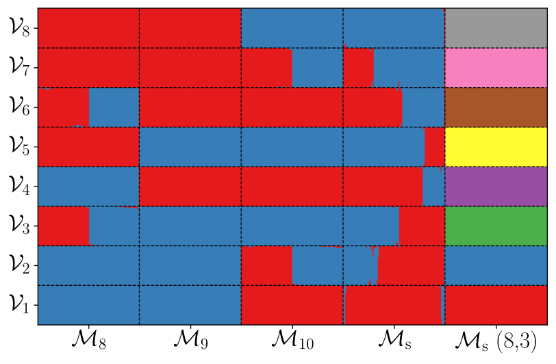
Appendix E Additional Real World Results

In this section we present additional results for some of our real world experiments.

US-Migration network

Figure 19 plots clusterings obtained from the US-Migration network using all 15 weighted functional motifs. Note how the different motifs uncover a variety of different clusterings, and also that they all display good spatial coherence. For completeness, Figure 20 shows the equivalent plots for structural motifs. Note that motifs $\mathcal{M}_{\mathrm{d}}$ and $\mathcal{M}_{4}$ are bi-directional cliques on two and three vertices respectively, so their functional and structural MAMs are identical. The spatial coherence deteriorates for certain structural motifs, and cluster sizes are occasionally less balanced. We believe this is to do with the high local density of the migration network, preventing some motifs from appearing as structural instances in certain places (see Section 4.4 for another example of structural motifs exhibiting this filtering property, which may or may not be desirable, depending on the application). Note that this effect is most pronounced for the motifs containing single edges (i.e. excluding $\mathcal{M}_{\mathrm{d}}$, $\mathcal{M}_{4}$ and $\mathcal{M}_{13}$), because structural instances of single edges require an edge in precisely one direction, filtering out pairs of nodes which exhibit either no mutual migration or bi-directional mutual migration.

Figure 19: Weighted functional motif-based clusterings of the US-Migration network, for all motifs on at most three nodes. Each county (node) is colored by its cluster allocation.

Figure 20: Weighted structural motif-based clusterings of the US-Migration network, for all motifs on at most three nodes. Each county (node) is colored by its cluster allocation.

References

- Adamic and Glance (2005) Adamic LA, Glance N (2005) The political blogosphere and the 2004 US election: Divided they blog. In: Proc. of the 3rd Intl. Workshop on Link Discovery, ACM, New York, pp 36–43
- Ahmed et al (2015) Ahmed NK, Neville J, Rossi RA, Duffield N (2015) Efficient graphlet counting for large networks. In: 2015 IEEE International Conference on Data Mining, IEEE, New York, pp 1–10
- Aicher et al (2013) Aicher C, Jacobs AZ, Clauset A (2013) Adapting the stochastic block model to edge-weighted networks,. arXiv preprint arXiv:1305.5782. Accessed 11 Feb 2020
- Aicher et al (2014) Aicher C, Jacobs AZ, Clauset A (2014) Learning latent block structure in weighted networks. Journal of Complex Networks 3(2):221–248, DOI 10.1093/comnet/cnu026
- Albert (2005) Albert R (2005) Scale-free networks in cell biology. Journal of Cell Science 118(21):4947–4957
- Arthur and Vassilvitskii (2007) Arthur D, Vassilvitskii S (2007) -means++: The advantages of careful seeding. In: Proceedings of the Eighteenth Annual ACM-SIAM Symposium on Discrete Algorithms, SIAM, Philadelphia, pp 1027–1035
- Barabási and Albert (1999) Barabási AL, Albert R (1999) Emergence of scaling in random networks. Science 286(5439):509–512
- Benson et al (2016) Benson AR, Gleich DF, Leskovec J (2016) Higher-order organization of complex networks. Science 353(6295):163–166
- Benson et al (2018) Benson AR, Abebe R, Schaub MT, Jadbabaie A, Kleinberg J (2018) Simplicial closure and higher-order link prediction. Proceedings of the National Academy of Sciences 115(48):E11,221–E11,230, DOI 10.1073/pnas.1800683115
- Cheeger (1969) Cheeger J (1969) A lower bound for the smallest eigenvalue of the Laplacian. In: Proceedings of the Princeton Conference in Honor of Professor S. Bochner, Princeton University Press, Princeton
- Chessa et al (2014) Chessa A, Crimaldi I, Riccaboni M, Trapin L (2014) Cluster analysis of weighted bipartite networks: a new copula-based approach. PLOS ONE 9(10):1–12
- Chung (2005) Chung F (2005) Laplacians and the Cheeger inequality for directed graphs. Annals of Combinatorics 9(1):1–19
- Clauset et al (2007) Clauset A, Tucker E, Sainz M (2007) Filmtipset user movie ratings. The Colorado Index of Complex Networks. https://icon.colorado.edu/, accessed 15 Apr 2019
- Cucuringu (2016) Cucuringu M (2016) Sync-rank: Robust ranking, constrained ranking and rank aggregation via eigenvector and SDP synchronization. IEEE Transactions on Network Science and Engineering 3(1):58–79
- Cucuringu et al (2019a) Cucuringu M, Davies P, Glielmo A, Tyagi H (2019a) SPONGE: A generalized eigenproblem for clustering signed networks. In: Proceedings of Machine Learning Research, PMLR, online, Proceedings of Machine Learning Research, vol 89, pp 1088–1098
- Cucuringu et al (2019b) Cucuringu M, Li H, Sun H, Zanetti L (2019b) Hermitian matrices for clustering directed graphs: insights and applications,. arXiv preprint arXiv:1908.02096. Accessed 19 Feb 2020
- Demeyer et al (2013) Demeyer S, Michoel T, Fostier J, Audenaert P, Pickavet M, Demeester P (2013) The index-based subgraph matching algorithm (ISMA): Fast subgraph enumeration in large networks using optimized search trees. PLOS ONE 8(4):1–15, DOI 10.1371/journal.pone.0061183
- Donath and Hoffman (1972) Donath WE, Hoffman AJ (1972) Algorithms for partitioning of graphs and computer logic based on eigenvectors of connection matrices. IBM Technical Disclosure Bulletin 15(3):938–944
- Elliott et al (2019a) Elliott A, Chiu A, Bazzi M, Reinert G, Cucuringu M (2019a) Core-periphery structure in directed networks,. arXiv preprint arXiv:1912.00984. Accessed 22 Mar 2020
- Elliott et al (2019b) Elliott A, Cucuringu M, Luaces MM, Reidy P, Reinert G (2019b) Anomaly detection in networks with application to financial transaction networks,. arXiv preprint arXiv:1901.00402. Accessed 22 Mar 2020
- Erdős et al (1959) Erdős P, Rényi A, et al (1959) On random graphs. Publicationes Mathematicae 6(26):290–297
- Florescu and Perkins (2016) Florescu L, Perkins W (2016) Spectral thresholds in the bipartite stochastic block model. In: 29th Annual Conference on Learning Theory, PMLR, online, vol 49, pp 943–959
- Fortunato (2010) Fortunato S (2010) Community detection in graphs. Physics Reports 486(3-5):75–174
- Fortunato and Hric (2016) Fortunato S, Hric D (2016) Community detection in networks: A user guide. Physics Reports 659:1–44
- Frey and Dueck (2007) Frey BJ, Dueck D (2007) Clustering by passing messages between data points. Science 315(5814):972–976
- GeoNames (2019) GeoNames (2019) GeoNames. https://www.geonames.org/, Creative Commons, Accessed 24 Mar 2019
- Guattery and Miller (1995) Guattery S, Miller GL (1995) On the performance of spectral graph partitioning methods. In: SODA, vol 95, pp 233–242
- Guattery and Miller (1998) Guattery S, Miller GL (1998) On the quality of spectral separators. SIAM Journal on Matrix Analysis and Applications 19(3):701–719
- Huang et al (2019) Huang J, Shen H, Hou L, Cheng X (2019) Signed graph attention networks. In: International Conference on Artificial Neural Networks, Springer, Cham, pp 566–577
- Hubert and Arabie (1985) Hubert L, Arabie P (1985) Comparing partitions. Journal of Classification 2(1):193–218
- Jacob and Lapkin (2018) Jacob PM, Lapkin A (2018) Statistics of the network of organic chemistry. Reaction Chemistry & Engineering 3(1):102–118
- Joseph et al (2016) Joseph A, Yu B, et al (2016) Impact of regularization on spectral clustering. The Annals of Statistics 44(4):1765–1791
- Karrer and Newman (2011) Karrer B, Newman ME (2011) Stochastic blockmodels and community structure in networks. Physical Review E 83(1):016,107
- Kolaczyk and Csárdi (2014) Kolaczyk ED, Csárdi G (2014) Statistical Analysis of Network Data with R, vol 65. Springer, New York
- KONECT: The Koblenz Network Collection (2019) KONECT: The Koblenz Network Collection (2019) Unicode Languages network dataset. http://konect.cc/networks/unicodelang, accessed 24 Mar 2019
- Leskovec and Krevl (2007) Leskovec J, Krevl A (2007) Astrophysics collaboration network, SNAP Datasets: Stanford large network dataset collection. http://snap.stanford.edu/data/ca-AstroPh.html, accessed 15 Apr 2019
- Leskovec and Krevl (2014) Leskovec J, Krevl A (2014) SNAP Datasets: Stanford large network dataset collection. http://snap.stanford.edu/data, accessed 21 Mar 2020
- Li (2017) Li GX (2017) Divided we tweet: Community detection in political networks. Final Report, Bachelor of Science in Engineering, Department of Engineering, Princeton University
- Li and Milenkovic (2017) Li P, Milenkovic O (2017) Inhomogeneous hypergraph clustering with applications. In: Advances in Neural Information Processing Systems, Curran Associates, Inc., New York, pp 2308–2318
- Li and Milenkovic (2018) Li P, Milenkovic O (2018) Submodular hypergraphs: p-laplacians, Cheeger inequalities and spectral clustering,. arXiv preprint arXiv:1803.03833. Accessed 24 Jun 2020
- Li et al (2016) Li P, Dau H, Puleo G, Milenkovic O (2016) Motif clustering and overlapping clustering for social network analysis,. arXiv preprint arXiv:1612.00895
- Lütkepohl (1996) Lütkepohl H (1996) Handbook of Matrices, vol 1. Wiley, Chichester
- Mangan and Alon (2003) Mangan S, Alon U (2003) Structure and function of the feed-forward loop network motif. Proceedings of the National Academy of Sciences 100(21):11,980–11,985, DOI 10.1073/pnas.2133841100
- Mariadassou et al (2010) Mariadassou M, Robin S, Vacher C, et al (2010) Uncovering latent structure in valued graphs: a variational approach. The Annals of Applied Statistics 4(2):715–742
- Meilă and Pentney (2007) Meilă M, Pentney W (2007) Clustering by weighted cuts in directed graphs. In: Proceedings of the 2007 SIAM international conference on data mining, SIAM, Philadelphia, pp 135–144
- Monti et al (2018) Monti F, Otness K, Bronstein MM (2018) Motifnet: a motif-based graph convolutional network for directed graphs,. arXiv preprint arXiv:1802.01572. Accessed 22 Mar 2020
- Mora et al (2018) Mora BB, Cirtwill AR, Stouffer DB (2018) pymfinder: a tool for the motif analysis of binary and quantitative complex networks. bioRxiv DOI 10.1101/364703
- Nadler et al (2006) Nadler B, Lafon S, Kevrekidis I, Coifman RR (2006) Diffusion maps, spectral clustering and eigenfunctions of Fokker–Planck operators. In: Advances in Neural Information Processing Systems 18, MIT Press, Cambridge, MA, pp 955–962
- Newman (2008) Newman M (2008) The physics of networks. Physics Today 61(11):33–38
- Newman (2004) Newman ME (2004) Analysis of weighted networks. Physical review E 70(5):056,131
- Nguyen et al (2009) Nguyen V, Epps J, Bailey J (2009) Information theoretic measures for clusterings comparison: is a correction for chance necessary? In: International Conference on Machine Learning 2009, ACM, New York, pp 1073–1080
- Nowicki and Snijders (2001) Nowicki K, Snijders TAB (2001) Estimation and prediction for stochastic blockstructures. Journal of the American Statistical Association 96(455):1077–1087
- Onnela et al (2005) Onnela JP, Saramäki J, Kertész J, Kaski K (2005) Intensity and coherence of motifs in weighted complex networks. Physical Review E 71(6):065,103
- Pashanasangi and Seshadhri (2020) Pashanasangi N, Seshadhri C (2020) Efficiently counting vertex orbits of all 5-vertex subgraphs, by EVOKE. In: Proceedings of the 13th International Conference on Web Search and Data Mining, ACM, New York, pp 447–455
- Qin and Rohe (2013) Qin T, Rohe K (2013) Regularized spectral clustering under the degree-corrected stochastic blockmodel. In: Advances in Neural Information Processing Systems 26, Curran Associates, Inc., New York, pp 3120–3128
- Rand (1971) Rand WM (1971) Objective criteria for the evaluation of clustering methods. Journal of the American Statistical Association 66(336):846–850
- Rohe et al (2016) Rohe K, Qin T, Yu B (2016) Co-clustering directed graphs to discover asymmetries and directional communities. Proceedings of the National Academy of Sciences 113(45):12,679–12,684
- Rosvall et al (2014) Rosvall M, Esquivel AV, Lancichinetti A, West JD, Lambiotte R (2014) Memory in network flows and its effects on spreading dynamics and community detection. Nature Communications 5(1):1–13
- Satuluri and Parthasarathy (2011) Satuluri V, Parthasarathy S (2011) Symmetrizations for clustering directed graphs. In: Proceedings of the 14th International Conference on Extending Database Technology, ACM, New York, pp 343–354
- Schaeffer (2007) Schaeffer SE (2007) Graph clustering. Computer Science Review 1(1):27–64
- Shi and Malik (2000) Shi J, Malik J (2000) Normalized cuts and image segmentation. Departmental Papers (CIS) pp 888–905
- Simmons et al (2019) Simmons BI, Sweering MJM, Schillinger M, Dicks LV, Sutherland WJ, Clemente RD (2019) bmotif: A package for motif analyses of bipartite networks. Methods in Ecology and Evolution DOI 10.1111/2041-210X.13149
- Stewart, G.W. and Sun, Ji-guang (1990) Stewart, GW and Sun, Ji-guang (1990) Matrix Perturbation Theory. Academic Press, Boston
- Stram et al (2017) Stram R, Reuss P, Althoff KD (2017) Weighted one mode projection of a bipartite graph as a local similarity measure. In: International Conference on Case-Based Reasoning, Springer, Cham, pp 375–389
- Strassen (1969) Strassen V (1969) Gaussian elimination is not optimal. Numerische Mathematik 13(4):354–356
- Tsourakakis et al (2017) Tsourakakis CE, Pachocki J, Mitzenmacher M (2017) Scalable motif-aware graph clustering. In: Proceedings of the 26th International Conference on World Wide Web, International World Wide Web Conferences Steering Committee, Geneva, pp 1451–1460
- U.S. Census Bureau (2002) US Census Bureau (2002) County-to-county migration flow files. https://www.census.gov/population/www/cen2000/ctytoctyflow/index.html, accessed 02 Mar 2019
- U.S. Census Bureau (2003) US Census Bureau (2003) Domestic migration across regions, divisions, and states: 1995 to 2000. https://www.census.gov/population/www/cen2000/migration, Cenus 2000 Special Reports. Accessed 27 Jun 2020
- Veldt et al (2020) Veldt N, Benson AR, Kleinberg J (2020) Minimizing localized ratio cut objectives in hypergraphs,. arXiv preprint arXiv:1901.00402. Accessed 06 Jul 2020
- Von Luxburg (2007) Von Luxburg U (2007) A tutorial on spectral clustering. Statistics and Computing 17(4):395–416
- Von Luxburg et al (2004) Von Luxburg U, Bousquet O, Belkin M (2004) On the convergence of spectral clustering on random samples: The normalized case. In: Learning Theory, Springer, Berlin, Heidelburg, pp 457–471
- Wagner and Wagner (1993) Wagner D, Wagner F (1993) Between min cut and graph bisection. In: International Symposium on Mathematical Foundations of Computer Science, Springer, Berlin, Heidelburg, pp 744–750
- Wang et al (2018) Wang Y, Wang H, Zhang S (2018) A weighted higher-order network analysis of fine particulate matter (PM2.5) transport in Yangtze River Delta. Physica A: Statistical Mechanics and its Applications 496:654–662
- Wasserman et al (1994) Wasserman S, Faust K, et al (1994) Social network analysis: Methods and applications, vol 8. Cambridge University Press, Cambridge
- Wegner et al (2018) Wegner AE, Ospina-Forero L, Gaunt RE, Deane CM, Reinert G (2018) Identifying networks with common organizational principles. Journal of Complex Networks 6(6):887–913, DOI 10.1093/comnet/cny003
- Wernicke (2006) Wernicke S (2006) Efficient detection of network motifs. IEEE/ACM Transactions on Computational Biology and Bioinformatics (TCBB) 3(4):347–359, DOI 10.1109/TCBB.2006.51
- Wernicke and Rasche (2006) Wernicke S, Rasche F (2006) FANMOD: A tool for fast network motif detection. Bioinformatics 22(9):1152–1153
- Yin et al (2017) Yin H, Benson AR, Leskovec J, Gleich DF (2017) Local higher-order graph clustering. In: Proceedings of the 23rd ACM SIGKDD International Conference on Knowledge Discovery and Data Mining, ACM, New York, pp 555–564
- Zha et al (2001) Zha H, He X, Ding C, Simon H, Gu M (2001) Bipartite graph partitioning and data clustering. In: Proceedings of the tenth international conference on information and knowledge management, ACM, New York, pp 25–32
- Zhang and Rohe (2018) Zhang Y, Rohe K (2018) Understanding regularized spectral clustering via graph conductance. In: Advances in Neural Information Processing Systems, Curran Associates, Inc., New York, pp 10,631–10,640