A Quadratic Program based Control Synthesis under Spatiotemporal Constraints and Non-vanishing Disturbances

Abstract

In this paper, we study the effect of non-vanishing disturbances on the stability of fixed-time stable (FxTS) systems. We present a new result on FxTS, which allows a positive term in the time derivative of the Lyapunov function with the aim to model bounded, non-vanishing disturbances in the system dynamics. We characterize the neighborhood to which the system trajectories converge, as well the time of convergence to this neighborhood, in terms of the positive and negative terms that appear in the time derivative of the Lyapunov function. Then, we use the new FxTS result and formulate a quadratic program (QP) that yields control inputs which drive the trajectories of a class of nonlinear, control-affine systems to a goal set in the presence of control input constraints and non-vanishing, bounded disturbances in the system dynamics. We consider an overtaking problem on a highway as a case study, and discuss how to setup the QP for the considered problem, and how to make a decision on when to start the overtake maneuver, in the presence of sensing errors.

I Introduction

Control design for systems with input and state constraints is not a trivial task. Spatio-temporal specifications typically impose spatial constraints that require the system trajectories to be in a safe set at all times, and temporal constraints that impose convergence of the system trajectories to a goal set within a given time. Incorporating safety related constraints on the system states can be achieved via control barrier functions (CBF) [1]. For requirements involving convergence of the system states to a desired location or a set, approaches using control Lyapunov functions (CLF) [2, 3, 4] are very popular. Many authors have used CLFs in control design either via Sontag’s formula [5, 6], or in an optimization framework [7, 2] to guarantee convergence of closed-loop system trajectories to a given goal point or a goal set.

For concurrent safety and convergence guarantees, a combination of CLFs and CBFs in the control synthesis can be used [1, 5], where the CLF guarantees convergence while the CBF guarantees safety of the state trajectories. The authors in [8] utilize Lyapunov-like barrier functions to guarantee asymptotic tracking of a time-varying output trajectory, while the system output always remains inside a given set. Casting control synthesis problems as quadratic programs has gained popularity recently due to ease of implementation on real-time systems [9, 10]. The fact that CLF and CBF conditions are linear in the control input enables the use of QPs for problems involving spatiotemporal specifications [2, 3, 1]. The authors in [11] use CBFs to encode signal-temporal logic (STL) specifications and formulate a QP to compute the control input. It is worth noticing that most of the aforementioned work is concerned with designing control laws so that reaching a desired location or a desired goal set is achieved as time goes to infinity, i.e., asymptotically.

Based on the notion of fixed-time stability (FxTS) [12], the authors in [13] define a Fixed-Time CLF to guarantee convergence of the state trajectories to the origin within a fixed time, as opposed to asymptotic or exponential convergence. From a practical point of view, it is also important to consider and design robust controllers against uncertainties and disturbances in the system dynamics to account for unmodeled dynamics and sensing errors. Robust CBFs guarantee forward-invariance of safe sets [9, 14, 15]. Typically, the safe set is contracted by a small amount that depends upon the Lipschitz constants of the CBF and the bound on the considered disturbance.

In the presence of non-vanishing disturbances, typically only boundedness of the trajectories in a neighborhood of the nominal equilibrium (or set) can be guaranteed (see, e.g., [16, Section 9.2]). In this paper, we consider bounded, non-vanishing disturbances in the dynamics of a (nominal) system with a FxTS equilibrium, and guarantee that the system trajectories converge to a neighborhood of the nominal equilibrium point within a fixed time. We characterize the size of this neighborhood and the convergence time as a function of the bound of the considered disturbances. Then, in conjunction with robust CBFs, we formulate a QP to compute a control input that renders the safe set forward invariant, and drives the closed-loop trajectories to a neighborhood of a desired goal set within a fixed time, in the presence of control input constraints. Finally, to demonstrate the applicability of the theoretical results, we consider a two-lane overtake scenario where an Ego car is required to overtake a Lead car while maintaining a safe distance from it, within an available time-window dictated by the presence of an Oncoming car in the overtake lane. We assume that the position and the velocity of the other cars are available to the Ego car within some bounded error to model sensing uncertainties, and that the control inputs are subject to some bounded actuation error. Then, utilizing the new robust FxTS result, we formulate a systematic way of deciding for the Ego car whether executing an overtake is safe or not. When safe, the developed QP formulation produces the controller for the Ego car to safely perform the overtake maneuver in the available time frame.

The paper is organized as follows. Section II provides the foundations for Set Invariance and Fixed-Time Stability (FxTS), and introduces preliminary results on Robust FxT CLFs and Robust CBFs. In Section III an overtaking problem is used to motivate the Robust FxT-CLF-CBF-QP framework, while Section IV discusses the simulation results. We end with conclusion and directions for future work in Section V.

II Mathematical Preliminaries

In the rest of the paper, $\mathbb{R}$ denotes the set of real numbers and $\mathbb{R}_{+}$ denotes the set of non-negative real numbers. We use $\|\cdot\|$ to denote the Euclidean norm. We write $\partial S$ for the boundary of the closed set $S$, $\textrm{int}(S)$ for its interior. The Lie derivative of a function $V:\mathbb{R}^{n}\rightarrow\mathbb{R}$ along a vector field $f:\mathbb{R}^{n}\rightarrow\mathbb{R}^{n}$ at a point $x\in\mathbb{R}^{n}$ is denoted as $L_{f}V(x)\triangleq\frac{\partial V}{\partial x}f(x)$.

II-A Forward Invariance of Safe Set

Consider the control affine system

$$\dot{x}(t) =f(x(t))+g(x(t))u(t),\quad x(t_{0})=x_{0},$$ (1)

where $x\in\mathbb{R}^{n}$, $u\in\mathcal{U}\subset\mathbb{R}^{m}$ are the state and the control input vector, respectively, $f:\mathbb{R}^{n}\rightarrow\mathbb{R}^{n}$ and $g:\mathbb{R}^{n}\rightarrow\mathbb{R}^{n\times m}$ are continuous functions. Here, $\mathcal{U}$ denotes the set of admissible control inputs. Define a safe set $S_{s}=\{x\;|\;h_{s}(x)\geq 0\}$, and consider a goal set to be reached in a prescribed time $T$ defined as $S_{G}=\{x\;|\;h_{g}(x)\leq 0\}$, where $h_{s},h_{g}:\mathbb{R}^{n}\rightarrow\mathbb{R}$ are continuously differentiable functions.

We present a necessary and sufficient condition, known as Nagumo’s Theorem, for guaranteeing forward invariance of the safe set $S_{s}$, i.e., safety of the system trajectories.

Lemma 1.

Let the solution of the (1) exist and be unique in forward time. Then, the set $S_{s}$ is forward-invariant for the closed-loop trajectories of (1) with $x(0)\in S_{s}$ if and only there exists a control input $u\in\mathcal{U}$ such that $L_{f}h_{s}(x)+L_{g}h_{s}(x)u\geq 0$ for all $x\in\partial S_{s}$, where $\partial S_{s}\triangleq\{x\;|\;h_{s}(x)=0\}$ is the boundary of the safe set $S_{s}$.

II-B Fixed-Time Stability

Next, we review the notion of fixed-time stability. Consider the nonlinear system

$$\dot{x}(t)=f(x(t)),\quad x(0)=x_{0},$$ (2)

where $x\in\mathbb{R}^{n}$ and $f:\mathbb{R}^{n}\rightarrow\mathbb{R}^{n}$ is continuous with $f(0)=0$. The origin is said to be an FxTS equilibrium of (2) if it is Lyapunov stable and fixed-time convergent, i.e., for all $x(0)\in\mathbb{R}^{n}$, the system trajectories satisfy $\lim_{t\to T}x(t)=0$, where $T<\infty$ is independent of $x(0)$ [12]. Lyapunov conditions for FxTS is given as follows.

Theorem 1 ([12]).

Suppose there exists a positive definite function $V:\mathbb{R}^{n}\rightarrow\mathbb{R}$ such that

$$\dot{V}(x)\leq-aV(x)^{p}-bV(x)^{q},$$ (3)

holds along the trajectories of (2) with $a,b>0$, $0<p<1$ and $q>1$. Then, the origin of (2) is FxTS with a settling time $T\leq T_{b}$ where

$$T_{b}\leq\frac{1}{a(1-p)}+\frac{1}{b(q-1)}.$$ (4)

We need the following lemma to prove one of the main results of the paper.

Lemma 2.

Let $V_{0},c_{1},c_{2}>0,c_{3}>0$, $a_{1}=1+\frac{1}{\mu}$ and $a_{2}=1-\frac{1}{\mu}$, where $\mu>1$. Define

$$I\triangleq\int_{V_{0}}^{\bar{V}}\frac{dV}{-c_{1}V^{a_{1}}-c_{2}V^{a_{2}}+c_{3}}.$$ (5)

Then, the following holds:

• If $c_{3}<2\sqrt{c_{1}c_{2}}$, we have for all $V_{0}\geq\bar{V}=1$

  $$I\leq\frac{\mu}{c_{1}k_{1}}\left(\frac{\pi}{2}-\tan^{-1}k_{2}\right),$$ (6)

  where $k_{1}=\sqrt{\frac{4c_{1}c_{2}-c_{3}^{2}}{4c_{1}^{2}}}$ and $k_{2}=\frac{2c_{1}-c_{3}}{\sqrt{4c_{1}c_{2}-c_{3}^{2}}}$;

• If $c_{3}\geq 2\sqrt{c_{1}c_{2}}$ and $V_{0}\geq\bar{V}=k\Big(\frac{c_{3}+\sqrt{c_{3}^{2}-4c_{1}c_{2}}}{2c_{1}}\Big)^{\mu}$ with $k>1$, we have for all $V_{0}\geq\bar{V}$

  $$I \leq\frac{\mu}{c_{1}(b-a)}\log\left(\frac{kb-b}{kb-a}\right),$$

  where $a,b$ are the roots of $\gamma(z)\triangleq c_{1}z^{2}-c_{3}z+c_{2}=0$;

The proof is provided in Appendix A.

Building upon the nominal system (1), we now consider the perturbed system, given as

$$\dot{x}(t)=f(x(t))+g(x(t))u(t)+\phi(x(t)),\quad x(0)=x_{0}$$ (7)

where $f,g$ are as in (1), and $\phi:\mathbb{R}^{n}\rightarrow\mathbb{R}^{n}$ is an added, unmatched disturbance, possibly non-vanishing, which is assumed to be bounded. We denote the upper bound as $\|\phi\|_{\infty}\triangleq\sup_{x\in\mathcal{D}_{0}}\|\phi(x)\|$, where $\mathcal{D}_{0}\subseteq\mathbb{R}^{n}$ is a neighborhood of the origin. The added disturbance $\phi$ models uncertainties in the parameters used in the control design; external perturbations to the dynamics, such as wind; and actuation errors, for example a power surge. Although uncertainty in a system can be treated in several different ways (see, e.g., [15], [17]), we will restrict our focus to systems of the form (7). Next, we present a new result on robustness of the trajectories around nominal FxTS equilibria against a class of bounded, non-vanishing disturbances.

II-C Robust FxT CLF

We extend the result in Theorem 1 by introducing a positive constant in the upper bound of the time derivative of the Lyapunov candidate, $V$. We refer to $V$ as a robust FxT-CLF and .

Theorem 2.

Let $V:\mathbb{R}^{n}\rightarrow\mathbb{R}$ be a continuously differentiable, positive definite, proper function, satisfying

$$\dot{V}\leq-c_{1}V^{a_{1}}-c_{2}V^{a_{2}}+c_{3},$$ (8)

with $c_{1},c_{2}>0$, $c_{3}\in\mathbb{R}$, $a_{1}=1+\frac{1}{\mu}$, $a_{2}=1-\frac{1}{\mu}$ for some $\mu>1$, along the trajectories of (2). Then, there exists a neighborhood $D$ of the origin such that for all $x(0)\in\mathbb{R}^{n}\setminus D$, the trajectories of (2) reach $D$ in a fixed time $T$, where

$$D =\begin{cases}\{x\;|\;V(x)\leq k\Big(\frac{c_{3}+\sqrt{c_{3}^{2}-4c_{1}c_{2}}}{2c_{1}}\Big)^{\mu}\};&c_{3}\geq 2\sqrt{c_{1}c_{2}},\\ \{x\;|\;V(x)\leq\frac{c_{3}}{2\sqrt{c_{1}c_{2}}}\},&0<c_{3}<2\sqrt{c_{1}c_{2}},\\ \{0\},&c_{3}\leq 0,\end{cases},$$ (9)

$$T \leq\begin{cases}\frac{\mu}{c_{1}(b-a)}\log\left(\frac{kb-b}{kb-a}\right);&c_{3}\geq 2\sqrt{c_{1}c_{2}},\\ \frac{\mu}{c_{1}k_{1}}\left(\frac{\pi}{2}-\tan^{-1}k_{2}\right),&0<c_{3}<2\sqrt{c_{1}c_{2}},\\ \frac{\mu\pi}{2\sqrt{c_{1}c_{2}}},&c_{3}\leq 0,\end{cases},$$ (10)

where $k>1$, $a,b$ are the solutions of $\gamma(s)=c_{1}s^{2}-c_{3}s+c_{2}=0$, $k_{1}=\sqrt{\frac{4c_{1}c_{2}-c_{3}^{2}}{4c_{1}^{2}}}$, and $k_{2}=-\frac{c_{3}}{\sqrt{4c_{1}c_{2}-c_{3}^{2}}}$.

Proof.

Note that for $c_{3}\leq 0$, we obtain (3) from (8), and so FxTS of the origin is guaranteed for all $x\in\mathbb{R}^{n}$. Thus, we concentrate on the case when $c_{3}>0$, for which sufficiently small values of $V$ cause the right hand side of (8) to become positive. The proof follows from Lemma 2. Consider (8) and let $c_{1}V^{a_{1}}+c_{2}V^{a_{2}}>c_{3}$. Re-write the inequality to obtain

$$\int_{V_{0}}^{V(x(T))}\frac{1}{-c_{1}V^{a_{1}}-c_{2}V^{a_{2}}+c_{3}}dV\geq\int_{0}^{T}dt=T,$$ (11)

where $V_{0}=V(x(0))$ and $T$ is the time when the system trajectories first reach the domain $D$. It is easy to show that for each of the cases listed in the Theorem statement, $c_{1}V^{a_{1}}+c_{2}V^{a_{2}}>c_{3}$ and thus the right-hand side of (8) is negative for all $x\notin D$. Now, to show that the system trajectories converge to $D$ in fixed-time, we compute upper bounds on $T$.

For the case when $c_{3}<2\sqrt{c_{1}c_{2}}$, part (i) in Lemma 2 provides an upper bound on the left-hand side of (11) for $x\notin D=\{x\;|\;V(x)\leq\frac{c_{3}}{2\sqrt{c_{1}c_{2}}}\}$. Similarly, for the case $c_{3}\geq 2\sqrt{c_{1}c_{2}}$, part (ii) of Lemma 2 provides upper bounds on the left-hand side of (11). Thus, we obtain the domains $D$ and the bounds on convergence times $T$ for the various cases directly from Lemma 2. Since for all three cases, $T<\infty$ and is independent of the initial conditions, we have that the system trajectories reach the set $D$ within a fixed time $T$. ∎

Next, we use Theorem 2 to show robustness of a FxTS origin against a class of non-vanishing, bounded, additive disturbance in the system dynamics.

Corollary 1.

Assume that there exists $u(t)\in\mathcal{U}$, where $\mathcal{U}$ is a set of admissible control inputs, such that the origin for the nominal system (1) is fixed-time stable, and that there exists a Lyapunov function $V$ satisfying conditions of Theorem 1. Additionally, assume that there exists $L>0$ such that $\left\|\frac{\partial V}{\partial x}\right\|\leq L$ for all $x\in\mathcal{D}_{0}\subseteq\mathbb{R}^{n}$. Then, there exists $D\subset\mathbb{R}^{n}$ such that for all $x(0)\in\mathcal{D}_{0}\setminus D$, the trajectories of (7) reach the set $D$ in a fixed time.

Proof.

The time derivative of $V$ along the system trajectories of (7) reads

$$\dot{V}=\frac{\partial V}{\partial x}[f(x)+g(x)u+\phi(x)]\leq -aV^{p}-bV^{q}+L\|\phi\|_{\infty}.$$

Hence, using Theorem 2, we obtain that there exists $D\subset\mathbb{R}^{n}$ such that all solutions starting outside $D$ reach the set $D$ in a fixed time $T$, where the set $D$ and the convergence time $T$ is a function of $a,b,p,q,L$ and $\|\phi\|_{\infty}$. ∎

Note that in the presence of non-vanishing disturbances, it is not possible to guarantee that the system trajectories converge to the equilibrium point. Instead, (9) characterizes an estimate, $D$, of a neighborhood of the equilibrium to where system trajectories are guaranteed to converge within a fixed-time, $T$, and (10) provides an upper bound independent of $x(0)\in D$ on $T$. We observe that although this result shares commonalities with the notion of Input-to-State Stability [18], it is both more restrictive on $\dot{V}$ and allows us to explicitly characterize $D$ and $T$.

II-D Robust CBF

Next, we review the notion of a robust CBF, to guarantee forward invariance of a safe set, in the presence of a class of additive, non-vanishing disturbances. Here, we assume that $S_{s}\subset\mathcal{D}_{0}$.

Lemma 3.

The set $S_{s}$ is forward-invariant for the closed-loop trajectories of (7) if

$$\inf_{u\in\mathcal{U}}\{L_{f}h_{s}(x)+L_{g}h_{s}(x)u\}\geq-\left\|\frac{\partial h_{s}(x)}{\partial x}\right\|\|\phi\|_{\infty},$$ (12)

holds for all $x\in\partial S_{s}\cap\mathcal{D}_{0}$.

Proof.

The time derivative of $h_{s}$ along the trajectories of (7) reads

$$\dot{h}_{s}=L_{f}h_{s}(x)+L_{g}h_{s}(x)u+\frac{\partial h_{s}(x)}{\partial x}\phi(x).$$

For $x\in\partial S_{s}\cap\mathcal{D}_{0}$, we have that $h_{s}(x)=0$ and $\|\phi(x)\|\leq\|\phi\|_{\infty}$. Using (12), we obtain that there exists a $u\in\mathcal{U}$ such that $\dot{h}_{s}\geq 0$. Thus, using Lemma 1, we have that forward invariance of set $S$ is guaranteed. ∎

Thus, condition (12), which notably need only hold at the boundary of a safe set, $S_{s}$, can be used to guarantee forward invariance of such a set in the presence of a class of additive, non-vanishing disturbances. Next, we take up a case study, and discuss how we can use the robust FxT-CLF and robust CBF in a QP framework to compute a control input so that the conditions (8), (12) hold along the closed-loop trajectories.

III Case study: Overtake Problem

In this section, we introduce a framework for computing overtake control via a FxT-CLF-CBF QP subject to bounded, non-vanishing, additive disturbances.

III-A Problem Formulation

We consider an Ego car starting behind a slowly-moving, Lead car on a two-lane undivided highway, where the Ego car seeks to overtake the Lead car in a safe, timely manner whilst avoiding oncoming traffic (see Figure 1). The combined effort to achieve lane-keeping (maintaining the vehicle’s position at the center of the lane), obstacle avoidance (remaining a safe distance between both other vehicles and the road edges), and goal-reaching within a fixed-time, $T$, (completing the overtake) in the presence of input constraints makes this problem challenging.

Fig. 1: Problem setup for the overtake problem. The Ego car seeks to overtake the Lead car safely in the overtaking lane while avoiding a collision with the Oncoming car.

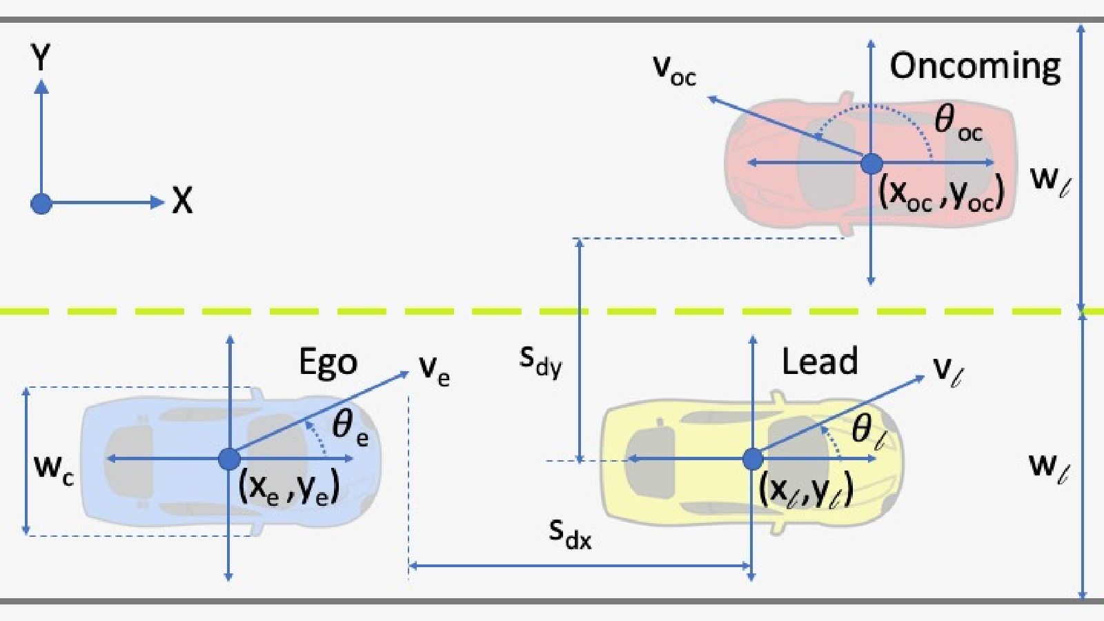
For each vehicle, we select the model of a kinematic bicycle in an inertial frame, introduced in [19] and adapted for automobile highway merging in [20]. We use subscripts $e,l,oc$ to denote the Ego, the Lead and Oncoming car. The motion of the cars is modelled as:

$$\dot{q}_{i}=\begin{bmatrix}v_{i}\ \cos(\theta_{i})\\ v_{i}\ \sin(\theta_{i})\\ 0\\ 0\end{bmatrix}+\begin{bmatrix}0&0\\ 0&0\\ 1&0\\ 0&1\end{bmatrix}\begin{bmatrix}\omega_{i}\\ a_{i}\end{bmatrix}+\phi_{i},$$ (13)

where $q_{i}=[x_{i}\ y_{i}\ \theta_{i}\ v_{i}]^{T}$ is the state vector of car $i\in\{e,l,oc\}$, $x_{i}$ is the longitudinal position, $y_{i}$ is the transverse position, $\theta_{i}$ is the heading angle, $v_{i}$ is the velocity, $\omega_{i}$ is the angular control input, and $a_{i}$ is the longitudinal control input (measured as a fraction of $M_{i}g$, where $M_{i}$ is the vehicle mass and $g=9.81$ m/s²). The disturbance in each car’s dynamics, $\phi_{i}$, takes into account modelling error and external perturbations such as wind or road grade. We assume that the disturbance $\phi_{i}$ is bounded, i.e., if $\hat{q}_{l}^{e},\hat{q}_{oc}^{e}$ denote the states of the Lead and Oncoming car as estimated by Ego car, then there exists $\epsilon>0$ such that $\|\hat{q}_{j}^{e}(t)-q_{j}(t)\|\leq\epsilon$ for all $t\geq 0$, $j\in\{l,oc\}$. Consistent with the discussion in the previous section, we define $\|\phi\|_{\infty}=\epsilon$.

The control input $u_{i}\in\mathbb{R}^{2}$ for car $i$ consists of $\omega_{i}$ and $a_{i}$. Notably, our adjustment to the dynamics of [19] is such that $\theta$ describes the full steering dynamics, $\theta=\frac{v\tan(\beta)}{l_{v}}$, where $\beta$ is the steering angle in rad and $l_{v}$ is the length of the vehicle in m. This is a reasonable modification due to the small angle approximation, which we expect to hold in our overtaking problem, and from which we obtain that $tan(\beta)\approx\beta$, such that $\theta\approx\frac{v\beta}{l_{v}}$. Additionally, the vehicles are assumed to obey the no-slip condition imposed by the kinematic bicycle model, and their volumes are taken into consideration when evaluating safety.

The overtake problem considered in the case study is formally stated below.

Problem 1.

Given $q_{e}(0),q_{l}(0),q_{oc}(0)$ determine if overtaking the Lead car is safe, i.e., if there exist vehicle state and control trajectories, $q_{e}(t),q_{l}(t),q_{oc}(t),u_{e}(t)$, where $u_{e}(t)\in\mathcal{U}=\{(\omega,a)\;|\;\omega_{m}\leq\omega\leq\omega_{M},a_{m}\leq a\leq a_{M}\}$, such that $\|x_{e}(t)-x_{i}(t)\|>s_{dx},\|y_{e}(t)-y_{i}(t)\|>s_{dy}$ for $i\in\{l,oc\}$ and $t\in[0,T]$, where $T$ is the upper bound on time required to complete the overtake. If safe, design a control input, $u_{e}(t)\in\mathcal{U}$ for all $x_{e}(0)<x_{l}(0)-s_{dx}$, $y_{e}(0)=y_{l}(0)$, $x_{l}(0)<x_{oc}(0)$, $\theta_{e}(0)=\theta_{l}(0)=0$, $\theta_{oc}(0)=\pi$, and $v_{e}(0),v_{l}(0),v_{oc}(0)>0$, so that the closed-loop trajectories of the Ego car overtake the Lead car.

We divide the Problem 1 into the following sub-problems:

1. Determine when an overtake is safe to initiate;

2. Steer Ego Vehicle safely into overtaking lane;

3. Advance Ego Vehicle safely past Lead Vehicle;

4. Steer Ego Vehicle safely back into original lane.

Note that lane maintenance can also be modelled as a safety constraint. The following CBFs were designed as such: $h_{s,1}$ encodes that the Ego vehicle maintains all four wheels within the road limits at all times even with bounded steering capabilities, while $h_{s,2}$ encodes that the Ego vehicle maintain a safe distance from the Lead Vehicle, as defined by the ellipse centered on the Lead Vehicle with semi-major axes $s_{dx}$ and $s_{dy}$ for the $x$ and $y$ coordinates respectively. The CBFs $h_{s,i}(q)$ were defined as follows:

$$h_{s,1} =(y_{e}-e_{1})(y_{e}-e_{2})$$ (14)

$$h_{s,2} =1-(\frac{x_{l}-x_{e}}{s_{dx}})^{2}-(\frac{y_{l}-y_{e}}{s_{dy}})^{2}$$ (15)

where $s_{dx}=v_{e}\tau\cos{\theta_{e}}+l_{c}$, $s_{dy}=w_{l}-\frac{w_{c}}{2}$, and $e_{1}$, $e_{2}$ are parameters which define the safety barrier at the edge of the road in the $y$ coordinate. Here, $\tau=1.8$ sec is the time headway. Specifically, we define $e_{1}=(\frac{w_{c}}{2})+v_{e}\omega_{max}\left(1-\cos{\theta_{e}}\right)$, and $e_{2}=(2w_{l}-\frac{w_{c}}{2})-v_{e}\omega_{max}\left(1-\cos{\theta_{e}}\right)$, where $w_{l}=3$m is the width of a lane and $w_{c}=2.27$m and $l_{c}=5.05$m are the width and length of a car.

To capture the convergence requirement in each of the sub-problems 2) – 4), we define goal sets $S_{G_{j}}=\{q\;|\;V(q-q_{j}^{g})\leq 0\}$, where $q_{j}^{g}=[x_{j}^{g}\;y_{j}^{g}\;\theta_{j}^{g}\;v_{j}^{g}]^{T}$ denotes the goal location for the $j-th$ sub-problem, $j\in\{2,3,4\}$, and we define $\bar{q}_{j}=q-q_{j}^{g}$. We use a CLF $V:\mathbb{R}^{4}\rightarrow\mathbb{R}$ to encode the convergence requirement, defined as

$$\begin{split}V(\bar{q})=&K(k_{x}\bar{x}^{2}+k_{v}\bar{v}^{2}+k_{xv}\bar{x}\bar{v}\\ &+k_{y}\bar{y}^{2}+k_{\theta}\bar{\theta}^{2}+k_{y\theta}\bar{y}\bar{\theta}-1)\\ \end{split}$$ (16)

where $K$ is a constant gain selected during our parameter selection phase and $k_{x}$, $k_{y}$, $k_{\theta}$, $k_{v}$ $>0$ are constant gains which influence the size and shape of the goal subspace. For positive definiteness of $V$, we impose that $0<k_{xv}<2\sqrt{k_{x}k_{v}}$ and $0<k_{y\theta}<2\sqrt{k_{y}k_{\theta}}$. Finally, we denote $\bar{x}=x_{e}-x_{j}^{g},\bar{y}=y_{e}-y_{j}^{g},\bar{\theta}=\theta_{e}-\theta_{j}^{g}$ and $\bar{v}=v_{e}-v_{j}^{g}$. Note that the convergence requirement, and thus the CLF $V$, changes for each sub-problem.

Consider the following inequalities.

$$L_{f}h_{s_{1}}(x)+L_{g}h_{s_{1}}(x)u \geq 0,$$ (17)

$$L_{f}h_{s_{2}}(x)+L_{g}h_{s_{2}}(x)u \geq 0,$$ (18)

which when true at the boundary of the sets $S_{s_{1}}$ and $S_{s_{2}}$ guarantee forward invariance of the respective sets. We need the following viability assumption before we can proceed with our main results.

Assumption 1.

There exists a control input $u\in\mathcal{U}$ such that

• for all $q\in\partial S_{s_{1}}\cap\partial S_{S_{2}}$, both (17) and (18) holds;

• for all $q\in\partial S_{s_{1}}$ (respectively, $q\in\partial S_{s_{2}}$, (17) (respectively, (18)) holds.

Furthermore, $S_{G_{j}}\cap S_{s_{1}}\cap S_{s_{2}}\neq\emptyset$, $\forall j\in\{2,3,4\}$.

We will now introduce a QP formulation to solve Problem 1. Consider the QP:

$$\min_{u,\delta_{1},\delta_{2},\delta_{3}}\frac{1}{2}u^{T}u+p_{1}\delta_{1}^{2} +p_{2}\delta_{2}^{2}+p_{3}\delta_{3}^{2}+q_{1}\delta_{1}$$ (19a)

$$\textrm{s.t.}\;A_{u}u \leq b_{u}$$ (19b)

$$L_{f}V(q_{e})+L_{g}V(q_{e})u \leq\delta_{1}-\alpha_{1}\max\{0,V(q_{e})\}^{\gamma_{1}}$$

$$\quad-\alpha_{2}\max\{0,V(q_{e})\}^{\gamma_{2}}$$ (19c)

$$L_{f}h_{s_{1}}(q_{e})+L_{g}h_{s_{1}}(q_{e})u \geq-\delta_{2}h_{s_{1}}(q_{e})$$ (19d)

$$L_{f}h_{s_{2}}(q_{e})+L_{g}h_{s_{2}}(q_{e})u \geq-\delta_{3}h_{s_{2}}(q_{e})$$ (19e)

where (19a), quadratic in the decision variables, models a minimum-norm controller with relaxation variables $\delta_{1}$, $\delta_{2}$, $\delta_{3}$ and $p_{1}$, $p_{2}$, $p_{3}$, $q_{1}$ $\geq 0$, $\gamma_{1}=1+\frac{1}{\mu}$, $\gamma_{2}=1-\frac{1}{\mu}$, where $\mu>1$, and $\alpha_{i}=\frac{\pi\mu}{2T}$ for $i=\{1,2\}$. The constraints, all of which are linear in the decision variables, accomplish the following: (19b) enforces input constraints, (19c) provides the FxT convergence guarantee, and (19d) and (19e) provide safety guarantees. Our formulation, specifically (19c), utilizes the result of Theorem 2 in order to guarantee fixed-time convergence for any $\delta_{1}$. Moreover, we discuss the relationship between this $\delta_{1}$ term and an upper limit on the class of additive, bounded, non-vanishing disturbances considered in Problem 1.

Next, we discuss the feasibility of the QP (19).

Lemma 4.

Under Assumption 1, the QP (19) is feasible for all $q\in(S_{S_{1}}\cap S_{S_{2}})\setminus S_{G}$.

Proof.

Let $q\notin S_{G}$, and consider the three cases $q\in\textnormal{int}(S_{S_{1}})\cap\textnormal{int}(S_{S_{2}})$, $q\in\partial S_{S_{1}}$ and $q\in\partial S_{S_{2}}$, separately.

In the first case, we have that $h_{s_{1}},h_{s_{2}},V\neq 0$. Choose any $u$ that satisfies (19b). With this choice of $u$, one can choose $\delta_{1},\delta_{2},\delta_{3}$ so that (19c)-(19e) hold with equality. This is possible since functions $V,h_{s_{1}},h_{s_{2}}$ are non-zero. Thus, for all $q\in\left(\textnormal{int}(S_{S_{1}})\cap\textnormal{int}(S_{S_{2}})\right)\setminus S_{G}$, there exists a solution to (19). Per Assumption 1, for all $q\in\partial S_{S_{1}}$, there exists a control input $u\in\mathcal{U}$ such that (19d) holds with any $\delta_{2}$ (since $h_{s_{1}}(q)=0$ for $q\in\partial S_{S_{1}}$, the choice of $\delta_{2}$ does not matter). Thus, using any $u$ that satisfies (19d), one can define $\delta_{1}$ and $\delta_{3}$ so that (19c) and (19e) hold with equality. Similarly, one can construct a solution for the case when $q\in\partial S_{S_{2}}$, and $q\in\partial S_{S_{1}}\cap\partial S_{S_{2}}$. Thus, the QP (19) is feasible for all $q\in(S_{S_{1}}\cap S_{S_{2}})\setminus S_{G}$. ∎

We are now ready to present our main result.

Theorem 3.

Let the solution to the QP (19) be denoted as $z^{*}(\cdot)=(u^{*}(\cdot),\delta_{1}^{*}(\cdot),\delta_{2}^{*}(\cdot),\delta_{3}^{*}(\cdot))$. Assume that $\|\phi\|_{\infty}\leq\frac{\delta_{1}^{*}}{\|\frac{\partial V}{\partial q}\|}$ for all $q_{e}$, i.e. $L_{\phi}V\leq\delta_{1}^{*}(q)$. If the solution $z^{*}(\cdot)$ is continuous on $\left(S_{S_{1}}\cap S_{S_{2}}\right)\setminus S_{G}$, then under the effect of the control input $u(q_{e})=u^{*}(q_{e})$, the closed-loop trajectories of (7) reach a neighborhood $D$ of the goal set $S_{g}$ in fixed-time $T$, and satisfy $q_{e}(t)\in S_{S_{1}}\cap S_{S_{2}}$ for all $t\geq 0$, where the neighborhood $D$ and time of convergence are given by (9) and (10), with $c_{1}=\alpha_{1},c_{2}=\alpha_{2}$ and $c_{3}=2\max\delta_{1}^{*}$.

Proof.

The proof for the unperturbed case is immediate. The constraint (19c) ensures that the conditions of Theorem 2 are satisfied and therefore convergence to the neighborhood $D$ is achieved in fixed-time, $T$, for the nominal system $\dot{q}=f(q)+g(q)u$. For the perturbed system, $\dot{q}=f(q)+g(q)u+\phi(q)$, we have that $\dot{V}=L_{f}V+L_{g}Vu+L_{\phi}V\leq-\alpha_{1}V^{\gamma_{1}}-\alpha_{2}V^{\gamma_{2}}+\delta_{1}^{*}$, which may be rewritten as $\dot{V}=L_{f}V+L_{g}Vu\leq-\alpha_{1}V^{\gamma_{1}}-\alpha_{2}V^{\gamma_{2}}+2\max\delta_{1}^{*}$. Thus, we have that the closed-loop trajectories of $\dot{q}=f(q)+g(q)u+\phi(q)$ reach $D$ in fixed-time $T$, given by (9) and (10), respectively, with $c_{1}=\alpha_{1}$, $c_{2}=\alpha_{2}$, $c_{3}=2\max\delta_{1}^{*}$. ∎

Remark 1.

Comparing (19c) and Theorem 2 yields an observation that $\delta_{1}^{*}$ in the solution of (19) is analogous to $c_{3}$ in (8). However, in the context of solving Problem 1, (19) must be point-wise in the state space. It follows, therefore, that by considering $\max\delta_{1}^{*}$ over the solution set of (19) we can use $c_{3}=2\max\delta_{1}^{*}$ to obtain a useful, albeit conservative, estimate for the settling time to a neighborhood, $D$, of the goal set, $S_{g}$.

Remark 2.

This method does not estimate the disturbance term, $\phi$; rather, it determines a tolerable upper bound such that FxTS to a neighborhood $D$ of a goal set $S_{G}$ is preserved, as well as characterizations of $D$ and the convergence time, $T$.

Next, we introduce a method for conditioning the parameters in (19) such that $2\max_{q}\delta_{1}(q)^{*}\leq 2\sqrt{\alpha_{1}\alpha_{2}}$. We then use $c_{3}=2\max_{q}\{\delta_{1}^{*}\}$ to compute a conservative estimate on settling time for the Ego Vehicle during each segment of Problem 1. We use the sum total of these time estimates to compute an unsafe overtaking horizon, i.e. $\left(v_{e}\cos\theta_{e}-\hat{v}_{oc}\cos{\hat{\theta}_{oc}}\right)T_{est}$. If an Oncoming Vehicle is inside of the overtaking horizon (nearer to the Ego Vehicle than the horizon), then the Ego Vehicle does not begin its overtake.

IV Simulation Results and Discussion

IV-A Simulation Parameters

The CLF gains in (16) are fixed as: $k_{x}=\frac{1}{60^{2}}$m^-2, $k_{y}=100$m^-2, $k_{\theta}=400$rad^-2, $k_{v}=1$(m/s)^-2, $k_{xv}=0.05\sqrt{k_{x}k_{v}}=\frac{1}{1200}$m^-2s, $k_{y\theta}=0.5\sqrt{k_{y}k_{\theta}}=100$(rad m)^-1 so that the goal set is defined as $C_{g}$: $\|\bar{x}\|\leq 60$ m, $\|\bar{y}\|\leq 0.1$ m, $\|\bar{\theta}\|\leq 0.05$ rad, $\|\bar{v}\|\leq 1$ m/s. The physical boundaries of the road are set to be $y=0$ and $y=2w_{l}$ respectively. The input constraints are given as $|\omega|\leq\frac{\pi}{18}$ rad and $|a|\leq 0.25g$ ms^-2. We used a time-step of $dt=0.001$ sec. Other simulation parameters are: $\mu=5$, which leads to $\gamma_{1}=1.2$ and $\gamma_{2}=0.8$, as well $p_{1}=1200$, $p_{2}=1$, and $q_{1}=1000$. We define $\theta_{g}=\tan^{-1}(\frac{y_{g}-y_{e}}{x_{g}-x_{e}})$ and set $v_{g}=25$ as soon as it is safe to overtake. The final states of one segment are used as initial states to the subsequent segment.

The following discussion will outline in greater detail the setup for each sub-problem.

IV-A1 Ego Vehicle Identify Opportunity to Perform Overtake

The initial states of the Ego ($q_{e}(0)$), Lead ($q_{l}(0)$), and Oncoming ($q_{oc}(0)$) are chosen as $q_{e}(0)=\begin{bmatrix}-\tau v_{l}(0)&\frac{w_{l}}{2}&0&v_{l}(0)\end{bmatrix}^{T}$, $q_{l}(0)=\begin{bmatrix}\tau v_{l}(0)&\frac{w_{l}}{2}&0&v_{l}(0)\end{bmatrix}^{T}$, and $q_{oc}(0)=\begin{bmatrix}x_{e}(0)+2v_{l}(0)t_{p}&2w_{l}-\frac{w_{l}}{2}&-\pi&25\end{bmatrix}$ where $v_{l}(0)$ and $t_{p}$, the time until the Oncoming Vehicle passes by the Ego Vehicle, are chosen a priori. The goal state, $q_{g}$, is defined as an evolving function of $q_{l}$ where the goal location is chosen as $x_{g}=x_{l}-1.5\tau v_{l}+50$, $y_{g}=y_{l}$, and $v_{g}=v_{l}$ until an overtake maneuver is safe to initiate.

IV-A2 Ego Vehicle Merge into Overtaking Lane

We define $y_{g}$ and $v_{g}$ in this segment as: $y_{g}=y_{l}+w_{l}$, $v_{g}=25$. The upper bound on settling time, $T$, is set to $T=10$ sec.

IV-A3 Ego Vehicle Move a Safe Distance beyond Lead Vehicle

The $x_{g}$ coordinate is modified to be: $x_{g}=x_{l}+1.5\tau v_{l}+50$, and $T=\frac{2\tau v_{l}(0)}{v_{g}-v_{l}(0)}+4$ sec to adjust for an increase in safe following distance at increased initial velocities.

IV-A4 Ego Vehicle Merge back into Original Lane

We set $y_{g}=y_{l}$, and $T=6$sec.

IV-B Results

In accordance with Theorem 2, we desire to choose parameters such that it is guaranteed that $2\max\delta_{1}=c_{3}<2\sqrt{c_{1}c_{2}}$, where $c_{i}=\alpha_{i}=\frac{\pi\mu}{2T}$ for $i\in\{1,2\}$ for our nominal simulation. The initial conditions chosen are $v_{l}(0)=17$ and $t_{p}=2$. Thus, we varied $K$ from $10^{-5}$ to 1, $T$ from 13.15 to 30.65, $\omega_{max}$ from 0.0175 to 14.45, and $a_{max}$ from 0.245 to 245.25. We selected the final values as $K=0.0001$, $T=27.65$, and $u_{max}=[0.1745\;2.45]^{T}$. From Figure 2 we see that while increasing control authority yields a marginal decrease in $c_{3}$, there is a more considerable decrease in $c_{3}$ as the fixed-time window increases. Continuing to increase time for the sake of reducing $c_{3}$, however, reaches a point where it is no longer practical. As such, we selected $2\max\delta_{1}^{*}=0.638$. To model the perturbation, we chose a zero-mean, Gaussian normal distribution with $3\sigma=\|\phi\|_{\infty}$ and saturated at $\pm\|\phi\|_{\infty}$, where $\sigma$ is the standard deviation with $\|\phi\|_{\infty}=3.99$.

Fig. 2: The effect of control authority, $u_{max}$, and fixed-time bound, $T$, on parameter selection for a FxT-CLF-CBF-QP controller in the presence of bounded model perturbations.

Fig. 3: State trajectories, control trajectories, and CLF / CBF evolution respectively (top to bottom) of the Ego Vehicle during simulated scenarios using 7 different initial conditions. True CBF values have been negated for better visuals.

Figure 3 plots the paths traced by the Ego vehicle for various initial conditions $q_{e}(0)$. With the selected parameters for the QP (19), it is clear from the figure that for all chosen initial conditions 1) the Ego car performed a successful maneuver and converged within the fixed-time windows; 2) the control inputs bounds are satisfied at all times; and 3) safety constraints are obeyed at all times. Additionally, in the case where the Oncoming Vehicle was scheduled to pass the Ego Vehicle at $t_{p}=30$ sec, the Ego Vehicle appropriately made the decision to execute the overtake immediately.

Finally, 10 evenly spaced upper bounds on $\phi(q)$, from $0.1\|\phi\|_{\infty}$ to $1.0\|\phi\|_{\infty}$ are considered and the overtake maneuver is simulated. Figure 4 shows that for 100 trials of the perturbed simulation, 10 for each disturbance bound, the solutions of the individual sub-problems converged within the finite-time window. In Figure 5 we display the results for one such simulation. The two following observations are notable: 1) for $t_{p}=30$ the safety estimator computed that Oncoming Vehicle was inside of the overtaking horizon, and as such decided not to initiate the overtake until after it passed; 2) consistent with (10), as the disturbance bound grew so did the overtaking horizon - notably, when $t_{p}=34$, the safety estimator computed that for $\|\phi\|_{\infty}=0.4$, $1.6$, the Ego Vehicle could complete the overtake safely, whereas at larger disturbance bounds the decision to withhold the overtake was made until the Oncoming vehicle had passed safely by. Meanwhile, the controller satisfied the safety requirement for all trials.

Fig. 4: Time of convergence to goal set versus upper bound on disturbance term, $\phi$, for nominal and perturbed solutions, shown in conjunction with the fixed-time prescription per sub-problem.

Fig. 5: State trajectories and CLF / CBF evolution respectively (top to bottom) of the Ego Vehicle during simulated scenarios using 1 initial condition and 10 different disturbance bounds. True CBF values have been negated for better visuals.

V Conclusion

In this study on robust control synthesis using CLF- and CBF-based techniques for safety-critical control problems, we introduced a new approach to driving a dynamical system subject to spatiotemporal and input constraints to a neighborhood of a goal set in fixed-time despite the presence of bounded, additive, non-vanishing disturbances. We provided theoretical guarantees of fixed-time convergence for such a system whose control is computed by a FxT-CLF-CBF QP provided that disturbances do not exceed a quantified bound. Next, we outlined a procedure for conditioning the QP and selecting parameters such that FxT convergence to a neighborhood of a goal set is guaranteed for any initial condition, and presented definitions for such a neighborhood. We then demonstrated the procedure on an overtake problem and highlighted the efficacy of the method with repeated simulated trials. In the future, we plan to explore reducing the conservativeness of this approach by considering an estimate of the non-vanishing disturbance term via online adaptation and/or learning based techniques.

Appendix A Proof of Lemma 2

Proof.

For $c_{3}<2\sqrt{c_{1}c_{2}}$, note that $-c_{1}V^{a_{1}}-c_{2}V^{a_{2}}+c_{3}\leq-2\sqrt{c_{1}c_{2}}V+c_{3}\leq-2\sqrt{c_{1}c_{2}}\bar{V}+c_{3}<0$ for all $\bar{V}>\frac{c_{3}}{2\sqrt{c_{1}c_{2}}}$. So, choose $\bar{V}=1$ so that the integrand is negative for all $V_{0}\geq\bar{V}=1$. Using this, we obtain

$$I=\int_{V_{0}}^{1}\frac{dV}{-c_{1}V^{a_{1}}-c_{2}V^{a_{2}}+c_{3}}.$$

Note that for $V\geq 1$, we have that $c_{3}\leq c_{3}V$. Using this, we obtain that

$$I\leq\int_{V_{0}}^{1}\frac{dV}{-c_{1}V^{a_{1}}-c_{2}V^{a_{2}}+c_{3}V}.$$

Using [13, Lemma 1], we obtain that first expression in the above inequality evaluates to

$$\int_{V_{0}}^{1}\frac{dV}{-c_{1}V^{a_{1}}-c_{2}V^{a_{2}}+c_{3}V}\leq\frac{\mu}{c_{1}k_{1}}\left(\frac{\pi}{2}-\tan^{-1}k_{2}\right),$$

where $k_{1}=\sqrt{\frac{4c_{1}c_{2}-c_{3}^{2}}{4c_{1}^{2}}}$ and $k_{2}=\frac{2c_{1}-c_{3}}{\sqrt{4c_{1}c_{2}-c_{3}^{2}}}$ which completes the proof of (i).

For the case when $c_{3}\geq 2\sqrt{c_{1}c_{2}}$, we obtain that $\bar{V}=(k\frac{c_{3}+\sqrt{c_{3}-4c_{1}c_{2}}}{2c_{1}})^{\mu}>(\frac{c_{3}+\sqrt{c_{3}-4c_{1}c_{2}}}{2c_{1}})^{\mu})>1$ for any $k>1$. Thus, for $V\geq\bar{V}>1$, we have that $-c_{1}V^{a_{1}}-c_{2}V^{a_{2}}+c_{3}\leq-c_{1}V^{a_{1}}-c_{2}V^{a_{2}}+c_{3}V$, using which, we obtain that

$$I\leq\int_{V_{0}}^{\bar{V}}\frac{dV}{-c_{1}V^{a_{1}}-c_{2}V^{a_{2}}+c_{3}V}.$$

We obtain that

$$\int_{V_{0}}^{\bar{V}}\frac{dV}{-c_{1}V^{a_{1}}-c_{2}V^{a_{2}}+c_{3}V}$$

$$\leq\frac{-\mu}{c_{1}(b-a)}\left(\log\left(\frac{|\bar{V}^{\frac{1}{\mu}}-a|}{|V_{0}^{\frac{1}{\mu}}-a|}\right)-\log\left(\frac{|\bar{V}^{\frac{1}{\mu}}-b|}{|V_{0}^{\frac{1}{\mu}}-b|}\right)\right)$$

$$=\frac{\mu}{c_{1}(b-a)}\left(\log\left(\frac{|\bar{V}^{\frac{1}{\mu}}-b|}{|\bar{V}^{\frac{1}{\mu}}-a|}\right)+\log\left(\frac{|V_{0}^{\frac{1}{\mu}}-a|}{|V_{0}^{\frac{1}{\mu}}-b|}\right)\right)$$

$$\leq\frac{\mu}{c_{1}(b-a)}\log\frac{|\bar{V}^{\frac{1}{\mu}}-b|}{|\bar{V}^{\frac{1}{\mu}}-a|}=\frac{\mu}{c_{1}(b-a)}\log\left(\frac{kb-b}{kb-a}\right),$$

since the term corresponding to $V_{0}$ is less or equal to zero since $a\leq b$, and $\bar{V}=(kb)^{\mu}$.

∎

References

- [1] A. D. Ames, X. Xu, J. W. Grizzle, and P. Tabuada, “Control barrier function based quadratic programs for safety critical systems,” IEEE Trans. on Automatic Control, vol. 62, no. 8, pp. 3861–3876, 2017.
- [2] A. Li, L. Wang, P. Pierpaoli, and M. Egerstedt, “Formally correct composition of coordinated behaviors using control barrier certificates,” in IEEE/RSJ International Conference on Intelligent Robots and Systems. IEEE, 2018, pp. 3723–3729.
- [3] M. Srinivasan, S. Coogan, and M. Egerstedt, “Control of multi-agent systems with finite time control barrier certificates and temporal logic,” in 57th Conference on Decision and Control, 2018, pp. 1991–1996.
- [4] A. D. Ames, K. Galloway, and J. W. Grizzle, “Control Lyapunov functions and hybrid zero dynamics,” in 51st Conference on Decision and Control. IEEE, 2012, pp. 6837–6842.
- [5] M. Z. Romdlony and B. Jayawardhana, “Stabilization with guaranteed safety using control Lyapunov-barrier function,” Automatica, vol. 66, pp. 39–47, 2016.
- [6] K. Garg, E. Arabi, and D. Panagou, “Prescribed-time Convergence with Input Constraints: A Control Lyapunov Function Based Approach,” in 2020 American Control Conference, pp. 962–967.
- [7] A. D. Ames, K. Galloway, K. Sreenath, and J. W. Grizzle, “Rapidly exponentially stabilizing control Lyapunov functions and hybrid zero dynamics,” IEEE Transactions on Automatic Control, vol. 59, no. 4, pp. 876–891, 2014.
- [8] K. P. Tee, S. S. Ge, and E. H. Tay, “Barrier Lyapunov functions for the control of output-constrained nonlinear systems,” Automatica, vol. 45, no. 4, pp. 918–927, 2009.
- [9] W. S. Cortez, D. Oetomo, C. Manzie, and P. Choong, “Control barrier functions for mechanical systems: Theory and application to robotic grasping,” IEEE Transactions on Control Systems Technology, 2019.
- [10] P. Glotfelter, J. Cortés, and M. Egerstedt, “Nonsmooth barrier functions with applications to multi-robot systems,” IEEE Control Systems Letters, vol. 1, no. 2, pp. 310–315, 2017.
- [11] L. Lindemann and D. V. Dimarogonas, “Control barrier functions for signal temporal logic tasks,” IEEE Control Systems Letters, vol. 3, no. 1, pp. 96–101, 2019.
- [12] A. Polyakov, “Nonlinear feedback design for fixed-time stabilization of linear control systems,” IEEE Transactions on Automatic Control, vol. 57, no. 8, p. 2106, 2012.
- [13] K. Garg, E. Arabi, and D. Panagou, “Fixed-time control under spatiotemporal and input constraints: A QP based approach,” arXiv preprint arXiv:1906.10091, 2019.
- [14] Q. Nguyen and K. Sreenath, “Optimal robust control for constrained nonlinear hybrid systems with application to bipedal locomotion,” in American Control Conference. IEEE, 2016, pp. 4807–4813.
- [15] S. Kolathaya and A. D. Ames, “Input-to-state safety with control barrier functions,” IEEE Control Systems Letters, vol. 3, no. 1, pp. 108–113, 2019.
- [16] H. K. Khalil, Nonlinear systems. Prentice hall Upper Saddle River, NJ, 2002, vol. 3.
- [17] X. Xu, P. Tabuada, J. W. Grizzle, and A. D. Ames, “Robustness of control barrier functions for safety critical control,” IFAC-PapersOnLine, vol. 48, no. 27, pp. 54–61, 2015.
- [18] D. Liberzon, “Iss and integral-iss disturbance attenuation with bounded controls,” in Proceedings of the 38th IEEE Conference on Decision and Control, vol. 3, 1999, pp. 2501–2506.
- [19] R. Rajamani, Vehicle Dynamics and Control. Springer US, 2012.
- [20] L. Huang and D. Panagou, “Hierarchical design of highway merging controller using navigation vector fields under bounded sensing uncertainty,” Distributed Autonomous Robotic Systems, vol. 9, pp. 341–356, 2018.