Flux tubes and string breaking in three dimensional SU(2) Yang-Mills theory

Abstract

We consider the three dimensional SU(2) Yang-Mills theory with adjoint static color sources, studying by lattice simulations how the shape of the flux tube changes when increasing the distance between them. The disappearance of the flux tube at string breaking is quite abrupt, but precursors of this phenomenon are present already when the separation between the sources is smaller than its critical value, a fact that influences also some details of the static potential.

I Introduction

Color confinement is one of the main nonperturbative features of nonabelian gauge theories. A first principle proof of this phenomenon is still lacking and constitutes part of the first Millennium Problem of the Clay Mathematical Institute [1]. However a huge amount of information about color confinement, both qualitative and quantitative, has been obtained by numerical simulations of lattice discretized gauge theories.

Starting from the seminal work in Ref. [2], the study of flux tubes between static color charges gained a prominent role in the investigation of color confinement [3, 4, 5, 6, 7]. The flux tube between two sources has been investigated, for example, to test the predictions of effective string theory [8, 9, 10, 11, 12, 13] and the dual superconductor picture of color confinement [14, 15, 16, 17, 18, 19], but also the case of more than two charges has been studied [20, 21, 22, 23].

So far the vast majority of flux tube investigations concentrated on the Yang-Mills pure glue case, with sources transforming in the fundamental representation of the gauge group. In this setup a nonvanishing asymptotic string tension is present, and the static potential rises indefinitely with the distance between the sources; this signal that the flux tube always connects them, independently of their distance.

Only recently investigations carried out in full QCD with physical quark masses appeared [25, 26], however the computational burden of simulations with dynamical light flavours makes impossible to obtain in this case results as accurate as those achieved for Yang-Mills theories. In particular, the QCD results obtained so far do not indicate any significant qualitative difference with respect to the pure glue case.

Such a qualitative difference is however to be expected, since the asymptotic string tension vanishes in theories with dynamical matter fields in the fundamental representation of the gauge group. A striking consequence of this fact is the peculiar behavior of the static potential: for small distances between the sources the potential looks like the one of the pure glue case, but when the separation increases beyond a critical value $R_{c}$ (the string breaking length) the potential flattens, and does not grow anymore linearly with the distance between the charges [24, 27, 28, 29, 30, 31, 32].

It is natural to expect the flux tube to disappear, or at least to be strongly suppressed, when the distance between the sources approaches $R_{c}$, but there are several ways in which this could happen: the flux tube could for example behave as in the pure glue case for small distances and then disappear abruptly at $R_{c}$, or it could start to delocalize already when the sources are close to each other. Which of these possibilities is the correct one can only be established by numerical simulations, however to perform such a study in QCD would be very demanding from the computational point of view. We can nevertheless hope to gain at least some insight on what happens in QCD by studying simplified models displaying string breaking.

In this work we use for this purpose the three dimensional SU(2) Yang-Mills theory with static sources transforming in the adjoint representation. It is indeed simple to show that an adjoint charge can be screened by gluons, and this model has been already used in the past to numerically investigate string breaking and string decay in the static potential [33, 34, 35, 36] (see also [37] for the four dimensional case and e.g. [38] for a non-lattice approach). Our principal aim is the study of the flux tube behavior as a function of the distance between the adjoint sources, and in particular for distances close to the critical value $R_{c}$. However, to better appreciate the similarities and differences with respect to the case without string breaking, we will also perform a precision study of the static potential in the unbroken string phase.

The paper is organized as follows: in Sec. II we summarize the numerical setup adopted and we describe the observables used to study the flux tube. Numerical results are reported in Sec. III.1 and III.2 for the flux tube and the static potential respectively. Finally in Sec. IV we summarize the results obtained and we draw our conclusions.

II Numerical setup

As anticipated in the introduction, in this work we use the three-dimensional SU(2) Yang-Mills theory with static sources in the adjoint representation as a testbed to investigate the behavior of flux tubes close to string breaking. The usual Wilson discretization [39] is adopted, which for the case of the gauge group SU(2) can be written in the form

$$S=\sum_{\bm{x},\,\mu>\nu}\beta\left(1-\frac{1}{2}\Pi_{\mu\nu}(\bm{x})\right)\ .$$ (1)

In this expression $\bm{x}$ is a point of a three dimensional isotropic lattice with periodic boundary conditions, $\mu,\nu\in\{0,1,2\}$ denote two lattice directions, and

$$\Pi_{\mu\nu}(\bm{x})=\mathrm{Tr}\,\big[U_{\mu}(\bm{x})U_{\nu}(\bm{x}+\bm{\hat{\mu}})U^{{\dagger}}_{\mu}(\bm{x}+\bm{\hat{\nu}})U^{{\dagger}}_{\nu}(\bm{x})\big]$$ (2)

is the trace of the product of the link variables around the plaquette in position $\bm{x}$ laying in the plane $(\mu,\nu)$. The update is performed by using standard heatbath [40, 41] and microcanonical [42] moves, in the ratio of $1$ to $5$.

On the contrary of what happens in four-dimensional gauge theories, the gauge coupling is not dimensionless in three space-time dimensions, and the bare continuum coupling $g$ is related to the $\beta$ value entering Eq. (1) by the relation $a\beta=4/g^{2}$, where $a$ denotes the lattice spacing. As a consequence there is no dimensional transmutation in the three-dimensional case, and dimensionless physical observables can be expanded in inverse powers of $\beta$ in the weak coupling limit. In particular we will sometimes use the following approximate expression for the square root of the string tension [43]

$$a\sqrt{\sigma}=\frac{1.324(12)}{\beta}+\frac{1.20(11)}{\beta^{2}}+\mathcal{O}(\beta^{-3})\ ,$$ (3)

which is valid for $\beta\geq 4.5$.

The free energy (or the potential energy, in the zero temperature limit) of two static adjoint color sources separated by a distance $d$ can be computed by using

$$F^{\mathrm{adj}}(d)=-\frac{1}{aN_{t}}\log\langle\mathrm{Tr}P^{\mathrm{adj}}(\bm{0})\mathrm{Tr}P^{\mathrm{adj}}(d\bm{\hat{1}})\rangle\ ,$$ (4)

where $N_{t}$ is the temporal extent of the lattice, lattice translation and rotation invariances have been used and $P^{\mathrm{adj}}(\bm{x})$ denotes the adjoint Polyakov loop in position $\bm{x}$. The trace of $P^{\mathrm{adj}}(\bm{x})$ can be immediately related to the trace of the Polyakov loop in the fundamental representation

$$P^{\mathrm{fund}}(\bm{x})=\prod_{k=0}^{N_{t}-1}U_{0}(\bm{x}+k\bm{\hat{0}})$$ (5)

(where periodic boundary conditions are implied and 0 denotes the temporal direction) by the relation

$$\mathrm{Tr}P^{\mathrm{adj}}(\bm{x})=|\mathrm{Tr}P^{\mathrm{fund}}(\bm{x})|^{2}-1\ .$$ (6)

To investigate the flux tube between two static adjoint charges separated by a distance $d$ along $\bm{\hat{1}}$ (this choice of the direction is purely conventional and irrelevant for the final result) we use the observable

$$\hskip-8.5359pt\rho_{\mu\nu}^{\mathrm{adj}}(d,x_{t})=\frac{\langle\mathrm{Tr}P^{\mathrm{adj}}(\bm{0})\mathrm{Tr}P^{\mathrm{adj}}(d\bm{\hat{1}})\Pi_{\mu\nu}\rangle}{\langle\mathrm{Tr}P^{\mathrm{adj}}(\bm{0})\mathrm{Tr}P^{\mathrm{adj}}(d\bm{\hat{1}})\rangle}-\langle\Pi_{\mu\nu}\rangle\ ,$$ (7)

where $\Pi_{\mu\nu}$ stands for

$$\Pi_{\mu\nu}(d\bm{\hat{1}}/2+x_{t}\bm{\hat{2}})\ ,$$ (8)

i.e. for the plaquette oriented in the $(\mu,\nu)$ plane, positioned midway between the static sources at a transverse distance $x_{t}$. On the lattice the $d/2$ entering Eq. (8) has obviously to be interpreted as the integer division $\lfloor d/2\rfloor$. This “midpoint” flux tube is the one that has been most investigated in the literature, mainly because in this way we minimize the effect of the static charges. Of course it would be interesting to extend the study to have a complete picture of the whole flux tube also closer to the static sources, but this would require a decomposition of $\rho_{\mu\nu}^{\mathrm{adj}}$ in near and far-field components (see [18]).

$F^{\mathrm{adj}}(d)$ and $\rho_{\mu\nu}^{\mathrm{adj}}(d,x_{t})$ are the natural generalizations to the adjoint case of the usual expressions for fundamental static sources, and it is simple to show that in the naive continuum limit $\rho_{\mu\nu}^{\mathrm{adj}}$ reduces to the variation of $\langle F_{\mu\nu}^{2}\rangle$ (no sum intended) induced by the presence of the adjoint static sources. Moreover $\rho_{\mu\nu}^{\mathrm{adj}}$ is multiplicatively renomalizable, and its renormalization constant is the same of $\Pi_{\mu\nu}$, which also coincides with that of $\rho_{\mu\nu}^{\mathrm{fund}}$. In order to avoid computing this renormalization constant we will use in the following the ratio

$$R_{\mu\nu}(d,x_{t})=\frac{\rho_{\mu\nu}^{\mathrm{adj}}(d,x_{t})}{\rho_{10}^{\mathrm{fund}}(d,0)}\ ,$$ (9)

which has a well defined continuum limit if numerator an denominator are computed at the same lattice spacing.

To obtain accurate estimates of $F^{\mathrm{adj}}(d)$ and $\rho^{\mathrm{adj}}_{\mu\nu}(d,x_{t})$ we use both multihit [44] and multilevel [45] noise reduction algorithms. The application of these algorithms is straightforward, once the components of $P^{\mathrm{adj}}(\bm{x})$ are explicitly written in term of $P^{\mathrm{fund}}(\bm{x})$ by using the relation

$$P^{\mathrm{adj}}_{ab}(\bm{x})=\frac{1}{2}\mathrm{Tr}(\sigma_{a}P^{\mathrm{fund}}(\bm{x})\sigma_{b}[P^{\mathrm{fund}}(\bm{x})]^{{\dagger}})\ ,$$ (10)

where $\sigma_{a}$ denotes a Pauli matrix. The optimal values for the number of levels, the size of the slices and the number of updates to be used in the multilevel algorithm has been determined by minimizing the fluctuations of $\mathrm{Tr}\,P^{\mathrm{adj}}(\bm{0})\mathrm{Tr}\,P^{\mathrm{adj}}(d\bm{\hat{1}})$ at fixed simulation time.

The optimal number of hits to be used in the multihit turned out to be quite insensitive to the distance $d$ between the sources, while the optimal setup for the multilevel algorithm typically consisted of a single level for small distances between the sources, and of two levels for larger values of $d$. Let us consider for example the case of the lattice $64^{3}$ at $\beta=11.3138$: the setup adopted for $d=4a$ consisted of a single level algorithm with slices of thickness $4a$ and 600 updates for slice, while for $d=15a$ we used two slices of thickness $4a$ and $8a$, with 10000 and 10 updates for slice respectively.

In all the cases data corresponding to different values of $d$ and/or $x_{t}$ came from different simulations, and they are thus statistically independent of each other. Statistical errors have been estimated by means of standard blocking, jackknife and bootstrap procedures.

III Numerical results

III.1 Flux tube

In this section we report our results concerning the behavior of the flux tube close to string breaking, obtained by studying the dependence of $\rho_{\mu\nu}^{\mathrm{adj}}(d,x_{t})$ (as a function of the transverse distance $x_{t}$) on the separation $d$ between the adjoint static charges. The majority of our simulations have been performed on a $32^{3}$ lattice, but we resorted also to different lattice sizes to investigate finite volume and finite lattice spacing effects.

We mainly focus on the longitudinal component of the chromoelectric field (corresponding to $\rho_{10}^{\mathrm{adj}}$ with the conventions of the previous section), which turns out to be the dominant component of the flux tube also in the adjoint case. However the study of the two other components of the field strength is important to identify the disappearance of the flux tube: since string breaking happens when the two charges are at a finite distance from each other, we cannot expect the longitudinal chromoelectric field to vanish at string breaking, because the near-field of the charges is always present (see [18]). The natural expectation is that the longitudinal component of the chromoelectric field became of the same size as the other components at string breaking.

Figure 1: Comparison of the estimates obtained for the quantity $\rho_{\mu\nu}^{\mathrm{adj}}(d=4a,x_{t})$ at $\beta=6.0$ by using different lattice sizes ($L=16$ and $L=32$). Results refer to the longitudinal $(1,0)$ and to the transverse $(2,0)$ components of the chromoelectric field.

As a first step we investigate which lattice sizes are needed in order not to have significant finite volume effects. For this purpose we estimated $\rho_{\mu\nu}^{\mathrm{adj}}(d,x_{t})$ for $d=4a$ at coupling $\beta=6.0$, using two different lattice sizes, i.e. $L=16$ and $L=32$. As can be seen from the numerical results reported in Fig. 1, finite size effects are well under control in this setup, and the longitudinal component of the chromoelectric field is indeed the dominant component of the flux tube.

Figure 2: Results for $\rho_{\mu\nu}^{\mathrm{adj}}(d,x_{t})$ obtained on a $32^{3}$ lattice at coupling $\beta=6.0$. In the upper panel the longitudinal component is reported, while in the lower panel the transverse directions are shown (data have been slightly shifted to improve the readability). Notice the different scales on the vertical axis of the two panels.

To study the dependence of the adjoint flux tube on the distance $d$ between the static sources, we thus start by using a fixed scale approach on a $32^{3}$ lattice at $\beta=6.0$. For this value of the coupling the string breaking distance is approximately $R_{c}\approx 10a$ (see [35] and Sec. III.2), and results for $\rho_{\mu\nu}^{\mathrm{adj}}(d,x_{t})$ obtained in this setup are shown in Fig. 2, both for the longitudinal component $\rho_{10}^{\mathrm{adj}}$ and for the transverse ones $\rho_{20}^{\mathrm{adj}}$ and $\rho_{12}^{\mathrm{adj}}$.

From data in Fig. 2 we can already draw several interesting observations: first of all it is evident that the longitudinal component of the adjoint flux tube decreases by increasing the distance between the sources. While the huge decrease from $d=4a$ to $d=8a$ can be ascribed to the closeness of the sources (and thus to the presence of the Coulomb component at $d=4a$), the differences between $d=8a$ and $d=9a$ can not be interpreted in this way. Indeed the transverse components of the field strength do not change significantly, and the same happens for the flux tube in the fundamental representation: for comparison $\rho_{10}^{\mathrm{fund}}(d,x_{t}=0)$ changes by less than $4\%$ when going from $d=8a$ to $d=9a$, to be compared with the $21\%$ change of $\rho_{10}^{\mathrm{adj}}(d,x_{t}=0)$.

Another important thing to notice is that the longitudinal component of the adjoint flux tube is about a factor three larger than the transverse components at $d=8a$ and $9a$, however at string breaking (i.e. $d=10a$) $\rho_{10}^{\mathrm{adj}}(d,x_{t})$ suddenly drops and become compatible with the transverse components. As previously discussed this is the smoking gun signal of the flux tube disappearance, since for finite $R_{c}$ we can not expect the longitudinal (or any other) component to vanish. A hint that at $d=10a$ the physics of the system is changing comes also from the scaling of error-bars: from Fig. 2 we see that $\rho_{10}^{\mathrm{adj}}(d,x_{t})$ data at $d=10a$ have errors which are approximately three times those at $d=9a$, despite the fact that the statistics accumulated for $d=10a$ is about six times larger than the one used for the other distances. A possible interpretation of this fact is that for $d<10a$ the flux tube is present and the main sources of statistical error in $\rho_{10}^{\mathrm{adj}}$ are the fluctuations of Polyakov loops, which are however kept well under control by using the multilevel algorithm. For $d=10a$ the string is broken and fluctuations in the plane containing the plaquette increase (the “broken ends” of the string moves freely), thus reducing the effectiveness of the error reduction of our implementation of the multilevel algorithm.

Figure 3: Numerical results for the ratio $R_{\mu\nu}(d=9a,x_{t})$ defined in Eq. (9) obtained using a $32^{3}$ lattice.

$\beta$	$a\sqrt{\sigma}$	$a$
5.5	0.2790(4)	0.12555(18) fm
6.0	0.2524(4)	0.11358(18) fm

Table 1: String tension determined from the correlators of (fundamental) Polyakov loops on a $32^{3}$ lattice. Conversion to physical units is performed by using $1/\sqrt{\sigma}=0.45\,\mathrm{fm}$.

To have a finer control of the separation between the sources and better resolve the distances close to string breaking, we now abandon the fixed scale approach and change the distance between the sources by varying the lattice spacing. More in detail we keep $d=9a$ on a $32^{3}$ lattice, and we increase the lattice spacing by decreasing the value of the coupling constant $\beta$ in the range $[5.5,6.0]$. For $\beta=6.0$ and $5.5$ we explicitly computed the string tension, obtaining the values reported in Tab. 1; these values are consistent with those obtained by applying Eq. (3), however their errors are significantly smaller than the ones we get from Eq. (3); the values of $a\sqrt{\sigma(\beta)}$ needed for $5.5\leq\beta\leq 6.0$ are computed by using a linear interpolation of data in Tab. 1.

To compare results obtained at different values of the lattice spacing we can not use $\rho_{\mu\nu}^{\mathrm{adj}}$, due to the presence of the lattice dependent renormalization, so we use the ratio $R_{\mu\nu}$ defined in Eq. (9). In Fig. 3 we present our results for the longitudinal component $R_{10}(d=9a,x_{t})$ at four different values of the coupling $\beta$ in the range $[5.5,6.0]$; some data for the transverse component $(2,0)$ are also shown.

As for the case of the fixed scale approach, we see from Fig. 3 that the longitudinal component $R_{10}$ is steeply decreasing when increasing the distance between the adjoint Polyakov loops. In particular, its peak value at $x_{t}=0$ reduces approximately by a factor of three when increasing the separation between the sources from $\approx 1.02\,\mathrm{fm}$ (at $\beta=6.0$) to $\approx 1.13\,\mathrm{fm}$ (at $\beta=5.5$). The transverse component $R_{20}$ also decreases when increasing the lattice spacing, but in a less dramatic way than the longitudinal component.

Figure 4: Dependence of the width of the flux tube (as defined in Eq. (12)) on the distance between the adjoint charges.

From Fig. 3 it is not completely clear if the longitudinal flux tube just gets rescaled when approaching string breaking, or it is also slightly distorted (i.e. the rescaling factor is different for different values of $x_{t}$). To better investigate this point we tried computing the flux tube width defined by

$$w^{2}(d)=\frac{\int_{0}^{\infty}x_{t}^{2}\rho_{10}^{\mathrm{adj}}(d,x_{t})\mathrm{d}x_{t}}{\int_{0}^{\infty}\rho_{10}^{\mathrm{adj}}(d,x_{t})\mathrm{d}x_{t}}\ .$$ (11)

This quantity does not need any renormalization and it was computed by using a spline interpolation of the data for $\rho_{10}(d,x_{t})$.

Numerical results for $w^{2}(d)$ are shown in Fig. 4, and a slight increase of the flux tube width with the distance between the sources seems to be present. While there is no reason for Effective String Theory (EST) to provide robust results for theories with string breaking, it is nevertheless interesting to compare the observed behavior with the one predicted by EST. In particular in Fig. 4 we also report the result of a best fit of the form

$$2\pi\sigma w^{2}(d)=k_{w}\log(d/d_{0})\ ,$$ (12)

which for $k_{w}=1$ is the form expected on the basis of EST (see e.g. [8]). The functional form in Eq. (12) well describes numerical data for $w^{2}(d)$ but with $k_{w}=0.37(7)$, however the dependence of $w^{2}(d)$ on the distance $d$ is mild enough that also a lineal function correctly reproduces data. From this fact we can conclude that the flux tube is not simply rescaled as $d$ approaches $R_{c}$, it gets slightly broader but the numerical accuracy is not enough to reliably fix the functional form of $w^{2}(d)$.

Figure 5: Continuum scaling of $R_{10}(d,x_{t})$ for $d\approx 0.91\,\mathrm{fm}$.

To close this section we verify that lattice discretization artifacts do not significantly affect the results presented so far. For this purpose we compare data obtained by using two different lattice spacings, which have been determined by using Eq. (3) to keep the value of $d$ constant in physical units. We used a $32^{3}$ lattice at coupling $\beta=6.0$ and a $48^{3}$ lattice with $\beta=8.6392$, in such a way that

$$8a(\beta=6)\approx 0.91\,\mathrm{fm}\approx 12a(\beta=8.6392)\ .$$ (13)

The results obtained with this setup for $R_{10}(d,x_{t})$ are presented in Fig. 5, and it is clear that lattice artifacts are well under control, being at most of the same size of statistical errors.

Figure 6: Values of the coefficient $k$ defined in Eq. (15) obtained by fitting on the interval $[r_{min},15a]$ data for $V^{\mathrm{adj}}$ (corresponding to integer values of $r_{min}/a$) or its first derivative (corresponding to half-integer values of $r_{min}/a$). Data have been estimated by using a $64^{3}$ lattice at $\beta=11.3138$.

III.2 Static potential

In this section we describe the results of our study of the static potential between adjoint color charges, performed for distances between the sources small enough to be in the unbroken string regime. The aim of this study is to understand if the breaking of the string, associated to the dependence of the flux tube on $d$ discussed in the previous section, has some precursor in the behavior of the static potential.

One of the most typical properties of the static potential between fundamental charges is the presence of the so called Luscher term [46]. This is just the first term of the EST expansion of the static potential in powers of $\frac{1}{\sigma r^{2}}$ (see e.g. [47] for a recent review), and it is characterized by the fact of having an universal coefficient, which depends only on the space-time dimensionality but not on the gauge group nor on other high-energy properties of the theory (as far as an asymptotic string tension exists). In our three-dimensional setup the large distance behavior of the fundamental static potential is thus

$$V^{\mathrm{fund}}(d)=\sigma d+\frac{\pi}{24d}+\mathcal{O}(d^{-3})\ .$$ (14)

Does something analogous to the Luscher term exist also for the static potential $V^{\mathrm{adj}}(d)$ between adjoint sources? While $V^{\mathrm{adj}}$ has been previously investigated several times [33, 34, 35, 36], to the best of our knowledge an accurate investigation of the presence of the Luscher term in $V^{\mathrm{adj}}$ has not been carried out so far. We thus try to fit data for $V^{\mathrm{adj}}$ according to the ansatz

$$V^{\mathrm{adj}}(d)=\sigma d+k\frac{\pi}{24d}\ ,$$ (15)

where $k$ is a free parameter. Such an ansatz is reasonable only for $d<R_{c}$ however, just like in standard EST, values of $d$ which are too small have to be excluded from the fit, since they are contaminated by the Coulomb interaction between the sources (that in our case is logarithmic).

In Fig. 6 we show our estimates for the parameter $k$ entering Eq. (15), obtained by fitting data for $V^{\mathrm{adj}}(d)$ computed on a $64^{3}$ lattice at coupling $\beta=11.3138$. According to Eq. (3) the lattice spacing corresponding to this value of the coupling is about half the one at $\beta=6.0$, so we expect $R_{c}\approx 20a$, and indeed up to $d=18a$ we found no signal of string breaking. In Fig. 6 we also report estimates obtained by fitting the two-point finite difference approximation of the derivative of $V^{\mathrm{adj}}$

$$\frac{\mathrm{d}V^{\mathrm{adj}}}{\mathrm{d}r}(r+a/2)\simeq\frac{V^{\mathrm{adj}}(r+a)-V^{\mathrm{adj}}(r)}{a}\$$ (16)

instead of the static potential itself, which give consistent results. From Fig. 6 we see that $k$ is definitely not consistent with 1, and this fact can be interpreted as a signal for $d<R_{c}$ that the string will break by increasing the distance between the sources.

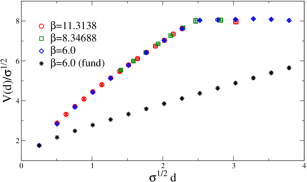
Finally, in Fig. 7 we show the continuum scaling of $V^{\mathrm{adj}}$ for three different values of the lattice spacing (which goes from $a\approx 0.11\,\mathrm{fm}$ at $\beta=6.0$ to $a\approx 0.057\,\mathrm{fm}$ at $\beta=11.3138$), with the static potential between fundamental charges being also shown for comparison. Additive constants have been fixed by imposing $V^{\mathrm{adj}}(2/\sqrt{\sigma})=7\sqrt{\sigma}$, and an almost perfect scaling is observed, which implies also in this case the absence of significant cut-off effects.

Figure 7: Continuum scaling of the adjoint static potential: data have been obtained on lattices with $L=32$ ($\beta=6.0$), $L=48$ ($\beta=8.34688$) and $L=64$ ($\beta=11.3138$). The potential between two fundamental charges for $\beta=6.0$ is also reported for comparison.

IV Conclusions

In this paper we have studied color flux tubes in a theory which displays string breaking, and in particular their behavior when the separation between the static sources approaches the string breaking distance $R_{c}$. For this purpose we used as testbed the three-dimensional SU(2) Yang-Mills theory with charges transforming in the adjoint representation of the gauge group.

We have shown that the adjoint flux tube, like the fundamental one, consists mainly of the longitudinal chromoelectric field for distances $d$ between the sources that are smaller than $R_{c}$. As the critical distance $R_{c}$ is approached, the longitudinal chromoelectric field gets strongly suppressed, becoming of the same size of the transverse fields at $R_{c}$. The disappearance of the flux tube is quite abrupt, and the value of $R_{10}(d,x_{t}=0)$ (which is related to square of longitudinal chromoelectric field inside the flux tube) decreases approximately by a factor of $3$ when the relative difference between $d$ and $R_{c}$ reduces below $10\%$.

This rapid disappearance is the one that could have been naively guessed from the behavior of the adjoint static potential $V^{\mathrm{adj}}(d)$, which suddenly switches from an approximately linear grow to a constant plateau at $d\simeq R_{c}$. We have however seen that precursors of string breaking are present for $d$ smaller than $R_{c}$, which are basically related to the failure of standard effective string theory. The scaling of the square width $w^{2}(d)$ of the flux tube with the distance $d$ follows (at least within the present accuracy) the expected logarithmic behaviour, but the value of the coefficient differs from the universal effective string prediction. Similarly, an analogous of the Luscher term is present also in $V^{\mathrm{adj}}(d)$, but again numerical data are not compatible with the expected universal coefficient.

Future studies should be aimed at extending this analysis to other models, to understand to which amount the phenomenology at string breaking observed in the three-dimensional SU(2) Yang-Mills case is generic and, in particular, is relevant for QCD. For the same reason it would be very interesting to investigate if there is a relation between the values of the coefficients $k_{w}$ and $k$ in Eqs. (12),(15) (or better, their deviations from the EST predictions) and some nonuniversal property of the theory, like its spectrum.

Acknowledgements Numerical simulations have been performed on the CSN4 cluster of the Scientific Computing Center at INFN-PISA. It is a pleasure to thank Michele Caselle for useful comments and discussions.

References

- [1] https://www.claymath.org/millennium-problems
- [2] M. Fukugita and T. Niuya, Phys. Lett. 132B, 374 (1983).
- [3] A. Di Giacomo, M. Maggiore and S. Olejnik, Phys. Lett. B 236, 199 (1990).
- [4] A. Di Giacomo, M. Maggiore and S. Olejnik, Nucl. Phys. B 347, 441 (1990).
- [5] G. S. Bali, K. Schilling and C. Schlichter, Phys. Rev. D 51, 5165 (1995) [hep-lat/9409005].
- [6] R. W. Haymaker, V. Singh, Y. C. Peng and J. Wosiek, Phys. Rev. D 53, 389 (1996) [hep-lat/9406021].
- [7] P. Cea and L. Cosmai, Phys. Rev. D 52, 5152 (1995) [hep-lat/9504008].
- [8] A. Allais and M. Caselle, JHEP 0901, 073 (2009) [arXiv:0812.0284 [hep-lat]].
- [9] F. Gliozzi, M. Pepe and U.-J. Wiese, Phys. Rev. Lett. 104, 232001 (2010) [arXiv:1002.4888 [hep-lat]].
- [10] F. Gliozzi, M. Pepe and U.-J. Wiese, JHEP 1101, 057 (2011) [arXiv:1010.1373 [hep-lat]].
- [11] N. Cardoso, M. Cardoso and P. Bicudo, Phys. Rev. D 88, 054504 (2013) [arXiv:1302.3633 [hep-lat]].
- [12] A. Amado, N. Cardoso and P. Bicudo, arXiv:1309.3859 [hep-lat].
- [13] M. Caselle, M. Panero and D. Vadacchino, JHEP 1602, 180 (2016) [arXiv:1601.07455 [hep-lat]].
- [14] M. S. Cardaci, P. Cea, L. Cosmai, R. Falcone and A. Papa, Phys. Rev. D 83, 014502 (2011) [arXiv:1011.5803 [hep-lat]].
- [15] P. Cea, L. Cosmai and A. Papa, Phys. Rev. D 86, 054501 (2012) [arXiv:1208.1362 [hep-lat]].
- [16] P. Cea, L. Cosmai, F. Cuteri and A. Papa, Phys. Rev. D 89, 094505 (2014) [arXiv:1404.1172 [hep-lat]].
- [17] P. Cea, L. Cosmai, F. Cuteri and A. Papa, JHEP 1606, 033 (2016) [arXiv:1511.01783 [hep-lat]].
- [18] M. Baker, P. Cea, V. Chelnokov, L. Cosmai, F. Cuteri and A. Papa, Eur. Phys. J. C 79, 478 (2019) [arXiv:1810.07133 [hep-lat]].
- [19] N. Battelli and C. Bonati, Phys. Rev. D 99, 114501 (2019) [arXiv:1903.10463 [hep-lat]].
- [20] F. Okiharu and R. M. Woloshyn, Nucl. Phys. Proc. Suppl. 129, 745 (2004) [hep-lat/0310007].
- [21] F. Bissey, F. G. Cao, A. R. Kitson, A. I. Signal, D. B. Leinweber, B. G. Lasscock and A. G. Williams, Phys. Rev. D 76, 114512 (2007) [hep-lat/0606016].
- [22] P. Bicudo, N. Cardoso and M. Cardoso, Prog. Part. Nucl. Phys. 67, 440 (2012) [arXiv:1111.0334 [hep-lat]].
- [23] A. S. Bakry, X. Chen and P. M. Zhang, Phys. Rev. D 91, 114506 (2015) [arXiv:1412.3568 [hep-lat]].
- [24] B. H. Wellegehausen, A. Wipf and C. Wozar, Phys. Rev. D 83, 016001 (2011) [arXiv:1006.2305 [hep-lat]].
- [25] P. Cea, L. Cosmai, F. Cuteri and A. Papa, Phys. Rev. D 95, 114511 (2017) [arXiv:1702.06437 [hep-lat]].
- [26] C. Bonati, S. Calì, M. D’Elia, M. Mesiti, F. Negro, A. Rucci and F. Sanfilippo, Phys. Rev. D 98, 054501 (2018) [arXiv:1807.01673 [hep-lat]].
- [27] O. Philipsen and H. Wittig, Phys. Rev. Lett. 81, 4056 (1998) Erratum: [Phys. Rev. Lett. 83, 2684 (1999)] [hep-lat/9807020].
- [28] C. E. Detar, O. Kaczmarek, F. Karsch and E. Laermann, Phys. Rev. D 59, 031501 (1998) [arXiv:hep-lat/9808028 [hep-lat]].
- [29] C. W. Bernard, T. A. DeGrand, C. E. Detar, P. Lacock, S. A. Gottlieb, U. M. Heller, J. Hetrick, K. Orginos, D. Toussaint and R. L. Sugar, Phys. Rev. D 64, 074509 (2001) [arXiv:hep-lat/0103012 [hep-lat]].
- [30] F. Gliozzi and A. Rago, Nucl. Phys. B 714, 91 (2005) [hep-lat/0411004].
- [31] G. S. Bali et al. [SESAM Collaboration], Phys. Rev. D 71, 114513 (2005) [hep-lat/0505012].
- [32] J. Bulava, B. Hörz, F. Knechtli, V. Koch, G. Moir, C. Morningstar and M. Peardon, Phys. Lett. B 793, 493 (2019) [arXiv:1902.04006 [hep-lat]].
- [33] P. W. Stephenson, Nucl. Phys. B 550, 427 (1999) [hep-lat/9902002].
- [34] O. Philipsen and H. Wittig, Phys. Lett. B 451, 146 (1999) [hep-lat/9902003].
- [35] S. Kratochvila and P. de Forcrand, Nucl. Phys. B 671, 103 (2003) [hep-lat/0306011].
- [36] M. Pepe and U.-J. Wiese, Phys. Rev. Lett. 102, 191601 (2009) [arXiv:0901.2510 [hep-lat]].
- [37] K. Kallio and H. D. Trottier, Phys. Rev. D 66, 034503 (2002) [arXiv:hep-lat/0001020 [hep-lat]].
- [38] A. Agarwal, D. Karabali and V. P. Nair, Nucl. Phys. B 790, 216 (2008) [arXiv:0705.0394 [hep-th]].
- [39] K. G. Wilson, Phys. Rev. D 10, 2445 (1974).
- [40] M. Creutz, Phys. Rev. D 21, 2308 (1980).
- [41] A. D. Kennedy and B. J. Pendleton, Phys. Lett. 156B, 393 (1985).
- [42] M. Creutz, Phys. Rev. D 36, 515 (1987).
- [43] M. J. Teper, Phys. Rev. D 59, 014512 (1998) [hep-lat/9804008].
- [44] G. Parisi, R. Petronzio and F. Rapuano, Phys. Lett. 128B, 418 (1983).
- [45] M. Luscher and P. Weisz, JHEP 0109, 010 (2001) [hep-lat/0108014].
- [46] M. Luscher, Nucl. Phys. B 180, 317 (1981).
- [47] B. B. Brandt and M. Meineri, Int. J. Mod. Phys. A 31, 1643001 (2016) [arXiv:1603.06969 [hep-th]].