Neutron-neutron scattering length from
$\pi^{+}$ photoproduction on the deuteron

Abstract

We discuss the possibility of extracting the neutron-neutron scattering length $a_{nn}$ and effective range $r_{nn}$ from cross-section data ($d^{2}\sigma/dM_{nn}/d\Omega_{\pi}$), as a function of the $nn$ invariant mass $M_{nn}$, for $\pi^{+}$ photoproduction on the deuteron ($\gamma d\to\pi^{+}nn$). The analysis is based on a $\gamma d\to\pi^{+}nn$ reaction model in which realistic elementary amplitudes for $\gamma p\to\pi^{+}n$, $NN\to NN$, and $\pi N\to\pi N$ are incorporated. We demonstrate that the $M_{nn}$ dependence (line shape) of a ratio $R_{\rm th}$, $d^{2}\sigma/dM_{nn}/d\Omega_{\pi}$ normalized by $d\sigma/d\Omega_{\pi}$ for $\gamma p\to\pi^{+}n$ and the nucleon momentum distribution inside the deuteron, at the kinematics with $\theta_{\pi}=0^{\circ}$ and $E_{\gamma}\sim 250$ MeV is particularly useful for extracting $a_{nn}$ and $r_{nn}$ from the corresponding $R_{\rm exp}$ data. We found that $R_{\rm exp}$ with 2% error, resolved into an $M_{nn}$ bin width of 0.04 MeV (corresponding to a $p_{\pi}$ bin width of 0.05 MeV$/c$), can determine the $a_{nn}$ and $r_{nn}$ with uncertainties of $\pm 0.21$ and $\pm 0.06$ fm, respectively, if $a_{nn}=-18.9$ fm and $r_{nn}=2.75$ fm. The requirement of such narrow bin widths indicates that the momenta of the incident photon and emitted $\pi^{+}$ must be measured at high resolutions. This can be achieved by utilizing virtual photons of very low $Q^{2}$ from electron scattering at the Mainz Microtron facility. The method proposed herein for determining the $a_{nn}$ and $r_{nn}$ from $\gamma d\to\pi^{+}nn$ has a great experimental advantage over the previous method of utilizing $\pi^{-}d\to\gamma nn$ for not requiring the formidable task of controlling the neutron detection efficiency and its uncertainty.

I Introduction

Charge symmetry (CS) is an important concept used to describe many facets of nuclear physics cs_review; miller2. It leads to a consequence that observables hardly change when all protons and neutrons in a nuclear system are replaced by neutrons and protons, respectively. For example, the excited states of mirror nuclei have identical energy levels and spin-parity assignments. The CS can be more generally defined by the invariance under the rotation by $180^{\circ}$ about the $y$-axis in the isospin space. This rotation corresponds to the interchange of $u$ and $d$ quarks at the quark level and the interchange of protons and neutrons at the hadron level.

Within the Standard Model, the CS is broken due to the differences among $u$ and $d$ quark masses and electromagnetic (EM) effects. These elementary effects appear in hadron phenomenology in various ways, e.g., the neutron ($n$) and proton ($p$) mass difference of 1.3 MeV and the small charge-dependent component of nuclear force that breaks the CS at the order of a few percentages. In terms of the hadronic degrees of freedom, the CS breaking (CSB) of nuclear force can be described by a mixing of the neutral rho meson ($\rho^{0}$) and omega meson ($\omega$) in one boson exchange mechanism miller2 and the $n$-$p$ mass difference. This CSB force could explain the following experimental observations: the 0.7-MeV difference in the binding energies between ³H and ³He (mirror nuclei); the difference in the analyzing powers $A_{n}(\theta_{n})\neq A_{p}(\theta_{p})$ at the same angle $\theta_{n}=\theta_{p}$ for $np$ scattering abegg; the forward-backward asymmetry $d\sigma/d\Omega_{\pi}(\theta)\neq d\sigma/d\Omega_{\pi}(\pi-\theta)$ in the deuteron ($d$) formation reaction emitting a neutral pion ($np\to d\pi^{0}$) csb_np_dpi0. A large difference in the excitation energies between the $A=4$ mirror hypernuclei, i.e., ${}^{4}_{\Lambda}$H and ${}^{4}_{\Lambda}$He, has been recently reported csb_hyper_jparc; csb_hyper_a1. It is possible that CSB occurs more strongly in hypernuclei than in ordinary nuclei. A complete understanding of CSB still remains an open issue in nuclear physics. To reveal the cause of the CSB observed in few-baryon systems, it is of critical importance to experimentally investigate the differences between low-energy elementary $nn$ and $pp$ scatterings as well as between $\Lambda n$ and $\Lambda p$ scatterings.

Low-energy $NN$ scattering is characterized by the scattering length $a$ and effective range $r$ through an effective-range expansion of the $S$-wave phase shift $\delta(p)$ as follows:

$$p\cot\delta(p)=-\frac{1}{a}+\frac{1}{2}\,r\,p^{2}+O(p^{4}),$$ (1)

where $p$ denotes the momentum of the nucleon ($N$) in the $NN$ center-of-mass (CM) frame. Note that a positive or negative $a$ value indicates a repulsion or attraction, respectively, in this definition. The experimentally obtained $a$ and $r$ parameters of the spin-singlet (${}^{1}\!S_{0}$) states are:

$$\left\{\begin{array}[]{lll}a_{nn}=-18.9\pm 0.4{\rm\ fm},&r_{nn}=2.75\pm 0.11{\rm\ fm}&{\rm for\ }nn,\\ a_{np}=-23.74\pm 0.02{\rm\ fm},&r_{np}=2.77\pm 0.05{\rm\ fm}&{\rm for\ }np,{\rm\ and}\\ a_{pp}=-17.3\pm 0.4{\rm\ fm},&r_{pp}=2.85\pm 0.04{\rm\ fm}&{\rm for\ }pp,\\ \end{array}\right.$$ (2)

where the EM effects have already been corrected. The scattering length $a_{np}$ in the $np$ system is significantly different from the other two, i.e., $a_{nn}$ and $a_{pp}$, suggesting charge independence breaking. The CSB is significant at the 1.6-fm difference between $a_{nn}$ and $a_{pp}$. Moreover, while the error of $a_{nn}$ predominantly stems from the statistical uncertainty in the experiments, that of $a_{pp}$ originates from the systematic uncertainty of removing the EM effects.

Thus far, several different $a_{nn}$ values ranging from $-19$ to $-16$ fm have been reported (see Ref. gardestig_review for a recent review), but no consensus has been reached on which value is correct. One experimental difficulty is that conducting an $nn$ scattering experiment, through which the $a_{nn}$ value can be determined directly, is nearly impossible because a realistic free neutron target does not exist. Therefore, the primary experimental results for $a_{nn}$ are from two different types of experiments utilizing the final-state $nn$ interaction (indirect determination): (i) the three-body breakup reaction of $nd\to nnp$; (ii) the radiative capture of a stopped negative pion on the deuteron ($\pi^{-}d\to nn\gamma$).

For type (i) experiments, excluding those before 1973, $a_{nn}$ values are extracted from the data with the exact solution of the Faddeev equation for $nd\to nnp$ faddeev. Significantly different $a_{nn}$ values have been obtained from the same reaction:

$$\left\{\begin{array}[]{l@{}l@{}l}a_{nn}=-16.1\pm 0.4{\rm\ fm\ }&(E_{n}=25.3{\rm\ MeV},&{\ }np{\rm\ detected}~\text{\cite[cite]{\@@bibref{Authors Phrase1YearPhrase2}{huhn}{\@@citephrase{(}}{\@@citephrase{)}}}}),\\ a_{nn}=-18.7\pm 0.7{\rm\ fm\ }&(E_{n}=13.0{\rm\ MeV},&{\ }nnp{\rm\ detected}~\text{\cite[cite]{\@@bibref{Authors Phrase1YearPhrase2}{gonz}{\@@citephrase{(}}{\@@citephrase{)}}}}),{\rm\ and}\\ a_{nn}=-16.5\pm 0.9{\rm\ fm\ }&(E_{n}=17.4{\rm\ MeV},&{\ }p{\rm\ detected}~\text{\cite[cite]{\@@bibref{Authors Phrase1YearPhrase2}{wits}{\@@citephrase{(}}{\@@citephrase{)}}}}).\\ \end{array}\right.$$ (3)

The primary concern with these results is the possibility of large three-body force effects. As the details of these effects are not yet well-established, the systematic uncertainty associated with them could be underestimated.

The type (ii) experiments of $\pi^{-}d\to nn\gamma$ are considered as a more reliable method to determine the $a_{nn}$ value because only $nn$ scattering without three-body force effects occurs in the final state. The obtained experimental value is $a_{nn}=-18.9\pm 0.4$ fm after including the correction of $\Delta a_{nn}\sim-0.3$ fm from the magnetic-moment interaction between $nn$ chen. The difficulty of experimentally studying $\pi^{-}d\to nn\gamma$ lies in detecting low-energy neutrons. The efficiency of detecting the neutrons depends on their kinetic energies and is sensitive to the detector threshold measured in the electron-equivalent energy. In Refs. chen; howell, the detector efficiencies were checked at neutron kinetic energies from 5 to 13 MeV using energy-tagged neutrons produced in the ${}^{2}{\rm H}(d,n){}^{3}{\rm He}$ reaction. However, a direct measurement has not yet been performed for detector efficiencies around $\sim$2.4 MeV, at which neutrons affected by the final-state interaction are expected to appear from $\pi^{-}d\to nn\gamma$. Regarding theory, a series of works have been conducted based on phenomenological GGS and dispersion-relation approaches Teramond. A more recent work has also been done based on the chiral effective field theory anders. Due to the dominance of the Kroll-Ruderman term, the pion photoproduction amplitude is rather well-controlled. It has been reported that the primary theoretical uncertainty stems from the off-shell behavior of the $nn$ rescattering amplitude.

Another possible method of determining the $a_{nn}$ value is to utilize the final-state $nn$ interaction in the $\gamma d\to\pi^{+}nn$ reaction. This possibility was pointed out by Lensky et al. prev, who studied the reaction with the chiral perturbation theory. However, their calculation is limited to the energy region close to the pion-production threshold (photon energy up to 20 MeV above the threshold, corresponding to an emitted pion momentum less than 80 MeV$/c$). It is difficult to experimentally detect such a low-momentum $\pi^{+}$ before its decay. Alternatively, let us consider the reaction at an incident photon energy of $E_{\gamma}=200$–300 MeV. This energy region is between the pion production threshold ($E_{\gamma}\sim 150$ MeV) and the excitation energy of the delta baryon ($\Delta(1232)\,P_{33}$) ($E_{\gamma}\sim 340$ MeV), assuming that the quasi-free $\gamma p\to\pi^{+}n$ reaction occurs on the initial nucleon at rest inside the deuteron. Here, we choose to detect the $\pi^{+}$s emitted at $\theta_{\pi}\simeq 0^{\circ}$ from the photon direction, and only those near the maximum momentum are of interest. In this particular kinematics, the relative momentum of $nn$ is low, and $nn$ are expected to strongly interact with each other. Additionally, this would efficiently prevent a pion created in $\gamma N\to\pi N$ from rescattering on the spectator nucleon because the $\pi N$ interaction is weak at low energies and/or the spectator nucleon is required to have a large momentum, which is largely suppressed in the deuteron. This seems to be an ideal condition with which to study low-energy neutron-neutron scattering, thereby determining the $a_{nn}$ as well as $r_{nn}$ values.

For extracting $a_{nn}$ from $\pi^{-}d\to\gamma nn$ or $\gamma d\to\pi^{+}nn$, the experimental challenge is to obtain the $nn$ invariant mass ($M_{nn}$) distribution at $M_{nn}\sim 2m_{n}$ with high statistics and high resolution. In this respect, we find that $\gamma d\to\pi^{+}nn$ is more advantageous than $\pi^{-}d\to\gamma nn$ because we can avoid neutron detection, the efficiency of which could significantly increase the systematic uncertainty. We only need to detect $\pi^{+}$s with momenta of 120–250 MeV/$c$ once the incident photon energies have been determined to a sufficient precision. Thus, it seems valuable to analyze $\gamma d\to\pi^{+}nn$ data and extract the $a_{nn}$ value, which is both independent of and alternative to those from previous methods using $\pi^{-}d\to\gamma nn$ and $nd$ scattering data. To extract the $a_{nn}$ and $r_{nn}$ from the $\gamma d\to\pi^{+}nn$ data in a controlled manner, we must estimate possible theoretical uncertainties. Therefore, in this work, we use a theoretical model for the $\gamma d\to\pi^{+}nn$ reaction and examine the reaction at the particular kinematical conditions of $E_{\gamma}=200$–300 MeV, $\theta_{\pi}\sim 0^{\circ}$, and $M_{nn}\sim 2m_{n}$. Through a theoretical analysis of $\gamma d\to\pi^{+}nn$, we find that the kinematics and shape of the $M_{nn}$ distribution are indeed suitable for studying low-energy $nn$ scattering. We also assess possible theoretical uncertainties of the $M_{nn}$ distribution needed when extracting the $a_{nn}$ and $r_{nn}$ values from the corresponding data. Finally, we conduct a Monte Carlo simulation to extract the $a_{nn}$ and $r_{nn}$ from the data, prepared with different precisions and $M_{nn}$ bin widths, and estimate their uncertainties. This analysis leads to the proposal of an alternative and more reliable method of extracting the $a_{nn}$ and $r_{nn}$.

The rest of this paper is organized as follows: In Sec. II, we discuss the theoretical formalism used to study $\gamma d\to\pi^{+}nn$. The numerical results are presented and discussed in Sec. III. Sec. IV is devoted to a discussion on the experimental strategy of measuring $\gamma d\to\pi^{+}nn$ with high resolution using virtual photons of a low $Q^{2}$ ($<0.01$ GeV²). Finally, a summary follows in Sec. V.

II Formalism

II.1 The $\gamma d\to\pi^{+}nn$ reaction model based on the dynamical coupled-channels model

Our starting point to develop a $\gamma d\to\pi^{+}nn$ reaction model is the elementary amplitudes for the $\gamma N\to\pi N$ and $\pi N\to\pi N$ processes. Here, we employ the elementary amplitudes generated by a dynamical coupled-channels (DCC) model knls13; knls16. The DCC model includes meson-baryon channels relevant to the nucleon resonance and $\Delta$ resonance (generically referred to as $N^{*}$) region, such as $\pi N,\eta N,K\Lambda,K\Sigma$, and also $\pi\Delta,\sigma N,\rho N$ which couple to $\pi\pi N$. The $\gamma^{(*)}N$ channel is also considered perturbatively. The meson-baryon interaction potentials comprise meson-exchange non-resonant and (bare) $N^{*}$-excitation resonant mechanisms. The gauge invariance is satisfied at the tree level. Upon solving the coupled-channel Lippmann-Schwinger equation, with off-shell effects fully considered, the unitary DCC amplitudes are obtained. The DCC model was developed through a comprehensive analysis of the $\pi N,\gamma N\to\pi N,\eta N,K\Lambda$, and $K\Sigma$ data in the CM energy ($W$) region from the channel thresholds to $W\ \raise 1.29167pt\hbox{$<$\kern-7.5pt\lower 4.30554pt\hbox{$\sim$}}\ 2.1$ GeV. The model provides a reasonable description of the data included in the fits, and the properties of all the well-established nucleon resonances have been extracted from the obtained amplitudes. The DCC model was extended to a finite $Q^{2}$ region via analyzing electron-induced data dcc_nu as well as to neutrino-induced reactions via developing the axial current amplitudes dcc_nu; nu-review; nu-comp.

Figure 1: Differential cross sections of $\gamma p\to\pi^{+}n$ from the DCC model. The CM energy $W$ is indicated in each panel. The $W=1121$, 1162, and 1201 MeV energies correspond to the incident photon energies of $E_{\gamma}\simeq 200$, 250, and 300 MeV, respectively. The data are taken from Ref. gp-data. The errors shown are statistical only.

The $\gamma p\to\pi^{+}n$ elementary amplitude is of primary importance when developing a $\gamma d\to\pi^{+}nn$ model. Therefore, it is reassuring to see in Fig. 1 that the DCC model well describes the $\gamma p\to\pi^{+}n$ cross-section data in the energy region relevant to this work. However, data are unavailable for the forward direction ($\cos\theta_{\pi}^{\rm\,CM}=1$), which is particularly important for our purpose. Moreover, the data shown in Fig. 1 have additional systematic errors. These facts could raise concern as to whether we can develop a $\gamma d\to\pi^{+}nn$ model that reaches the precision required to extract the $a_{nn}$ from data. As will be discussed later, when extracting the $a_{nn}$, we use a method that largely cancels out the normalization uncertainty of the elementary $\gamma p\to\pi^{+}n$ amplitudes.

With the DCC model as the starting point, it is straightforward to extend the model to a $\pi NN$ system following the well-established multiple scattering theory kmt. In this work, we consider the impulse and first-order rescattering terms, as depicted in Fig. 2, wherein higher order rescattering terms are truncated. This setup, including up to the first-order rescattering, has been used in previous works arenhover; fix; lev06; sch10; wsl15; tara-1; dcc-deu4 and shown to provide a reasonable description of $\gamma d\to\pi NN$ data with significant rescattering effects. As we will see, this truncation is a good approximation for the particular kinematics considered in this work.

Similar DCC-based deuteron reaction models have been successfully applied to solve several problems of current interest. We proposed a novel method to determine the $\eta N$ scattering length using $\gamma d\to\eta pn$ data at a special kinematics in Ref. dcc-deu1. In Ref. dcc-deu2, the extraction of neutron-target observables from $\gamma d\to\pi NN$ data was examined, and some rescattering effects observed in the data were elucidated for the first time. In Ref. dcc-deu3, neutrino-nucleon cross sections from neutrino-deuteron data were corrected by estimating the rescattering effects, significantly contributing to neutrino oscillation experiments nustec.

II.2 Cross-section formula

Figure 2: The diagrams for $\gamma d\to\pi^{+}nn$ considered in this work; (a) impulse, (b) $NN$ rescattering, and (c) $\pi N$ rescattering mechanisms. We introduced $\bm{Q}\equiv\bm{q}-\bm{k}$ and $\bm{x}\equiv\bm{q}-\bm{p}_{2}+\bm{l}$. The shaded ellipses are elementary amplitudes from the DCC model.

The unpolarized differential cross-section formula for $\gamma(\bm{q})+d(\bm{p}_{d})\to\pi^{+}(\bm{k})+n_{1}(\bm{p}_{1})+n_{2}(\bm{p}_{2})$ in the laboratory frame ($\bm{p}_{d}=0$) is given as:

$$\frac{d^{2}\sigma(E_{\gamma})}{d\Omega_{\bm{k}}dM_{nn}}={1\over 12}\sum_{\lambda,s_{d}}\sum_{s_{1},s_{2}}\frac{(2\pi)^{4}}{4E_{\gamma}}\frac{1}{2E_{d}(\bm{p}_{d})}\int d\Omega_{\bm{p}_{nn}}{p_{nn}k^{2}m_{n}^{2}\over|kE-\bm{q}\!\cdot\!\hat{k}\,E_{\pi}(\bm{k})|}\;|M(E)|^{2}\ ,$$ (4)

where $\lambda$ is the photon polarization and $s_{d}$ ($s_{i}$) is the $z$-component of the deuteron (neutron $i$) spin, with a factor of $1/12$ for averaging the initial spins ($1/2\times 1/3$) and for the identity of the final two neutrons ($1/2$). The energy $E_{x}$ for particle $x$ depends on the particle mass ($m_{x}$) and momentum ($\bm{p}_{x}$) as $E_{x}=\sqrt{\bm{p}^{2}_{x}+m^{2}_{x}}$, and the total energy in the laboratory frame is $E=m_{d}+E_{\gamma}$. The $\bm{p}_{nn}$ denotes the momentum of a neutron in the $n_{1}n_{2}$ CM frame. We simply wrote the magnitudes of the momenta as $k\equiv|\bm{k}|$ and $\hat{k}\equiv\bm{k}/|\bm{k}|$. The quantity $M(E)$ is the Lorentz-invariant amplitude defined below.

As discussed in subsection II.1, we describe the $\gamma d\to\pi^{+}nn$ reaction by considering the impulse [$t_{{\rm imp}}$, Fig. 2(a)], $NN$ rescattering [$t_{NN}$, Fig. 2(b)], and $\pi N$ rescattering [$t_{\pi N}$, Fig. 2(c)] mechanisms. The corresponding amplitudes are written using the kinematical variables defined in Fig. 2 as follows (see Ref. dcc-deu4 for a more detailed discussion):

$$t_{{\rm imp}} = \sqrt{2}\sum_{s_{1}^{\prime},t^{\prime}_{1}}\langle{\pi(\bm{k},t_{\pi})\,N_{1}(\bm{p}_{1},s_{1},t_{1})}|t_{\pi N,\gamma N}(M_{\pi N_{1}})|{\gamma(\bm{q},\lambda)\,N_{1}^{\prime}(-\bm{p}_{2},s_{1}^{\prime},t^{\prime}_{1})}\rangle$$ (5)

$$\times\langle{N_{1}^{\prime}(-\bm{p}_{2},s_{1}^{\prime},t^{\prime}_{1})\,N_{2}(\bm{p}_{2},s_{2},t_{2})}|{\Psi_{d}(s_{d})}\rangle\ ,$$

$$t_{NN} = \sqrt{2}\sum_{s_{1}^{\prime},\tilde{s}_{1}^{\prime},s_{2}^{\prime},t^{\prime}_{1}}\int d\bm{l}\$$ (6)

$$\times\langle{N_{1}(\bm{p}_{1},s_{1},t_{1})\,N_{2}(\bm{p}_{2},s_{2},t_{2})}|t_{NN,NN}(M_{N_{1}N_{2}})|{\tilde{N}^{\prime}_{1}(\bm{q}-\bm{k}+\bm{l},\tilde{s}^{\prime}_{1},t_{1})\,N^{\prime}_{2}(-\bm{l},s^{\prime}_{2},t_{2})}\rangle$$

$$\times{\langle{\pi(\bm{k},t_{\pi})\,\tilde{N}_{1}^{\prime}(\bm{q}-\bm{k}+\bm{l},\tilde{s}_{1}^{\prime},t_{1})}|t_{\pi N,\gamma N}(W)|{\gamma(\bm{q},\lambda)\,N_{1}^{\prime}(\bm{l},s_{1}^{\prime},t^{\prime}_{1})}\rangle\over E-E_{N}(\bm{q}-\bm{k}+\bm{l})-E_{N}(-\bm{l})-E_{\pi}(\bm{k})+i\epsilon}$$

$$\times\langle{N_{1}^{\prime}(\bm{l},s_{1}^{\prime},t^{\prime}_{1})\,N_{2}^{\prime}(-\bm{l},s_{2}^{\prime},t_{2})}|{\Psi_{d}(s_{d})}\rangle\ ,{\rm and}$$

$$t_{\pi N} = \sqrt{2}\sum_{s_{1}^{\prime},s_{2}^{\prime}}\sum_{t_{1}^{\prime},t_{2}^{\prime},t^{\prime}_{\pi}}\int d\bm{l}\langle{\pi(\bm{k},t_{\pi})\,N_{1}(\bm{p}_{1},s_{1},t_{1})}|t_{\pi N,\pi N}(M_{\pi N_{1}})|{\pi(\bm{q}-\bm{p}_{2}+\bm{l},t^{\prime}_{\pi})\,N_{1}^{\prime}(-\bm{l},s^{\prime}_{1},t_{1}^{\prime})}\rangle$$ (7)

$$\times{\langle{\pi(\bm{q}-\bm{p}_{2}+\bm{l},t^{\prime}_{\pi})\,N_{2}(\bm{p}_{2},s_{2},t_{2})}|t_{\pi N,\gamma N}(W)|{\gamma(\bm{q},\lambda)\,N_{2}^{\prime}(\bm{l},s_{2}^{\prime},t_{2}^{\prime})}\rangle\over E-E_{N}(\bm{p}_{2})-E_{N}(-\bm{l})-E_{\pi}(\bm{q}-\bm{p}_{2}+\bm{l})+i\epsilon}$$

$$\times\langle{N_{1}^{\prime}(-\bm{l},s_{1}^{\prime},t_{1}^{\prime})\,N_{2}^{\prime}(\bm{l},s_{2}^{\prime},t_{2}^{\prime})}|{\Psi_{d}(s_{d})}\rangle\ .$$

The exchange terms are obtained from Eqs. (5)–(7) by flipping the overall sign and interchanging all subscripts 1 and 2 for nucleons in the intermediate and final $\pi NN$ states. In the above expressions, the deuteron state with spin projection $s_{d}$ is denoted as $|{\Psi_{d}(s_{d})}\rangle$; $|{N(\bm{p},s,t)}\rangle$ is the nucleon state with momentum $\bm{p}$ and spin and isospin projections $s$ and $t$, respectively; $|{\gamma(\bm{q},\lambda)}\rangle$ is the photon state with momentum $\bm{q}$ and polarization $\lambda$; $|{\pi(\bm{k},t_{\pi})}\rangle$ is the pion state with momentum $\bm{k}$ and isospin projection $t_{\pi}$. The two-body elementary amplitudes depend on the $\pi N_{1}$ and $N_{1}N_{2}$ invariant masses given by

$$M_{\pi N_{1}} = \sqrt{[E_{\pi}(\bm{k})+E_{N}(\bm{p}_{1})]^{2}-(\bm{k}+\bm{p}_{1})^{2}}\ ,{\rm and}$$ (8)

$$M_{N_{1}N_{2}} = \sqrt{[E_{N}(\bm{p}_{1})+E_{N}(\bm{p}_{2})]^{2}-(\bm{p}_{1}+\bm{p}_{2})^{2}}\ ,$$ (9)

respectively, and also the $\gamma N$ invariant mass calculated according to the spectator approximation:

$$W = \sqrt{[E-E_{N}(-\bm{l})]^{2}-(\bm{l}+\bm{q})^{2}}\ .$$ (10)

The two-nucleon energy in the propagator of the $NN$ rescattering amplitude in Eq. (6) is calculated via a non-relativistic approximation:

$$E_{N}(\bm{q}-\bm{k}+\bm{l})+E_{N}(-\bm{l})\simeq\sqrt{(2m_{N})^{2}+(\bm{q}-\bm{k})^{2}}+{(\bm{q}/2-\bm{k}/2+\bm{l})^{2}\over m_{N}}\ .$$ (11)

Finally, the Lorentz-invariant scattering amplitude [$M(E)$] used in Eq. (4) is expressed with the amplitudes of Eqs. (5)–(7) by:

$$M(E) = \sqrt{{8E_{\gamma}E_{d}(\bm{p}_{d})E_{\pi}(\bm{k})E_{n}(\bm{p}_{1})E_{n}(\bm{p}_{2})}\over m_{n}^{2}}$$ (12)

$$\times\Big(t_{{\rm imp}}(E)+t_{NN}(E)+t_{\pi N}(E)+\{{\rm exchange\ terms}\}\Big)\ .$$

Regarding the off-shell elementary amplitudes used in Eqs. (5)–(7), we use those generated by the DCC model for the pion photoproduction amplitudes ($t_{\pi N,\gamma N}$) and pion-nucleon scattering amplitudes ($t_{\pi N,\pi N}$). Moreover, we generate the half off-shell $NN$ scattering amplitudes ($t_{NN,NN}$) and the deuteron wave function ($\Psi_{d}$) using high-precision phenomenological $NN$ potentials.

III Results and discussion

Figure 3: (Left) The $nn$ invariant mass ($M_{nn}$) distribution for $\gamma d\to\pi^{+}nn$. The incident photon energy is $E_{\gamma}=250$ MeV, and the pion emission angle is fixed at $\theta_{\pi}=0^{\circ}$. The blue dashed, black dotted, and red solid curves are calculated with the impulse, impulse + $NN$ rescattering, and impulse + $NN+\pi N$ rescattering mechanisms, respectively. The emitted pion momentum is indicated on the upper horizontal axis. The inset shows the small $M_{nn}$ region. (Right) Ratio $R_{\rm th}$ defined in Eq. (13) for the same condition as the left panel.

In Fig. 3(left), we show the neutron-neutron invariant mass ($M_{nn}$) distribution ($d^{2}\sigma/dM_{nn}/d\Omega_{\pi}$ as a function of $M_{nn}$) for $\gamma d\to\pi^{+}nn$ at $E_{\gamma}=250$ MeV. Here, we use the CD-Bonn potential cdbonn to describe the $NN$ rescattering and the deuteron wave function. The pion emission angle is fixed at $\theta_{\pi}=0^{\circ}$. We focus on a small $M_{nn}$ region, as we are interested in the neutron-neutron scattering there. The impulse contribution has a quasi-free peak at $M_{nn}-2m_{n}\sim 1.3$ MeV. In this particular kinematics, the $NN$ rescattering contribution is large and creates a sharp peak at $M_{nn}\sim 2m_{n}$. This is due to the strong $NN$ interaction in the ${}^{1}\!S_{0}$ wave at low energies. On the other hand, the $\pi N$ rescattering contribution hardly changes the cross sections. This indicates that the pion is well separated from the $nn$ system in this kinematics; thus, the multiple scattering effect beyond the first-order rescattering is negligible. As such, this is a favorable kinematics for our model considering the diagrams in Fig. 2.

Next, we introduce a ratio $R_{\rm th}$, defined by:

$$R_{\rm th}=\left[\frac{d^{2}\sigma(E_{\gamma})}{d\Omega_{\bm{k}}dM_{nn}}\right]\bigg/\left[\frac{d^{2}\sigma_{\rm conv}(E_{\gamma})}{d\Omega_{\bm{k}}dM_{nn}}\right]\ ,$$ (13)

where the numerator is given in Eq. (4) including the impulse + $NN+\pi N$ rescattering mechanism. The denominator is defined by:

$$\frac{d^{2}\sigma_{\rm conv}(E_{\gamma})}{d\Omega_{\bm{k}}dM_{nn}}=\frac{d\sigma_{\gamma p\to\pi^{+}n}(E_{\gamma})}{d\Omega_{\bm{k}}}\int d^{3}p_{s}{m_{n}\over E_{n}(p_{s})}|\Psi_{d}(p_{s})|^{2}\delta(M_{nn}-{\cal M}_{nn}(\bm{p}_{s},E_{\gamma}))\ ,$$ (14)

with

$${\cal M}_{nn}(\bm{p}_{s},E_{\gamma})=\sqrt{(E_{n}(\bm{q}-\bm{k}-\bm{p}_{s})+E_{n}(\bm{p}_{s}))^{2}-(\bm{q}-\bm{k})^{2}}\ ,$$ (15)

and $d\sigma_{\gamma p\to\pi^{+}n}/d\Omega_{\bm{k}}$ is the differential cross section for $\gamma p\to\pi^{+}n$ in the laboratory frame. Eq. (14) could be derived from Eq. (4) via the following prescriptions: (i) consider only the impulse mechanism; (ii) use the $\gamma p\to\pi^{+}n$ amplitudes, assuming that the initial proton is at rest and free (without binding energy) inside the deuteron; (iii) ignore the interference with the exchange term; (iv) ignore the deuteron $D$-wave contribution. The deviation of $R_{\rm th}$ from one is a rough measure of the rescattering effects. The practical advantage of using $R_{\rm th}$ over the cross section itself is that the overall normalization uncertainty of the $\gamma p\to\pi^{+}n$ amplitudes is largely canceled. This uncertainty is primarily a carry-over from that in the $\gamma p\to\pi^{+}n$ data fitted. The ratio is also advantageous from an experimental viewpoint because the counterpart $R_{\rm exp}$ is given with measurable cross sections for proton and deuteron targets and the deuteron wave function; the systematic uncertainty in the overall normalization associated with the number of incident particles, the target thickness, and the solid angle for pion detection is also largely canceled in $R_{\rm exp}$. We present $R_{\rm th}$ in Fig. 3(right) at the same kinematical setting as the left panel. Once again, a strong rescattering effect can clearly be observed at $M_{nn}\sim 2m_{n}$.

Figure 4: Same as in Fig. 3 but for the incident photon energy of $E_{\gamma}=300$ MeV.

Figure 5: Same as in Fig. 3 but for the incident photon energy of $E_{\gamma}=200$ MeV.

Next, we examine the results at different $E_{\gamma}$ values. In Fig. 4, the $d^{2}\sigma/d\Omega_{\pi}/dM_{nn}$ and $R_{\rm th}$ are given for $E_{\gamma}=300$ MeV. While the line shapes are rather similar to those in Fig. 3, the pion rescattering effect is discernible at this energy. To reduce the theoretical uncertainty, it is best to avoid kinematics wherein the pion rescattering effect is non-negligible. The result for $E_{\gamma}=200$ MeV is shown in Fig. 5, which is qualitatively similar to Fig. 3. At low photon energies, a contribution from the elementary $\gamma p\to\pi^{+}n$ amplitude in the subthreshold region could be non-negligible. When the loop momentum becomes large, as in Figs. 2(b) and (c), the $W$ for the elementary $\gamma p\to\pi^{+}n$ amplitude, given by Eq. (10), falls below the $\pi N$ threshold. We found this contribution to be $\sim 2$% to the $\gamma d\to\pi^{+}nn$ cross sections. As data are absent for testing the subthreshold amplitude, it is best to use a higher $E_{\gamma}$ to suppress this contribution. We observed that the subthreshold contribution was negligible for $E_{\gamma}\ \raise 1.29167pt\hbox{$>$\kern-7.5pt\lower 4.30554pt\hbox{$\sim$}}\ 250$ MeV. Thus, we choose to study $\gamma d\to\pi^{+}nn$ at $E_{\gamma}=250$ MeV.

Figure 6: The $M_{nn}$ distributions for $\gamma d\to\pi^{+}nn$ at different pion-emission angles ($E_{\gamma}=250$ MeV). The red solid, black dotted, blue dashed, and magenta dash-dotted curves represent $\theta_{\pi}$=0^∘, 15^∘, 30^∘, and 45^∘, respectively.

We examine the pion emission angle dependence of the $\gamma d\to\pi^{+}nn$ cross section as well. The $M_{nn}$ distributions of different angles are shown in Fig. 6. The emission angle is changed from $0^{\circ}$ to $45^{\circ}$ in the laboratory frame. In the small $M_{nn}$ region, which is the most sensitive to the $nn$ scattering length, the cross section is significantly larger for smaller emission angles. Thus, from a statistical viewpoint, a small emission angle $\theta_{\pi}\sim 0^{\circ}$ is favorable to measure the cross sections and experimentally determine the $a_{nn}$. As will be discussed in Sec. IV, $\theta_{\pi}=0^{\circ}$ is also useful for extracting photoproduction cross sections at the required precision and resolution in an electron scattering experiment. Thus, we use $\theta_{\pi}=0^{\circ}$ in the calculations below.

Figure 7: (Left) The $M_{nn}$ distribution at $E_{\gamma}=250$ MeV calculated with different $NN$ potentials. The red long-dashed, black dotted, blue solid, and magenta short-dashed curves are calculated with the CD-Bonn ($a_{nn}=-18.9$ fm), Reid93 ($a_{nn}=-17.3$ fm), Nijmegen I ($a_{nn}=-17.3$ fm), and Nijmegen II ($a_{nn}=-17.3$ fm) $NN$ potentials, respectively. The other conditions are the same as those in Fig. 3. (Right) Ratio $R_{\rm th}$ defined in Eq. (13) for the same condition as the left panel.

We then examine various model dependences in $d^{2}\sigma/d\Omega_{\pi}/dM_{nn}$ and $R_{\rm th}$ for $\gamma d\to\pi^{+}nn$. As we later observe, the shape of $R_{\rm th}$ in $M_{nn}-2m_{n}<0.5$ MeV (2 MeV $<M_{nn}-2m_{n}<6$ MeV) is useful in determining the $a_{nn}$ ($r_{nn}$). Thus, we give special attention to the theoretical uncertainties on $R_{\rm th}$ and quantify it as follows:

$$\Delta R_{\rm th}(M_{nn})=\sqrt{{1\over N_{\rm model}}\sum_{i=1}^{N_{\rm model}}\left[R^{i}_{\rm th}(M_{nn})-R_{\rm th}(M_{nn})\right]^{2}}\ ,$$ (16)

where $R_{\rm th}(M_{nn})$ is calculated with the standard setting used in Figs. 3–6, while some dynamical content has been replaced by a different model in $R^{i}_{\rm th}(M_{nn})$.

Figure 8: (Left) The $M_{nn}$ distribution at $E_{\gamma}=250$ MeV calculated with the replacement in Eq. (17); $a_{nn}=-18.9$ fm, $r_{nn}=2.75$ fm. The red long-dashed, black dotted, red solid, and magenta short-dashed curves are obtained with the CD-Bonn, Reid93, Nijmegen I, and Nijmegen II potentials, respectively. The four curves are nearly the same. The other conditions are the same as those in Fig. 3. (Right) Ratios of the curves in the left panel. Each of the curves in the left panel is divided by the one from the CD-Bonn potential and is shown with the same feature.

Figure 9: Theoretical errors of $R_{\rm th}(M_{nn})$ defined in Eq. (16). (Left) The red solid, blue dashed, black dotted, and magenta dash-dotted curves represent the uncertainties of the $NN$ potential, on-shell $\gamma p\to\pi^{+}n$ amplitudes, off-shell effects of $\gamma p\to\pi^{+}n$ amplitudes, and meson-exchange current effects, respectively. (Right) Each curve in the left panel is divided by $R_{\rm th}(M_{nn})$ with the standard setting.

Figure 10: (Left) The $M_{nn}$ distributions for different elementary amplitudes at $E_{\gamma}=250$ MeV. The red solid and blue dashed curves are obtained using the on-shell $\gamma p\to\pi^{+}n$ amplitudes from the DCC model and the CM12 parametrization cm12, respectively. The other conditions are the same as those in Fig. 3. (Right) Ratio $R_{\rm th}$ defined in Eq. (13) for the same condition as the left panel.

We first examine the $NN$ interaction model dependence. We use four high-precision phenomenological $NN$ potentials to describe the $NN$ rescattering and the deuteron wave function: the CD-Bonn potential cdbonn, the Nijmegen I potential nij, the Nijmegen II potential nij, and the Reid93 potential nij, for which the scattering length is $a_{nn}=-18.9,-17.3,-17.3$, and $-17.3$ fm, respectively, and the effective range is $r_{nn}=2.8$ fm for all. A comparison of the $d^{2}\sigma/d\Omega_{\pi}/dM_{nn}$ and $R_{\rm th}$ values calculated with these different $NN$ potentials is shown in Fig. 7. We can see that the cross section with the CD-Bonn potential is $\sim$10% larger than the others around the peak region due to the larger scattering length. However, the cross sections are essentially the same among the Nijmegen I, II, and Reid93 potentials, for which $a_{nn}$ and $r_{nn}$ are the same. This result is non-trivial because the $NN$ amplitudes from these three $NN$ models have different off-shell behaviors. In a previous study on $\pi^{-}d\to\gamma nn$ anders, the authors found that the neutron time-of-flight spectrum obtained with the Nijmegen I potential was non-negligibly different from that with the Nijmegen II potential.

We further study the effects of the off-shellness of the $NN$ amplitude. As observed in previous works on $\pi^{-}d\to\gamma nn$ GGS; anders, the uncertainty of such off-shell behavior was the largest source of the model dependence of the extracted $a_{nn}$. We examine the $NN$ model dependence of the off-shell effect. To clarify this, we adjust the on-shell amplitudes of the different $NN$ models to be the same via using the following replacement in Eq. (6):

$$t_{NN}(M_{N_{1}N_{2}})\Rightarrow t^{\rm ERE}_{NN,NN}(M_{N_{1}N_{2}})\times\left[{t_{NN}(M_{N_{1}N_{2}})\over t^{\rm on\mbox{-}shell}_{NN,NN}(M_{N_{1}N_{2}})}\right]\ ,$$ (17)

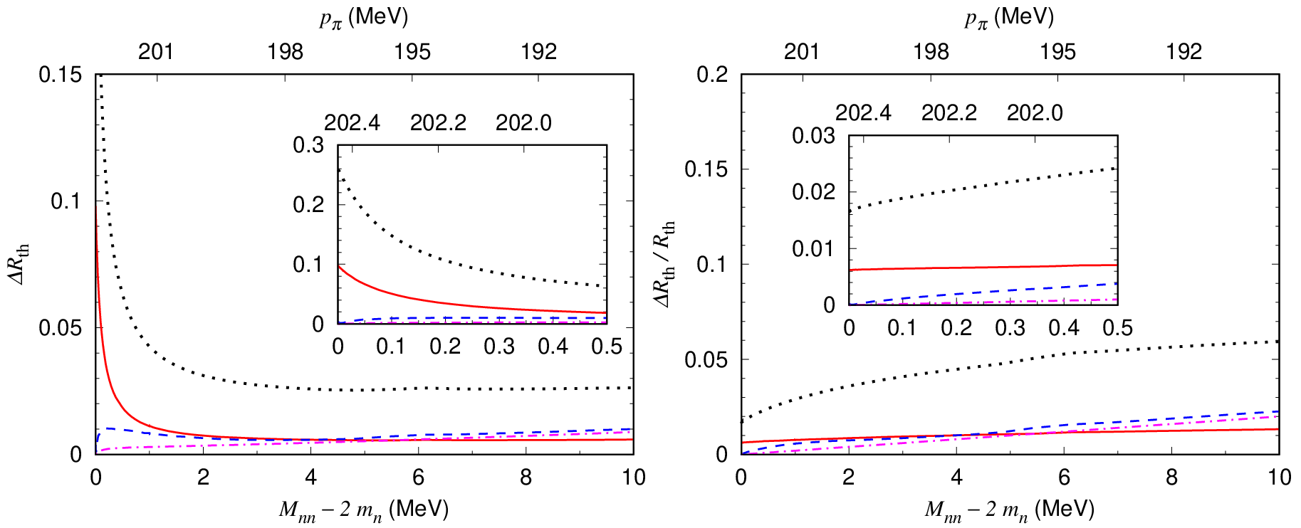
where $t^{\rm ERE}_{NN,NN}$ is the $NN$ amplitude parametrized with the effective range expansion of Eq. (1) without the $O(p^{4})$ contribution. The result obtained with this replacement is shown in Fig. 8(left). Within the considered high-precision $NN$ potentials, the off-shell effect is very similar. To clarify the model dependence, the ratios of the curves in Fig. 8(left) divided by the one from the CD-Bonn potential are shown in Fig. 8(right). We also calculate the $NN$ off-shell uncertainty of $R_{\rm th}$ using Eq. (16) with $N_{\rm model}=3$ for the Nijmegen I, II, and Reid93 potentials. The calculated $\Delta R_{\rm th}$ is represented by the red solid curve in Fig. 9(left). The variation of the shape of $R_{\rm th}$ due to the uncertainty could be seen more clearly in $\Delta R_{\rm th}/R_{\rm th}$, as shown in Fig. 9(right). From the figure, we can see that the uncertainty of the $NN$ off-shell effect on $R_{\rm th}$ is less than 1.5% (1%) for $M_{nn}-2m_{n}\leq 10$ MeV (0.5 MeV).

The uncertainty of the elementary $\gamma p\to\pi^{+}n$ amplitudes may affect the theoretically calculated $M_{nn}$ distribution. This uncertainty could be examined via comparing calculations with different amplitude models. We use the same DCC model as before and also the Chew-Mandelstam (CM12) parametrization cm12. The CM12 parametrization is a $K$-matrix fit to the $\gamma N\to\pi N$ data and, by construction, has only on-shell amplitudes. Thus, for comparison, we also use the on-shell DCC amplitudes. As shown in Fig. 10(left), the $M_{nn}$ distributions of $\gamma d\to\pi^{+}nn$ at $E_{\gamma}=250$ MeV are calculated with the DCC and CM12 elementary on-shell amplitudes. In this particular kinematics ($\theta_{\pi}=0^{\circ}$ and $M_{nn}\sim 2m_{n}$), the cross sections obtained with the DCC model are slightly smaller than those obtained with the CM12 solution. This reasonable agreement occurs because both the DCC model and CM12 parametrization well reproduce the $\gamma p\to\pi^{+}n$ data. Furthermore, the slight difference seen in Fig. 10(left) is almost perfectly removed in the ratio $R_{\rm th}$, as shown in Fig. 10(right). This demonstrates that by analyzing $R_{\rm th}$ and its experimental counterpart, we can study low-energy $nn$ scattering without being influenced by the uncertainty associated with on-shell elementary $\gamma p\to\pi^{+}n$ amplitudes. The uncertainty of $R_{\rm th}$ due to the on-shell $\gamma p\to\pi^{+}n$ amplitudes is calculated using Eq. (16) with $N_{\rm model}=1$ for the CM12, as shown in Fig. 9 by the blue dashed curve.

Figure 11: (Left) The $M_{nn}$ distributions at $E_{\gamma}=250$ MeV with and without the off-shell effects from the $\gamma p\to\pi^{+}n$ amplitudes. The red solid curve represents the original calculation, and the blue dashed curve is obtained by replacing the off-shell amplitudes with on-shell ones. (Right) Ratios of the curves in the left panel. Each of the curves is divided by the red solid curve in the left panel and is shown with the same feature.

In the loop diagrams, the elementary $\gamma p\to\pi^{+}n$ amplitudes also induce uncertainty associated with their off-shell effects. Although the off-shell behavior of the DCC model has been constrained by fitting data to some extent, some uncertainty would still exist. Thus, we study the off-shell effect by using the on-shell elementary amplitudes in Eqs. (6) and (7) and comparing the $R_{\rm th}$ from this calculation with the original value that considers the off-shell effect. The result is shown in Fig. 11. We observe that the off-shell effect reduces the $R_{\rm th}$ and, thus, the cross sections by 1.7%–2.4% in $M_{nn}-2m_{n}\leq 0.5$ MeV and 4.0%–6.0% in 2 MeV $<M_{nn}-2m_{n}\leq 6$ MeV. The uncertainty of $R_{\rm th}$ is difficult to estimate because an off-shell $\gamma p\to\pi^{+}n$ amplitude from a different model is not available; hence, we cannot study the model dependence. Therefore, we make a conservative estimate of the uncertainty due to the off-shell effects using Eq. (16) with $N_{\rm model}=1$ for the calculation with the on-shell DCC $\gamma p\to\pi^{+}n$ amplitudes. The result is shown in Fig. 9 by the black dotted curve.

Another source of theoretical uncertainty is the contributions from meson-exchange currents aside from those included in Fig. 2(c) and not considered in the present model. Previous research on near-threshold $\gamma d\to\pi^{+}nn$ based on the chiral perturbation theory prev also did not consider such mechanisms because they are higher-order effects within their counting scheme. As we deal with the reactions at significantly higher photon energies, their argument does not necessarily apply to our case. A previous chiral perturbation theory calculation of $\pi^{-}d\to nn\gamma$ anders considered more meson-exchange currents. However, it was found that meson-exchange currents that can be accommodated by Fig. 2(c) provide a leading effect. Therefore, we expect that the meson-exchange current missing in our calculation provides a few % contributions to the cross sections but the change in the shape would be even smaller. Thus, we assume that the missing meson-exchange current linearly increase the $R_{\rm th}(M_{nn})$ of the standard setting as $R^{1}_{\rm th}(M_{nn})=(1+0.002\,(M_{nn}-2m_{n})/{\rm MeV})\times R_{\rm th}(M_{nn})$. We then estimate the uncertainty of $\Delta R_{\rm th}$ using Eq. (16), as shown in Fig. 9 by the magenta dash-dotted curve.

Let us summarize the various theoretical uncertainties shown in Fig. 9. The largest uncertainty is from the off-shell effects of the elementary $\gamma p\to\pi^{+}n$ amplitudes shown by the black dotted curve, and it can change $R_{\rm th}$ by $\ \raise 1.29167pt\hbox{$<$\kern-7.5pt\lower 4.30554pt\hbox{$\sim$}}\ 6$%. The other uncertainties are mostly $\ \raise 1.29167pt\hbox{$<$\kern-7.5pt\lower 4.30554pt\hbox{$\sim$}}\ 2$% effects on $R_{\rm th}$. All the uncertainties are smaller in $M_{nn}-2m_{n}\leq 0.5$ MeV where $R_{\rm th}$ is sensitive to $a_{nn}$. Furthermore, the uncertainties of the line shape of $R_{\rm th}$ are generally smaller than the absolute value of $R_{\rm th}$.

Figure 12: The $M_{nn}$ distributions for different scattering length ($a_{nn}$) values. The blue dashed, black dotted, red solid, magenta dash-dotted, and green dash-two-dotted curves are calculated with $a_{nn}=-16,-17,-18,-19$, and $-20$ fm, respectively; $r_{nn}=2.75$ fm. The off-shell dependence of the $NN$ amplitudes is drawn from the CD-Bonn potential, as explained in the text. In the inlet, each $R_{\rm th}$ value is divided by the $R_{\rm th}$ of $a_{nn}=-18$ fm. The other conditions are the same as those in Fig. 3.

Figure 13: The $M_{nn}$ distributions for different effective range ($r_{nn}$) values. The blue dashed, black dotted, red solid, and magenta dash-dotted curves are calculated with $r_{nn}=1$, 2, 3, and 4 fm, respectively; $a_{nn}=-18.9$ fm. In the inlet, each $R_{\rm th}$ value is divided by the $R_{\rm th}$ of $r_{nn}=3$ fm. The other conditions are the same as those in Fig. 12.

Figure 14: Same as in Fig. 13 but for 1 MeV $\leq M_{nn}-2m_{n}\leq$ 10 MeV.

We now study the dependence of $d^{2}\sigma/d\Omega_{\pi}/dM_{nn}$ and $R_{\rm th}$ on scattering parameters $a_{nn}$ and $r_{nn}$. For this purpose, we again use Eq. (17) to calculate the $NN$ rescattering amplitudes. As discussed above, various model dependences change the absolute magnitude of $d^{2}\sigma/d\Omega_{\pi}/dM_{nn}$ and $R_{\rm th}$ by a few % levels, while their shapes remain rather stable. To extract the $a_{nn}$ and $r_{nn}$ at the precision of $\ \raise 1.29167pt\hbox{$<$\kern-7.5pt\lower 4.30554pt\hbox{$\sim$}}\ 0.5$ fm, which is comparable to previous determinations huhn; gonz; wits; chen, we use only the shape of ($d^{2}\sigma/d\Omega_{\pi}/dM_{nn}$ and ) $R_{\rm th}$ to determine the scattering parameters. To start, we vary the $a_{nn}$ from $-16$ fm to $-20$ fm, with $r_{nn}=2.75$ fm fixed; the obtained $d^{2}\sigma/d\Omega_{\pi}/dM_{nn}$ and $R_{\rm th}$ are shown in Fig. 12. The effect of changing the $a_{nn}$ value is only seen in a small region of $M_{nn}-2m_{n}\ \raise 1.29167pt\hbox{$<$\kern-7.5pt\lower 4.30554pt\hbox{$\sim$}}\ 0.3$ MeV. When the $a_{nn}$ is changed by 1 fm, the cross section changes by $\sim 10$% at most at $M_{nn}\sim 2m_{n}$, and by 4%–5% ($\sim$ 0.17 $\mu$b/sr/MeV) at $M_{nn}-2m_{n}=0.07$–0.10 MeV where the cross section reaches its peak. As the shape of $d^{2}\sigma/d\Omega_{\pi}/dM_{nn}$ and, thus, $R_{\rm th}$ sensitively changes as the $a_{nn}$ value changes, fitting $R_{\rm th}$ to the corresponding data over $M_{nn}-2m_{n}\ \raise 1.29167pt\hbox{$<$\kern-7.5pt\lower 4.30554pt\hbox{$\sim$}}\ 0.3$ MeV is an efficient way to precisely determine the $a_{nn}$.

Next, we study the $r_{nn}$ dependence. Here, we vary the $r_{nn}$ from 1 fm to 4 fm, with fixed $a_{nn}=-18.9$ fm. The result for $M_{nn}-2m_{n}<0.5$ MeV is given in Fig. 13, while that for 1 MeV $<M_{nn}-2m_{n}<10$ MeV is given in Fig. 14. For the negative $a_{nn}$, the $NN$ rescattering amplitude of Fig. 2(b) becomes weaker as the positive $r_{nn}$ increases. Thus, as the $r_{nn}$ increases, the cross section reduces (increases) in the small (large) $M_{nn}$ regions wherein the $NN$ rescattering (impulse) amplitude dominates. When the $r_{nn}$ increases by 1 fm at $M_{nn}-2m_{n}\sim 0.1$ MeV, the cross section reduces by $\sim 1.5$% ($\sim$ 0.06 $\mu$b/sr/MeV). As discussed in the above paragraph, the shape of $R_{\rm th}$ is sensitive to the $a_{nn}$ in $M_{nn}-2m_{n}\ \raise 1.29167pt\hbox{$<$\kern-7.5pt\lower 4.30554pt\hbox{$\sim$}}\ 0.3$ MeV. In this $M_{nn}$ region, the shape of $R_{\rm th}$ also depends on the $r_{nn}$, as seen in the inlet of Fig. 13. If the $r_{nn}$ is in the range of $|r_{nn}-2.75\,{\rm fm}|<0.5$ fm, as expected from Eq. (2), the shape of $R_{\rm th}$ changes from that for $r_{nn}$ = 2.75 fm by less than 1%. Thus, it is important to control the $r_{nn}$ at the 0.5 fm level. Although old data were used to constrain the $r_{nn}$ (see Ref. review_slaus for review), it would be more desirable to use the $\gamma d\to\pi^{+}nn$ data to directly constrain the $r_{nn}$ at the precision of 0.5 fm, without resorting to CS. As seen in the inlet of Fig. 14(right), the shape of $R_{\rm th}$ for 2 MeV $<M_{nn}-2m_{n}<6$ MeV shows a good sensitivity to the $r_{nn}$ but no sensitivity to the $a_{nn}$.

We then perform a Monte Carlo simulation and extract the $a_{nn}$ and $r_{nn}$ with the uncertainties from $R_{\rm exp}$, an experimental counterpart to $R_{\rm th}$, under several realistic settings, such as different finite $M_{nn}$ bin widths and different precisions of $R_{\rm exp}$. The $R_{\rm exp}$ data are generated with the fixed values of $a_{nn}^{\circ}$ and $r_{nn}^{\circ}$. Specifically, we perform a procedure defined by the following four steps:

1. We introduce: $R^{\circ}_{\rm exp}(a_{nn}^{\circ},r_{nn}^{\circ};M_{nn})\equiv R_{\rm th}(a_{nn}^{\circ},r_{nn}^{\circ};M_{nn})+g\Delta R_{\rm th}^{\rm all}(M_{nn})$ where $\Delta R_{\rm th}^{\rm all}(M_{nn})$ is the quadratic sum of $\Delta R_{\rm th}(M_{nn})$s from different sources, as shown in Fig. 9(left). The parameter $g$ is randomly generated at each cycle according to the standard normal distribution.

2. The histogram $R^{\circ}_{\rm exp}(a_{nn}^{\circ},r_{nn}^{\circ};i)$ for the $i$-th bin is created by averaging $R^{\circ}_{\rm exp}(a_{nn}^{\circ},r_{nn}^{\circ};M_{nn})$ with respect to $M_{nn}$ over the bin width.

3. The histogram data $R_{\rm exp}(i)$ are generated from $R^{\circ}_{\rm exp}(i)$ via including a statistical fluctuation corresponding to the given precision.

4. We simultaneously search for the $a_{nn}$ and $r_{nn}$ with which $R_{\rm exp}(a_{nn},r_{nn};M_{nn})$, averaged over the bin width, optimally fits $R_{\rm exp}(i)$ in the $M_{nn}$ range of [0.00, 6.00) MeV. We can multiply a free overall coefficient to $R_{\rm exp}(a_{nn},r_{nn};M_{nn})$, as we just attempt to reproduce the shape.

The above procedure is repeated 10,000 times, and the width of the obtained $a_{nn}$ ($r_{nn}$) distribution corresponds to the uncertainty. This analysis is performed with several different values of $a_{nn}^{\circ}$ and $r_{nn}^{\circ}$ over $-20$ fm $\leq a_{nn}^{\circ}\leq-15$ fm and 1 fm $\leq r_{nn}^{\circ}\leq 5$ fm. The centroid values of the $a_{nn}$ and $r_{nn}$ well reproduce $a_{nn}^{\circ}$ and $r_{nn}^{\circ}$. The $a_{nn}$ uncertainty is approximately proportional to the $R_{\rm exp}$ precision. When the $M_{nn}$ bin width is 0.04 MeV, a precision of 5% is required to lower the $a_{nn}$ uncertainty to less than 0.5 fm. With the same bin width, the $r_{nn}$ uncertainty is $\ \raise 1.29167pt\hbox{$<$\kern-7.5pt\lower 4.30554pt\hbox{$\sim$}}\ 0.1$ fm ($\sim$ 0.05 fm) for the precision of 5% (0%). A smaller bin width results in a smaller $a_{nn}$ uncertainty ($\Delta a_{nn}=0.13$–0.27 fm for the bin width of 0.01–0.08 MeV and 2% precision) but a larger $r_{nn}$ uncertainty ($\Delta r_{nn}=0.23$–0.06 fm for the bin width of 0.01–0.08 MeV and 2% precision) owing to the theoretical uncertainties of $\Delta R_{\rm th}$s. These results do not change very much within the specified range of $a_{nn}^{\circ}$. When we use $a_{nn}^{\circ}=-18.9$ fm and $r_{nn}^{\circ}=2.75$ fm, we obtain $\Delta a_{nn}=0.21$ fm and $\Delta r_{nn}=0.06$ fm for an 0.04 MeV bin width and $\pm 2\%$ precision of $R_{\rm exp}$ in each bin. By comparing the results obtained with and without $\Delta R_{\rm th}^{\rm all}$, we find that $\Delta a_{nn}$(theory)=0.03 fm and $\Delta r_{nn}$(theory)=0.06 fm due to $\Delta R_{\rm th}^{\rm all}$ contribute to $\Delta a_{nn}$ and $\Delta r_{nn}$ through the quadratic sum.

IV Experimental strategy used to extract high-resolution $\gamma d\to\pi^{+}nn$ data from pion electroproduction data

In this section, we discuss how we experimentally obtain high-resolution $M_{nn}$ distribution data of $\gamma d\to\pi^{+}nn$ to determine the $nn$ scattering parameters. Since we do not detect neutrons, the momenta and angles of the photon and pion have to be measured with sufficiently high resolutions. Considering the currently available experimental facilities around the world, we cannot achieve such high resolutions with a real photon beam. However, we can achieve a high $M_{nn}$ resolution utilizing virtual photons ($\gamma^{*}$s) from electron scattering and two magnetic spectrometers to detect the scattered electrons and emitted positive pions. Upon tuning the electron scattering kinematics, we can measure cross sections for pion production with a so-called “almost-real” photon at a low momentum transfer ($Q^{2}\sim 0$).

The triple-differential unpolarized cross section for the $d(e,e^{\prime}\pi^{+})nn$ reaction is written as follows (differentiation with respect to $M_{nn}$ being omitted):

$$\frac{d^{3}\sigma^{e\,d}}{dE_{e^{\prime}}\,d\Omega_{e^{\prime}}\,d\Omega_{\pi}}=\Gamma_{\gamma}\left(\frac{d\sigma_{\rm T}}{d\Omega_{\pi}}+\epsilon_{\rm L}\frac{d\sigma_{\rm L}}{d\Omega_{\pi}}+\sqrt{2\epsilon_{\rm L}\left(1+\epsilon\right)}\frac{d\sigma_{\rm LT}}{d\Omega_{\pi}}\cos\phi_{\pi}+\epsilon\frac{d\sigma_{\rm TT}}{d\Omega_{\pi}}\cos 2\phi_{\pi}\right),$$ (18)

where the electron mass is neglected, and $\sigma_{\rm T}$, $\sigma_{\rm L}$, $\sigma_{\rm LT}$, and $\sigma_{\rm TT}$ are the transverse, longitudinal, longitudinal-transverse interference, and transverse-transverse interference cross sections for $\gamma^{*}d\to\pi^{+}nn$ in the laboratory frame, respectively forest; mulders. The pion angle $\Omega_{\pi}=(\theta_{\pi},\phi_{\pi})$ is measured with respect to the virtual photon direction, and $\phi_{\pi}$ is the angle between the electron-scattering $(e,e^{\prime})$ plane and the pion-production $(\gamma^{*},\pi)$ plane. We denote the incident (scattered) electron energy and momentum in the laboratory frame by $E_{e}$ and $\bm{p}_{e}$ ($E_{e^{\prime}}$ and $\bm{p}_{e^{\prime}}$), respectively, and the electron scattering angle by $\cos\theta_{e^{\prime}}=\left(\bm{p}_{e}\cdot\bm{p}_{e^{\prime}}\right)/\left(|\bm{p}_{e}||\bm{p}_{e^{\prime}}|\right)$. Also, the four-momentum transfer from the electron to the deuteron is denoted by $(\omega,\bm{q})=(E_{e}-E_{e^{\prime}},\bm{p}_{e}-\bm{p}_{e^{\prime}})$ and the squared momentum transfer by $Q^{2}=-\left(\omega^{2}-\left|\bm{q}\,\right|^{2}\right)$. With these notations, we introduced in Eq. (18)

$$\epsilon=\left(1+\frac{2\left|\bm{q}\,\right|^{2}}{Q^{2}}\tan^{2}\frac{\theta_{e^{\prime}}}{2}\right)^{-1}\quad{\rm and}\quad\epsilon_{\rm L}=\frac{Q^{2}}{\omega^{2}}\epsilon\ ,$$ (19)

and the virtual photon flux given by

$$\Gamma_{\gamma}=\frac{\alpha}{2\pi^{2}Q^{2}}\frac{E_{\gamma}}{1-\epsilon}\frac{E_{e^{\prime}}}{E_{e}}\ ,$$ (20)

with $\alpha$ as the fine structure constant, and $E_{\gamma}=\omega-Q^{2}/2m_{d}$ as the photon equivalent energy in the laboratory frame with which a real photon excites a deuteron to a hadronic system with the same invariant mass as a virtual photon with the four-momentum $q$ does. The virtual photon emission angle $\theta_{\gamma}$ is specified by $\cos\theta_{\gamma}=\left(\bm{p}_{e}\cdot\bm{q}\right)/\left(|\bm{p}_{e}||\bm{q}|\right)$. In Eq. (18), all cross sections depend on $E_{\gamma}$ and $Q^{2}$, and $d\sigma_{\rm T}/d\Omega_{\pi}(Q^{2}=0)$ differentiated with respect to $M_{nn}$ corresponds to Eq. (4).

The elementary $\gamma N\to\pi N$ data [$d\sigma^{\gamma N}_{\rm T}/d\Omega_{\pi}(Q^{2}=0)$] are generally more precisely measured than $\gamma^{*}N\to\pi N$ data [$d\sigma^{\gamma^{*}N}_{\rm T}/d\Omega_{\pi}(Q^{2}\neq 0)$] from pion electroproductions. A primary reason for this is that an uncertainty enters into the data when separating $d\sigma^{\gamma^{*}N}_{\rm T}/d\Omega_{\pi}$ from $d\sigma^{\gamma^{*}N}_{\rm L}/d\Omega_{\pi}$, $d\sigma^{\gamma^{*}N}_{\rm LT}/d\Omega_{\pi}$, and $d\sigma^{\gamma^{*}N}_{\rm TT}/d\Omega_{\pi}$. Consequently, the $Q^{2}=0$ sector of the DCC model, as well as other similar models for $\gamma^{(*)}N\to\pi N$, is significantly better tested by the real photon data, in comparison with the finite $Q^{2}$ sector of the models. Therefore, for a reliable determination of $nn$ scattering parameters using such models, almost-real photon data of $\gamma d\to\pi^{+}nn$, i.e., $d\sigma_{\rm T}/d\Omega_{\pi}$ in Eq. (18) at $Q^{2}\sim 0$, are highly preferred.

Here, we consider a method to extract $d\sigma_{\rm T}/d\Omega_{\pi}$ at $Q^{2}\sim 0$ from the $d(e,e^{\prime}\pi^{+})nn$ cross sections. The $d\sigma_{\rm LT}/d\Omega_{\pi}$ and $d\sigma_{\rm TT}/d\Omega_{\pi}$ terms in Eq. (18) vanish at $\theta_{\pi}=0$ because they are proportional to $\sin\theta_{\pi}$ and $\sin^{2}\theta_{\pi}$, respectively. Fortunately, the $\gamma d\to\pi^{+}nn$ data at $\theta_{\pi}=0$ are exactly what we need, as discussed in connection with Fig. 6. Now, Eq. (18) at $\theta_{\pi}=0$ is simplified:

$$\frac{d^{3}\sigma^{e\,d}}{dE_{e^{\prime}}\,d\Omega_{e^{\prime}}\,d\Omega_{\pi}}=\Gamma_{\gamma}\left(\frac{d\sigma_{\rm T}}{d\Omega_{\pi}}+\epsilon_{\rm L}\frac{d\sigma_{\rm L}}{d\Omega_{\pi}}\right).$$ (21)

The $\epsilon_{\rm L}d\sigma_{\rm L}/d\Omega_{\pi}$ contribution can be made smaller by using the kinematics wherein $\epsilon_{\rm L}$ and $Q^{2}$ are low. Even when the $\epsilon_{\rm L}d\sigma_{\rm L}/d\Omega_{\pi}$ contribution cannot be made negligible, we can still separate out ${d\sigma_{\rm T}}/{d\Omega_{\pi}}$ utilizing the linear $\epsilon_{\rm L}$ dependence in Eq. (21).

The A1 spectrometer facility at Mainz Microtron (MAMI) spek is an outstanding candidate to conduct an experiment under the above-mentioned kinematic and precision conditions. The facility is capable of providing high energy-resolution electron beams ($\delta p/p<10^{-4}$) and measuring the momenta and angles of electrons and pions with the high resolutions, i.e., $\delta p/p=10^{-4}$ and $\delta\theta<3$ mrad ($0.2^{\circ}$), required to determine the $nn$ scattering parameters. Three magnetic spectrometers, i.e., SpekA, SpekB, and SpekC, are placed in a horizontal plane ($\phi_{\pi}=0^{\circ}$). SpekA and SpekC, each of which covers $\pm 100$ mrad ($\pm 5.7^{\circ}$), can be placed from $18^{\circ}$ to $160^{\circ}$ from the primary electron beam direction. SpekB can be placed at more forward angles from $7^{\circ}$ to $62^{\circ}$ and has a relatively smaller coverage of $\pm 20$ mrad ($\pm 1.1^{\circ}$). Table 1 briefly lists the parameters of these three spectrometers at MAMI.

Table 1: Summary of the parameters of the three spectrometers at MAMI. These parameters are taken from Ref. spek.

spectrometer	SpekA	SpekB	SpekC
minimum angle	$18^{\circ}$	$7^{\circ}$	$18^{\circ}$
maximum angle	$160^{\circ}$	$62^{\circ}$	$160^{\circ}$
horizontal angular coverage (mrad)	$\pm 100$	$\pm 20$	$\pm 100$
vertical angular coverage (mrad)	$\pm 70$	$\pm 70$	$\pm 70$
angular resolution at the target position (mrad)	$<3$	$<3$	$<3$
momentum bite	$\pm 20\%$	$\pm 15\%$	$\pm 25\%$
momentum resolution ($\delta p/p$)	$10^{-4}$	$10^{-4}$	$10^{-4}$

The experimental constraints do not allow us to use a kinematical setting wherein $\epsilon_{\rm L}d\sigma_{\rm L}/d\Omega_{\pi}$ is negligible compared with $d\sigma_{\rm T}/d\Omega_{\pi}$. Thus, a realistic solution is to separate the $d\sigma_{\rm T}/d\Omega_{\pi}$ and $d\sigma_{\rm L}/d\Omega_{\pi}$ contributions by taking advantage of the linear $\epsilon_{\rm L}$ dependence in Eq. (21). For this purpose, we need to measure cross sections at several kinematical points wherein $\omega$ and $Q^{2}$, thus, $d\sigma_{\rm T}/d\Omega_{\pi}$ and $d\sigma_{\rm L}/d\Omega_{\pi}$ are the same, while $\epsilon_{\rm L}$ is different. In addition, the $Q^{2}$ has to be low enough to regard the virtual photon as real. Suppose we utilize SpekA and SpekB to detect the scattered electrons and emitted positive pions, respectively. To obtain $E_{\gamma}=200$ (250) MeV under the constraints of $\theta_{e^{\prime}}\geq 12.3^{\circ}$ and $\theta_{\gamma}\geq 5.9^{\circ}$, the minimum $Q^{2}$ achievable is 0.0021 (0.0013) GeV${}^{2}/c^{2}$ and $\epsilon_{\rm L}=1.92\%$. At this $Q^{2}$ value, the experimental constraints would not allow us to change $\epsilon_{\rm L}$; thus, the $\sigma_{\rm T}$-$\sigma_{\rm L}$ separation is impossible. To cover a wide range of $\epsilon_{\rm L}$ for the separation, we choose $Q^{2}=0.0050$ GeV${}^{2}/c^{2}$. To use the virtual photon of $Q^{2}=0.0050$ GeV${}^{2}/c^{2}$ and $E_{\gamma}=200$ or 250 MeV, relations between the kinematical electron and photon variables ($E_{e}$, $E_{e^{\prime}}$, $\theta_{e^{\prime}}$, $\epsilon_{\rm L}$, and $\theta_{\gamma}$) are shown in Fig. 15. The experimental constraint of $\theta_{\gamma}\geq 5.9^{\circ}$ requires $E_{e}\geq 230$ (300) MeV for $E_{\gamma}=200$ (250) MeV, producing $\epsilon_{\rm L}\geq 2.24\%$ (2.17%). The $d(e,e^{\prime}\pi^{+})nn$ cross sections measured at several electron kinematics in Fig. 15 are used for the $\sigma_{\rm T}$-$\sigma_{\rm L}$ separation, providing $d\sigma_{\rm T}/d\Omega_{\pi}$ at $Q^{2}=0.0050$ GeV${}^{2}/c^{2}$.

Figure 15: (a) Incident electron energy $E_{e}$ (blue solid line) and scattered electron energy $E_{e^{\prime}}$ (red dashed line) as a function of the emission angle of virtual photons in the laboratory frame $\theta_{\gamma}$ at $Q^{2}=0.0050$ GeV${}^{2}/c^{2}$ for $E_{\gamma}=200$ MeV (left) and 250 MeV (right). (b) Electron scattering angle $\theta_{e^{\prime}}$. (c) Degree of longitudinal polarization $\epsilon_{\rm L}$.

Note that within the $\gamma d\to\pi^{+}nn$ model used in this work, $d\sigma_{\rm T}/d\Omega_{\pi}$ at $Q^{2}=0$ is slightly larger by $\sim 1$% than that at $Q^{2}=0.0050$ GeV${}^{2}/c^{2}$, and the shape of the $M_{nn}$ distribution hardly changes. Therefore, we can directly apply the analysis method and results for the real photon presented in the previous sections to the data of $d\sigma_{\rm T}/d\Omega_{\pi}$ at $Q^{2}=0.0050$ GeV${}^{2}/c^{2}$ to determine the $nn$ scattering parameters. Additionally, due to the high angle resolution ($<$ 3 mrad) of the facility, we do not need to modify the presented results in which the finite angle resolution is not accounted for.

V Summary

In this paper, we discussed the possibility of extracting the low-energy neutron-neutron scattering parameters of $a_{nn}$ and $r_{nn}$ from $\gamma d\to\pi^{+}nn$ cross-section data. The analysis was based on a theoretical model of $\gamma d\to\pi^{+}nn$ that incorporated realistic elementary amplitudes for $\gamma p\to\pi^{+}n$, $NN\to NN$, and $\pi N\to\pi N$. We demonstrated that $\gamma d\to\pi^{+}nn$ at the special kinematics with $\theta_{\pi}=0^{\circ}$ and $E_{\gamma}\sim 250$ MeV is suitable for studying neutron-neutron scattering in a low $nn$ invariant mass region ($M_{nn}\sim 2m_{n}$) because the $NN$ rescattering mechanism dominates while the $\pi N\to\pi N$ rescattering contribution is negligible. We assessed theoretical uncertainties from various sources, including the on- and off-shell behaviors of the $\gamma p\to\pi^{+}n$ and $NN\to NN$ amplitudes. This assessment showed that the shape of the ratio $R_{\rm th}$, defined with the $\gamma d\to\pi^{+}nn$ cross section ($d^{2}\sigma/dM_{nn}/d\Omega_{\pi}$) as in Eq. (13), was particularly useful for extracting the $a_{nn}$ and $r_{nn}$ from data because it had a good sensitivity to these scattering parameters and significantly reduced the model dependences compared with $d^{2}\sigma/dM_{nn}/d\Omega_{\pi}$. The experimental counterpart to $R_{\rm th}$, $R_{\rm exp}$, is defined with measurable $\gamma d\to\pi^{+}nn$ and $\gamma p\to\pi^{+}n$ cross sections and the deuteron wave function. Through a Monte Carlo simulation, we found that $R_{\rm exp}$ with 2% error, resolved into an $M_{nn}$ bin width of 0.04 MeV, could determine $a_{nn}$ and $r_{nn}$ values with uncertainties of $\pm 0.21$ fm and $\pm 0.06$ fm, respectively, if $a_{nn}=-18.9$ fm and $r_{nn}=2.75$ fm. The uncertainties did not significantly change when the $a_{nn}$ value was changed from $-20$ to $-15$ fm. Such a high $M_{nn}$ resolution can be achieved with an electron scattering experiment that utilizes the A1 spectrometer facility at MAMI. The $d^{2}\sigma/dM_{nn}/d\Omega_{\pi}$ for $d(\gamma,\pi^{+})nn$ can be separated from the $d^{4}\sigma/dE_{e^{\prime}}/d\Omega_{e^{\prime}}/dM_{nn}/d\Omega_{\pi}$ for $d(e,e^{\prime}\pi^{+})nn$ at different $\epsilon_{\rm L}$ values but the same $Q^{2}\simeq 0$ (an almost-real photon condition). Since the proposed method does not require the difficult experimental task of handling neutron detection efficiency and its uncertainty, it has a great advantage over the previous method that extracted the $a_{nn}$ from the neutron time-of-flight spectrum of $\pi^{-}d\to\gamma nn$.