Technological interdependencies predict innovation dynamics

Abstract

We propose a simple model where the innovation rate of a technological domain depends on the innovation rate of the technological domains it relies on. Using data on US patents from 1836 to 2017, we make out-of-sample predictions and find that the predictability of innovation rates can be boosted substantially when network effects are taken into account. In the case where a technology’s neighborhood future innovation rates are known, the average predictability gain is 28% compared to simpler time series model which do not incorporate network effects. Even when nothing is known about the future, we find positive average predictability gains of 20%. The results have important policy implications, suggesting that the effective support of a given technology must take into account the technological ecosystem surrounding the targeted technology.

1 Introduction

Technological evolution is often described as a recursive process whereby the recombination of existing components leads to new or improved technological components (Schumpeter, 1939; Usher, 1954; Kauffman, 1993; Fleming, 2001; Arthur, 2009; McNerney et al., 2011; Tria et al., 2014; Youn et al., 2015; Fink and Reeves, 2019). A simple hypothesis, therefore, is that technological domains that tend to recombine elements from fast-growing technological domains should themselves grow faster. In other words, a technology will tend to progress faster if the technologies it relies on are themselves making fast progress. While these ideas are well established, very little has been done to establish empirically that technological interdependencies help predict future innovation dynamics. Being able to demonstrate this relationship would be very helpful, as it would allow us to support key technologies and overall technological progress by designing and supporting technological ecosystems.

In this paper, we establish that knowing the technological ecosystem helps predict the dynamics of future innovation. We use a simple model where the innovation rates of a technological domain depends on efforts within the domain, but also on the stock of knowledge in the domain and in supporting domains. We test the model on the record of United States Patent Office (USPTO) patents from 1836 to 2017, which includes more than 10M patents, 40M classifications in $\sim 650$ technological domains, and 90M citations. As predicted by the model, we find that that the growth rates of the number of patents in a technological domain depends strongly on the growth rates of its knowledge sources. Given the volatile nature of growth rates, this strong relationship is remarkable. We use this insight for making out-of-sample predictions of patenting activities and find that integrating network effects can improve predictions substantially compared to independent time series models. The results have important policy implications, suggesting that research policy targeted at fostering innovation in a technological domain has to take its surrounding technological ecosystem into account.

Several studies have put forward the idea of network-dependent innovation dynamics. For instance, Cowan and Jonard (2003) and König et al. (2011) have proposed models of innovation arising from the recombination of knowledge in R&D partnership networks.

Acemoglu et al. (2016) find that upstream patenting levels are highly correlated with downstream patenting levels. Taalbi (2018) finds broadly similar results using innovation counts and a network constructed to reflect which industry uses innovation from another industry. Patenting levels are persistent, and so are automatically very predictable. In contrast, we focus on changes in patenting levels, which are not persistent and are much more difficult to predict.

Our work on innovation dynamics is also related to evolutionary models such as Farmer et al. (1986), Bagley et al. (1992) and Jain and Krishna (2001). In these models, the exponential growth trajectories of nodes arise due to the existence of autocatalytic sets, i.e. a subset of the network where nodes have at least one positive incoming link from a node of the same subgraph, leading to sustainable self-reinforcing dynamics. Evidence for the presence of autocatalytic sets in technology systems was recently provided by Napolitano et al. (2018) who find that the autocatalytic structure of the patent network has grown in time and that patent classes belonging to the autocatalytic set show higher levels of innovation activity.

Our contribution to the literature can be summarized as follows. First, we show strong empirical evidence of coupled innovation growth in the presence of network linkages and demonstrate that the observed effects are far from what would be expected by chance (Section 2). Second, we propose a simple theoretical model of network-dependent knowledge production which is able to explain the observed empirical pattern. We then show how the model can be estimated from empirical data, and quantify how network effects in innovation dynamics have become more important over the last 70 years (Section 3). Finally, we validate the model by predicting future patenting levels (Section 4). We find that independent time series models can be substantially improved in case network information is available.

2 Empirical evidence

Figure 1: a) Technologies’ 10-year growth rates $g$ for the horizon 2000 to 2010 plotted against average nearest neighbor growth rates $\tilde{g}$ (ANNG). The neighbors’ growth rates are calculated based on the technology network in 2000. The plot thus suggests that technologies experienced a similar growth rate over the next ten year as the technologies they were linked to in 2000. b) Network assortativity over time with respect to 1-year (upper panel), 5-year (center panel) and 10-year (bottom panel) growth rates. There is pronounced correlation between growth rates of nodes and their neighbors in the technology network, while the randomized assortativity measure hovers around zero. The shaded area around the randomized network predictions depict the 0.05-0.95 quantile range of the 1,000 sample realizations. The correlations tend to get stronger in time in the empirical network.

2.1 Data and network construction

We use data on the whole universe of granted United States patents starting in 1836 up to 2017, where the year refers to the publishing date of the patent. The dataset covers 9.83 million patents and over 91 million citations. Each patent is categorized by the patent office into one of several Cooperative Patent Classification (CPC) codes. We regard each 4-digit CPC code as a distinct technological domain. We construct a directed network $C_{t}$ where an element $C_{ij,t}$ is the sum of all citations from technology $j$ at time $t$ to technology $i$. In A we show how this matrix can be derived from patent citations by straightforward algebra. In our analysis, we use row-normalized matrices $\{W_{t}:t=1947,...,2017\}$ where each element $W_{ij,t}$ is defined as

$${W}_{ij,t}:=\frac{C_{ij,t}}{\sum_{j=1}C_{ij,t}}.$$ (1)

Thus, the row $\{W_{ij,t}:j=1\dots N\}$ can be interpreted as technology $i$’s dependence in its patenting activity at time $t$ on all other technologies: each entry is the share of citations from technology $i$ at time $t$ to another technological domain $j$. This is a temporal network with yearly snapshots (Masuda and Lambiotte, 2016). We do not construct networks for years before 1947, because earlier citations made by patents are not well documented. But citations to earlier patents are well reported. For example, a citation from a patent granted after 1947 to a patent of the 19${}^{\text{th}}$ century is included in the network.

2.2 Preliminary evidence

We now investigate whether technological domains connected to fast-growth technological domains also grow faster. In other words, we study the assortativity of the temporal network with respect to patenting growth rates. For each technology, we compute its neighborhood patenting growth rate as the average nearest neighbor growth rate (ANNG),

$$\tilde{g}_{i,t}=\sum_{j=1}^{N}\frac{C_{ij,t}(1-\delta_{ij})}{\sum_{k=1}C_{ik,t}(1-\delta_{ik})}g_{j,t},$$ (2)

where $\delta_{ij}$ denotes the Kronecker delta (the matrix diagonal is excluded in the summation so that the ANNG measures neighbor growth rates only). We then test if there is a positive correlation between growth rates of patenting activity in technological domains and their ANNG.

Fig. 1a) plots the 10-year growth rates against the 10-year ANNG for the technology network in 2000, revealing a highly significant positive relationship in growth rates from 2000 to 2010 between technologies and their neighborhood. Since the technology network is based on the year 2000, the figure suggests that if a technology draws a significant share of knowledge from another technology in 2000, we would expect them to exhibit similar growth rates over the next ten years. This pronounced positive relationship is striking given that it is based on growth rates, which tend to be much noisier than patenting levels. While one could expect the network to be assortative with respect to degrees and patenting levels, assortativity with respect to growth rates is far less trivial.

Although interesting, we should test if this relationship holds over time and if we really can be sure that the observed relationship is significantly different from what a null model would produce. To benchmark our results, we calculate the correlations between growth rates and ANNG rates for a randomized version of the given technology network. For each year $t$ and a fixed row $i$ in the matrix ${W}_{t}$, we resample all off-diagonal entries without replacements. In the randomized control network the nodes still have the same weighted outgoing links, but now randomly pointing to other nodes (excluding self-loops). We repeat the randomization process 1,000 times and report the average correlation between growth rates and ANNG as the corresponding null model. Fig. 1b) plots the Pearson correlation over time between growth rates and ANNG, once computed in the given technology network and once in the randomized control. We report the results for three different growth rates, 1-year (upper panel), 5-year (center panel) and 10-year growth rates (bottom panel). The positive correlation structure between knowledge sources growth and own growth rates over time is far from what one would expect from a network where nodes distribute their out-links randomly over the whole set of potential knowledge sources. Intuitively, one would expect that network effects materialize over the long run instead of showing immediate effects. The figure confirms this hypothesis, but even for 1-year growth rates we find relatively strong and significant positive correlations. Another interesting aspect is that for all three growth rate types, the positive relationship tends to get stronger over time. Further evidence on the impact of a technology’s neighborhood on its patenting dynamics is discussed in the supplementary information.

3 Network-dependent knowledge creation

3.1 The model

To explain the empirical observations, we now introduce a simple model of network-dependent knowledge creation and discuss its implications for the long-term evolution of technologies. Let us consider $N$ distinct technological domains. The creation of new knowledge in a technological domain requires active research effort, and depends positively on the existing stock of knowledge, from the same domain or from specific other domains.

More precisely, we assume that the creation of new knowledge follows the dynamical system

$$\dot{K}_{i}(t)=\theta_{i}R_{i}(t)^{\alpha}\prod_{j=1}^{N}K_{j}(t)^{\beta W_{ij}},$$ (3)

where $\theta_{i}$ is a technology-specific productivity parameter, $R_{i}(t)$ the research effort in domain $i$ at time $t$ and ${K}_{i}(t)$ is the stock of knowledge in $i$ at $t$. The technological ecosystem is represented by the weighted adjacency matrix $W$ which is normalized to be row-stochastic and for mathematical convenience assumed to be fixed in time. A technological domain is then a node in the network whose innovation rates depend on its location in the technological ecosystem. If a technology $i$ draws knowledge from the knowledge stock of node $j$ in the innovation process, the two nodes are connected through a directed edge from $i$ to $j$. The directed link has the weight $W_{ij}$ denoting the share of technology $j$’s knowledge in the creation of new knowledge in technology $i$. $\theta_{i}$ captures the fact that intrinsic characteristics of technologies affect how easy innovation rates can be influenced. $\alpha\geq 0$ denotes the elasticity of knowledge output with respect to research efforts. The elasticity of knowledge output in $i$ ($\dot{K_{i}}$) with respect to the knowledge stock in $j$ ($K_{j}$) is $\beta W_{ij}$, thus $\beta$ denotes the sum over all domains $j$ of these elasticities (since $\sum_{j}W_{ij}=1$).

Eq. (3) also relates to the knowledge production functions used in classical endogenous growth models (Romer (1990), Aghion and Howitt (1990), Grossman and Helpman (1991) and Jones (1995) ), but incorporates network effects. It simplifies to the standard Cobb-Douglas knowledge production function in case each technology uses only its own knowledge stock ($W=\mathbb{I}$). Similar equations have been estimated empirically within the “R&D spillovers” literature which estimates the impact of R& D in one entity on outcomes in another entity, such as countries, regions, firms, and sectors (Ertur and Koch, 2007; Hall et al., 2010; Ho et al., 2018).

Research effort is considered to be an exogenous policy variable which we assume to grow at a constant rate $R_{i}(t)=R_{i,0}e^{\lambda_{i}t}$. Dividing Eq. (3) by $K_{i}(t)$, taking logs and the derivative with respect to time, we obtain after rearranging the nonlinear autonomous system

$$\dot{g}_{i}(t)=\alpha\lambda_{i}{g}_{i}(t)+(\beta W_{ii}-1)g_{i}(t)^{2}+\beta g_{i}(t)\sum_{j=1}^{N}W_{ij}g_{j}(t)(1-\delta_{ij}),$$ (4)

where $g_{i}(t):=\dot{K}_{i}(t)/K_{i}(t)$ is the growth rate of the knowledge stock. Eq. (4) has been extensively studied without network effects in traditional endogenous growth models and in this case its dynamics are well-understood (Romer (2012), ch.3). When solving the model without network effects, the steady state growth rate (“balanced growth path”) is $g_{i}^{*}=\alpha\lambda_{i}/(1-\beta)$ which is globally stable under the standard assumption of $\beta<1$. Here, the long run-growth rate of knowledge in technology $i$ can only be increased by increasing the long-run growth rates of research efforts in the particular technology.

When network effects are included, a technology’s long-term growth path depends also on the growth rates of other technologies. By setting $\dot{g}_{i}=0$ for all $i$, we find the steady state of the form

$$g_{i}^{*}=\frac{\alpha\lambda_{i}}{1-\beta W_{ii}}+\frac{\beta}{1-\beta W_{ii}}\sum_{j=1}^{N}W_{ij}g_{j}^{*}(1-\delta_{ij}).$$ (5)

The steady state growth path for technology $i$ can be understood as a sum of two components. The first part is the idiosyncratic term, which equals the endogenous growth result without network effects. The second component suggests that the long-run growth of a technology depends positively on its neighbors’ growth rates.

To see the difference between the network-dependent model and a simple endogenous growth model version without network effects, let us assume that we could increase the constant growth rate of research effort in a technology $i$ from $\lambda_{i}$ to $\lambda_{i}^{\prime}$. Without network effects, this would simply increase the growth rate of $i$ by $\alpha(\lambda_{i}^{\prime}-\lambda_{i})/(1-\beta)$ with no impact on other technologies. Yet if network effects are included, this initial increase of $i$’s growth rate will also impact neighboring technologies which draw upon the knowledge stock of $i$, which in turn, will again affect their downstream neighbors and so on. If node $i$ points to any of the affected technologies, it will again experience a change in its growth rate and trigger the process again. We see that the convergence (if any) to the steady state after a shock in the research effort variable is more involved if the innovation rate of a technology depends on other technologies. The phase portraits depicted in Fig. 2 visualize how a change in research efforts impact innovation dynamics in a simple system of only two technologies, one with network effects (right panel) and one without (left panel).

Figure 2: Phase portraits of growth trajectories for a simple example of only two technologies. The horizontal and vertical axes denote the growth rates of technology 1 and technology 2, respectively. In the left panel there are no network effects, $W=\mathbb{I}$. In the right panel a network is present with elements $W_{ij}=0.5$ for all $i,j$. The phase diagrams are shown for initial research growth rates $\lambda_{1}=0.02$ and $\lambda_{2}=0.05$. The remaining parameters are set as follows: $\alpha=\beta=0.5$. With this parametrization all trajectories converge to the steady state $(g_{1}^{*},g_{2}^{*})=(0.02,0.05)$ in the no-network case and to the steady state $(g_{1}^{*},g_{2}^{*})=(0.0275,0.0425)$ if network effects are included. In the absence of network effects, the steady state growth rates are simply equal the research effort growth rates. If network effects are included, technology 1 is growing faster in steady state since it draws knowledge from technology 2 which experiences higher research effort growth. In contrast, for technology 2 the steady state growth rate is lower due to the network effects. The black arrows indicate how the steady state of the system moves if research effort growth $\lambda_{1}$ is doubled to $\lambda_{1}^{\prime}=0.04$, but leaving $\lambda_{2}=0.05$ unchanged. In the left panel, this increases only the steady state growth rate for technology 2, but leaves technology 2 unaffected. In the right panel where network effects are included both technologies benefit from the increase in research effort in technology 1. The red dashed line shows the trajectory of the steady state as a function of $\lambda_{1}$.

3.2 Calibration

While the dynamical system can have a non-trivial transient, for simplicity we calibrate the model based on the steady state results, using maximum likelihood. To do so, we reformulate Eq. (5) as the econometric model

$$g_{i,t}=\frac{a_{i}}{1-\beta W_{ii,t}}+\frac{\beta}{1-\beta W_{ii,t}}\sum_{j=1}^{N}W_{ij,t}g_{j,t}(1-\delta_{ij})+\epsilon_{i,t},$$ (6)

where $\epsilon_{i,t}\sim N(0,\sigma^{2})$ and $a_{i}$ is capturing the composite variable $\alpha\lambda_{i}$.

The specification is related to spatial econometric models using panel data (Elhorst, 2014; Wang and Yu, 2015), but there are also significant differences. To estimate the parameters, we therefore derive an estimator which is outlined in more detail in C. We allow the technology network to be time-varying, since we observe changing citation networks over time. In the supplementary information we present results of extensive robustness checks, covering alternative model specifications such as using time-fixed networks and spatial autoregressive models. There we also control for further possible explanatory variables, such as technological domain sizes.

The model is derived in terms of knowledge stocks $K_{i,t}=\sum_{\tau=0}^{t}P_{i,\tau}$, but knowledge stocks grow very smoothly, leaving little variance to exploit for estimating the parameters of interest. In the steady state, however, by definition growth rates are constant over time within each domain. In that case, the (deterministic) growth rates of stocks and flows are the same. Thus, for empirical convenience, we let $g_{i,t}:=\ln(P_{i,t}/P_{i,t-\tau})$ be the $\tau$-year patenting growth rate of the technology class $i$ at a time $t$.

We fit the model to the whole time series up to 2017 and report the estimated parameters in Table 1. Since the results of Section 2 suggest varying magnitudes of network effects for different time lags, we estimate the parameters for 1-year, 5-year and 10-year growth rates (columns one to three, respectively). Unsurprisingly, we find research growth parameters $a_{i}=\alpha\lambda_{i}$ which are positive on average and higher for larger time lags. The highly significant network parameter $\beta$ is large, ranging from 0.85 to 0.94, depending on the growth rate lag. This value is large, because if $\beta>1$, we would expect exploding dynamics where an increasing knowledge stock leads to ever larger growth rates. $\beta$ is smaller, but close to one, exemplifying the importance of the existing technology network for future innovation dynamics.

Dependent variable: patenting growth
	(1-y)	(5-y)	(10-y)
average $\hat{a}_{i}$	0.01	0.03	0.04
$\hat{\beta}$	0.85∗∗∗	0.93∗∗∗	0.94∗∗∗
	(0.0059)	(0.0060)	(0.0076)
$\hat{\sigma}^{2}$	0.10	0.19	0.29
Log-likelihood	-13,383	-5,464	-3,612
Observations	43,651	8,734	4,348
Note:	∗∗∗p$<10^{-16}$

Table 1: Results from estimating the econometric network model (Eq. 6). The results are shown for 1-, 5- and 10-year growth rates.

To explore the network impact on innovation growth more systematically, we rewrite the derived result in Eq. (5) into matrix notation,

$$g^{*}=\alpha L\lambda,$$ (7)

where $L:=\left[\mathbb{I}-\beta W\right]^{-1}$. The matrix representation is useful as it shows how the long-run trajectory of innovation in a given technological domain depends on the research efforts in the entire technological ecosystem. In particular, if research effort is subject to policy, we can use Eq. (7) to study two interesting policy experiments.

First, Eq. (7) allows us to identify the key supporting technologies for each technology. The naïve way to foster innovation in a technology is to increase research efforts in the particular technological domain. But Eq. (7) shows that knowledge growth depends also on research in other technologies and that there could even be cases where knowledge spillovers from research in other technologies will be more beneficial than simply devoting additional research efforts in the focal technology’s domain. Knowledge spillovers from technology $j$ to technology $i$ are made explicit when looking at the Jacobian matrix

$$\frac{\partial g^{*}_{i}}{\partial\lambda_{j}}=\alpha L_{ij}.$$ (8)

The matrix element $L_{ij}$ therefore informs us on how much we would expect the long-term innovation growth rate of technology $i$ to change as a consequence of a marginal change in technology $j$. A large row sum of off-diagonal elements $\sum_{j=1}L_{ij}(1-\delta_{ij})$ indicates a large dependence of technology $i$’s growth on external research activities. Ordering technologies based on their size in a given column yields a ranking from the most to least important supporting technologies for the focal technology.

As a second policy experiment, we can ask how a sustained change in R&D in a particular sector affects the long-run growth rate of the entire technological ecosystem. This can be relevant for a policy-maker who wants to devote her research investments in an efficient manner. For example, if a choice has to be made in what technology to invest for fostering overall innovation activities, the decision can be supported with Eq. (7). If an economy’s total knowledge is the sum of sectoral knowledge stocks $K_{tot}(t)=\sum_{i=1}^{N}K_{i}(t)$, the growth rate of the total knowledge stock can be expressed as $g_{tot}(t)=\sum_{i=1}^{N}g_{i}(t)\frac{K_{i}(t)}{K_{tot}(t)}$. The impact on total knowledge growth as a consequence of a sustained change in research effort growth in a single domain $i$ is then given by

$$\frac{\partial g^{*}_{tot}}{\partial\lambda_{j}}=\alpha\sum_{i=1}^{N}L_{ij}\frac{K_{i}}{K}+\alpha\lambda_{j}\sum_{i=1}^{N}\frac{\partial(K_{i}/K)}{\partial\lambda_{j}}L_{ij}.$$ (9)

The impact on overall innovation growth is again a sum of two components. The first part in the sum takes the form of a output multiplier, analogous to the output multiplier in input-output economics. In contrast to traditional input-output economics (Leontief, 1936; Miller and Blair, 2009), however, the output multiplier has to be weighted with the relative domain sizes since the model is in growth rates instead of levels. Increasing research efforts in a domain with a high weighted output multiplier entails large positive effects on overall innovation rates. The second part in the sum accounts for the fact that the weights themselves change due to changes in research effort.

4 Predicting innovation rates

The empirical evidence for network effects on innovation dynamics is strong. In this section we take advantage of this finding to test the predictive power of the estimated network model. We use the model to make out-of-sample forecasts of patenting levels and evaluate their performance by comparing them with predictions based on time series models which do not incorporate network effects explicitly. We test the network model in two separate prediction exercises. In the first prediction exercise we ask whether knowledge on innovation dynamics around a focal technology can help predicting its growth rates. Or to put it differently, conditional on growth rates of $i^{\prime}$s neighbors, what is $i^{\prime}$s growth rate? We call these the conditional forecasts. To make this more precise, we define the conditional predictor as

$$\hat{g}_{i,t+\tau}^{cond.}:=\frac{\hat{a}_{i}}{1-\hat{\beta}W_{ii,t}}+\frac{\hat{\beta}}{1-\hat{\beta}W_{ii,t}}\sum_{j=1}^{N}W_{ij,t}g_{j,t+\tau}(1-\delta_{ij}).$$ (10)

We also make forecasts where we do not assume knowledge on the neighbors’ growth rates, and use only information available up to $t$. We call these the unconditional forecasts. As explained in detail in D, predictions in this case are based on the estimator

$$\hat{g}_{t+\tau}^{uncond.}:=\left(\sum_{k=0}^{k^{\prime}}\hat{\beta}^{k}W_{t}^{k}\right)\hat{a}\approx L(\hat{\beta})\hat{a},$$ (11)

where the approximation is exact in case $k^{\prime}\to\infty$. The predictions are essentially agnostic with respect to the used technology network. While our focus lies on knowledge spillovers, the model is easily extendable to alternative technological distance measures, such as co-classification or co-citations networks.

The forecasts of both prediction exercises are compared to the forecasts obtained from standard ARIMA($p$,1,$q$) time series models

$$g_{i,t}=\nu_{i}+\sum_{s=0}^{p}\phi_{i,s}g_{i,t-s}+\sum_{s=0}^{q}\psi_{i,s}u_{i,t-s}+u_{i,t},$$ (12)

where $\phi_{i,0}=\psi_{i,0}=0$. Note that an ARIMA simply reduces to a geometric random walk if $p=q=0$. As discussed in more depth in the D, we choose $p$, $q$ and $k^{\prime}$ such that the models yield the best forecasting performance in a validation set. The chosen parameters are shown in detail in the supplementary information. Note that predictions from the ARIMA model are the same for both prediction exercises, since here forecasts for a specific domain $i$ are completely independent of other domains.

We estimate all models based on the data between 1947 and 2002 and use the result to predict yearly patenting from 2003 to 2017. To assess the predictive performance of the network models, we calculate the predictability gain for each year and technology as

$$PG_{i,t} =\frac{|{P}_{i,t}-\hat{P}_{i,t}^{ARIMA}|}{{P}_{i,t}}-\frac{|{P}_{i,t}-\hat{P}_{i,t}^{network}|}{{P}_{i,t}},$$ (13)

where $\hat{P}_{i,t}^{ARIMA}$ denotes the predicted number of patents from the ARIMA model and $\hat{P}_{i,t}^{network}$ the predictions from the network models. Eq. (13) is simply the difference between absolute percentage errors from the ARIMA and the network model predictions.

When taking time averages of Eq. (13) for each time series, we find for 86% of technologies positive mean predictability gains in the conditional forecasts. In the unconditional forecasts, we get positive predictability gains in 63%. The result looks similar when taking time medians instead of averages where we find positive predictability gains for 84% of all conditional forecasts and for 62% of unconditional forecasts. For each technology, we also conduct a one-sided t-test to check if the predictability gains are significantly greater than zero. We find that predictability gains are significantly larger than zero (on the 5% level: note that we have only 15 observations per series) in 69% of all cases for the conditional forecasts and in 41% for unconditional forecasts. On the other hand, only 6% of all time series are found to have significantly negative predictability gains in the conditional forecasting setup and 18% in the unconditional one.

The average predictability gains for each year are shown in Fig. 3, demonstrating the substantial predictive power of network model. In the conditional forecasts, the predictability gain is relatively small for one year growth rates ($\approx 3\%$), but reaches a maximum of roughly 63% in 2009. Note that if a technology’s evolution is not influenced by its surrounding technological ecosystem, we would not expect any systematic predictability gain at all. Obviously, it is harder to beat the ARIMA models in the unconditional forecasting scenario where no information on future innovation dynamics of neighboring technologies is available. Nevertheless, the network model performs significantly better every single year, with an average predictability gain of around 20%. In the supplementary information we investigate further aspects of the predictability gain distribution and present results for alternative forecasting benchmarks.

The results of the prediction exercises add further support to the analysis of the previous sections. Innovation rates are network-dependent, and having knowledge on the technology network helps improving forecasts of patenting dynamics.

Figure 3: Average predictability gain in %, $\sum_{i}PG_{it}/N$, over ARIMA time series models for the conditional (Eq. 10) and unconditional forecasts (Eq. 11). Results are based on forecasts made in 2002 for each year in the future. Note that conditional forecasts use future information on neighborhood growth rates. Shaded areas indicate twice the standard errors.

5 Discussion

We have provided evidence that technological domains co-evolve if they are linked through the patent citation network. This empirical observation can be explained with a simple model of network-dependent knowledge creation. Motivated by the recursive nature of the innovation process, technologies take advantage of distinct knowledge sources in the technological ecosystem. We also validated the model by making out-of-sample prediction of growth rates, conditional and unconditional of neighboring growth rates. We have shown that the network model improves forecasts of patenting growth rates substantially when compared to standard time series models. Thus, the network of technological interdependencies is informative for inferring future patenting dynamics.

It is also important to point out the limitations and caveats of our analysis. By keeping the number of nodes fixed in the technological network, we ignored the emergence of breakthrough technologies. In our approach, technological domains are taken as given and well-defined by the latest technology classification system. But technological classifications themselves are subject to evolutionary forces emerging from the changing technological base (Lafond and Kim, 2019). New technology classes are created, old ones merge or are abandoned and innovations can be reclassified – mechanisms which were not made explicit in this work.

In our empirical framework, we allowed the technology network to vary in time, but we did not model this explicitly. An interesting avenue for future research is to gain a better understanding of the mechanisms driving these rewiring processes. Furthermore, it would be important to understand how patenting activity and technology network metrics such as centrality translate into cost reductions of technologies (Farmer and Lafond, 2016; Triulzi et al., 2018). Finally, another interesting direction of research is to further investigate the interaction of network-dependent innovation dynamics with the real economy by coupling innovation network with input-output networks. This could illuminate new aspects of how structural change happens in the economy and improve economic forecasts.

We conclude by discussing the policy implications of our analysis. Since innovation dynamics in technological domains reveal strong network dependence, the allocation of research resources has to consider the ecosystem in which the focal domain is embedded in. Innovation in a domain is not an isolated process, but results from complex mechanisms involving research efforts, institutional settings, and technological interdependencies. Facing the enormous challenge of transitioning the current economic system to a low-carbon economy, we will need substantial improvements in key low-carbon technologies such as photovoltaics and wind energy. Better understanding their technological interdependencies emerging from the technological ecosystem and making it fruitful for research policy will be a crucial step in this direction.

References

Appendix A Temporal technology network

The technology citation matrix $C_{t}$ which quantifies knowledge spillovers between technologies at each point in time is not directly observable, but has to be derived from the patent citation matrix $H_{t}$. We first show for the static case how simple matrix algebra can be used to construct technology networks from patent data. Let us define the patent citation network $H$, where $H_{pq}$ is one if patent $p$ cites patent $q$ and zero otherwise. To obtain the number of citations between technologies, the patent citation matrix, $H$, has to be projected onto the technology space. The patents-technology class relationship can be represented as a binary bipartite network where the link $\tilde{B}_{pi}$ means that patent $p$ belongs to technology class $i$. This setup is useful for deriving technology networks. Technological distances can be quantified in different ways, for example, with co-classification networks, co-citation networks or technology citation networks.

A simple one-mode projection of the bipartite network onto the set of CPC classes which does not take the citation matrix into account yields the co-classification network and is given by

$$C^{\text{co-classification}}=\tilde{B}^{\top}\tilde{B}.$$ (14)

The diagonal of $C^{\text{co-classification}}$ is then simply the count of patents in a given domain. As alternative measure of technological distance, the co-citation network can be derived by computing

$$C^{\text{co-citation}}=(\tilde{B}H)^{\top}\tilde{B}H.$$ (15)

The co-citation network quantifies how often two technology codes are cited together.

Since we are interested in the knowledge flows between technologies, the focus of this work is the technology citation network which can be obtained as

$$C^{\text{tech-citation}}=\tilde{B}^{\top}H\tilde{B}.$$ (16)

This projection yields a integer-valued citation matrix, but inflates the total number of citations in the technology-based network if multiple technology classes are assigned to a patent.

To keep total number of citations constant ($\sum_{ij}H_{ij}=\sum_{ij}C_{ij}$), we use the row normalized bipartite network in the projection. Note that the summing across rows $\sum_{i}\tilde{B}_{pi}$ yields the total number of CPC classes per patent $p$ (the degree of $p$ in the bipartite network) and the normalized entry $B_{pi}:=\tilde{B}_{pi}/\sum_{i}\tilde{B}_{pi}$ is the “share” of technology $i$ in patent $p$. Given the row-normalized bipartite network $B$, we obtain the technology citation matrix considered in the analysis by

$$C=B^{\top}HB.$$ (17)

Fig. 4 illustrates the network projection in a schematic toy example.

Figure 4: A toy example of the one-mode projection in Eq. (17). The left network is a patent citation network $H$ where a directed edge from $i$ to $j$ indicates that patent $i$ cites $j$. The network is hierarchical as older patents cannot cite more recent patents. Below the network the corresponding adjacency matrix is shown. In the middle is the row-normalized bipartite patent-classification network $B$ with some patents (blue) assigned to multiple technology classes (red). The projection yields the weighted and directed technology citation network $C$ with self-loops shown on the right.

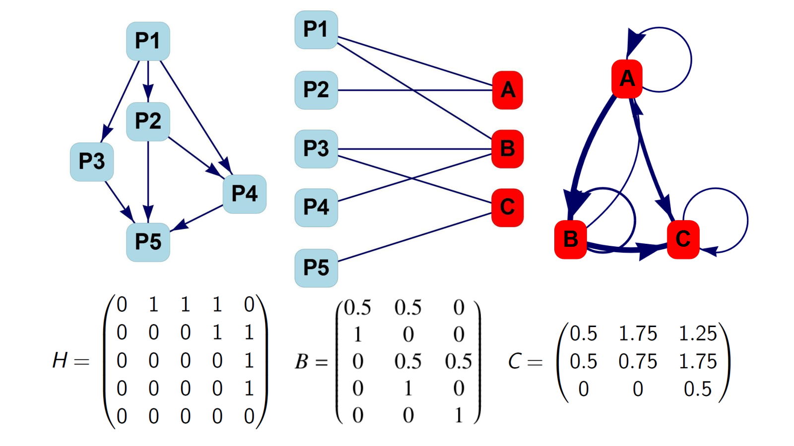
To obtain a temporal representation of knowledge flows, we index the patent citation network by time, $H_{t}$, where the time index refers to the citing patent. The time-indexed bipartite network $B_{t}$ includes all the patents which cite and have been cited at time point $t$, as well as the corresponding technology classes. The time dependent technology citation matrix $C_{t}$ is obtained by applying Eq. (17) to these matrices. The temporal network $W_{t}$ row-normalizes the technology citation matrix as shown in the main text (Eq. 1). The $i^{\text{th}}$ row of $W_{t}$ can be interpreted as the technological reliance of technology $i$ at time $t$ as it contains all the links from patents in $i$ to all other technology classes at the particular time point. The structural stability of the network is investigated further in the supplementary information.

Appendix B Significance sampling

Technology citation networks are prone to be biased due to impinging factors such as the number of patents in a class or the age of patents. Size effects can drive the number of citations between technologies, because the expected number of citations between two technological classes increases with the number of patents in the classes. Another important source of bias is the age of a patent. A new patent might have few forward citations because other inventions simply did not have the time to cite the patent. To eliminate the size and age biases, Alstott et al. (2017) suggest an algorithm to sample random network realizations conditional on domain sizes and patent ages. The algorithm yields networks which preserve these impinging factors, but are random otherwise. The random realizations can then be used to derive a z-score for each link in the network. Links between technological domains which one would expect by chance, will have small z-scores and can be removed.

The randomized controls are generated as follows. First, identify all citations with a specific time lag which have been made in a particular year. An example would be to take all the citations made by patents in the year 2000 which cite patents three years earlier. Then, second, reshuffle all the cited patents. In the example, patents issued in 2000 would point randomly to the set of patents issued three years earlier. Larger classes will receive more citations on average. Note that the total number of citations for a given time lag are preserved by this procedure. By repeating the algorithm many times, an expected number of citations between classes can be derived, as well as the standard deviation. The link expectations and standard deviations are then used to compute the z-scores.

Sampling a large number of random networks for every year between 1947 and 2017 is computationally costly. Therefore, we analytically derive z-scores for every potential inter-domain link as suggested by Alstott et al. (2017) who have shown that the analytical derivation approximates the numerical randomization process very well. The randomization procedure can be stated as drawing from a hypergeometric distribution. Recall that a hypergeometric distribution is the probability of observing a certain number of successes in $n$ draws, without replacement, from a sample of size $s$ containing $k$ objects with the success feature.

In our context, the hypergeometric distribution describes the probability of observing a certain number of citations from class $i$ to class $j$ at $t$ with lag $l$. Let us denote the number of citations between two classes at $t$ and given lag $l$ with $C_{ij,t(t-l)}$. The sample size $s$ is then simply the total number of inter-domain citations, $s_{t(t-l)}=\sum_{i,j}C_{ij,t(t-l)}(1-\delta_{ij})$. The number of draws $n$ corresponds to the number of citations made by a given class $i$. Thus, $n_{i,t-l}=\sum_{j\neq i}C_{ij,t(t-l)}$. The number of successes $k$ is the number of citations received by $j$ at $t-l$, i.e. $k_{j,t-l}=\sum_{i\neq j}C_{ij,t(t-l)}$.

The expected number of patents from $i$ to $j$ at $t$ for all possible lags can then be found by

$$\mathop{\mathbb{E}[C_{ij,t}]}=\sum_{l=0}^{t-1836}\frac{k_{j,t-l}}{s_{t-l}}n_{i,t-l},$$ (18)

and, by assuming independent random variables, the standard deviation is given by

$$\sigma_{ij,t}=\left(\sum_{l=0}^{t-1836}n_{i,t-l}\frac{k_{j,t-l}}{s_{t-l}}\left(1-\frac{k_{j,t-l}}{s_{t-l}}\right)\frac{s_{t-l}-n_{i,t-l}}{s_{t-l}-1}\right)^{1/2}.$$ (19)

For each entry in the citation matrix we calculate z-scores based on

$$z_{ij,t}=\frac{C_{ij,t}-\mathop{\mathbb{E}[C_{ij,t}]}}{\sigma_{ij,t}}.$$ (20)

We eliminate all citations in the technology citation matrix $C_{t}$ with z-score smaller 2, roughly corresponding to the 97.5% quantile of the standard normal distribution. As we show in more detail in the supplementary information, the significance sampling yields substantially sparser networks.

Appendix C Estimation of network model

The econometric network model, Eq. (6), is estimated using maximum likelihood since the OLS estimator is biased and inconsistent due to the reasons outlined in Anselin (2013). The model is related to spatial autoregressive (SAR) models for panel data. But in contrast to most other spatial econometric applications, our model uses a time-varying network term and includes diagonal elements which complicate the estimation. We restate the econometric model in matrix form which will prove useful in the derivation of the estimators.

The model and its corresponding data generating process can be written as

$$g_{t} =V_{t}a+\beta V_{t}\tilde{g}_{t}+\epsilon_{t},\quad t\in\{1,2,...,T\},$$ (21)

$$g_{t} =\left[\mathbb{I}-\beta W_{t}\right]^{-1}a+\left[\mathbb{I}-\beta W_{t}\right]^{-1}\epsilon_{t},$$ (22)

$$\epsilon_{t} \sim N(0,\sigma^{2}\mathbb{I}),$$

where the matrix $V_{t}=V_{t}(\beta)\in\mathbb{R}^{N\times N}$ is diagonal with elements $V_{ii,t}:=(1-\beta W_{ii,t})^{-1}$. $g_{t}$, $a$, $\tilde{g}_{t}$ and $\epsilon_{t}$ are column vectors of length $N$. The $i^{\text{th}}$ element of $\tilde{g}_{t}$ is defined as $\tilde{g}_{i,t}:=\sum_{j=1}^{N}W_{ij,t}g_{j,t}(1-\delta_{ij})$.

The likelihood function is given by

$$\text{LogL}\left((\sigma^{2},a,\beta)|\{g_{t}\}\right)=$$ (23)

$$-\frac{NT}{2}\ln(2\pi\sigma^{2})+\sum_{t=1}^{T}\ln|\mathbb{I}-\beta V_{t}{W}_{t}|-\frac{1}{2\sigma^{2}}\sum_{t=1}^{T}\epsilon_{t}^{\top}\epsilon_{t}.$$

To find the network specific parameter $\beta$, we first optimize the log-likelihood function with respect to $\sigma^{2}$ and $a_{i}$. Following the usual procedure in spatial autoregressive models, we then numerically optimize the concentrated log-likelihood function with respect to $\beta$ (Ord, 1975; Elhorst, 2014; Wang and Yu, 2015). Maximizing the log-likelihood function with respect to $\sigma^{2}$ and $a_{i}$ yields the following expressions:

$$\hat{\sigma}^{2} =\frac{\sum_{t}\epsilon_{t}^{\top}\epsilon_{t}}{NT},$$

$$\hat{a} =\left(\sum_{t}V_{t}^{2}\right)^{-1}\sum_{t}V_{t}g_{t}-\beta\left(\sum_{t}V_{t}^{2}\right)^{-1}\sum_{t}V_{t}^{2}\tilde{g}_{t}.$$

By plugging the found expressions into Eq. (23), we find parameter $\beta$ through the following optimization problem

$$\underset{\beta}{\text{argmax}}\quad constant+\sum_{t=1}^{T}\ln|\mathbb{I}-\beta V_{t}{W}_{t}|-\frac{NT}{2}\ln\sum_{t=1}^{T}\tilde{\epsilon}_{t}^{\top}\tilde{\epsilon}_{t},$$ (24)

with $\tilde{\epsilon}_{t}:=g_{t}-V_{t}\left(\sum_{t}V_{t}^{2}\right)^{-1}\sum_{t}V_{t}g_{t}-\beta V_{t}\left(\sum_{t}V_{t}^{2}\right)^{-1}\sum_{t}V_{t}^{2}\tilde{g}_{t}$. The (asymptotic) variance-covariance matrix is obtained as the Fisher information matrix, i.e. by inverting the numerically computed Hessian of the negative log-likelihood function.

Appendix D Details on predictions

For both the ARIMA and the unconditional network model forecasts we fine-tune the models in-sample to achieve good out-of-sample forecasts of patenting levels. As frequently done in statistical learning, we split the data set into three parts: a training set (1948-1987), a validation set (1988-2002) and a test set (2003-2017). We first calibrate the models to the training set and use different specifications, as outlined below, to predict patenting in every domain in the validation set. We then choose the models which yield the lowest median absolute percentage error in the validation set forecasts. We use median absolute percentage errors over mean absolute percentage errors, since the well-known downward bias of the mean absolute percentage error Armstrong (1985) tends to favor predictors which are systematically underestimating. After choosing the best model specifications, we re-estimate the models to the whole data set up to 2002. Using these parametrizations of the “optimal” models, we then predict patenting activities for every single year and technology from 2003 to 2017.

In case of the ARIMA predictions, a choice has to be made regarding how many MA and AR terms to include in the predictions. Following the proposed principles, we first estimate all possible ARIMA models with lags $\{(p,q)|\;p,q\in\{0,...,5\}\}$ for a given technology in the training set. Second, we use all estimated configurations to predict patenting levels in the validation set. The model specification which reduces the median absolute percentage error in the validation set is then chosen to predict patenting activities in the test set. This procedure is repeated for every single time series.

For the unconditional network model forecasts we follow a similar approach to obtain the optimal order $k^{\prime}$. To see why we optimize the network model with respect to $k^{\prime}$, note that the data generating process in Eq. (22) for given parameters implies $\mathbb{E}[g_{t}]=\left(\mathbb{I}-\beta W_{t}\right)^{-1}a$ and $\mathbb{V}[g_{t}]=\sigma^{2}\left[(\mathbb{I}-\beta W_{t}^{\top})(\mathbb{I}-\beta W_{t})\right]^{-1}$, entailing an exploding variance for $\beta$ approaching one. Since our estimations suggest that $\beta$ is actually close to one, forecast errors are expected to be large. To alleviate this issue, we take advantage of the power series expansion, $\left(\mathbb{I}-\beta W_{t}\right)^{-1}=\sum_{k=0}^{\infty}\beta^{k}W_{t}^{k}$, by defining the predictor as $\hat{g}_{t}^{uncond.}=(\sum_{k=0}^{k^{\prime}}\hat{\beta}^{k}W_{t}^{k})\hat{a}$. Increasing $k^{\prime}$ reduces the bias, versus reducing $k^{\prime}$ lowers the variance. To find the best choice of $k^{\prime}$, we first estimate the model based on the training set and use the defined predictor to forecast patenting activities in the validation set. We then choose $k^{\prime}$ such that the median absolute percentage error, across time and technologies, in the validation set is minimized. The selection procedure yields $k^{\prime}=3$. As discussed in the main text, we found different magnitudes of network dependence for different growth rate lags. We therefore estimated the network model for every growth rate lag (1-year, 2-years, …, 15-years) separately.

This approach assumes that the optimal choice in the validation set also corresponds to the best choice in the test set which does not always have to be the case. The dependence between variables can change over time, an aspect which is not taken into account here. Alternative approaches could be considered in future research. For the conditional forecasts, no further model fine-tuning has to be done.

References

- Acemoglu et al. (2016) Acemoglu D, Akcigit U, Kerr WR. Innovation network. Proceedings of the National Academy of Sciences 2016;113(41):11483–8. doi:10.1073/pnas.1613559113.
- Aghion and Howitt (1990) Aghion P, Howitt P. A model of growth through creative destruction. Technical Report; National Bureau of Economic Research; 1990. doi:10.3386/w3223.
- Alstott et al. (2017) Alstott J, Triulzi G, Yan B, Luo J. Mapping technology space by normalizing patent networks. Scientometrics 2017;110(1):443–79. doi:10.1007/s11192-016-2107-y.
- Anselin (2013) Anselin L. Spatial econometrics: methods and models. volume 4. Springer Science & Business Media, 2013.
- Armstrong (1985) Armstrong JS. Long-Range Forecasting: From Crystal Ball to Computer. volume 2. Wiley, 1985.
- Arthur (2009) Arthur WB. The nature of technology: What it is and how it evolves. Simon and Schuster, 2009.
- Bagley et al. (1992) Bagley RJ, Farmer JD, Fontana W. Evolution of a metabolism. Artificial life II 1992;10:141–58.
- Cowan and Jonard (2003) Cowan R, Jonard N. The dynamics of collective invention. Journal of Economic Behavior & Organization 2003;52(4):513–32. doi:10.1016/S0167-2681(03)00091-X.
- Elhorst (2014) Elhorst JP. Spatial Econometrics: From Cross-Sectional Data to Spatial Panels. volume 479. Springer, 2014.
- Ertur and Koch (2007) Ertur C, Koch W. Growth, technological interdependence and spatial externalities: theory and evidence. Journal of Applied Econometrics 2007;22(6):1033–62. doi:10.1002/jae.963.
- Farmer et al. (1986) Farmer JD, Kauffman SA, Packard NH. Autocatalytic replication of polymers. Physica D: Nonlinear Phenomena 1986;22(1-3):50–67.
- Farmer and Lafond (2016) Farmer JD, Lafond F. How predictable is technological progress? Research Policy 2016;45(3):647–65. doi:10.1016/j.respol.2015.11.001.
- Fink and Reeves (2019) Fink T, Reeves M. How much can we influence the rate of innovation? Science Advances 2019;5(1):eaat6107. doi:10.1126/sciadv.aat6107.
- Fleming (2001) Fleming L. Recombinant uncertainty in technological search. Management Science 2001;47(1):117–32. doi:10.1287/mnsc.47.1.117.10671.
- Grossman and Helpman (1991) Grossman GM, Helpman E. Quality ladders in the theory of growth. The Review of Economic Studies 1991;58(1):43–61. doi:10.2307/2298044.
- Hall et al. (2010) Hall BH, Mairesse J, Mohnen P. Measuring the Returns to R&D. In: Handbook of the Economics of Innovation. Elsevier; volume 2; 2010. p. 1033–82. doi:10.1016/S0169-7218(10)02008-3.
- Ho et al. (2018) Ho CY, Wang W, Yu J. International knowledge spillover through trade: A time-varying spatial panel data approach. Economics Letters 2018;162:30–3. doi:10.1016/j.econlet.2017.10.015.
- Jain and Krishna (2001) Jain S, Krishna S. A model for the emergence of cooperation, interdependence, and structure in evolving networks. Proceedings of the National Academy of Sciences 2001;98(2):543–7. doi:10.1073/pnas.98.2.543.
- Jones (1995) Jones CI. R&D-based models of economic growth. Journal of Political Economy 1995;103(4):759–84. doi:10.1086/262002.
- Kauffman (1993) Kauffman SA. The origins of order: Self-organization and selection in evolution. OUP USA, 1993.
- König et al. (2011) König MD, Battiston S, Napoletano M, Schweitzer F. Recombinant knowledge and the evolution of innovation networks. Journal of Economic Behavior & Organization 2011;79(3):145–64. doi:10.1016/j.jebo.2011.01.007.
- Lafond and Kim (2019) Lafond F, Kim D. Long-run dynamics of the US patent classification system. Journal of Evolutionary Economics 2019;:1–34doi:10.1007/s00191-018-0603-3.
- Leontief (1936) Leontief WW. Quantitative input and output relations in the economic systems of the United States. The Review of Economics and Statistics 1936;:105–25doi:10.2307/1927837.
- Masuda and Lambiotte (2016) Masuda N, Lambiotte R. A Guide to Temporal Networks. World Scientific, 2016.
- McNerney et al. (2011) McNerney J, Farmer JD, Redner S, Trancik JE. Role of design complexity in technology improvement. Proceedings of the National Academy of Sciences 2011;108(22):9008–13. doi:10.1073/pnas.1017298108.
- Miller and Blair (2009) Miller RE, Blair PD. Input-output analysis: foundations and extensions. Cambridge University Press, 2009.
- Napolitano et al. (2018) Napolitano L, Evangelou E, Pugliese E, Zeppini P, Room G. Technology networks: the autocatalytic origins of innovation. Royal Society Open Science 2018;5(6):172445. doi:10.1098/rsos.172445.
- Ord (1975) Ord K. Estimation methods for models of spatial interaction. Journal of the American Statistical Association 1975;70(349):120–6.
- Romer (2012) Romer D. Advanced Macroeconomics. New York: McGraw-Hill, 2012.
- Romer (1990) Romer PM. Endogenous technological change. Journal of Political Economy 1990;98(5/2):71–102. doi:10.1086/261725.
- Schumpeter (1939) Schumpeter JA. Business Cycles. New York: McGraw-Hill Book Company, 1939.
- Taalbi (2018) Taalbi J. Evolution and structure of technological systems-an innovation output network. arXiv preprint arXiv:181106772 2018;.
- Tria et al. (2014) Tria F, Loreto V, Servedio VDP, Strogatz SH. The dynamics of correlated novelties. Scientific Reports 2014;4:5890. doi:10.1038/srep05890.
- Triulzi et al. (2018) Triulzi G, Alstott J, Magee CL. Estimating technology performance improvement rates by mining patent data 2018;doi:10.2139/ssrn.2987588.
- Usher (1954) Usher AP. A History of Mechanical Invention. Cambridge, MA: Harvard University Press, 1954.
- Wang and Yu (2015) Wang W, Yu J. Estimation of spatial panel data models with time varying spatial weights matrices. Economics Letters 2015;128:95–9. doi:10.1016/j.econlet.2015.01.021.
- Youn et al. (2015) Youn H, Strumsky D, Bettencourt LM, Lobo J. Invention as a combinatorial process: evidence from US patents. Journal of The Royal Society Interface 2015;12(106):1–8. doi:10.1098/rsif.2015.0272.