Abstract

Many applications of AI involve scoring individuals using a learned function of their attributes. These predictive risk scores are then used to take decisions based on whether the score exceeds a certain threshold, which may vary depending on the context. The level of delegation granted to such systems in critical applications like credit lending and medical diagnosis will heavily depend on how questions of fairness can be answered. In this paper, we study fairness for the problem of learning scoring functions from binary labeled data, a classic learning task known as bipartite ranking. We argue that the functional nature of the ${\rm ROC}$ curve, the gold standard measure of ranking accuracy in this context, leads to several ways of formulating fairness constraints. We introduce general families of fairness definitions based on the ${\rm AUC}$ and on ${\rm ROC}$ curves, and show that our ${\rm ROC}$-based constraints can be instantiated such that classifiers obtained by thresholding the scoring function satisfy classification fairness for a desired range of thresholds. We establish generalization bounds for scoring functions learned under such constraints, design practical learning algorithms and show the relevance our approach with numerical experiments on real and synthetic data.

1 INTRODUCTION

With the availability of data at ever finer granularity and the development of technological bricks to efficiently store and process this data, the infatuation with machine learning (ML) and artificial intelligence (AI) is spreading to nearly all fields (science, transportation, energy, medicine, security, banking, insurance, commerce…). Expectations are high. There is no denying the opportunities, and we can rightfully hope for an increasing number of successful deployments in the near future. However, AI will keep its promises only if certain issues are addressed. In particular, ML systems that make significant decisions for humans, regarding for instance credit lending in the banking sector (Chen, 2018), diagnosis in medicine (Deo, 2015) or recidivism prediction in criminal justice (Rudin et al., 2018), should guarantee that they do not penalize certain groups of individuals.

Hence, stimulated by the societal expectations, notions of fairness in ML as well guarantees that they can be fulfilled by models trained under appropriate constraints have recently been the subject of a good deal of attention in the literature, see e.g. (Dwork et al., 2012; Kleinberg et al., 2017) among others. Fairness constraints are generally modeled by means of a (qualitative) sensitive variable, indicating membership to a certain group (e.g., ethnicity, gender). The vast majority of the work dedicated to algorithmic fairness in ML focuses on binary classification. In this context, fairness constraints force classifiers to have similar true positive rates (or false positive rates) across sensitive groups. For instance, Hardt et al. (2016); Pleiss et al. (2017) propose to modify a pre-trained classifier in order to fulfill such constraints without deteriorating too much the classification performance. Other work incorporates fairness constraints in the learning stage (Agarwal et al., 2018; Woodworth et al., 2017; Zafar et al., 2017a; Zafar et al., 2017b; Zafar et al., 2019; Menon and Williamson, 2018; Bechavod and Ligett, 2017, see e.g.,). In addition to algorithms, statistical guarantees (in the form of generalization bounds) are crucial for fair ML, as they ensure that the desired fairness constraint will be met at deployment. Such learning guarantees have been established by Donini et al. (2018) for the case of fair classification.

Many real-world problems are however not concerned with learning a binary classifier but rather aim to learn a scoring function. This statistical learning problem is known as bipartite ranking and covers in particular tasks such as credit scoring in banking, pathology scoring in medicine or recidivism scoring in criminal justice, for which fairness is a major concern (Kallus and Zhou, 2019). While it can be formulated in the same probabilistic framework as binary classification, bipartite ranking is not a local learning problem: the goal is not to guess whether a binary label $Y$ is positive or negative from an input observation $X$ but to rank any collection of observations $X_{1},\;\ldots,\;X_{n}$ by means of a scoring function $s:\mathcal{X}\rightarrow\mathbb{R}$ so that observations with positive labels are ranked higher with large probability. Due to the global nature of the task, evaluating the performance is itself a challenge. The gold standard measure, the ${\rm ROC}$ curve, is functional: it is the PP-plot of the false positive rate (FPR) vs the true positive rate (TPR), and the higher the curve, the more accurate the ranking induced by $s$. Sup-norm optimization of the ${\rm ROC}$ curve has been investigated by Clémençon and Vayatis (2009); Clémençon and Vayatis (2010), while most of the literature focuses on the maximization of scalar summaries of the ${\rm ROC}$ curve such as the ${\rm AUC}$ criterion (Agarwal et al., 2005; Clémençon et al., 2008; Zhao et al., 2011) or alternative measures (Rudin, 2006; Clémençon and Vayatis, 2007; Menon and Williamson, 2016).

A key advantage of learning a scoring function over learning a classifier is the flexibility in thresholding the scores so as to obtain false/true positive rates that fit the particular operational constraints in which the decision is taken. A natural fairness requirement in this context is that a fair scoring function should lead to fair decisions for all thresholds of interest. To help fix ideas and grasp the methodological challenge, we describe below a concrete example to motivate our work.

Example 1 (Credit-risk screening).

A bank grants a loan to a client with socio-economic features $X$ if his/her score $s(X)$ is above a certain threshold $t$. As the degree of risk aversion of the bank may vary, the precise deployment threshold $t$ is unknown when choosing the scoring function $s$, although the bank is generally interested in regimes where the probability of default is sufficiently small (low FPR). The bank would like to design a scoring function that ranks higher the clients that are more likely to repay the loan (ranking performance), while ensuring that any threshold in the regime of interest will lead to similar false negative rates across sensitive groups (fairness constraint).

Figure 1: Illustrating the limitations of ${\rm AUC}$-based fairness. Here, the group-wise positive/negative distributions (top) satisfy ${\rm AUC}_{H_{s},G_{s}^{(0)}}={\rm AUC}_{H_{s},G_{s}^{(1)}}$ (bottom left), but yield very different TPR’s at low FPR’s (bottom left). Our new ${\rm ROC}$-based constraints can align scores distributions where it matters, e.g. for low FPR’s as in Example 1 (bottom right).

Contributions. In this work, we provide a thorough study of fairness in bipartite ranking. Our starting point is a number of fairness measures introduced independently in recent papers from different communities (Borkan et al., 2019; Beutel et al., 2019; Kallus and Zhou, 2019). We first show that these are special cases of a general family of fairness constraints based on the ${\rm AUC}$, that we precisely characterize. We then argue that, because it is defined from scalar summaries of functional curves, ${\rm AUC}$-based fairness is oblivious to potentially large disparities between groups at particular locations of the score distribution (see Fig. 1, bottom left). As a consequence, they fail to address use-cases where fairness is needed at specific thresholds (as in Example 1). To overcome these limitations, we introduce a novel functional view of fairness based on ${\rm ROC}$ curves. These richer pointwise ${\rm ROC}$-based constraints can be instantiated to align group-wise score distributions at specific functional points (see Fig. 1, bottom right) and thereby ensure that classifiers obtained by thresholding the scoring function satisfy classification fairness for a certain range of thresholds, as desired in cases like Example 1.

Based on the above, we then introduce empirical risk minimization formulations for learning fair scoring functions under both ${\rm AUC}$ and ${\rm ROC}$-based fairness constraints and establish the first generalization bounds for fair bipartite ranking. Due to the complex nature of the ranking measures, our proof techniques largely differ from the classification results of Donini et al. (2018) as they require non standard technical tools (e.g. to control deviations of ratios of $U$-statistics). In addition to our conceptual contributions and theoretical analysis, we propose efficient training algorithms based on gradient descent and illustrate the practical relevance of our approach on synthetic and real datasets.

Outline. The paper is organized as follows. Section 2 reviews bipartite ranking as well as existing fairness notions for classification and ranking. Section 3 studies ${\rm AUC}$-based fairness constraints and propose richer ${\rm ROC}$-based constraints. In Section 4, we formulate the problem of fair scoring under both ${\rm AUC}$ and ${\rm ROC}$-based fairness constraints and prove statistical learning guarantees. Section 5 presents numerical experiments, and we conclude in Section 6. Due to space limitations, some technical details and additional experiments are postponed to the supplementary.

2 BACKGROUND & RELATED WORK

In this section, we introduce the main concepts involved in the subsequent analysis and review related work. Here and throughout, the indicator function of any event $\mathcal{E}$ is denoted by $\mathbb{I}\{\mathcal{E}\}$ and the pseudo-inverse of any cumulative distribution function (c.d.f.) function $F:\mathbb{R}\to[0,1]$ by $F^{-1}(u)=\inf\left\{t\in\mathbb{R}:F(t)\geq u\right\}$.

2.1 Probabilistic Framework

Let $X$ and $Y$ be two random variables: $Y$ denotes the binary output label (taking values in $\{-1,+1\}$) and $X$ denotes the input features, taking values in a space $\mathcal{X}\subset\mathbb{R}^{d}$ with $d\geq 1$ and modeling some information hopefully useful to predict $Y$. For convenience, we introduce the proportion of positive instances $p:=\mathbb{P}\{Y=+1\}$, as well as $G$ and $H$, the conditional distributions of $X$ given $Y=+1$ and $Y=-1$ respectively. The joint distribution of $(X,Y)$ is fully determined by the triplet $(p,G,H)$. Another way to specify the distribution of $(X,Y)$ is through the pair $(\mu,\eta)$ where $\mu$ denotes the marginal distribution of $X$ and $\eta$ the function $\eta(x):=\mathbb{P}\{Y=+1\mid X=x\}$. With these notations, one may write $\eta(x)=p(dG/dH)(x)/(1-p+p(dG/dH)(x))$ and $\mu=pG+(1-p)H$.

In the context of fairness, we consider a third random variable $Z$ which denotes the sensitive attribute taking values in $\{0,1\}$. The pair $(X,Y)$ is said to belong to salient group $0$ (resp. $1$) when $Z=0$ (resp. $Z=1$). The distribution of the triplet $(X,Y,Z)$ can be expressed as a mixture of the distributions of $X,Y|Z=z$. Following the conventions described above, we introduce the quantities $p_{z},G^{(z)},H^{(z)}$ as well as $\mu^{(z)},\eta^{(z)}$. For instance, $p_{0}=\mathbb{P}\{Y=+1|Z=0\}$ and the distribution of $X|Y=+1,Z=0$ is written $G^{(0)}$, i.e. for $A\subset\mathcal{X}$, $G^{(0)}(A)=\mathbb{P}\{X\in A|Y=+1,Z=0\}$. We denote the probability of belonging to group $z$ by $q_{z}:=\mathbb{P}\{Z=z\}$, with $q_{0}=1-q_{1}$.

2.2 Bipartite Ranking

The goal of bipartite ranking is to learn an order relationship on $\mathcal{X}$ for which positive instances are ranked higher than negative ones with high probability. This order is defined by transporting the natural order on the real line to the feature space through a scoring function $s:\mathcal{X}\to\mathbb{R}$. Given a distribution $F$ over $\mathcal{X}$ and a scoring function $s$, we denote by $F_{s}$ the cumulative distribution function of $s(X)$ when $X$ follows $F$. Specifically:

$$G_{s}(t) :=\mathbb{P}\{s(X)\leq t\mid Y=+1\}=G(s(X)\leq t),$$

$$H_{s}(t) :=\mathbb{P}\{s(X)\leq t\mid Y=-1\}=H(s(X)\leq t).$$

ROC analysis. ROC curves are widely used to visualize the dissimilarity between two real-valued distributions in many applications, e.g. anomaly detection, medical diagnosis, information retrieval.

Definition 1 (ROC curve).

Let $g$ and $h$ be two cumulative distribution functions on $\mathbb{R}$. The ${\rm ROC}$ curve related to $g$ and $h$ is the graph of the mapping:

$${\rm ROC}_{h,g}:\alpha\in[0,1]\mapsto 1-g\circ h^{-1}(1-\alpha).$$

When $g$ and $h$ are continuous, it can alternatively be defined as the parametric curve $t\in\mathbb{R}\mapsto(1-h(t),1-g(t))$.

The classic area under the ${\rm ROC}$ curve (${\rm AUC}$) criterion is a scalar summary of the functional measure of dissimilarity ${\rm ROC}$. Formally, we have:

$${\rm AUC}_{h,g} :=\int{\rm ROC}_{h,g}(\alpha)d\alpha=\mathbb{P}\{S>S^{\prime}\}+\frac{1}{2}\mathbb{P}\{S=S^{\prime}\},$$

where $S$ and $S^{\prime}$ denote independent random variables, whose c.d.f.’s are $h$ and $g$ respectively.

In bipartite ranking, one focuses on the ability of the scoring function $s$ to separate positive from negative data. This is reflected by ${\rm ROC}_{H_{s},G_{s}}$, which gives the false positive rate vs. true positive rate of binary classifiers $g_{s,t}:x\mapsto 2\cdot\mathbb{I}\{s(x)>t\}-1$ obtained by thresholding $s$ at all possible thresholds $t\in\mathbb{R}$. The global summary ${\rm AUC}_{H_{s},G_{s}}$ serves as a standard performance measure (Clémençon et al., 2008).

Empirical estimates. In practice, the scoring function $s$ is learned based on a training set $\{(X_{i},Y_{i})\}_{i=1}^{n}$ of $n$ i.i.d. copies of the random pair $(X,Y)$. Let $n_{+}$ and $n_{-}$ be the number of positive and negative data points respectively. We introduce $\widehat{G}_{s}$ and $\widehat{H}_{s}$, the empirical counterparts of $G_{s}$ and $H_{s}$:

$$\widehat{G}_{s}(t) :=(1/n_{+})\textstyle\sum_{i=1}^{n}\mathbb{I}\{Y_{i}=+1,s(X_{i})\leq t\},$$

$$\widehat{H}_{s}(t) :=(1/n_{-})\textstyle\sum_{i=1}^{n}\mathbb{I}\{Y_{i}=-1,s(X_{i})\leq t\}.$$

Note that the denominators $n_{+}$ and $n_{-}$ are sums of i.i.d. random (indicator) variables. For any two distributions $F,F^{\prime}$ over $\mathbb{R}$, we denote the empirical counterparts of ${\rm AUC}_{F,F^{\prime}}$ and ${\rm ROC}_{F,F^{\prime}}$ by $\widehat{{\rm AUC}}_{F,F^{\prime}}:={\rm AUC}_{\widehat{F},\widehat{F^{\prime}}}$ and $\widehat{{\rm ROC}}_{F,F^{\prime}}(\cdot):={\rm ROC}_{\widehat{F},\widehat{F^{\prime}}}(\cdot)$ respectively. In particular, we have:

$$\widehat{{\rm AUC}}_{H_{s},G_{s}}:= ~\textstyle\frac{1}{n_{+}n_{-}}\sum_{i<j}K((s(X_{i}),Y_{i}),(s(X_{j}),Y_{j})),$$

where $K((t,y),(t^{\prime},y^{\prime}))=\mathbb{I}\{(y-y^{\prime})(t-t^{\prime})>0\}+\mathbb{I}\{y\neq y^{\prime},t=t^{\prime}\}/2$ for any $t,t^{\prime}\in\mathbb{R}^{2},y,y^{\prime}\in\{-1,+1\}^{2}$. Empirical risk minimization for bipartite ranking typically consists in maximizing $\widehat{{\rm AUC}}_{H_{s},G_{s}}$ over a class of scoring functions (Clémençon et al., 2008; Zhao et al., 2011, see e.g.).

2.3 Fairness in Binary Classification

In binary classification, the goal is to learn a mapping function $g:\mathcal{X}\mapsto\{-1,+1\}$ that predicts the output label $Y$ from the input random variable $X$ as accurately as possible (as measured by an appropriate loss function). Any classifier $g$ can be defined by its unique acceptance set $A_{g}:=\{x\in\mathcal{X}\mid g(x)=+1\}\subset\mathcal{X}$.

Existing notions of fairness for binary classification (see Zafar et al., 2019, for a detailed treatment) aim to ensure that $g$ makes similar predictions (or errors) for the two groups. We mention here the common fairness definitions that depend on the ground truth label $Y$. Parity in mistreatment requires that the proportion of errors is the same for the two groups:

$$M^{(0)}(g)=M^{(1)}(g),$$ (1)

where $M^{(z)}(g):=\mathbb{P}\{g(X)\neq Y\mid Z=z\}$. While this requirement is natural, it considers that all errors are equal: in particular, one can have a high false positive rate (FPR) $H^{(1)}(A_{g})$ for one group and a high false negative rate (FNR) $G^{(0)}(A_{g})$ for the other. This can be considered unfair when acceptance is an advantage, e.g. being granted a loan in Example 1). A solution is to consider parity in false positive rates and/or parity in false negative rates, which respectively write:

$$H^{(0)}(A_{g})=H^{(1)}(A_{g})\text{ and }G^{(0)}(A_{g})=G^{(1)}(A_{g}).$$ (2)

Remark 1 (Connection to bipartite ranking).

A score function $s:\mathcal{X}\to\mathbb{R}$ induces an infinite collection of binary classifiers $g_{s,t}:x\mapsto 2\cdot\mathbb{I}\{s(x)>t\}-1$. While one could fix a threshold $t\in\mathbb{R}$ in advance and enforce fairness on $g_{s,t}$, we are interested here in notions of fairness for the score function itself (see Example 1).

2.4 Fairness in Ranking

Fairness for rankings has been mostly considered in the informational retrieval and recommender systems communities. Given a set of items with known relevance scores, they aim to extract a (partial) ranking that balances utility and notions of fairness at the group or individual level, or through a notion of exposure over several queries (Zehlike et al., 2017; Celis et al., 2018; Biega et al., 2018; Singh and Joachims, 2018). Singh and Joachims (2019) and Beutel et al. (2019) extend the above work to the learning to rank framework, where the task is to learn relevance scores and ranking policies from a certain number of observed queries that consist of query-item features and item relevance scores. This is fundamentally different from the bipartite ranking setting considered here.

AUC constraints. In a setting closer to ours, Kallus and Zhou (2019) introduce measures to quantify the fairness of a known scoring function on binary labeled data (they do not address learning). Their approach is based on the ${\rm AUC}$, which can be seen as a measure of homogeneity between distributions (Clémençon et al., 2009). Similar definitions of fairness are also considered in (Beutel et al., 2019; Borkan et al., 2019).

Introduce $G_{s}^{(z)}$ (resp. $H_{s}^{(z)}$) as the c.d.f. of the score on the positives (resp. negatives) of group $z\in\{0,1\}$, i.e. $G_{s}^{(z)}(t)=G^{(z)}(s(X)\leq t)$ and $H_{s}^{(z)}(t)=H^{(z)}(s(X)\leq t)$, for any $t\in\mathbb{R}$. Precise examples of ${\rm AUC}$-based fairness constraints include: 1) the intra-group pairwise ${\rm AUC}$ fairness (Beutel et al., 2019),

$${\rm AUC}_{H_{s}^{(0)},G_{s}^{(0)}}={\rm AUC}_{H_{s}^{(1)},G_{s}^{(1)}},$$ (3)

which requires the ranking performance to be equal within groups, 2) the Background Negative Subgroup Positive (BNSP) ${\rm AUC}$ fairness (Borkan et al., 2019),

$${\rm AUC}_{H_{s},G^{(0)}_{s}} ={\rm AUC}_{H_{s},G^{(1)}_{s}},$$ (4)

which enforces that positive instances from either group have the same probability of being ranked higher than a negative example, 3) the inter-group pairwise ${\rm AUC}$ fairness (Kallus and Zhou, 2019),

$${\rm AUC}_{H_{s}^{(0)},G_{s}^{(1)}}={\rm AUC}_{H_{s}^{(1)},G_{s}^{(0)}},$$ (5)

which imposes that the positives of a group can be distinguished from the negatives of the other group as effectively for both groups. Many more ${\rm AUC}$-based fairness constraints are possible: we give examples (some of them novel) in the supplementary material.

3 FROM AUC TO ROC-BASED FAIRNESS CONSTRAINTS

In this section, we first provide a new general framework to characterize all relevant ${\rm AUC}$ constraints. We then highlight some limitations of ${\rm AUC}$ fairness constraints, which serve as motivation to introduce our richer pointwise ROC-based fairness constraints.

3.1 A Family of AUC Fairness Constraints

All proposed ${\rm AUC}$-based fairness constraints in the literature follow a common structure, which we precisely characterize.

Denote by $(e_{1},e_{2},e_{3},e_{4})$ the canonical basis of $\mathbb{R}^{4}$, as well as by $\mathbf{1}$ the constant vector $\mathbf{1}=\sum_{k=1}^{4}e_{k}$. ${\rm AUC}$ constraints are expressed in the form of equalities of the ${\rm AUC}$’s between mixtures of the c.d.f.’s $D(s)$, with: $D(s):=(H^{(0)}_{s},H^{(1)}_{s},G^{(0)}_{s},G^{(1)}_{s})^{\top}$. Formally, introducing the probability vectors $\alpha,\beta,\alpha^{\prime},\beta^{\prime}\in\mathcal{P}$ where $\mathcal{P}=\{v\mid v\in\mathbb{R}_{+}^{4},\mathbf{1}^{\top}v=1\}$, they write as:

$${\rm AUC}_{\alpha^{\top}D(s),\beta^{\top}D(s)}={\rm AUC}_{\alpha^{\prime\top}D(s),\beta^{\prime\top}D(s)}.$$ (6)

However, observe that Eq. 6 is under-specified in the sense that it includes constraints that actually give an advantage to one of the groups.

We thus introduce a general framework to formulate all relevant AUC-based constraints (and only those) as a linear combination of 5 elementary constraints. Given a scoring function $s$, let the vector $C(s)=(C_{1}(s),\dots,C_{5}(s))^{\top}$ where the $C_{l}(s)$’s are elementary fairness measurements. Specifically, the value of $|C_{1}(s)|$ (resp. $|C_{2}(s)|$) quantifies the resemblance of the distribution of the negatives (resp. positives) between the two sensitive attributes:

$$C_{1}(s) ={\rm AUC}_{H^{(0)}_{s},H^{(1)}_{s}}-1/2,$$

$$C_{2}(s) =1/2-{\rm AUC}_{G^{(0)}_{s},G^{(1)}_{s}},$$

while $C_{3}(s)$, $C_{4}(s)$ and $C_{5}(s)$ measure the difference in ability of a score to discriminate between positives and negatives for any two pairs of sensitive attributes:

$$C_{3}(s) ={\rm AUC}_{H^{(0)}_{s},G^{(0)}_{s}}-{\rm AUC}_{H^{(0)}_{s},G^{(1)}_{s}},$$

$$C_{4}(s) ={\rm AUC}_{H^{(0)}_{s},G^{(1)}_{s}}-{\rm AUC}_{H^{(1)}_{s},G^{(0)}_{s}},$$

$$C_{5}(s) ={\rm AUC}_{H^{(1)}_{s},G^{(0)}_{s}}-{\rm AUC}_{H^{(1)}_{s},G^{(1)}_{s}}.$$

The family of fairness constraints we consider is then the set of linear combinations of the $C_{l}(s)=0$:

$$\mathcal{C}_{\Gamma}(s):\quad\Gamma^{\top}C(s) =\textstyle\sum_{l=1}^{5}\Gamma_{l}C_{l}(s)=0,$$ (7)

where $\Gamma=(\Gamma_{1},\dots,\Gamma_{5})^{\top}\in\mathbb{R}^{5}$.

Theorem 1.

The following statements are equivalent:

1. Eq. 6 is satisfied for any measurable scoring function $s$ when $H^{(0)}=H^{(1)}$, $G^{(0)}=G^{(1)}$ and $\mu(\eta(X)=p)<1$,

2. Eq. 6 is equivalent to $\mathcal{C}_{\Gamma}(s)$ for some $\Gamma\in\mathbb{R}^{5}$,

3. $(e_{1}+e_{2})^{\top}[(\alpha-\alpha^{\prime})-(\beta-\beta^{\prime})]=0$.

Theorem 1 shows that our general family defined by Eq. 7 compactly captures all relevant AUC-based fairness constraints (Beutel et al., 2019; Borkan et al., 2019; Kallus and Zhou, 2019, including those proposed by) while ruling out the ones that are not satisfied when $H^{(0)}=H^{(1)}$ and $G^{(0)}=G^{(1)}$ (which are in fact unfairness constraints). Their parameters $\Gamma$ are provided in Table 1. We refer to the supplementary for the proof of this result and examples of novel fairness constraints that can be expressed with Eq. 7.

Table 1: Value of $\Gamma$ in our formulation of Eq. 7 for AUC-based constraints introduced in previous work.

${\rm AUC}$-based fairness constraint	$\Gamma_{1}$	$\Gamma_{2}$	$\Gamma_{3}$	$\Gamma_{4}$	$\Gamma_{5}$
Intra-group pairwise (Beutel et al., 2019), subgroup ${\rm AUC}$ (Borkan et al., 2019)	$0$	$0$	$\frac{1}{3}$	$\frac{1}{3}$	$\frac{1}{3}$
BNSP ${\rm AUC}$ (Borkan et al., 2019), pairwise accuracy (Beutel et al., 2019)	$0$	$0$	$\frac{q_{0}(1-p_{0})}{1-p}$	$0$	$\frac{q_{1}(1-p_{1})}{1-p}$
BPSN ${\rm AUC}$ (Borkan et al., 2019; Beutel et al., 2019; Kallus and Zhou, 2019)	$0$	$0$	$\frac{q_{0}p_{0}}{2p}$	$\frac{1}{2}$	$\frac{q_{1}p_{1}}{2p}$
Zero Average Equality Gap (Borkan et al., 2019)	$0$	$1$	$0$	$0$	$0$
Inter-group pairwise (Beutel et al., 2019), x${\rm AUC}$ (Kallus and Zhou, 2019)	$0$	$0$	$0$	$1$	$0$

As we show in Section 4.1, our unifying framework enables the design of general formulations and statistical guarantees for learning fair scoring functions, which can then be instantiated to the specific notion of AUC-based fairness that the practitioner is interested in.

3.2 Limitations of AUC-based Constraints

To illustrate the fundamental limitations of ${\rm AUC}$-based fairness constraints, we will rely on the credit-risk screening use case described in Example 1. Imagine that the scoring function $s$ gives the c.d.f.’s $H_{s}^{(z)}$ and $G_{s}^{(z)}$ shown in Fig. 1 (top). Looking at $G_{s}^{(1)}$, we can see that creditworthy ($Y=+1$) individuals of the sensitive group $Z=1$ do not have scores smaller than $0.5$ and have an almost constant positive density of scores between 0.6 and 1. On the other hand, the scores of creditworthy individuals of group $Z=0$ are sometimes low but are mostly concentrated around $1$ (greater than 0.80), as seen from $G_{s}^{(0)}$. The distribution of scores for individuals who do not repay their loan ($Y=-1$) is the same across groups.

Even though the c.d.f.’s $G_{s}^{(0)}$ and $G_{s}^{(1)}$ are very different, the scoring function $s$ satisfies the ${\rm AUC}$ constraint in Eq. 4, as can be seen from Fig. 1 (bottom left). This means that creditworthy individuals from either group have the same probability of being ranked higher than a “bad borrower”. However, using high thresholds (which correspond to low probabilities of default on the granted loans) will lead to unfair decisions for one group. For instance, using $t=0.85$ gives a FNR of 30% for group 0 and of 60% for group $1$, as can be seen from Fig. 1 (top). If the proportion of creditworthy people is the same in each group ($p_{0}q_{0}=p_{1}q_{1}$), we would reject twice as much creditworthy people of group $1$ than of group $0$! This is blatantly unfair in the sense of parity in FNR defined in Eq. 2.

In general, fairness constraints defined by the equality between two ${\rm AUC}$’s only quantify a stochastic order between distributions, not the equality between these distributions. In fact, for continuous ${\rm ROC}$s, the equality between their two ${\rm AUC}$’s only implies that the two ${\rm ROC}$’s intersect at some unknown point. As a consequence, ${\rm AUC}$-based fairness can only guarantee that there exists some threshold $t\in\mathbb{R}$ that induces a non-trivial classifier $g_{s,t}:x\mapsto 2\cdot\mathbb{I}\{s(x)>t\}-1$ satisfying a notion of fairness for classification (see the supplementary for details). Unfortunately, the value of $t$ and the corresponding FPR of the ROC curves are not known in advance and are difficult to control. For the distributions of Fig. 1, we see that the classifier $g_{s,t}$ is fair in FNR only for $t=0.72$ (20% FNR for each group) but has a rather high FPR (i.e., probability of default) of $\sim$25%, which may be not sustainable for the bank.

3.3 Learning with Pointwise ROC-based Fairness Constraints

To impose richer and more targeted fairness conditions, we propose to use pointwise ${\rm ROC}$-based fairness constraints as an alternative to ${\rm AUC}$-based constraints. We start from the “ideal fairness goal” of enforcing the equality of the score distributions of the positives (resp. negatives) between the two groups, i.e. $G_{s}^{(0)}=G_{s}^{(1)}$ (resp. $H_{s}^{(0)}=H_{s}^{(1)}$). This strong functional criterion can be expressed in terms of ROC curves. For $\alpha\in[0,1]$, consider the deviations between the positive (resp. negative) inter-group ROCs and the identity function:

$$\Delta_{G,\alpha}(s) :={\rm ROC}_{G^{(0)}_{s},G^{(1)}_{s}}(\alpha)-\alpha,$$

$$\big(\text{resp. }\Delta_{H,\alpha}(s) :={\rm ROC}_{H^{(0)}_{s},H^{(1)}_{s}}(\alpha)-\alpha\big).$$

The aforementioned condition of equality between the distribution of the positives (resp. negatives) of the two groups are equivalent to satisfying $\Delta_{G,\alpha}(s)=0$ (resp. $\Delta_{H,\alpha}(s)=0$) for any $\alpha\in[0,1]$. When both of those conditions are satisfied, all of the AUC-based fairness constraints covered by Eq. 7 are verified, as it is easy to see that $C_{l}(s)=0$ for all $l\in\{1,\dots,5\}$. Furthermore, guarantees on the fairness of classifiers $g_{s,t}$ induced by $s$ hold for all possible thresholds $t$. While this strong property is in principle desirable, it puts overly restrictive constraints on $s$ that will often completely jeopardize its ranking performance.

We thus propose a general approach to implement the satisfaction of a finite number of fairness constraints on $\Delta_{H,\alpha}(s)$ and $\Delta_{G,\alpha}(s)$ for specific values of $\alpha$ that are relevant to the use case at hand. Our criterion is flexible enough to address the limitations of ${\rm AUC}$-based constraints outlined above. Specifically, a practitioner can choose points for $\Delta_{H,\alpha}$ and $\Delta_{G,\alpha}$ to guarantee the fairness of classifiers obtained by thresholding the scoring function at the desired trade-offs between, say, FPR and FNR. Furthermore, we show in Proposition 1 below (proof in supplementary) that under some regularity assumption on the ${\rm ROC}$ curve (Assumption 1), if a small number of fairness constraints $m_{F}$ are satisfied at discrete points $\alpha_{F}^{(1)},\dots,\alpha_{F}^{(m_{F})}$ of an interval for $F\in\{H,G\}$, then one obtains guarantees in sup norm on $\alpha\mapsto\Delta_{F,\alpha}$ (and therefore fair classifiers) in the entire interval $[\alpha_{F}^{(1)},\alpha_{F}^{(m_{F})}]$. This result is crucial in applications where the threshold used at deployment can vary in a whole interval, such as biometric verification (Grother and Ngan, 2019) and credit-risk screening (see Example 1).

Assumption 1.

The class $\mathcal{S}$ of scoring functions take values in $(0,T)$ for some $T>0$, and the family of cdfs $\mathcal{K}=\{G_{s}^{(z)},H_{s}^{(z)}:s\in\mathcal{S},z\in\{0,1\}\}$ satisfies: (a) any $K\in\mathcal{K}$ is continuously differentiable, and (b) there exists $b,B>0$ s.t. $\forall(K,t)\in\mathcal{K}\times(0,T)$, $b\leq\left\lvert K^{\prime}(t)\right\rvert\leq B$. The latter condition is satisfied when scoring functions do not have flat or steep parts, see Clémençon and Vayatis (2007) (Remark 7) for a discussion.

Proposition 1.

Under Assumption 1, if $\exists F\in\{H,G\}$ s.t. for every $k\in\{1,\dots,m_{F}\}$, $|\Delta_{F,\alpha_{F}^{(k)}}(s)|\leq\epsilon$, then:

$$\sup_{\alpha\in[0,1]}\big|\Delta_{F,\alpha}(s)\big|\leq\epsilon+\frac{B+b}{2b}\max_{k\in\{0,\dots,m\}}\big|\alpha_{F}^{(k+1)}-\alpha_{F}^{(k)}\big|,$$

with the convention $\alpha_{F}^{(0)}=0$ and $\alpha_{F}^{(m_{F}+1)}=1$.

To illustrate how ${\rm ROC}$-based fairness constraints can be designed in a practical case, we return to our credit lending example. In Fig. 1 (bottom right), we have $\Delta_{H,\alpha}(s)=0$ for any $\alpha\in[0,1]$ since $H_{s}^{(0)}=H_{s}^{(1)}$. However, $\Delta_{G,\alpha}(s)$ can be large: this is the case in particular for small $\alpha$’s (low FPR). If the goal is to obtain fair classifiers in FNR for high thresholds (i.e., low FPR), we should seek a scoring function $s$ with $\Delta_{G,\alpha}\simeq 0$ for any $\alpha\leq\alpha_{\text{max}}$, where $\alpha_{\text{max}}$ is the maximum TPR the bank will operate at (see Fig. 1, bottom right). The value of $\alpha_{\text{max}}$ can be chosen based on the performance of a score learned without fairness constraint if the bank seeks to limit FPR’s or maximize its potential earnings. Learning with constraints for $\alpha$’s in an evenly spaced grid on $[0,\alpha_{\text{max}}]$ will ensure that the resulting $s$ yields fair classifiers $g_{s,t}$ for high thresholds $t$, as confirmed experimentally in Section 5.

4 LEARNING UNDER AUC AND ROC FAIRNESS CONSTRAINTS

In this section, we first introduce empirical risk minimization problems for learning under the ${\rm AUC}$ and ${\rm ROC}$-based constraints introduced in Section 3. Then, we prove statistical learning guarantees in the form of generalization bounds, which fill a gap in the existing literature for ${\rm AUC}$-based constraints and provide a theoretical justification for our novel ${\rm ROC}$-based constraints. Finally, we briefly describe how to empirically minimize such criteria with gradient-based algorithms.

4.1 Learning with AUC-based Constraints

We first formulate the problem of bipartite ranking under ${\rm AUC}$-based fairness constraints. Introducing fairness as a hard constraint is tempting, but may be costly in terms of ranking performance. In general, there is indeed a trade-off between the ranking performance and the level of fairness. For a family of scoring functions $\mathcal{S}$ and some instantiation $\Gamma$ of our general fairness definition in Eq. 7, we thus define the learning problem as follows:

$$\textstyle\max_{s\in\mathcal{S}}\quad{\rm AUC}_{H_{s},G_{s}}-\lambda\left\lvert\Gamma^{\top}C(s)\right\rvert,$$ (8)

where $\lambda\geq 0$ is a hyperparameter balancing ranking performance and fairness.

For the sake of simplicity and concreteness, in the rest of this section we focus on a special case of Eq. 8, namely when $C(s)$ corresponds to the fairness definition in Eq. 3. One can easily extend our analysis to any other instance of our general definition in Eq. 7. We denote by $s_{\lambda}^{*}$ the scoring function that maximizes the objective $L_{\lambda}(s)$ of Eq. 8, where:

$$L_{\lambda}(s):={\rm AUC}_{H_{s},G_{s}}-\lambda\big|{\rm AUC}_{H^{(0)}_{s},G^{(0)}_{s}}-{\rm AUC}_{H^{(1)}_{s},G^{(1)}_{s}}\big|.$$

Given a training set $\{(X_{i},Y_{i},Z_{i})\}_{i=1}^{n}$ of $n$ i.i.d. copies of the random triplet $(X,Y,Z)$, we denote by $n^{(z)}$ the number of points in group $z\in\{0,1\}$, and by $n_{+}^{(z)}$ (resp. $n_{-}^{(z)}$) the number of positive (resp. negative) points in $z$. The empirical counterparts of $H^{(z)}_{s}$ and $G^{(z)}_{s}$ are:

$$\widehat{H}_{s}^{(z)}(t) =(1/n_{-}^{(z)})\textstyle\sum_{i=1}^{n}\mathbb{I}\left\{Z_{i}=z,Y_{i}=-1,s(X_{i})\leq t\right\},$$

$$\widehat{G}_{s}^{(z)}(t) =(1/n_{+}^{(z)})\textstyle\sum_{i=1}^{n}\mathbb{I}\left\{Z_{i}=z,Y_{i}=+1,s(X_{i})\leq t\right\}.$$

Recalling the notation $\widehat{{\rm AUC}}_{F,F^{\prime}}:={\rm AUC}_{\widehat{F},\widehat{F}^{\prime}}$ from Section 2.2, the empirical problem writes:

$$\widehat{L}_{\lambda}(s):=\widehat{{\rm AUC}}_{H_{s},G_{s}} -\lambda\big|\widehat{{\rm AUC}}_{H^{(0)}_{s},G^{(0)}_{s}}-\widehat{{\rm AUC}}_{H^{(1)}_{s},G^{(1)}_{s}}\big|.$$

We denote its maximizer by $\widehat{s}_{\lambda}$. We can now state our statistical learning guarantees for fair ranking.

Theorem 2.

Assume the class of functions $\mathcal{S}$ is VC-major with finite VC-dimension $V<+\infty$ and that there exists $\epsilon>0$ s.t. $\min_{z\in\{0,1\},y\in\{-1,1\}}\mathbb{P}\{Y=y,Z=z\}\geq\epsilon$. Then, for any $\delta>0$, for all $n>1$, we have w.p. at least $1-\delta$:

$$\epsilon^{2} \cdot\left[L_{\lambda}(s_{\lambda}^{*})-L_{\lambda}(\widehat{s}_{\lambda})\right]\leq\;C\sqrt{V/n}\cdot\left(4\lambda+1/2\right)$$

$$\qquad+\sqrt{\frac{\log(13/\delta)}{n-1}}\cdot\Big(4\lambda+(4\lambda+2)\epsilon\Big)+O(n^{-1}).$$

Theorem 2 establishes a learning rate of $O(1/\sqrt{n})$ for our problem of ranking under AUC-based fairness constraints, which holds for any distribution of $(X,Y,Z)$ as long as the probability of observing each combination of label and group is bounded away from zero. As the natural estimate of the ${\rm AUC}$ involves sums of dependent random variables, the proof of Theorem 2 does not follow from usual concentration inequalities on standard averages. Indeed, it requires controlling the uniform deviation of ratios of $U$-processes indexed by a class of functions of controlled complexity.

4.2 Learning with ROC-based Constraints

We now turn to the problem of bipartite ranking under ${\rm ROC}$-based fairness constraints. Recall from Section 3.3 that we aim to satisfy some constraints on $\Delta_{H,\alpha}(s)$ and $\Delta_{G,\alpha}(s)$ for specific values of $\alpha$. Denote by $m_{H},m_{G}\in\mathbb{N}$ be the number of constraints for the negatives and the positives respectively, as well as $\alpha_{H}=[\alpha_{H}^{(1)},\dots,\alpha_{H}^{(m_{H})}]\in[0,1]^{m_{H}}$ and $\alpha_{G}=[\alpha_{G}^{(1)},\dots,\alpha_{G}^{(m_{G})}]\in[0,1]^{m_{G}}$ the points at which they apply (sorted in strictly increasing order).

With the notation $\Lambda:=(\alpha,\lambda_{H},\lambda_{G})$, we can introduce the learning objective $L_{\Lambda}(s)$ defined as:

$${\rm AUC}_{H_{s},G_{s}} -\sum_{k=1}^{m_{H}}\lambda_{H}^{(k)}\big|\Delta_{H,\alpha_{H}^{(k)}}(s)\big|-\sum_{k=1}^{m_{G}}\lambda_{G}^{(k)}\big|\Delta_{G,\alpha_{G}^{(k)}}(s)\big|,$$

where $\lambda_{H}=[\lambda_{H}^{(1)},\dots,\lambda_{H}^{(m_{H})}]\in\mathbb{R}_{+}^{m_{H}}$ and $\lambda_{G}=[\lambda_{G}^{(1)},\dots,\lambda_{G}^{(m_{G})}]\in\mathbb{R}_{+}^{m_{G}}$ are hyperparameters.

The empirical counterpart $\widehat{L}_{\Lambda}(s)$ of $L_{\Lambda}$ is defined as:

$$\widehat{{\rm AUC}}_{H_{s},G_{s}}-\sum_{k=1}^{m_{H}}\lambda_{H}^{(k)}\big|\widehat{\Delta}_{H,\alpha_{H}^{(k)}}(s)\big|-\sum_{k=1}^{m_{G}}\lambda_{G}^{(k)}\big|\widehat{\Delta}_{G,\alpha_{G}^{(k)}}(s)\big|,$$

where $\widehat{\Delta}_{H,\alpha}(s)=\widehat{{\rm ROC}}_{G^{(0)}_{s},G^{(1)}_{s}}(\alpha)-\alpha$ and $\widehat{\Delta}_{G,\alpha}(s)=\widehat{{\rm ROC}}_{H^{(0)}_{s},H^{(1)}_{s}}(\alpha)-\alpha$ for any $\alpha\in[0,1]$.

We now prove statistical guarantees for the maximization of $\widehat{L}_{\Lambda}(s)$. We denote by $s_{\Lambda}^{*}$ the maximizer of $L_{\Lambda}$ over $\mathcal{S}$, and by $\hat{s}_{\Lambda}$ the maximizer of $\widehat{L}_{\Lambda}$ over $\mathcal{S}$. Our analysis relies on the regularity assumption on the ${\rm ROC}$ curve provided in Section 3.3 (Assumption 1).

Theorem 3.

Under Assumption 1 and those of Theorem 2, for any $\delta>0$, $n>1$, w.p. $\geq 1-\delta$:

$$\epsilon^{2}\cdot\left[L_{\Lambda}(s_{\Lambda}^{*})-L_{\Lambda}(\widehat{s}_{\Lambda})\right]\leq C\left(1/2+2\epsilon C_{\Lambda,\mathcal{K}}\right)\sqrt{V/n}$$

$$\qquad\qquad\qquad+2\epsilon\left(1+3C_{\Lambda,\mathcal{K}}\right)\sqrt{\frac{\log(19/\delta)}{n-1}}+O(n^{-1}),$$

where $C_{\Lambda,\mathcal{K}}=(1+B/b)(\bar{\lambda}_{H}+\bar{\lambda}_{G})$, with $\bar{\lambda}_{H}=\sum_{k=1}^{m_{H}}\lambda_{H}^{(k)}$ and $\bar{\lambda}_{G}=\sum_{k=1}^{m_{G}}\lambda_{G}^{(k)}$.

Theorem 3 generalizes the learning rate of $O(1/\sqrt{n})$ of Theorem 2 to ranking under ${\rm ROC}$-based constraints. Its proof also relies on results for $U$-processes, but further requires a study of the deviations of the empirical ${\rm ROC}$ curve seen as ratios of empirical processes indexed by $\mathcal{S}\times[0,1]$. In that regard, our analysis builds upon the decomposition proposed in Hsieh and Turnbull (1996), which enables the derivation of uniform bounds over $\mathcal{S}\times[0,1]$ from results on standard empirical processes (van der Vaart and Wellner, 1996).

4.3 Algorithmic Details

In practice, maximizing $\widehat{L}_{\lambda}$ or $\widehat{L}_{\Lambda}$ directly by gradient ascent is not feasible since the criteria are not continuous. We use classic smooth surrogate relaxations of the AUCs or ${\rm ROC}$s based on the logistic function $\sigma:x\mapsto 1/(1+e^{-x})$. We also remove the absolute values in $\widehat{L}_{\lambda}$ and $\widehat{L}_{\Lambda}$, and instead rely on parameters that are modified adaptively during the training process. We solve the problem using a stochastic gradient ascent algorithm, and modify the introduced parameters every fixed number of iterations based on fairness statistics evaluated on a small validation set. We refer to the supplementary material for more details on the algorithms we use in our experiments.

The hyperparameter $\lambda$ should be tuned to achieve the desired trade-off between ranking performance and fairness. For learning under a ${\rm ROC}$-based constraint, Fig. 2 provides examples of trade-offs for different $\lambda$’s on the dataset Adult presented in Section 5.

5 EXPERIMENTS

In this section, we present a subset of our experimental results, which we think nicely illustrates the differences between ${\rm AUC}$ and ${\rm ROC}$-based fairness. It also shows how these constraints can be used to achieve a trade-off between ranking performance and the desired notion of fairness in practical use cases. Due to space limitations, we refer to the supplementary material for the presentation of all details on the experimental setup, as well as additional results.

Figure 2: Ranking accuracy (${\rm AUC}$) and a ${\rm ROC}$-based constraint at $\Delta_{H}(1/8)$ as a function of the hyperparameter $\lambda$, on the Adult dataset.

Figure 3: ${\rm ROC}$ curves on the test set of Adult and Compas for a score learned without and with fairness constraints. Black curves represent ${\rm ROC}_{H_{s},G_{s}}$. We also report the corresponding ranking performance ${\rm AUC}_{H_{s},G_{s}}$.

Results are summarized in Fig. 3, which shows ${\rm ROC}$ curves for 2-layer neural scoring functions learned with and without fairness constraints on 2 real datasets: Compas and Adult (Donini et al., 2018, used e.g. in).

Compas is a recidivism prediction dataset. We define the sensitive variable to be $Z=1$ if the individual is categorized as African-American and $0$ otherwise. In contrast to credit-risk screening, here being labeled positive (i.e., recidivist) is a disadvantage, so we consider the Background Positive Subgroup Negative (BPSN) ${\rm AUC}$ fairness constraint defined as ${\rm AUC}_{H^{(0)}_{s},G_{s}}={\rm AUC}_{H^{(1)}_{s},G_{s}}$, which is equivalent to Eq. 4 with positive and negative labels swapped. BPSN forces the probabilities that a negative from a given group is mistakenly ranked higher than a positive to be the same across groups. While the scoring function learned without fairness constraint systematically makes more ranking errors for non-recidivist African-Americans (Fig. 3-a), we can see that learning with the ${\rm AUC}$-constraint achieves its goal as it makes the area under ${\rm ROC}_{H_{s}^{(1)},G_{s}}$ and ${\rm ROC}_{H_{s}^{(0)},G_{s}}$ very similar (Fig. 3-c). However, slightly more of such errors are still made in the top 25% of the scores, which is the region where the prediction threshold could be set in practice for taking decisions such as denying bail. We thus configure our ROC-based fairness constraints to align the distributions of positives and negatives across both groups by penalizing solutions with high $|\Delta_{G,1/8}(s)|$, $|\Delta_{G,1/4}(s)|$, $|\Delta_{H,1/8}(s)|$ and $|\Delta_{H,1/4}(s)|$. In line with our theoretical analysis (see the discussion in Section 3.3), we can see from ${\rm ROC}_{G_{s}^{(0)},G_{s}^{(1)}}$ and ${\rm ROC}_{H_{s}^{(0)},H_{s}^{(1)}}$ that this suffices to learn a scoring function that achieves equality of the positive and negative distributions in the entire interval $[0,1/4]$ of interest (Fig. 3-f). In turn, ${\rm ROC}_{H_{s}^{(1)},G_{s}}$ and ${\rm ROC}_{H_{s}^{(0)},G_{s}}$ become essentially equal in this region as desired (Fig. 3-e). Note that on this dataset, both the ${\rm AUC}$ and ${\rm ROC}$ constraints are achieved with minor impact on the ranking performance, as seen from the AUC scores.

We now turn to the Adult dataset, where we set $Z$ to denote the gender ($0$ for female) and $Y=1$ indicates that the person makes over $$50$K/year. For this dataset, we plot ${\rm ROC}_{H_{s}^{(1)},G_{s}^{(0)}}$ and ${\rm ROC}_{H_{s}^{(0)},G_{s}^{(1)}}$ and observe that without fairness constraint, men who make less than $$50$K are much more likely to be mistakenly ranked above a woman who actually makes more, than the other way around (Fig. 3-g). The learned score thus reproduces a common gender bias. To fix this, the appropriate notion of ${\rm AUC}$-based fairness is Eq. 5. We see that learning under this constraint successfully equates the area under ${\rm ROC}_{H_{s}^{(1)},G_{s}^{(0)}}$ and ${\rm ROC}_{H_{s}^{(0)},G_{s}^{(1)}}$ (Fig. 3-i). However, this comes at the cost of introducing a small bias against men in the top scores. As seen from ${\rm ROC}_{H_{s}^{(0)},H_{s}^{(1)}}$ and ${\rm ROC}_{G_{s}^{(0)},G_{s}^{(1)}}$, positive women now have higher scores overall than positive men, while negative men have higher scores than negative women (Fig. 3-j). These observations illustrate the limitations of ${\rm AUC}$ fairness (see Section 3.2). To address them, we use the same ${\rm ROC}$ constraints as for Compas so as to align the positive and negative distributions of each group in $[0,1/4]$. This is again achieved almost perfectly in the entire interval (Fig. 3-l). While the degradation in ranking performance is more noticeable on this dataset, a clear advantage from ${\rm ROC}$-based fairness is that the scoring function can be thresholded to obtain fair classifiers at a wide range of thresholds.

6 DISCUSSION

In this work, we studied the problem of fairness for scoring functions learned from binary labeled data. We proposed a general framework for designing ${\rm AUC}$-based fairness constraints, introduced novel ${\rm ROC}$-based constraints, and derived statistical guarantees for learning scoring functions under such constraints. Although we focused on ${\rm ROC}$ curves, our framework can be adapted to precision-recall curves (as they are a function of the FPR and TPR (Clémençon and Vayatis, 2009)). It can also be extended to similarity ranking, a variant of bipartite ranking covering applications like biometric authentication (Vogel et al., 2018).

Recent work derived analytical expressions of optimal fair models for learning problems other than bipartite ranking (Menon and Williamson, 2018; Chzhen et al., 2020). A promising direction for future work is to derive a similar result for scoring functions. This would enable us to propose a compelling theoretical study of the trade-offs between performance and fairness in bipartite ranking, and lay the foundations for provably fair extensions of ${\rm ROC}$ curve optimization algorithms based on recursive partitioning (Clémençon et al., 2011; Clémençon and Vayatis, 2010).

SUPPLEMENTARY MATERIAL

Appendix A Generality of our Family of AUC-Based Fairness Definitions

In this section, we show that the framework for AUC-based fairness we introduced in Section 3.1. can recover AUC-based fairness constraints introduced in previous work. Then, we give examples of new fairness constraints that can be expressed with our framework.

Recovering existing AUC-based fairness constraints. We first expand on the ${\rm AUC}$-based fairness constraints introduced briefly in Section 2 of the main text, i.e. Eq. 3, Eq. 4 and Eq. 5. First, note that the intra-group pairwise ${\rm AUC}$ fairness (Eq. 3) is also featured in Borkan et al. (2019) under the name of subgroup ${\rm AUC}$ fairness. It requires the ranking performance to be equal within groups, which is relevant for instance in applications where groups are ranked separately (e.g., candidates for two types of jobs). Eq. 4 is also featured in Beutel et al. (2019) under the name of pairwise accuracy. It can be seen as the ranking counterpart of parity in false negative rates in binary classification Hardt et al. (2016). Finally, Eq. 5 is also featured in Beutel et al. (2019) under the name of $\text{x}{\rm AUC}$ parity.

Other ${\rm AUC}$-based fairness constraints were introduced in previous work. Precisely, the constraint used in Section 5 for the Compas dataset is featured in Borkan et al. (2019); Kallus and Zhou (2019), and writes:

$${\rm AUC}_{H_{s}^{(0)},G_{s}} ={\rm AUC}_{H_{s}^{(1)},G_{s}}.$$ (9)

Borkan et al. (2019) refers to Eq. 9 as Backgroup Positive Subgroup Negative (BPSN) AUC fairness, which can be seen as the ranking counterpart of parity in false positive rates in classification Hardt et al. (2016).

Both Borkan et al. (2019) and Kallus and Zhou (2019) also introduce the following ${\rm AUC}$ fairness constraint:

$${\rm AUC}_{G_{s},G^{(0)}_{s}} ={\rm AUC}_{G_{s},G^{(1)}_{s}}.$$ (10)

Borkan et al. (2019) also defines the Average Equality Gap (AEG) as ${\rm AUC}(G_{s},G_{s}^{(z)})-1/2$ for $z\in\{0,1\}$. Eq. 10 thus corresponds to an AEG of zero, i.e. the scores of the positives of any group are not stochastically larger than those of the other.

All these AUC-based fairness constraints can be written as instances of our general definition for a specific choice of $\Gamma$, as presented in Table 2. Note that $\Gamma$ might depend on the quantities $q_{0},p_{0},q_{1},p_{1}$.

Expressing new AUC-based fairness constraints. Relevant fairness constraints that have not been considered in previous work can be expressed using our general formulation. Denoting $F^{(0)}_{s}=(1-p_{0})H^{(0)}_{s}+p_{0}G^{(0)}_{s}$, consider for instance the following constraint:

$${\rm AUC}_{F^{(0)}_{s},G^{(0)}_{s}}={\rm AUC}_{F^{(0)}_{s},G^{(1)}_{s}}.$$ (11)

It equalizes the expected position of the positives of each group with respect to a reference group (here group $0$). Another fairness constraint of interest is based on the rate of misranked pairs when one element is in a specific group:

$$E(s,z):=\mathbb{P}\{(s(X)-s(X))(Y-Y^{\prime})>0\mid Y\neq Y^{\prime},Z=z\}+\frac{1}{2}\cdot\mathbb{P}\{s(X)=s(X)\mid Y\neq Y^{\prime},Z=z\}.$$

The equality $E(s,0)=E(s,1)$ can be seen as the analogue of parity in mistreatment for the task of ordering pairs, see Eq. 1. It is easy to see that this constraint can be written in the form of Eq. 6 and that point 1 of Theorem 1 holds, hence it is equivalent to $\mathcal{C}_{\Gamma}(s)$ for some $\Gamma\in\mathbb{R}^{5}$.

Appendix B Relations Between Fairness in Bipartite Ranking and Fairness in Classification

In this section, we clarify the relationship between known propositions for fairness in classification on the one hand, and our ${\rm AUC}$-based and ${\rm ROC}$-fairness for bipartite ranking on the other hand. In a nutshell, we show that: (i) if a scoring function $s$ satisfies an ${\rm AUC}$-based fairness constraint, there exists a certain threshold $t$ such that the classifier $g_{s,t}$ obtained by thresholding $s$ at $t$ satisfies a fair classification constraint, and (ii) ${\rm ROC}$-based fairness constraints allow to directly control the value of $t$ for which $g_{s,t}$ is fair, and more generally to achieve classification fairness for a whole range of thresholds, which is useful to address task-specific operational constraints such as those described in Example 1.

Table 2: Value of $\Gamma=(\Gamma_{l})_{l=1}^{5}$ for all of the AUC-based fairness constraints in the paper for the general formulation of Eq. 7.

Eq.	$\Gamma_{1}$	$\Gamma_{2}$	$\Gamma_{3}$	$\Gamma_{4}$	$\Gamma_{5}$
(3)	$0$	$0$	$\frac{1}{3}$	$\frac{1}{3}$	$\frac{1}{3}$
(4)	$0$	$0$	$\frac{q_{0}(1-p_{0})}{1-p}$	$0$	$\frac{q_{1}(1-p_{1})}{1-p}$
(9)	$0$	$0$	$\frac{q_{0}p_{0}}{2p}$	$\frac{1}{2}$	$\frac{q_{1}p_{1}}{2p}$
(10)	$0$	$1$	$0$	$0$	$0$
(5)	$0$	$0$	$0$	$1$	$0$
(11)	$0$	$p_{0}$	$1-p_{0}$	$0$	$0$

Pointwise ${\rm ROC}$ equality and fairness in binary classification. As mentioned in the main text, a scoring function $s:\mathcal{X}\to\mathbb{R}$ induces an infinite family of binary classifiers $g_{s,t}:x\mapsto 2\cdot\mathbb{I}\{s(x)>t\}-1$ indexed by thresholds $t\in\mathbb{R}$. The following proposition shows that one of those classifiers satisfies a fairness constraint as soon as appropriate group-wise ${\rm ROC}$ curves are equal for some value $\alpha\in[0,1]$. It is proven in Appendix C.

Proposition 2.

Under appropriate conditions on the score function $s$ (i.e., $s\in\mathcal{S}$ where $\mathcal{S}$ satisfies Assumption 1), we have that:

• If $p_{0}=p_{1}$ and $s$ satisfies

  $${\rm ROC}_{H_{s}^{(0)},G_{s}^{(0)}}(\alpha)={\rm ROC}_{H_{s}^{(1)},G_{s}^{(1)}}(\alpha)$$ (12)

  for some $\alpha\in[0,1]$, then there exists $(t_{0},t_{1})\in(0,T)^{2}$, s.t. $M^{(0)}(g_{s,t_{0}})=M^{(1)}(g_{s,t_{1}})$, which resembles parity in mistreatment (see Eq. 1).

• If $s$ satisfies

  $${\rm ROC}_{H_{s},G_{s}^{(0)}}(\alpha)={\rm ROC}_{H_{s},G_{s}^{(1)}}(\alpha)$$ (13)

  for some $\alpha\in[0,1]$, then $g_{s,t}$ satisfies fairness in FNR (see Eq. 2) for some threshold $t\in(0,T)$.

• If $s$ satisfies

  $${\rm ROC}_{H_{s}^{(0)},G_{s}}(\alpha)={\rm ROC}_{H_{s}^{(1)},G_{s}}(\alpha)$$ (14)

  for some $\alpha\in[0,1]$, then $g_{s,t}$ satisfies parity in FPR (see Eq. 2) for some threshold $t\in(0,T)$.

Relation with AUC-based fairness. For continuous ${\rm ROC}$s, the equality between their two ${\rm AUC}$s implies that the two ${\rm ROC}$s intersect at some unknown point, as shown by Proposition 3 (a simple consequence of the mean value theorem) which proof is detailed in Appendix C. Theorem 3.3 in Borkan et al. (2019) corresponds to the special case of Proposition 3 when $h=g,h^{\prime}\neq g^{\prime}$.

Proposition 3.

Let $h,g,h^{\prime},g^{\prime}$ be cdfs on $\mathbb{R}$ such that ${\rm ROC}_{h,g}$ and ${\rm ROC}_{h^{\prime},g^{\prime}}$ are continuous. If ${\rm AUC}_{h,g}={\rm AUC}_{h^{\prime},g^{\prime}}$, then there exists $\alpha\in(0,1)$, such that ${\rm ROC}_{h,g}(\alpha)={\rm ROC}_{h^{\prime},g^{\prime}}(\alpha)$.

Proposition 3, combined with Proposition 2, implies that when a scoring function $s$ satisfies some ${\rm AUC}$-based fairness constraint, there exists a threshold $t\in\mathbb{R}$ inducing a non-trivial classifier $g_{s,t}:=\sign(s(x)-t)$ that satisfies some notion of fairness for classification at some unknown threshold $t$. For example, it is straightforward from Proposition 2 and Proposition 3 that:

• Eq. 3 implies parity in mistreatment for some threshold,

• Eq. 4, Eq. 10 and Eq. 11 all imply parity in FNR for some threshold,

• Eq. 9 implies parity in FPR for some threshold.

The principal drawback of ${\rm AUC}$-based fairness constraints is that it guarantees the existence of a single (unknown) $t$ for which the fair binary classification properties are verified by $g_{s,t}$, and that the corresponding ${\rm ROC}$ point $\alpha$ cannot be easily controlled.

Relation with ROC-based fairness. In contrast to ${\rm AUC}$-based fairness, ${\rm ROC}$-based fairness allows to directly control the points $\alpha$ in Proposition 2 at which one obtains fair classifiers as it precisely consists in enforcing equality of ${\rm ROC}_{G^{(0)}_{s},G^{(1)}_{s}}$ and ${\rm ROC}_{H^{(0)}_{s},H^{(1)}_{s}}$ at specific points.

Furthermore, one can impose the equalities Eq. 12, Eq. 13 and Eq. 14 for several values of $\alpha$ such that thresholding the score behaves well for many critical situations. Specifically, under Assumption 1, we prove in Proposition 1 of Section 3.3 (see Appendix C for the proof) that pointwise constraints over a discretization of the interval of interest approximate its satisfaction on the whole interval. This behavior, confirmed by our empirical results (see Sections 5 and E.3), is relevant for many real-world problems that requires fairness in binary classification to be satisfied for a whole range of thresholds $t$ in a specific region, see the credit risk-screening use case of Example 1. We can also mention the example of biometric verification, where one is interested in low false positive rates (i.e., large thresholds $t$). We refer to Grother and Ngan (2019) for an evaluation of the fairness of facial recognition systems in the context of 1:1 verification.

Appendix C Proofs of Fairness Constraints Properties

C.1 Proof of Theorem 1

Denote $D(s)=(D_{1}(s),D_{2}(s),D_{3}(s),D_{4}(s))^{\top}:=(H^{(0)}_{s},H^{(1)}_{s},G^{(0)}_{s},G^{(1)}_{s})^{\top}$. For any $(i,j)\in\{1,\dots,4\}^{2}$, we introduce the notation:

$${\rm AUC}_{D_{i},D_{j}}:s\mapsto{\rm AUC}_{D_{i}(s),D_{j}(s)}.$$

Introduce a function $M$ such that $M(s)\in\mathbb{R}^{4\times 4}$ for any $s:X\to\mathbb{R}$, and for any $(i,j)\in\{1,\dots,4\}$, the $(i,j)$ coordinate of $M$ writes:

$$M_{i,j}={\rm AUC}_{D_{i},D_{j}}-\frac{1}{2}.$$

First note that, for any $s$, $M(s)$ is antisymmetric i.e. $M_{j,i}(s)=-M_{i,j}(s)$ for any $(i,j)\in\{1,\dots,4\}^{2}$. Then, with $(\alpha,\beta)\in\mathcal{P}^{2}$, we have that:

$${\rm AUC}_{\alpha^{\top}D,\beta^{\top}D}=\alpha^{\top}M\beta-\frac{1}{2}=\langle M,\alpha\beta^{\top}\rangle-\frac{1}{2},$$

where $\langle M,M^{\prime}\rangle=\text{tr}(M^{\top}M^{\prime})$ is the standard dot product between matrices. Eq. 6 can be written as:

$$\langle M,\alpha\beta^{\top}-\alpha^{\prime}\beta^{{}^{\prime}\top}\rangle=0.$$ (15)

Case of $\alpha=\alpha^{\prime}$ and $\beta-\beta^{\prime}=\delta(e_{i}-e_{j})$.

Consider the specific case where $\alpha=\alpha^{\prime}$ and $\beta-\beta^{\prime}=\delta(e_{i}-e_{j})$ with $i\neq j$ and $\delta\neq 0$, then

$$\langle M,\alpha(\beta-\beta^{\prime})^{\top}\rangle=\delta K^{(\alpha)}_{i,j},$$

where:

$$K^{(\alpha)}_{i,j} =\langle M,\alpha(e_{i}-e_{j})^{\top}\rangle=\sum_{k=1}^{4}\alpha_{k}\left[{\rm AUC}_{D_{k},D_{i}}-{\rm AUC}_{D_{k},D_{j}}\right],$$

$$=(\alpha_{i}+\alpha_{j})\left[\frac{1}{2}-{\rm AUC}_{D_{i},D_{j}}\right]+\sum_{k\notin\{i,j\}}\alpha_{k}\left[{\rm AUC}_{D_{k},D_{i}}-{\rm AUC}_{D_{k},D_{j}}\right],$$

The preceding definition implies that $K^{(\alpha)}_{i,j}=-K^{(\alpha)}_{j,i}$. Using $\sum_{k=1}^{K}\alpha_{k}=0$, we can express every $K^{(\alpha)}_{i,j}$ as a linear combinations of the $C_{l}$’s plus a remainder, precisely:

$$K^{(\alpha)}_{1,2} =-\left(\alpha_{1}+\alpha_{2}\right)C_{1}-\alpha_{3}(C_{3}+C_{4})-\alpha_{4}(C_{4}+C_{5}),$$

$$K^{(\alpha)}_{1,3} =\left(\frac{1}{2}-{\rm AUC}_{D_{1},D_{3}}\right)+\alpha_{2}(-C_{1}+C_{3}+C_{4})+\alpha_{4}(-C_{2}+C_{3}),$$

$$K^{(\alpha)}_{1,4} =\left(\frac{1}{2}-{\rm AUC}_{D_{1},D_{4}}\right)+\alpha_{2}(-C_{1}+C_{4}+C_{5})+\alpha_{3}(C_{2}-C_{3}-C_{4}),$$

$$K^{(\alpha)}_{2,3} =\left(\frac{1}{2}-{\rm AUC}_{D_{2},D_{3}}\right)+\alpha_{1}(C_{1}-C_{3}-C_{4})+\alpha_{4}(-C_{2}+C_{5}),$$

$$K^{(\alpha)}_{2,4} =\left(\frac{1}{2}-{\rm AUC}_{D_{2},D_{4}}\right)+\alpha_{1}(C_{1}-C_{4}-C_{5})+\alpha_{3}(C_{2}-C_{5}),$$

$$K^{(\alpha)}_{3,4} =\left(\alpha_{3}+\alpha_{4}\right)C_{2}+\alpha_{1}C_{3}+\alpha_{2}C_{5}.$$

Hence, it suffices that $\{i,j\}=\{1,2\}$ or $\{i,j\}=\{3,4\}$ for Eq. 15 to be equivalent to $\mathcal{C}_{\Gamma}$ for some $\Gamma\in\mathbb{R}^{5}$.

Case of $\alpha=\alpha^{\prime}$.

Any of the $\beta-\beta^{\prime}$ can be written as a positive linear combination of $e_{i}-e_{j}$ with $i\neq j$, since:

$$\beta-\beta^{\prime}=\frac{1}{4}\sum_{i\neq j}\left(\beta_{i}+\beta_{j}^{\prime}\right)\left(e_{i}-e_{j}\right),$$

which means that, since $K^{(\alpha)}_{i,j}=-K^{(\alpha)}_{j,i}$:

$$\langle M,\alpha(\beta-\beta^{\prime})^{\top}\rangle=\frac{1}{4}\sum_{i\neq j}\left(\beta_{i}+\beta_{j}^{\prime}\right)K^{(\alpha)}_{i,j}=\frac{1}{4}\sum_{i<j}\left([\beta_{i}-\beta_{j}]-[\beta_{i}^{\prime}-\beta_{j}^{\prime}]\right)K^{(\alpha)}_{i,j}.$$ (16)

Note that any linear combination of the $K^{(\alpha)}_{1,3}$, $K^{(\alpha)}_{1,4}$, $K^{(\alpha)}_{2,3}$ and $K^{(\alpha)}_{2,4}$:

$$\gamma_{1}\cdot K^{(\alpha)}_{1,3}+\gamma_{2}\cdot K^{(\alpha)}_{1,4}+\gamma_{3}\cdot K^{(\alpha)}_{2,3}+\gamma_{4}\cdot K^{(\alpha)}_{2,4},$$

where $\gamma\in R^{4}$ with $\mathbf{1}^{\top}\gamma=0$ can be written as a weighted sum of the $C_{l}$ for $l\in\{1,\dots,5\}$.

Hence, it suffices that $\beta_{1}+\beta_{2}=\beta_{1}^{\prime}+\beta_{2}^{\prime}$ for Eq. 16 to be equivalent to some $\mathcal{C}_{\Gamma}$ for some $\Gamma\in\mathbb{R}^{5}$.

General case.

Note that, using the antisymmetry of $M$ and Eq. 16:

$$\langle M,\alpha\beta^{\top}-\alpha^{\prime}\beta^{{}^{\prime}\top}\rangle =\langle M,\alpha(\beta-\beta^{\prime})^{\top}\rangle+\langle M,(\alpha-\alpha^{\prime})\beta^{\prime\top}\rangle,$$

$$=\langle M,\alpha(\beta-\beta^{\prime})^{\top}\rangle-\langle M,\beta^{\prime}(\alpha-\alpha^{\prime})^{\top}\rangle,$$

$$=\frac{1}{4}\sum_{i<j}\left[\left([\beta_{i}-\beta_{j}]-[\beta_{i}^{\prime}-\beta_{j}^{\prime}]\right)K^{(\alpha)}_{i,j}-\left([\alpha_{i}-\alpha_{j}]-[\alpha_{i}^{\prime}-\alpha_{j}^{\prime}]\right)K^{(\beta^{\prime})}_{i,j}\right],$$

Hence, it suffices that $(e_{1}+e_{2})^{\top}[(\alpha-\alpha^{\prime})-(\beta-\beta^{\prime})]=0$ for Eq. 15 to be equivalent to some $\mathcal{C}_{\Gamma}$ for some $\Gamma\in\mathbb{R}^{5}$.

Conclusion.

We denote the three propositions of Theorem 1 as $P_{1}$, $P_{2}$ and $P_{3}$.

Assume that $H^{(0)}=H^{(1)}$, $G^{(0)}=G^{(1)}$ and $\mu(\eta(X)=1/2)<1$, then $C_{l}=0$ for any $l\in\{1,\dots,5\}$, which gives:

$$\langle M(s),\alpha\beta^{\top}-\alpha^{\prime}\beta^{{}^{\prime}\top}\rangle$$

$$=\frac{1}{4}\left(\frac{1}{2}-{\rm AUC}_{H_{s},G_{s}}\right)\left(\sum_{i\in\{1,2\}}\sum_{j\in\{3,4\}}\left[\left([\beta_{i}-\beta_{j}]-[\beta_{i}^{\prime}-\beta_{j}^{\prime}]\right)-\left([\alpha_{i}-\alpha_{j}]-[\alpha_{i}^{\prime}-\alpha_{j}^{\prime}]\right)\right]\right),$$

$$=\left(\frac{1}{2}-{\rm AUC}_{H_{s},G_{s}}\right)(e_{1}+e_{2})^{\top}[(\alpha-\alpha^{\prime})-(\beta-\beta^{\prime})],$$

It is known that:

$${\rm AUC}_{H_{\eta},G_{\eta}}=\frac{1}{2}+\frac{1}{4p(1-p)}\iint\left\lvert\eta(x)-\eta(x^{\prime})\right\rvert d\mu(x)d\mu(x^{\prime}),$$

which means that ${\rm AUC}_{H_{\eta},G_{\eta}}=1/2$ implies that $\eta(X)=p$ almost surely (a.s.), and the converse is true.

Assume $P_{1}$ is true, then ${\rm AUC}_{H_{\eta},G_{\eta}}>1/2$, hence $(e_{1}+e_{2})^{\top}[(\alpha-\alpha^{\prime})-(\beta-\beta^{\prime})]=0$ because Eq. 15 is verified for $\eta$, and we have shown $P_{1}\implies P_{3}$.

Assume $P_{3}$ is true, then $\langle M,\alpha\beta^{\top}-\alpha^{\prime}\beta^{{}^{\prime}\top}\rangle$ writes as a linear combination of the $C_{l}$’s, $l\in\{1,\dots,5\}$, and we have shown that $P_{3}\implies P_{2}$.

Assume $P_{2}$ is true, then observe that if $H^{(0)}=H^{(1)}$ and $G^{(0)}=G^{(1)}$, then any $\mathcal{C}_{\Gamma}$ is satisfied for any $\Gamma\in\mathbb{R}^{5}$, and we have shown that $P_{2}\implies P_{1}$, which concludes the proof.

C.2 Proof of Proposition 2

We go over each case.

Case of Eq. 12. Eq. 12 also writes:

$$G_{s}^{(0)}\circ\left(H_{s}^{(0)}\right)^{-1}(\alpha)=G_{s}^{(1)}\circ\left(H_{s}^{(1)}\right)^{-1}(\alpha),$$

Introduce $t_{z}=(H^{(z)}_{s})^{-1}(\alpha)$ then $G^{(z)}_{s}(t_{z})=H^{(z)}_{s}(t_{z})=\alpha$ for any $z\in\{0,1\}$, since $H_{s}^{(z)}$ is increasing. Also,

$$M^{(z)}(g_{s,t_{z}})=\mathbb{P}\{g_{s,t_{z}}(X)\neq Y\mid Z=z\}=p_{z}G_{s}^{(z)}(t_{z})+(1-p_{z})(1-H_{s}^{(z)}(t_{z}))=(2\alpha-1)p_{z}+(1-\alpha),$$

which implies the result.

Case of Eq. 13. Eq. 13 also writes:

$$G_{s}^{(0)}\circ H_{s}^{-1}(\alpha)=G_{s}^{(1)}\circ H_{s}^{-1}(\alpha),$$

which translates to:

$$G^{(0)}\left(s(X)\leq H_{s}^{-1}(\alpha)\right)=G^{(1)}\left(s(X)\leq H_{s}^{-1}(\alpha)\right),$$

hence $g_{s,t}$ satisfies fairness in FNR (Eq. 2) for the threshold $t=H_{s}^{-1}(\alpha)$.

Case of Eq. 14. Eq. 14 also writes:

$$G_{s}\circ(H_{s}^{(0)})^{-1}(\alpha)=G_{s}\circ(H_{s}^{(1)})^{-1}(\alpha),$$

which implies, since $G_{s}$, $H_{s}^{(0)}$ and $H_{s}^{(1)}$ are increasing:

$$H_{s}^{(0)}\circ(H_{s}^{(0)})^{-1}(\alpha)=H_{s}^{(1)}\circ(H_{s}^{(0)})^{-1}(\alpha),$$

and:

$$H^{(0)}\left(s(X)>(H_{s}^{(0)})^{-1}(\alpha)\right)=H^{(1)}\left(s(X)>(H_{s}^{(0)})^{-1}(\alpha)\right),$$

hence $g_{s,t}$ satisfies fairness in FPR (Eq. 2) for the threshold $t=(H_{s}^{(0)})^{-1}(\alpha)$.

C.3 Proof of Proposition 3

Consider $f:[0,1]\mapsto[-1,1]$: $f(\alpha)={\rm ROC}_{h,g}(\alpha)-{\rm ROC}_{h^{\prime},g^{\prime}}(\alpha)$, it is continuous, hence integrable, and with:

$$F(t)=\int_{0}^{t}f(\alpha)dt,$$

Note that $F(1)={\rm AUC}_{h,g}-{\rm AUC}_{h^{\prime},g^{\prime}}=0=F(0)$. The mean value theorem implies that there exists $\alpha\in(0,1)$ such that:

$${\rm ROC}_{h,g}(\alpha)={\rm ROC}_{h^{\prime},g^{\prime}}(\alpha).$$

C.4 Proof of Proposition 1

For any $F\in\{H,G\}$, note that:

$$\sup_{\alpha\in[0,1]}\left\lvert\Delta_{F,\alpha}(s)\right\rvert\leq\max_{k\in\{0,\dots,m\}}\sup_{x\in[\alpha_{F}^{(k)},\alpha_{F}^{(k+1)}]}\left\lvert\Delta_{F,\alpha}(s)\right\rvert.$$

${\rm ROC}_{F_{s}^{(0)},F_{s}^{(1)}}$ is differentiable, and its derivative is bounded by $B/b$. Indeed, for any $K_{1},K_{2}\in\mathcal{K}$, since $K_{1}$ is continuous and increasing, the inverse function theorem implies that $(K_{1})^{-1}$ is differentiable. It follows that $K_{2}\circ K_{1}^{-1}$ is differentiable and that its derivative satisfies:

$$\left(K_{2}\circ K_{1}^{-1}\right)^{\prime}=\frac{K_{2}^{\prime}\circ K_{1}^{-1}}{K_{1}^{\prime}\circ K_{1}^{-1}}\leq\frac{B}{b}.$$

Let $k\in\{0,\dots,m\}$, and $\alpha\in[\alpha_{F}^{(k)},\alpha_{F}^{(k+1)}]$. Since $\alpha\mapsto\Delta_{F,\alpha}(s)$ is continuously differentiable, then $\alpha$ simultaneously satisfies, with the assumption that $|\Delta_{F,\alpha_{F}^{(k)}}(s)|\leq\epsilon$ for any $k\in\{1,\dots,K\}$:

$$\left\lvert\Delta_{F,\alpha}(s)\right\rvert\leq\epsilon+\left(1+\frac{B}{b}\right)\left\lvert\alpha_{F}^{(k)}-\alpha\right\rvert\quad\text{and}\quad\left\lvert\Delta_{F,\alpha}(s)\right\rvert\leq\epsilon+\left(1+\frac{B}{b}\right)\left\lvert\alpha-\alpha_{F}^{(k+1)}\right\rvert,$$

which implies that $\left\lvert\Delta_{F,\alpha}(s)\right\rvert\leq\epsilon+(1+B/b)\left\lvert\alpha_{F}^{(k+1)}-\alpha_{F}^{(k)}\right\rvert/2$.

Finally, we have shown that:

$$\sup_{\alpha\in[0,1]}\left\lvert\Delta_{F,\alpha}(s)\right\rvert\leq\epsilon+\frac{B+b}{2b}\max_{k\in\{0,\dots,m\}}\left\lvert\alpha_{F}^{(k+1)}-\alpha_{F}^{(k)}\right\rvert.$$

Appendix D Proofs of Generalization Bounds

D.1 Definitions

We recall a few useful definitions.

Definition 2 (VC-major class of functions – van der Vaart and Wellner, 1996).

A class of functions $\mathcal{F}$ such that $\forall f\in\mathcal{F}$, $f:\mathcal{X}\to\mathbb{R}$ is called VC-major if the major sets of the elements in $\mathcal{F}$ form a VC-class of sets in $\mathcal{X}$. Formally, $\mathcal{F}$ is a VC-major class if and only if:

$$\left\{\left\{x\in\mathcal{X}\mid f(x)>t\right\}\mid f\in\mathcal{F},t\in\mathbb{R}\right\}\;\text{is a VC-class of sets.}$$

Definition 3 ($U$-statistic of degree 2 – Lee, 1990).

Let $\mathcal{X}$ be some measurable space and $V_{1},\;\ldots,\;V_{n}$ i.i.d. random variables valued in $\mathcal{X}$ and $K:\mathcal{X}^{2}\rightarrow\mathbb{R}$ a measurable symmetric mapping s.t. $h(V_{1},V_{2})$ is square integrable. The functional $U_{n}(h)=(1/n(n-1))\sum_{i\neq j}h(V_{i},V_{j})$ is referred to as a symmetric $U$-statistic of degree two with kernel $h$. It classically follows from Lehmann-Scheffé’s lemma that it is the unbiased estimator of the parameter $\mathbb{E}[h(V_{1},V_{2})]$ with minimum variance.

D.2 Proof of Theorem 2

Usual arguments imply that: $L_{\lambda}(s_{\lambda}^{*})-L_{\lambda}(\widehat{s}_{\lambda})\leq 2\cdot\sup_{s\in\mathcal{S}}\left\lvert\widehat{L}_{\lambda}(s)-L_{\lambda}(s)\right\rvert$. Introduce the quantities:

$$\widehat{\Delta}=\sup_{s\in\mathcal{S}}\left\lvert\widehat{{\rm AUC}}_{H_{s},G_{s}}-{\rm AUC}_{H_{s},G_{s}}\right\rvert,\qquad \widehat{\Delta}_{0}=\sup_{s\in\mathcal{S}}\left\lvert\widehat{{\rm AUC}}_{H_{s}^{(0)},G_{s}^{(0)}}-{\rm AUC}_{H_{s}^{(0)},G_{s}^{(0)}}\right\rvert,$$

and $$\widehat{\Delta}_{1}=\sup_{s\in\mathcal{S}}\left\lvert\widehat{{\rm AUC}}_{H_{s}^{(1)},G_{s}^{(1)}}-{\rm AUC}_{H_{s}^{(1)},G_{s}^{(1)}}\right\rvert.$$

The triangular inequality implies that: $\sup_{s\in\mathcal{S}}\left\lvert\widehat{L}_{\lambda}(s)-L_{\lambda}(s)\right\rvert\leq\widehat{\Delta}+\lambda\widehat{\Delta}_{0}+\lambda\widehat{\Delta}_{1}$.

Case of $\widehat{\Delta}$: Note that:

$$\widehat{{\rm AUC}}_{H_{s},G_{s}} =(n(n-1)/2n_{+}n_{-})\cdot\widehat{U}_{K}(s),$$

$$\text{where}\quad\widehat{U}_{K}(s) =\frac{2}{n(n-1)}\sum_{1\leq i<j\leq n}K((s(X_{i}),Y_{i},Z_{i}),(s(X_{j}),Y_{j},Z_{j})),$$

and $K((t,y,z),(t^{\prime},y^{\prime},z^{\prime}))=\mathbb{I}\{(y-y^{\prime})(t-t^{\prime})>0\}+(1/2)\cdot\mathbb{I}\{y\neq y^{\prime},t=t^{\prime}\}$. The quantity $\widehat{U}_{K}(s)$ is a known type of statistic and is called a $U$-statistic, see Definition 3 for the definition and Lee (1990) for an overview. We write $U_{K}(s):=\mathbb{E}[\widehat{U}_{K}(s)]=2p(1-p){\rm AUC}_{H_{s},G_{s}}$.

Following Clémençon et al. (2008), we have the following lemma.

Lemma 1.

(Clémençon et al., 2008, Corollary 3) Assume that $\mathcal{S}$ is a VC-major class of functions (see Definition 2) with finite VC dimension $V<+\infty$. We have w.p. $\geq 1-\delta$: $\forall n>1$,

$$\sup_{S\in\mathcal{S}}\left|\widehat{U}_{K}(s)-U_{K}(s)\right|\leq 2C\sqrt{\frac{V}{n}}+2\sqrt{\frac{\log(1/\delta)}{n-1}},$$ (17)

where $C$ is a universal constant, explicited in Bousquet et al. (2003) (page 198 therein).

Introducing $\widehat{m}:=n_{+}n_{-}/n^{2}-p(1-p)$, we have that, since $\sup_{s\in\mathcal{S}}|\widehat{U}_{K}(s)|\leq 2n_{+}n_{-}/(n(n-1))$:

$$\widehat{\Delta} \leq\left\lvert\frac{n(n-1)}{2n_{+}n_{-}}-\frac{1}{2p(1-p)}\right\rvert\cdot\sup_{s\in\mathcal{S}}\left\lvert\widehat{U}_{K}(s)\right\rvert+\frac{1}{2p(1-p)}\cdot\sup_{s\in\mathcal{S}}\left\lvert\widehat{U}_{K}(s)-U_{K}(s)\right\rvert,$$

$$\leq\frac{1}{p(1-p)}\left\lvert\widehat{m}+\frac{n_{+}n_{-}}{n^{2}(n-1)}\right\rvert+\frac{1}{2p(1-p)}\cdot\sup_{s\in\mathcal{S}}\left\lvert\widehat{U}_{K}(s)-U_{K}(s)\right\rvert.$$

The properties of the shatter coefficient described in Györfi (2002) (Theorem 1.12 therein) and the fact that $\mathcal{S}$ is VC major, imply that the class of sets: $\{((x,y),(x^{\prime},y^{\prime}))\mid(s(x)-s(x^{\prime}))(y-y^{\prime})>0\}_{s\in\mathcal{S}}$ is VC with dimension $V$.

The right-hand side term above is covered by Lemma 1, and we deal now with the left-hand side term.

Hoeffding’s inequality implies, that w.p. $\geq 1-\delta$, we have that, for all $n\geq 1$,

$$\left\lvert\frac{n_{+}}{n}-p\right\rvert\leq\sqrt{\frac{\log(\frac{2}{\delta})}{2n}}.$$ (18)

Since $n_{-}=n-n_{+}$, we have that:

$$\widehat{m}=(1-2p)\left(\frac{n_{+}}{n}-p\right)-\left(\frac{n_{+}}{n}-p\right)^{2}.$$

It follows that:

$$\left\lvert\widehat{m}+\frac{n_{+}n_{-}}{n^{2}(n-1)}\right\rvert\leq\left\lvert\widehat{m}\right\rvert+\frac{1}{4(n-1)}\leq\left(1-2p\right)\sqrt{\frac{\log(2/\delta)}{2n}}+A_{n}(\delta),$$

where $A_{n}(\delta)=\frac{\log(2/\delta)}{2n}+\frac{1}{4(n-1)}=O\left(n^{-1}\right)$.

Finally, a union bound between Eq. 17 and Eq. 18 gives that, using the majoration $1/(2n)\leq 1/(n-1)$: w.p. $\geq 1-\delta$, for any $n>1$:

$$p(1-p)\cdot\widehat{\Delta}\leq C\sqrt{\frac{V}{n}}+2(1-p)\sqrt{\frac{\log(3/\delta)}{n-1}}+A_{n}(2\delta/3).$$ (19)

Case of $\widehat{\Delta}_{0}$: Note that:

$$\widehat{{\rm AUC}}_{H_{s}^{(0)},G_{s}^{(0)}} =\left(n(n-1)/2n_{+}^{(0)}n_{-}^{(0)}\right)\cdot\widehat{U}_{K^{(0)}}(s),$$

where $K^{(0)}((t,y,z),(t^{\prime},y^{\prime},z^{\prime}))=\mathbb{I}\{z=0,z^{\prime}=0\}\cdot K((t,y,z),(t^{\prime},y^{\prime},z^{\prime}))$. We denote:

$$U_{K^{(0)}}(s):=\mathbb{E}[\widehat{U}_{K^{(0)}}(s)=2q_{0}^{2}p_{0}(1-p_{0})\cdot{\rm AUC}_{H_{s}^{(0)},G_{s}^{(0)}}.$$

Following the proof of the bound for $\widehat{\Delta}$, introducing $\widehat{m}_{0}:=n_{+}^{(0)}n_{-}^{(0)}/n^{2}-q_{0}^{2}p_{0}(1-p_{0})$,

$$\widehat{\Delta}_{0} \leq\frac{1}{q_{0}^{2}p_{0}(1-p_{0})}\left\lvert\widehat{m}_{0}+\frac{n_{+}^{(0)}n_{-}^{(0)}}{n^{2}(n-1)}\right\rvert+\frac{1}{2q_{0}^{2}p_{0}(1-p_{0})}\cdot\sup_{s\in\mathcal{S}}\left\lvert\widehat{U}_{K^{(0)}}(s)-U_{K^{(0)}}(s)\right\rvert.$$

The right-hand side term above is once again covered by Lemma 1. We deal now with the left-hand side term, note that:

$$\widehat{m}_{0}=\; \frac{n_{+}^{(0)}n^{(0)}}{n^{2}}-q_{0}^{2}p_{0}-\left(\left[\frac{n_{+}^{(0)}}{n}\right]^{2}-q_{0}^{2}p_{0}^{2}\right),$$

$$=\; q_{0}p_{0}\left(\frac{n^{(0)}}{n}-q_{0}\right)+q_{0}(1-2p_{0})\left(\frac{n_{+}^{(0)}}{n}-q_{0}p_{0}\right)$$

$$+\left(\frac{n_{+}^{(0)}}{n}-q_{0}p_{0}\right)\left(\frac{n^{(0)}}{n}-q_{0}\right)-\left(\frac{n_{+}^{(0)}}{n}-q_{0}p_{0}\right)^{2}.$$

A union bound of two Hoeffding inequalities gives that for any $n>1$, w.p. $\geq 1-\delta$ we have simultaneously:

$$\left\lvert\frac{n^{(0)}}{n}-q_{0}\right\rvert\leq\sqrt{\frac{\log(4/\delta)}{2n}}\quad\text{and}\quad\left\lvert\frac{n_{+}^{(0)}}{n}-q_{0}p_{0}\right\rvert\leq\sqrt{\frac{\log(4/\delta)}{2n}}.$$ (20)

It follows that:

$$\left\lvert\widehat{m}_{0}+\frac{n_{+}^{(0)}n_{-}^{(0)}}{n^{2}(n-1)}\right\rvert \leq\left\lvert\widehat{m}_{0}\right\rvert+\left\lvert\frac{\left(n^{(0)}\right)^{2}}{4n^{2}(n-1)}\right\rvert\leq q_{0}(1-p_{0})\sqrt{\frac{\log(4/\delta)}{2n}}+B_{n}(\delta),$$

where $B_{n}(\delta)=\frac{1}{4(n-1)}+\frac{\log(4/\delta)}{n}.$

Finally, a union bound between Eq. 17 and Eq. 20 gives, using the majoration $1/(2n)\leq 1/(n-1)$, for any $n>1$: w.p. $\geq 1-\delta$,

$$q_{0}^{2}p_{0}(1-p_{0})\cdot\widehat{\Delta}_{0} \leq C\sqrt{\frac{V}{n}}+\left(1+q_{0}(1-p_{0})\right)\sqrt{\frac{\log(5/\delta)}{n}}+B_{n}(4\delta/5).$$ (21)

Case of $\widehat{\Delta}_{1}$:

One can prove a similar result as Eq. 21 for $\widehat{\Delta}_{1}$: for any $n>1$: w.p. $\geq 1-\delta$,

$$q_{1}^{2}p_{1}(1-p_{1})\cdot\widehat{\Delta}_{1} \leq C\sqrt{\frac{V}{n}}+\left(1+q_{1}(1-p_{1})\right)\sqrt{\frac{\log(5/\delta)}{n}}+B_{n}(4\delta/5).$$ (22)

Conclusion:

Under the assumption $\min_{z\in\{0,1\}}\min_{y\in\{-1,1\}}\mathbb{P}\{Y=y,Z=z\}\geq\epsilon$, note that $\min(p,1-p)\geq 2\epsilon$. A union bound between Eq. 19, Eq. 21, and Eq. 22. gives that, for any $\delta>0$ and for all $n>1$: w.p. $\geq 1-\delta$,

$$\epsilon^{2}\cdot\left(L_{\lambda}(s_{\lambda}^{*})-L_{\lambda}(\widehat{s}_{\lambda})\right) \leq\;C\sqrt{\frac{V}{n}}\cdot\left(4\lambda+\frac{1}{2}\right)+\sqrt{\frac{\log(13/\delta)}{n-1}}\cdot\Big(4\lambda+(4\lambda+2)\epsilon\Big)+O(n^{-1}),$$

which concludes the proof.

D.3 Proof of Theorem 3

Usual arguments imply that: $L_{\Lambda}(s_{\Lambda}^{*})-L_{\Lambda}(\widehat{s}_{\Lambda})\leq 2\cdot\sup_{s\in\mathcal{S}}\left\lvert\widehat{L}_{\Lambda}(s)-L_{\Lambda}(s)\right\rvert$. As in Section D.2, the triangle inequality implies that:

$$\left\lvert\widehat{L}_{\Lambda}(s)-L_{\Lambda}(s)\right\rvert$$

$$\leq\left\lvert\widehat{{\rm AUC}}_{H_{s},G_{s}}-{\rm AUC}_{H_{s},G_{s}}\right\rvert+\sum_{k=1}^{m_{H}}\lambda_{H}^{(k)}\left\lvert\left\lvert\widehat{\Delta}_{H,\alpha_{k}}(s)\right\rvert-\left\lvert\Delta_{H,\alpha_{k}}(s)\right\rvert\right\rvert+\sum_{k=1}^{m_{G}}\lambda_{G}^{(k)}\left\lvert\left\lvert\widehat{\Delta}_{G,\alpha_{k}}(s)\right\rvert-\left\lvert\Delta_{G,\alpha_{k}}(s)\right\rvert\right\rvert,$$

$$\leq\left\lvert\widehat{{\rm AUC}}_{H_{s},G_{s}}-{\rm AUC}_{H_{s},G_{s}}\right\rvert+\sum_{k=1}^{m_{H}}\lambda_{H}^{(k)}\left\lvert\widehat{\Delta}_{H,\alpha_{k}}(s)-\Delta_{H,\alpha_{k}}(s)\right\rvert+\sum_{k=1}^{m_{G}}\lambda_{G}^{(k)}\left\lvert\widehat{\Delta}_{G,\alpha_{k}}(s)-\Delta_{G,\alpha_{k}}(s)\right\rvert.$$

It follows that:

$$\sup_{s\in\mathcal{S}}\left\lvert\widehat{L}_{\Lambda}(s)-L_{\Lambda}(s)\right\rvert \leq\sup_{s\in\mathcal{S}}\;\left\lvert\widehat{{\rm AUC}}_{H_{s},G_{s}}-{\rm AUC}_{H_{s},G_{s}}\right\rvert+\bar{\lambda}_{H}\cdot\sup_{s,\alpha\in\mathcal{S}\times[0,1]}\left\lvert\widehat{\Delta}_{H,\alpha}(s)-\Delta_{H,\alpha}(s)\right\rvert$$

$$\qquad+\bar{\lambda}_{G}\cdot\sup_{s,\alpha\in\mathcal{S}\times[0,1]}\left\lvert\widehat{\Delta}_{G,\alpha}(s)-\Delta_{G,\alpha}(s)\right\rvert,$$

and each of the terms is studied independently. The first term is already dealt with in Section D.2, and the second and third terms have the same nature, hence we choose to focus on $\widehat{\Delta}_{G,\alpha}(s)-\Delta_{G,\alpha}(s)$.

Note that:

$$\widehat{\Delta}_{G,\alpha}(s)-\Delta_{G,\alpha}(s),$$

$$=\widehat{{\rm ROC}}_{G_{s}^{(0)},G_{s}^{(1)}}(\alpha)-{\rm ROC}_{G_{s}^{(0)},G_{s}^{(1)}}(\alpha),$$

$$=\left[G_{s}^{(1)}\circ\left(G_{s}^{(0)}\right)^{-1}-\widehat{G}_{s}^{(1)}\circ\left(\widehat{G}_{s}^{(0)}\right)^{-1}\right](1-\alpha),$$

$$=\underbrace{\left[G_{s}^{(1)}\circ\left(G_{s}^{(0)}\right)^{-1}-G_{s}^{(1)}\circ\left(\widehat{G}_{s}^{(0)}\right)^{-1}\right](1-\alpha)}_{T_{1}(s,\alpha)}+\underbrace{\left[G_{s}^{(1)}\circ\left(\widehat{G}_{s}^{(0)}\right)^{-1}-\widehat{G}_{s}^{(1)}\left(\widehat{G}_{s}^{(0)}\right)^{-1}\right](1-\alpha)}_{T_{2}(s,\alpha)}.$$

Hence:

$$\sup_{s,\alpha\in\mathcal{S}\times[0,1]}\left\lvert\widehat{\Delta}_{G,\alpha}(s)-\Delta_{G,\alpha}(s)\right\rvert\leq\sup_{s,\alpha\in\mathcal{S}\times[0,1]}\left\lvert T_{1}(s,\alpha)\right\rvert+\sup_{s,\alpha\in\mathcal{S}\times[0,1]}\left\lvert T_{2}(s,\alpha)\right\rvert,$$

and we study each of these two terms independently.

Dealing with $\sup_{s,\alpha\in\mathcal{S}\times[0,1]}\left\lvert T_{1}(s,\alpha)\right\rvert$.

Introduce the following functions, for any $z\in\{0,1\}$:

$$\widehat{U}_{n,s}^{(z)}(t):=\frac{1}{n}\sum_{i=1}^{n}\mathbb{I}\{Y_{i}=+1,Z_{i}=z,s(X_{i})\leq t\}\quad\text{and}\quad U_{n,s}^{(z)}(t):=\mathbb{E}\left[\widehat{U}_{n,s}^{(z)}(t)\right],$$

then $\widehat{G}_{s}^{(z)}(t)=(n/n_{+}^{(z)})\cdot\widehat{U}_{n,s}^{(z)}(t)$ and $G_{s}^{(z)}(t)=(1/q_{z}p_{z})\cdot U_{n,s}^{(z)}(t)$ for any $t\in(0,T)$.

The properties of the generalized inverse of a composition of functions (see van der Vaart (2000), Lemma 21.1, page 304 therein) give, for any $u\in[0,1]$:

$$\left(\widehat{G}_{s}^{(0)}\right)^{-1}(u)=\left(\widehat{U}_{n,s}^{(0)}\right)^{-1}\left(\frac{n_{+}^{(0)}u}{n}\right).$$ (23)

The assumption on $\mathcal{K}$ implies that $G_{s}^{(0)}$ is increasing. Define $k^{(0)}_{s}=G_{s}^{(0)}\circ s$, for any $t\in(0,T)$, we have:

$$\widehat{U}_{n,s}^{(0)}(t)=\widehat{U}_{n,k^{(0)}_{s}}\left(G_{s}^{(0)}(t)\right).$$ (24)

Combining Eq. 23 and Eq. 24, we have, for any $u\in[0,1]$:

$$\left(\widehat{G}_{s}^{(0)}\right)^{-1}(u)=\left(G_{s}^{(0)}\right)^{-1}\circ\left(\widehat{U}_{n,k^{(0)}_{s}}^{(0)}\right)^{-1}\left(\frac{n_{+}^{(0)}u}{n}\right).$$

Since $G_{s}^{(0)}$ is continuous and increasing, the inverse function theorem implies that $(G_{s}^{(0)})^{-1}$ is differentiable. It follows that:

$$\frac{d}{du}\left(G_{s}^{(1)}\circ(G_{s}^{(0)})^{-1}(u)\right)=\frac{\left(G_{s}^{(1)}\right)^{\prime}\left((G_{s}^{(0)})^{-1}(u)\right)}{\left(G_{s}^{(0)}\right)^{\prime}\left((G_{s}^{(0)})^{-1}(u)\right)}\leq\frac{B}{b},$$

and the mean value inequality implies:

$$\sup_{s,\alpha\in\mathcal{S}\times[0,1]}\left\lvert T_{1}(s,\alpha)\right\rvert \leq(B/b)\cdot\sup_{s,\alpha\in\mathcal{S}\times[0,1]}\left\lvert\left(\widehat{U}_{n,k^{(0)}_{s}}^{(0)}\right)^{-1}\left(\frac{n_{+}^{(0)}\alpha}{n}\right)-\alpha\right\rvert.$$

Conditioned upon the $Z_{i}$’s and $Y_{i}$’s, the quantity

$$\sqrt{n}\left(\left(\frac{n}{n_{+}^{(0)}}\right)\hat{U}_{n,k_{s}^{(0)}}^{(0)}(\alpha)-\alpha\right),$$

is a standard empirical process, and it follows from Shorack and Wellner (1989) (page 86 therein), that:

$$\sup_{\alpha\in[0,1]}\left\lvert\left(\widehat{U}_{n,k^{(0)}_{s}}^{(0)}\right)^{-1}\left(\frac{n_{+}^{(0)}\alpha}{n}\right)-\alpha\right\rvert=\sup_{\alpha\in[0,1]}\left\lvert\frac{n}{n_{+}^{(0)}}\widehat{U}_{n,k^{(0)}_{s}}^{(0)}\left(\alpha\right)-\alpha\right\rvert.$$

Similar arguments as those seen in Section D.2 imply:

$$\sup_{s,\alpha\in\mathcal{S}\times[0,1]}\left\lvert T_{1}(s,\alpha)\right\rvert \leq(B/b)\cdot\sup_{s,\alpha\in\mathcal{S}\times[0,1]}\left\lvert\frac{n}{n_{+}^{(0)}}\widehat{U}_{n,k^{(0)}_{s}}^{(0)}\left(\alpha\right)-\alpha\right\rvert,$$

$$\leq\frac{B}{bq_{0}p_{0}}\cdot\left\lvert\frac{n_{+}^{(0)}}{n}-q_{0}p_{0}\right\rvert+\frac{B}{bq_{0}p_{0}}\cdot\sup_{s,\alpha\in\mathcal{S}\times[0,1]}\left\lvert\widehat{U}_{n,k^{(0)}_{s}}^{(0)}\left(\alpha\right)-q_{0}p_{0}\alpha\right\rvert,$$

A standard learning bound (see Boucheron et al. (2005), Theorem 3.2 and 3.4 page 326-328 therein) implies that: for any $\delta>0,n>0$, w.p. $\geq 1-\delta$,

$$\sup_{s,\alpha\in\mathcal{S}\times[0,1]}\left\lvert\widehat{U}_{n,k^{(0)}_{s}}^{(0)}(\alpha)-U_{n,k^{(0)}_{s}}^{(0)}(\alpha)\right\rvert\leq C\sqrt{\frac{V}{n}}+\sqrt{\frac{2\log(2/\delta)}{n}},$$ (25)

where $C$ is a universal constant.

A union bound between Eq. 25 and a standard Hoeffding inequality for $n_{+}^{(0)}$ gives: for any $\delta>0,n>1$, w.p. $\geq 1-\delta$,

$$\sup_{s\in\mathcal{S}}\left\lvert T_{1}(s,\alpha)\right\rvert\leq\frac{BC}{bq_{0}p_{0}}\sqrt{\frac{V}{n}}+\frac{3B}{bq_{0}p_{0}}\sqrt{\frac{\log(4/\delta)}{2n}}.$$ (26)

Dealing with $\sup_{s,\alpha\in\mathcal{S}\times[0,1]}\left\lvert T_{2}(s,\alpha)\right\rvert$.

We recall that $\widehat{G}_{s}^{(z)}(t)=(n/n_{+}^{(z)})\cdot\widehat{U}_{n,s}^{(z)}(t)$ and $G_{s}^{(z)}(t)=(1/q_{z}p_{z})\cdot U_{n,s}^{(z)}(t)$ for any $t\in(0,T)$.

First note that, using the same type of arguments as in Section D.2:

$$\sup_{s,\alpha\in\mathcal{S}\times[0,1]}\left\lvert T_{2}(s,\alpha)\right\rvert \leq\sup_{s,t\in\mathcal{S}\times(0,T)}\left\lvert\widehat{G}_{s}^{(1)}(t)-G_{s}^{(1)}(t) \right\rvert,$$

$$\leq\frac{1}{q_{1}p_{1}}\left\lvert\frac{n_{+}^{(1)}}{n}-q_{1}p_{1}\right\rvert+\frac{1}{q_{1}p_{1}}\cdot\sup_{s,t\in\mathcal{S}\times(0,T)}\;\left\lvert\widehat{U}_{n,s}^{(1)}(t)-U_{n,s}^{(1)}(t)\right\rvert.$$

The same arguments as for Eq. 25 apply, which means that: for any $\delta>0,n>0$, w.p. $\geq 1-\delta$,

$$\sup_{s,t\in\mathcal{S}\times(0,T)}\left\lvert\widehat{U}_{n,s}^{(1)}(t)-U_{n,s}^{(1)}(t)\right\rvert\leq C\sqrt{\frac{V}{n}}+\sqrt{\frac{2\log(2/\delta)}{n}},$$ (27)

where $C$ is a universal constant.

A union bound of Eq. 27 and a standard Hoeffding inequality for $n_{+}^{(1)}$ finally imply that: for any $\delta>0,n>1$, w.p. $1-\delta$,

$$\sup_{s\in\mathcal{S}}\left\lvert T_{2}(s,\alpha)\right\rvert\leq\frac{C}{q_{1}p_{1}}\sqrt{\frac{V}{n}}+\frac{3}{q_{1}p_{1}}\sqrt{\frac{\log(4/\delta)}{2n}}.$$ (28)

Conclusion.

Combining Eq. 26 and Eq. 28, one obtains that: for any $\delta>0,n>1$, w.p. $\geq 1-\delta$,

$$\sup_{s,\alpha\in\mathcal{S}\times[0,1]}\left\lvert\widehat{\Delta}_{G,\alpha}(s)-\Delta_{G,\alpha}(s)\right\rvert\leq C\left(\frac{1}{q_{1}p_{1}}+\frac{B}{bq_{0}p_{0}}\right)\sqrt{\frac{V}{n}}+\left(\frac{3}{q_{1}p_{1}}+\frac{3B}{bq_{0}p_{0}}\right)\sqrt{\frac{\log(8/\delta)}{2n}}.$$ (29)

and a result with similar form can be shown for $\sup_{s,\alpha\in\mathcal{S}\times[0,1]}\left\lvert\widehat{\Delta}_{H,\alpha}(s)-\Delta_{H,\alpha}(s)\right\rvert$ by following the same steps.

Under the assumption $\min_{z\in\{0,1\}}\min_{y\in\{-1,1\}}\mathbb{P}\{Y=y,Z=z\}\geq\epsilon$, a union bound between Eq. 29, its equivalent for $\widehat{\Delta}_{H,\alpha}$ and Eq. 19 gives, with the majoration $1/(2n)\leq 1/(n-1)$: for any $\delta>0,n>1$, w.p. $\geq 1-\delta$,

$$\epsilon^{2}\cdot\left(L_{\Lambda}(s_{\Lambda}^{*})-L_{\Lambda}(\widehat{s}_{\Lambda})\right) \leq 2\epsilon\left(1+3(\bar{\lambda}_{H}+\bar{\lambda}_{G})\left[1+\frac{B}{b}\right]\right)\sqrt{\frac{\log(19/\delta)}{n-1}}$$

$$\qquad\qquad+C\left(\frac{1}{2}+2\epsilon(\bar{\lambda}_{H}+\bar{\lambda}_{G})\left[1+\frac{B}{b}\right]\right)\sqrt{\frac{V}{n}}+O(n^{-1}),$$

which concludes the proof.

Appendix E Additional Experimental Results and Details

E.1 Details on the Training Algorithms

General principles. Maximizing directly $\widehat{L}_{\lambda}$ by gradient ascent (GA) is not feasible, since the criterion is not continuous, hence not differentiable. Hence, we decided to approximate any indicator function $x\mapsto\mathbb{I}\{x>0\}$ by a logistic function $\sigma:x\mapsto 1/(1+e^{-x})$.

We learn with stochastic gradient descent using batches $\mathcal{B}_{N}$ of $N$ elements sampled with replacement in the training set $\mathcal{D}_{n}=\{(X_{i},Y_{i},Z_{i})\}_{i=1}^{n}$, with $\mathcal{B}_{N}=\{(x_{i},y_{i},z_{i})\}_{i=1}^{N}$. We assume the existence of a small validation dataset $\mathcal{V}_{m}$, with $\mathcal{V}_{m}=\{(x_{i}^{(v)},y_{i}^{(v)},z_{i}^{(v)})\}_{i=1}^{m}$. In practice, one splits a total number of instances $n+m$ between the train and validation dataset.

The approximation of $\widehat{{\rm AUC}}_{H_{s},G_{s}}$ on the batch writes:

$$\widetilde{{\rm AUC}}_{H_{s},G_{s}}=\frac{1}{N_{+}N_{-}}\sum_{i<j}\sigma\left[(s(x_{i})-s(x_{j}))(y_{i}-y_{j})\right],$$

where $N_{+}:=\sum_{i=1}^{N}\mathbb{I}\{y_{i}=+1\}=:N-N_{-}$ is the number of positive instances in the batch. Similarly, we denote by $N_{+}^{(z)}:=N^{(z)}-N_{-}^{(z)}$ the number of positive instances of group $z$ in the batch, with

$$N^{(z)}:=\sum_{i=1}^{N}\mathbb{I}\{z_{i}=z\}\quad\text{and}\quad N_{+}^{(z)}:=\sum_{i=1}^{N}\mathbb{I}\{z_{i}=z,y_{i}=+1\}.$$

Due to the high number of term involved involved in the summation, the computation of $\widetilde{{\rm AUC}}_{H_{s},G_{s}}$ can be very expensive, and we rely on approximations called incomplete U-statistics, which simply average a random sample of $B$ nonzero terms of the summation, see Lee (1990). We refer to Clémençon et al. (2016); Papa et al. (2015) for details on their statistical efficiency and use in the context of SGD algorithms. Formally, we define the incomplete approximation with $B\in\mathbb{N}$ pairs of $\widetilde{{\rm AUC}}_{H_{s},G_{s}}$ as:

$$\widetilde{{\rm AUC}}_{H_{s},G_{s}}^{(B)}:=\frac{1}{B}\sum_{(i,j)\in\mathcal{D}_{B}}\sigma\left[(s(x_{i})-s(x_{j}))(y_{i}-y_{j})\right],$$

where $\mathcal{D}_{B}$ is a random set of $B$ pairs in the set of all possible pairs $\{(i,j)\mid 1\leq i<j\leq N\}$.

For ${\rm AUC}$-based constraints (Section 4.1). Here, we give more details on our algorithm for the case of the ${\rm AUC}$-based constraint Eq. 3. The generalization to other ${\rm AUC}$-based fairness constraints is straightforward. For any $z\in\{0,1\}$ the relaxation of $\widehat{{\rm AUC}}_{H^{(z)},G^{(z)}}$ on the batch writes:

$$\widetilde{{\rm AUC}}_{H^{(z)}_{s},G^{(z)}_{s}}=\frac{1}{N_{+}^{(z)}N_{-}^{(z)}}\sum_{\begin{subarray}{c}i<j\\ z_{i}=z_{j}=z\end{subarray}}\sigma\left[(s(x_{i})-s(x_{j}))(y_{i}-y_{j})\right].$$

Similarly as $\widetilde{{\rm AUC}}_{H_{s},G_{s}}$, we introduce the sampling-based approximations $\widetilde{{\rm AUC}}_{H^{(z)}_{s},G^{(z)}_{s}}^{(B)}$ for any $z\in\{0,1\}$.

To minimize the absolute value in Eq. 8, we introduce a parameter $c\in[-1,+1]$, which is modified slightly every $n_{\text{adapt}}$ iterations so that it has the same sign as the evaluation of $\Gamma^{\top}C(s)$ on $\mathcal{V}_{m}$. This allows us to write a cost in the form of a weighted sum of approximated ${\rm AUC}$’s, with weights that vary during the optimization process. Precisely, it is defined as:

$$\widetilde{L}_{\lambda,c}(s):=\left(1-\widetilde{{\rm AUC}}_{H_{s},G_{s}}\right)+\lambda\cdot c\left(\widetilde{{\rm AUC}}_{H^{(1)}_{s},G^{(1)}_{s}}-\widetilde{{\rm AUC}}_{H^{(0)}_{s},G^{(0)}_{s}}\right)+\frac{\lambda_{\text{reg}}}{2}\cdot\left\lVert W\right\rVert_{2}^{2},$$

where $\lambda_{\text{reg}}$ is a regularization parameter and $\left\lVert W\right\rVert_{2}^{2}$ is the sum of the squared $L_{2}$ norms of all of the weights of the model. The sampling-based approximation of $\widetilde{L}_{\lambda,c}$ writes:

$$\widetilde{L}_{\lambda,c}^{(B)}(s):=\left(1-\widetilde{{\rm AUC}}_{H_{s},G_{s}}^{(B)}\right)+\lambda\cdot c\left(\widetilde{{\rm AUC}}_{H^{(1)}_{s},G^{(1)}_{s}}^{(B)}-\widetilde{{\rm AUC}}_{H^{(0)}_{s},G^{(0)}_{s}}^{(B)}\right)+\frac{\lambda_{\text{reg}}}{2}\cdot\left\lVert W\right\rVert_{2}^{2}.$$

The algorithm is detailed in Algorithm 1, where sng is the sign function, i.e. $\text{sgn}(x)=2\mathbb{I}\{x>0\}-1$ for any $x\in\mathbb{R}$.

Algorithm 1 Practical algorithm for learning with the ${\rm AUC}$-based constraint Eq. 3.

 Input: training set $\mathcal{D}_{n}$, validation set $\mathcal{V}_{m}$

 $c\leftarrow 0$

 for $i=1$ to $n_{\text{iter}}$ do

  $\mathcal{B}_{N}\leftarrow$ $N$ observations sampled with replacement from $\mathcal{D}_{n}$

  $s\leftarrow$ updated scoring function using a gradient-based algorithm (e.g. ADAM), using the derivative of $\widetilde{L}_{\lambda,c}^{(B)}(s)$ on $\mathcal{B}_{N}$

  if $(n_{\text{iter}}\;\text{mod}\;n_{\text{adapt}})=0$ then

   $\Delta{\rm AUC}\leftarrow\widehat{{\rm AUC}}_{H_{s}^{(1)},G_{s}^{(1)}}^{(B_{\text{v}})}-\widehat{{\rm AUC}}_{H_{s}^{(0)},G_{s}^{(0)}}^{(B_{\text{v}})}$ computed on $\mathcal{V}_{m}$

   $c\leftarrow c+\text{sgn}(\Delta{\rm AUC})\cdot\Delta c$

   $c\leftarrow\min(1,\max(-1,c))$

  end if

 end for

 Output: scoring function $s$

For ${\rm ROC}$-based constraints (Section 4.2). We define an approximation of the quantities $\widehat{H}_{s}^{(z)},\widehat{G}_{s}^{(z)}$ on $\mathcal{B}_{N}$, for any $z\in\{0,1\}$, as:

$$\widetilde{H}_{s}^{(z)}(t)=\frac{1}{N_{-}^{(z)}}\sum_{i=1}^{N}\mathbb{I}\{y_{i}=-1,z_{i}=z\}\cdot\sigma(t-s(x_{i})),$$

$$\widetilde{G}_{s}^{(z)}(t)=\frac{1}{N_{+}^{(z)}}\sum_{i=1}^{N}\mathbb{I}\{y_{i}=+1,z_{i}=z\}\cdot\sigma(t-s(x_{i})).$$

which can be respectively seen as relaxations of the false positive rate (i.e. $\widebar{H}_{s}^{(z)}(t)=1-H_{s}^{(z)}(t)$) and true positive rate (i.e. $\widebar{G}_{s}^{(z)}(t)=1-G_{s}^{(z)}(t)$) at threshold $t$ and conditioned upon $Z=z$.

For any $F\in\{H,G\},k\in\{1,\dots,m_{F}\}$, we introduce a loss $\ell_{F}^{k}$ which gradients are meant to enforce the constraint $|\widehat{\Delta}_{F,\alpha_{F}^{(k)}}(s)|=0$. This constraint can be seen as one that imposes equality between the true positive rates and false positive rates for the problem of discriminating between the negatives (resp. positives) of sensitive group 1 against those of sensitive group 0 when $F=H$ (resp. $F=G$). An approximation of this problem’s false positive rate (resp. true positive rate) at threshold $t$ is $\widetilde{F}_{s}^{(0)}(t)$ (resp. $\widetilde{F}_{s}^{(1)}(t)$). Introduce $c_{F}^{(k)}$ as a constant in $[-1,+1]$ and $t_{F}^{(k)}$ as a threshold in $\mathbb{R}$, the following loss $\ell_{F}^{(k)}$ seeks to equalize these two quantities at threshold $t_{F}^{(k)}$:

$$\ell_{F}^{(k)}(s)=c_{F}^{(k)}\cdot\left(\widetilde{F}_{s}^{(0)}\left(t_{F}^{(k)}\right)-\widetilde{F}_{s}^{(1)}\left(t_{F}^{(k)}\right)\right).$$

If the gap between $\widehat{F}_{s}^{(0)}(t_{F}^{(k)})$ and $\widehat{F}_{s}^{(1)}(t_{F}^{(k)})$ — evaluated on the validation set $\mathcal{V}_{m}$ — is not too large, the threshold $t_{F}^{(k)}$ is modified slightly every few iterations so that $\widehat{F}_{s}^{(0)}(t_{F}^{(k)})$ and $\widehat{F}_{s}^{(1)}(t_{F}^{(k)})$ both approach the target value $\alpha_{F}^{(k)}$. Otherwise, the parameter $c_{F}^{(k)}$ is slightly modified. The precise strategy to modify $c_{F}^{(k)}$ and $t_{F}^{(k)}$ is detailed in Algorithm 2, and we introduce a step $\Delta t$ to modify the thresholds $t_{F}^{(k)}$.

The final loss writes:

$$\widetilde{L}_{\Lambda,c,t}(s):=\left(1-\widetilde{{\rm AUC}}_{H_{s},G_{s}}\right)+\frac{1}{m_{H}}\sum_{k=1}^{m_{H}}\lambda_{H}^{(k)}\cdot\ell_{H}^{(k)}(s)+\frac{1}{m_{G}}\sum_{k=1}^{m_{G}}\lambda_{G}^{(k)}\cdot\ell_{G}^{(k)}(s)+\frac{\lambda_{\text{reg}}}{2}\cdot\left\lVert W\right\rVert_{2}^{2},$$

and one can define $\widetilde{L}_{\Lambda,c,t}^{(B)}$ by approximating $\widetilde{{\rm AUC}}_{H_{s},G_{s}}$ above by $\widetilde{{\rm AUC}}_{H_{s},G_{s}}^{(B)}$. The full algorithm is given in Algorithm 2.

Algorithm 2 Practical algorithm for learning with ${\rm ROC}$-based constraints.

 Input: training set $\mathcal{D}_{n}$, validation set $\mathcal{V}_{m}$

 $c_{F}^{(k)}\leftarrow 0$ for any $F\in\{H,G\}$, $k\in\{1,\dots,m_{F}\}$

 $t_{F}^{(k)}\leftarrow 0$ for any $F\in\{H,G\}$, $k\in\{1,\dots,m_{F}\}$

 for $i=1$ to $n_{\text{iter}}$ do

  $\mathcal{B}_{N}\leftarrow$ $N$ observations sampled with replacement from $\mathcal{D}_{n}$

  $s\leftarrow$ updated scoring function using a gradient-based algorithm (e.g. ADAM), using the derivative of $\widetilde{L}_{\Lambda,c,t}^{(B)}(s)$ on $\mathcal{B}_{N}$

  if $(n_{\text{iter}}\;\text{mod}\;n_{\text{adapt}})=0$ then

   for any $F\in\{H,G\}$, $k\in\{1,\dots,m_{F}\}$ do

    $\Delta_{F}^{(k)}\leftarrow\widehat{F}_{s}^{(0)}\left(t_{F}^{(k)}\right)-\widehat{F}_{s}^{(1)}\left(t_{F}^{(k)}\right)$ computed on $\mathcal{V}_{m}$

    $\Sigma_{F}^{(k)}\leftarrow\widehat{F}_{s}^{(0)}\left(t_{F}^{(k)}\right)+\widehat{F}_{s}^{(1)}\left(t_{F}^{(k)}\right)-2\alpha_{F}^{(k)}$ computed on $\mathcal{V}_{m}$

    if $\left\lvert\Sigma_{F}^{(k)}\right\rvert>\left\lvert\Delta_{F}^{(k)}\right\rvert$ then

     $t_{F}^{(k)}\leftarrow t_{F}^{(k)}+\text{sgn}\left(\Sigma_{F}^{(k)}\right)\cdot\Delta t$

    else

     $c_{F}^{(k)}\leftarrow c_{F}^{(k)}+\text{sgn}\left(\Delta_{F}^{(k)}\right)\cdot\Delta c$

     $c_{F}^{(k)}\leftarrow\min\left(1,\max\left(-1,c_{F}^{(k)}\right)\right)$

    end if

   end for

  end if

 end for

 Output: scoring function $s$

Choice of scoring functions and optimization. To parameterize the family of scoring functions, we used a simple neural network of various depth $D$ ($D=0$ corresponds to a linear scoring function, while $D=2$ corresponds to a network of 2 hidden layers). Each layer has the same width $d$ (the dimension of the input space), except for the output layer which outputs a real score. We used ReLU’s as activation functions. To center and scale the output score we used batch normalization (BN) (see Section 8.7.1 in Goodfellow et al. (2016)) with fixed values $\gamma=1,\beta=0$ for the output value of the network. Algorithm 3 gives a formal description of the network architecture. The intuition for normalizing the output score is that the ranking losses only depend on the relative value of the score between instances, and the more classification-oriented losses of ROC-based constraints only depend on a threshold on the score. Empirically, we observed the necessity of renormalization for the algorithm with ${\rm ROC}$-based constraints, as the loss $\ell_{F}^{(k)}$ is zero when $\widehat{F}_{s}^{(0)}(t_{F}^{(k)})=\widehat{F}_{s}^{(1)}(t_{F}^{(k)})\in\{0,1\}$, which leads to scores that drift away from zero during the learning process, as it seeks to satisfy the constraint imposed by $\ell_{F}^{(k)}$. All of the network weigths were initialized using a simple centered normal random variable with standard deviation $0.01$.

Algorithm 3 Network architecture.

 Input: observation $x=h^{\prime\prime}_{0}\in\mathbb{R}^{d}$,

 for $k=1$ to $D$ do

  Linear layer: $h_{k}=W_{k}^{\top}h^{\prime\prime}_{k-1}+b_{k}$ with $W_{k}\in\mathbb{R}^{d,d},b_{k}\in\mathbb{R}^{d,1}$ learned by GD,

  ReLu layer: $h^{\prime\prime}_{k}=\max(0,h^{\prime}_{k})$ where $\max$ is an element-wise maximum,

 end for

 Linear layer: $h_{D+1}=w_{D+1}^{\top}h^{\prime\prime}_{D}+b_{D+1}$ with $w_{D+1}\in\mathbb{R}^{d,1},b_{D+1}\in\mathbb{R}$ learned by GD,

 BN layer: $h^{\prime}_{D+1}=(h_{D+1}-\mu_{D+1})/\sigma_{D+1}$, with $\mu_{D+1}\in\mathbb{R},\sigma_{D+1}\in\mathbb{R}$ running averages,

 Output: score $s(x)$ of $x$, with $s(x)=h^{\prime}_{D+1}\in\mathbb{R}$.

For both ${\rm AUC}$-based and ${\rm ROC}$-based constraints, optimization was done with the ADAM algorithm. It features an adaptive step size, so we did not modify the default parameters. We refer to Ruder (2016) for more details on gradient descent optimization algorithms.

Implementation details. For all experiments, we set aside $40\%$ of the data for validation, i.e. $m=\lfloor 0.40(m+n)\rfloor$ with $\lfloor\cdot\rfloor$ the floor function, the batch size to $N=100$ and the parameters of the loss changed every $n_{\text{adapt}}=50$ iterations. For any sampling-based approximation computed on a batch $\mathcal{B}_{N}$, we set $B=100$, and $B_{\text{v}}=10^{5}$ for those on a validation set $\mathcal{V}_{m}$. The value $\Delta c$ was always fixed to $0.01$ and $\Delta t$ to $0.001$. We used linear scoring functions, i.e. $D=0$, for the synthetic data experiments, and networks with $D=2$ for real data.

The experiments were implemented in Python, and relied extensively on the libraries numpy, TensorFlow (Abadi et al., 2016), scikit-learn (Pedregosa et al., 2011) and matplotlib for plots. The code and data can be found in the following repository: https://github.com/RobinVogel/Learning-Fair-Scoring-Functions.

E.2 Synthetic Data Experiments

The following examples introduce data distributions that we use to illustrate the relevance of our approach.

Example 2.

Let $\mathcal{X}=[0,1]^{2}$. For any $x=(x_{1}\;x_{2})^{\top}\in\mathcal{X}$, let $\mu^{(0)}(x)=\mu^{(1)}(x)=1$, as well as $\eta^{(0)}(x)=x_{1}$ and $\eta^{(1)}(x)=x_{2}$. We have $\mu(x)=1$ and $\eta(x)=q_{0}x_{1}+q_{1}x_{2}$. Consider linear scoring functions of the form $s_{c}(x)=cx_{1}+(1-c)x_{2}$ parameterized by $c\in[0,1]$. Fig. 4 plots $AUC_{H_{s},G_{s}}$ and $AUC_{H^{(z)}_{s},G^{(z)}_{s}}$ for $z\in\{0,1\}$ as a function of $c$, illustrating the trade-off between fairness and ranking performance.

Figure 4: Plotting Example 2 for $q_{1}=17/20$. Under the fairness definition Eq. 3, a fair solution exists for $c=1/2$, but the ranking performance for $c<1/2$ is significantly higher.

Example 3.

Set $\mathcal{X}=[0,1]^{2}$. For any $x\in\mathcal{X}$ with $x=(x_{1}\;x_{2})^{\top}$, set $\mu^{(0)}(x)=(16/\pi)\cdot\mathbb{I}\{x^{2}+y^{2}\leq 1/2\}$, $\mu^{(1)}(x)=(16/3\pi)\cdot\mathbb{I}\{1/2\leq x^{2}+y^{2}\leq 1\}$, and $\eta^{(0)}(x)=\eta^{(1)}(x)=(2/\pi)\cdot\arctan(x_{2}/x_{1})$.

For all of the synthetic data experiments, our objective is to show that the learning procedure recovers the optimal scoring function when the dataset is large enough. Each of the 100 runs that we perform uses independently generated train, validation and test datasets. The variation that we report on 100 runs hence includes that of the data generation process. For each run, we chose a total of $n+m=10,000$ points for the train and validation sets and a test dataset of size $n_{\text{test}}=20,000$. Both algorithms ran for $n_{\text{iter}}=10,000$ iterations, and with the same regularization strength $\lambda_{\text{reg}}=0.01$.

Solving Example 2. First, we illustrate learning with the ${\rm AUC}$ constraint in Eq. 3 on the simple problem in Example 2. Our experiment shows that we can effectively find trade-offs between ranking accuracy and satisfying Eq. 3 using the procedure described in Algorithm 1.

The final solutions of Algorithm 1 with two different values of $\lambda$, parameterized by $c$, are shown in Fig. 7. A representation of the value of the corresponding scoring functions on $[0,1]\times[0,1]$ is provided in Fig. 7. The median ${\rm ROC}$ curves for two values of $\lambda$ over 100 independent runs are shown in Fig. 7, with pointwise 95% confidence intervals.

Figure 5: For Example 2, $L_{\lambda}(s_{c})$ as a function of $c\in[0,1]$ for $\lambda\in\{0,1\}$, with the parametrization $s_{c}(x)=cx_{1}+(1-c)x_{2}$, and the values $c$ for the scores obtained by gradient descent with Algorithm 1.

(a) $\lambda=0$

(b) $\lambda=1$

Figure 6: Values of the output scoring functions on $[0,1]^{2}$ for Algorithm 1 ran on Example 2.

(a) $\lambda=0$

(b) $\lambda=1$

Figure 7: Result of Example 2 with Algorithm 1.

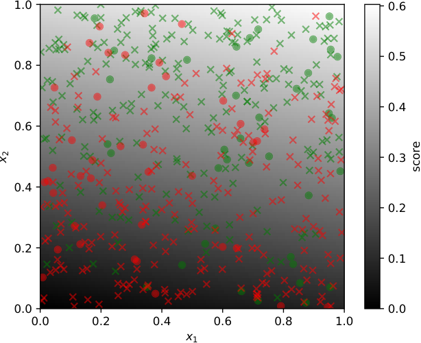
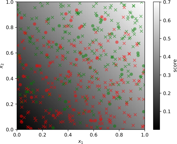
Solving Example 3. Example 3 allows to compare AUC-based and ROC-based approaches. The former uses Eq. 3 as constraint and the latter penalizes $\Delta_{H,3/4}(s)\neq 0$. The goal of our experiment with Example 3 is to show that Algorithm 2 can effectively learn a scoring function $s$ for which the $\alpha$ corresponding to a classifier $g_{s,t_{\alpha}}$ that is fair in FPR is specified in advance, and that the solution can be significantly different from those obtained with AUC-based constraints and Algorithm 1.

We compare the solutions of optimizing the ${\rm AUC}$ without constraint, i.e. Algorithm 1 with $\lambda=0$ with those of Algorithm 1 with $\lambda=1$ and Algorithm 2 where we impose $\Delta_{H,3/4}(s)=0$ with strength $\lambda_{H}=1$. To illustrate the results, we introduce the following family of scoring functions $s_{c}(x)=-c\cdot x_{1}+(1-c)\cdot x_{2}$, parameterized by $c\in[0,1]$.

In practice, we observe that the different constraints lead to scoring functions with specific trade-offs between fairness and performance, as summarized in Table 3. Results with ${\rm AUC}$-based fairness are the same for $\lambda=0$ and $\lambda=1$ because the optimal scoring function for ranking satisfies Eq. 3.

Fig. 10 shows that the ${\rm AUC}$-based constraint has no effect on the solution, unlike the ${\rm ROC}$-based constraint which is successfully enforced by Algorithm 2. Fig. 10 gives two possible scoring functions with Algorithm 2. The median ${\rm ROC}$ curves for two values of $\lambda_{H}$ over 100 independent runs are shown in Fig. 7, with pointwise 95% confidence intervals.

Figure 8: On the left (resp. right), for Example 3, $L_{\lambda}(s_{c})$ (resp. $L_{\Lambda}(s_{c})$) as a function of $c\in[0,1]$ for $\lambda\in\{0,1\}$ (resp. $\lambda_{H}\in\{0,1\}$), with the parametrization $s_{c}(x)=-cx_{1}+(1-c)x_{2}$, and the values $c$ for the scores obtained by gradient descent with Algorithm 1 (resp. Algorithm 2).

(a) $\lambda_{H}=0$

(b) $\lambda_{H}=1$

Figure 9: Values of the output scoring functions on $[0,1]^{2}$ for Algorithm 2 ran on Example 3.

(a) $\lambda_{H}=0$

(b) $\lambda_{H}=1$

Figure 10: Result of Example 3 with Algorithm 2.

Table 3: Results on the test set, averaged over 100 runs (std. dev. are all smaller than $0.02$).

Method	${\rm AUC}$-based fairness					${\rm ROC}$-based fairness
Value of $\lambda$	$\lambda=0$		$\lambda>0$			$\lambda_{H}^{(k)}=\lambda_{H}>0$
	${\rm AUC}$	$\Delta{\rm AUC}$	${\rm AUC}$	$\Delta{\rm AUC}$	$|\Delta_{H,3/4}|$	${\rm AUC}$	$\Delta{\rm AUC}$	$|\Delta_{H,3/4}|$
Example 2	0.79	0.28	0.73	0.00	–	–	–	–
Example 3	0.80	0.02	0.80	0.02	0.38	0.75	0.06	0.00

E.3 Real Data Experiments

Datasets. We evaluate our algorithms on four datasets that have been commonly used in the fair machine learning literature. Those are the following:

• The Compas Dataset (Compas), featured in (Zehlike et al., 2017; Donini et al., 2018), consists in predicting recidivism of convicts in the US. The sensitive variable is the race of the individual, precisely $Z=1$ if the individual is categorized as African-American and $Z=0$ otherwise. It contains 9.4K observations, and we retain 20% of those for testing, and the rest for training/validation. We note that our preprocessing differs from the one used by Donini et al. (2018): in particular, allowing us to retain more data. For completeness, we present in Appendix E.4 the results obtained with the same preprocessing as Donini et al. (2018).

• The Adult Income Dataset (Adult), featured in (Zafar et al., 2019; Donini et al., 2018), is based on US census data and consists in predicting whether income exceeds $50K a year. The sensitive variable is the gender of the individual, i.e. male ($Z=1$) or female ($Z=0$). It contains 32.5K observations for training and validation, as well as 16.3K observations for testing. For simplicity, we removed the weights associated to each instance of the dataset.

• The German Credit Dataset (German), featured in (Zafar et al., 2019; Zehlike et al., 2017; Singh and Joachims, 2019; Donini et al., 2018), consists in classifying people described by a set of attributes as good or bad credit risks. The sensitive variable is the gender of the individual, i.e. male ($Z=1$) or female ($Z=0$). It contains 1,000 instances and we retain 30% of those for testing, and the rest for training/validation.

• The Bank Marketing Dataset (Bank), featured in (Zafar et al., 2019), consists in predicting whether a client will subscribe to a term deposit. The sensitive variable is the age of the individual: $Z=1$ when the age is between 25 and 60 (which we refer to as “working age population”) and $Z=0$ otherwise. It contains 45K observations, of which we retain 20% for testing, and the rest for training/validation.

For all of the datasets, we used one-hot encoding for any categorical variables. The number of training instances $n+m$, test instances $n_{\text{test}}$ and features $d$ for each dataset is summarized in Table 4.

Table 4: Number of observations and feat $d$ per dataset.

Dataset	German	Adult	Compas	Bank
$n+m$	700	32.5K	7.5K	36K
$n_{\text{test}}$	300	16.3K	1.9K	9K
$d$	61	107	16	59

Parameters. For Algorithm 1, we select different ${\rm AUC}$-based fairness constraints for each dataset depending on the semantic of the task. In the case of Compas (recidivism prediction), being labeled positive is a disadvantage so the approach with AUC-based fairness uses the constraint in Eq. 9 to balance FPRs (by forcing the probabilities that a negative from a given group is mistakenly ranked higher than a positive to be the same across groups). Conversely for German (credit scoring), a positive label is an advantage, so we choose Eq. 4 to balance FNRs. For Bank and Adult, the problem has no clear connotation so we select Eq. 5 to force the same ranking accuracy when comparing the positives of a group with the negatives of another.

Inspired by the consideration that many operational settings focus on learning a good score for small FPR rates, the ROC-based approach is configured to simultaneously align the distribution of FPR and TPR for low FPRs between both groups by penalizing solutions with high $|\Delta_{H,1/8}(s)|$, $|\Delta_{H,1/4}(s)|$, $|\Delta_{G,1/8}(s)|$ and $|\Delta_{G,1/4}(s)|$.

Precisely, for every run of Algorithm 2, we set:

$$m_{G}=m_{H}=2,\quad\alpha_{G}^{(1)}=\alpha_{H}^{(1)}=\frac{1}{8},\quad\alpha_{G}^{(1)}=\alpha_{H}^{(2)}=\frac{1}{4},$$

$$\lambda_{G}^{(1)}=\lambda_{G}^{(2)}=\lambda\quad\text{and}\quad\lambda_{H}^{(1)}=\lambda_{H}^{(2)}=\lambda.$$

For all algorithms, we chose the parameter $\lambda$ from the candidate set $\in\{0,0.25,0.5,1,5,10\}$, where $\lambda=0$ corresponds to the case without constraint. Denoting by $\widetilde{s}$ the output of Algorithm 1 or Algorithm 2, we selected the parameter $\lambda_{\text{reg}}$ of the L2 regularization that maximizes the criterion $L_{\lambda}(\widetilde{s})$ (resp. $L_{\Lambda}(\widetilde{s})$) on the validation dataset over the following candidate regularization strength set:

$$\lambda_{\text{reg}}\in\{1\times 10^{-3},5\times 10^{-3},1\times 10^{-2},5\times 10^{-2},1\times 10^{-1},5\times 10^{-1},1\}.$$

The selected parameters are summarized in Table 5. Results are summarized in Table 6, where ${\rm AUC}$ denotes the ranking accuracy ${\rm AUC}_{H_{s},G_{s}}$, and $\Delta{\rm AUC}$ denotes the absolute difference of the terms in the ${\rm AUC}$-based fairness constraint of interest. We also report on the values of $\left\lvert\Delta_{F,1/8}\right\rvert$ and $\left\lvert\Delta_{F,1/4}\right\rvert$ for $F\in\{H,G\}$ and refer the reader to the ${\rm ROC}$ curves in Fig. 11 and Fig. 12 for a visual summary of the other values of $\Delta_{F,\alpha}$ with $F\in\{H,G\}$ and $\alpha\in[0,1]$. We highlight in bold the best ranking accuracy, and the fairest algorithm for the relevant constraint. All of the numerical evaluations reported below are evaluations on the held-out test set.

Table 5: Parameters selected using the validation set for the runs on real data.

Parameters		Constraint
Dataset	Variable	None	${\rm AUC}$	${\rm ROC}$
German	$\lambda$	0	0.25	0.25
	$\lambda_{\text{reg}}$	0.5	0.5	0.5
Adult	$\lambda$	0	0.25	0.25
	$\lambda_{\text{reg}}$	0.05	0.05	0.05
Compas	$\lambda$	0	0.5	0.25
	$\lambda_{\text{reg}}$	0.05	0.05	0.05
Bank	$\lambda$	0	0.25	0.25
	$\lambda_{\text{reg}}$	0.05	0.05	0.05

Table 6: Results on test set. The strength of fairness constraints and regularization is chosen based on a validation set to obtain interesting trade-offs, as detailed in Section E.3.

Measure		Dataset
Constraint	Value	German	Adult	Compas	Bank
None	${\rm AUC}$	0.76	0.91	0.72	0.94
	$\Delta{\rm AUC}$	0.07	0.16	0.20	0.13
	$|\Delta_{H,1/8}|$	0.01	0.31	0.26	0.09
	$|\Delta_{H,1/4}|$	0.20	0.36	0.32	0.18
	$|\Delta_{G,1/8}|$	0.13	0.02	0.29	0.00
	$|\Delta_{G,1/4}|$	0.20	0.06	0.29	0.04
${\rm AUC}$-based	${\rm AUC}$	0.75	0.89	0.71	0.93
	$\Delta{\rm AUC}$	0.05	0.02	0.00	0.05
	$|\Delta_{H,1/8}|$	0.05	0.09	0.06	0.03
	$|\Delta_{H,1/4}|$	0.08	0.17	0.03	0.11
	$|\Delta_{G,1/8}|$	0.01	0.06	0.02	0.27
	$|\Delta_{G,1/4}|$	0.02	0.14	0.06	0.37
${\rm ROC}$-based	${\rm AUC}$	0.75	0.87	0.70	0.91
	$\Delta{\rm AUC}$	0.07	0.07	0.05	0.14
	$|\Delta_{H,1/8}|$	0.03	0.06	0.01	0.03
	$|\Delta_{H,1/4}|$	0.07	0.01	0.02	0.05
	$|\Delta_{G,1/8}|$	0.04	0.00	0.00	0.06
	$|\Delta_{G,1/4}|$	0.01	0.02	0.00	0.21

Figure 11: ${\rm ROC}$ curves for Bank and German for a score learned without and with fairness constraints. On all plots, dashed and solid lines represent respectively training and test sets. Black curves represent ${\rm ROC}_{H_{s},G_{s}}$, and above the curves we report the corresponding ranking performance ${\rm AUC}_{H_{s},G_{s}}$.

Results for the datasets Compas and Adult. These results are presented in Section 5 of the main text. For completeness, Fig. 12 represents ${\rm ROC}$ curves on the training set of Compas and Adult, on top of the test set ${\rm ROC}$ curves already displayed in Fig. 3 of the main text.

Results for the dataset Bank. Recall that for this dataset we consider the ${\rm AUC}$ constraint Eq. 5 to force the same ranking accuracy when comparing the positives of a group with the negatives of another. Fig. 11 shows that the score learned without constraint implies a stochastic order between the distributions of the problem that writes $H_{s}^{(1)}\preceq H_{s}^{(0)}\preceq G_{s}^{(0)}\preceq G_{s}^{(1)}$, where $h\preceq g$ means that $g$ is stochastically larger than $h$ (Fig. 11-b). This suggests that the task of distinguishing positives from negatives is much harder for observations of the group $Z=0$ than for those of the working age population ($Z=1$), which could be a consequence of the heterogeneity of the group $Z=0$. On the other hand, the left plot representing ${\rm ROC}_{H_{s}^{(1)},G_{s}^{(0)}}$ and ${\rm ROC}_{H_{s}^{(0)},G_{s}^{(1)}}$ (Fig. 11-a) for the setting without constraint gives an appreciation of the magnitude of those differences. Precisely, it implies that it is much harder to distinguish working age positives ($Y=+1,Z=1$) from negatives of group $Z=0$ than working age negatives from positives of group $Z=0$ (Fig. 11-a). The correction induced by the ${\rm AUC}$ constraint suggests that it was due to the fact that scores for positives of the group ($Y=+1,Z=0$) were too small compared to the positives of the working age population ($Y=+1,Z=1$). Indeed, learning with the ${\rm AUC}$ constraint roughly equalizes the scores of the positives across both groups $Z=0$ and $Z=1$ (Fig. 11-d). Additionally, in the left plot for learning with ${\rm AUC}$ constraints, we can see that ${\rm ROC}_{H_{s}^{(1)},G_{s}^{(0)}}$ and ${\rm ROC}_{H_{s}^{(0)},G_{s}^{(1)}}$ intersect and have similar ${\rm AUC}$’s as expected (Fig. 11-c), which is more visible for the dashed lines (i.e. on training data). Finally, the ${\rm ROC}$-based constraint induces as expected the equality of $G_{s}^{(0)}$ and $G_{s}^{(1)}$ as well as that of $H_{s}^{(0)}$ and $H_{s}^{(1)}$ in the high score regime, as seen on the right plot (Fig. 11-f). It implies that ${\rm ROC}_{H_{s}^{(1)},G_{s}^{(0)}}$ and ${\rm ROC}_{H_{s}^{(0)},G_{s}^{(1)}}$ are much closer for simultaneously small TPR’s and FPR’s (Fig. 11-e), which entails that thresholding top scores will yield fair classifiers in FPR and TPR again for a whole range of high thresholds.

Results for the dataset German. Recall that for this credit scoring dataset we consider the ${\rm AUC}$-based constraint in Eq. 4 to force the probabilities that a positive from a given group is mistakenly ranked higher than a negative to be the same across groups. Despite the blatant issues of generalization due to the very small size of the dataset (see Table 4), we see in Fig. 11 that the learned score without fairness constraints systematically makes more errors for women with good ground truth credit risk, as can be seen from comparing ${\rm ROC}_{H_{s},G_{s}^{(0)}}$ and ${\rm ROC}_{H_{s},G_{s}^{(1)}}$ (Fig. 11-g) Additionally, the credit score of men with good or bad credit risk is in both cases stochastically larger than that of women of the same credit risk assessment (see ${\rm ROC}_{G_{s}^{(0)},G_{s}^{(1)}}$ and ${\rm ROC}_{H_{s}^{(0)},H_{s}^{(1)}}$ in Fig. 11-h). On the other hand, the score learned with an ${\rm AUC}$ constraint makes a similar amount of mistakes for both genders, with only slightly more mistakes made on men than women (Fig. 11-i), and the scores $s(X)$ conditioned on the events $(Y=y,Z=z)$ with $z=0$ and $z=1$ are more aligned when considering both $y=-1$ and $y=+1$ (Fig. 11-j). Finally, while the score learned with a ${\rm ROC}$ constraint has a slightly higher discrepancy between the ${\rm AUC}$’s involved in Eq. 4 than the one learned with an ${\rm AUC}$ constraint (Fig. 11-k), one observes that both pairs of distributions $(G_{s}^{(0)},G_{s}^{(1)})$ and $(H_{s}^{(0)},H_{s}^{(1)})$ are equal for high thresholds (Fig. 11-l). Consistently with the results on other datasets, this suggests that our score leads to classifiers that are fair in FPR and TPR for a whole range of problems where one selects individuals with very good credit risks by thresholding top scores.

Figure 12: ${\rm ROC}$ curves for Adult and Compas for a score learned without and with fairness constraints. On all plots, dashed and solid lines represent respectively training and test sets. Black curves represent ${\rm ROC}_{H_{s},G_{s}}$, and above the curves we report the corresponding ranking performance ${\rm AUC}_{H_{s},G_{s}}$.

E.4 Results on Compas with a Different Preprocessing

For the dataset Compas, the results in Section 5 use a different preprocessing from Donini et al. (2018) which allows us to retain more data. For completeness, we perform additional experiments using the same data and preprocessing as Donini et al. (2018). The main difference is that the sensitive variable to be $Z=1$ if an individual is categorized as African-American and $Z=0$ if it is categorized as Caucasian (observations associated with other ethnicities are discarded). The dataset then contains 5.3K observations ($n+m$), and we retained 20% of those for testing, and the rest for training/validation. Results are reported in Fig. 13.

Figure 13: ${\rm ROC}$ curves for Compas for the preprocessing described in Donini et al. (2018), and a score learned without and with fairness constraints. On all plots, dashed and solid lines represent respectively training and test sets. Black curves represent ${\rm ROC}_{H_{s},G_{s}}$, and above the curves we report the corresponding ranking performance ${\rm AUC}_{H_{s},G_{s}}$.

References

- Abadi et al. (2016) M. Abadi, A. Agarwal, P. Barham, E. Brevdo, Z. Chen, C. Citro, G. S. Corrado, A. Davis, J. Dean, M. Devin, S. Ghemawat, I. J. Goodfellow, A. Harp, G. Irving, M. Isard, Y. Jia, R. Józefowicz, L. Kaiser, M. Kudlur, J. Levenberg, D. Mané, R. Monga, S. Moore, D. G. Murray, C. Olah, M. Schuster, J. Shlens, B. Steiner, I. Sutskever, K. Talwar, P. A. Tucker, V. Vanhoucke, V. Vasudevan, F. B. Viégas, O. Vinyals, P. Warden, M. Wattenberg, M. Wicke, Y. Yu, and X. Zheng. Tensorflow: Large-scale machine learning on heterogeneous distributed systems, 2016.
- Agarwal et al. (2018) A. Agarwal, A. Beygelzimer, M. Dudík, J. Langford, and H. M. Wallach. A reductions approach to fair classification. In Proceedings of the 35th International Conference on Machine Learning, volume 80 of Proceedings of Machine Learning Research, pages 60–69. PMLR, 2018.
- Agarwal et al. (2005) S. Agarwal, T. Graepel, R. Herbrich, S. Har-Peled, and D. Roth. Generalization bounds for the area under the ROC curve. Journal of Machine Learning Research, 6:393–425, 2005.
- Bechavod and Ligett (2017) Y. Bechavod and K. Ligett. Learning fair classifiers: A regularization-inspired approach. CoRR, abs/1707.00044, 2017.
- Beutel et al. (2019) A. Beutel, J. Chen, T. Doshi, H. Qian, L. Wei, Y. Wu, L. Heldt, Z. Zhao, L. Hong, E. H. Chi, and C. Goodrow. Fairness in recommendation ranking through pairwise comparisons. In Proceedings of the 25th ACM SIGKDD International Conference on Knowledge Discovery & Data Mining, KDD 2019, pages 2212–2220. ACM, 2019.
- Biega et al. (2018) A. J. Biega, K. P. Gummadi, and G. Weikum. Equity of attention: Amortizing individual fairness in rankings. In The 41st International ACM SIGIR Conference on Research & Development in Information Retrieval, SIGIR 2018, pages 405–414. ACM, 2018.
- Borkan et al. (2019) D. Borkan, L. Dixon, J. Sorensen, N. Thain, and L. Vasserman. Nuanced metrics for measuring unintended bias with real data for text classification. In Companion of The 2019 World Wide Web Conference (WWW), 2019.
- Boucheron et al. (2005) S. Boucheron, O. Bousquet, and G. Lugosi. Theory of classification : a survey of some recent advances. ESAIM: Probability and Statistics, 9:323–375, 2005.
- Bousquet et al. (2003) O. Bousquet, S. Boucheron, and G. Lugosi. Introduction to statistical learning theory. In Advanced Lectures on Machine Learning, ML Summer Schools 2003, volume 3176 of Lecture Notes in Computer Science, pages 169–207. Springer, 2003.
- Celis et al. (2018) L. E. Celis, D. Straszak, and N. K. Vishnoi. Ranking with fairness constraints. In 45th International Colloquium on Automata, Languages, and Programming, ICALP 2018, volume 107 of LIPIcs, pages 28:1–28:15. Schloss Dagstuhl - Leibniz-Zentrum für Informatik, 2018.
- Chen (2018) J. Chen. Fair lending needs explainable models for responsible recommendation. CoRR, abs/1809.04684, 2018.
- Chzhen et al. (2020) E. Chzhen, C. Denis, M. Hebiri, L. Oneto, and M. Pontil. Fair Regression via Plug-in Estimator and Recalibration With Statistical Guarantees. HAL, archives ouvertes, Mar. 2020.
- Clémençon and Vayatis (2007) S. Clémençon and N. Vayatis. Ranking the best instances. Journal of Machine Learning Research, 8:2671–2699, 2007.
- Clémençon and Vayatis (2009) S. Clémençon and N. Vayatis. Tree-based ranking methods. IEEE Transactions on Information Theory, 55(9):4316–4336, 2009.
- Clémençon and Vayatis (2010) S. Clémençon and N. Vayatis. The RankOver algorithm: overlaid classification rules for optimal ranking. Constructive Approximation, 32:619–648, 2010.
- Clémençon et al. (2011) S. Clémençon, M. Depecker, and N. Vayatis. Adaptive partitioning schemes for bipartite ranking. Machine Learning, 83(1):31–69, 2011.
- Clémençon et al. (2016) S. Clémençon, I. Colin, and A. Bellet. Scaling-up Empirical Risk Minimization: Optimization of Incomplete -statistics. Journal of Machine Learning Research, 17(76):1–36, 2016.
- Clémençon and Vayatis (2009) S. Clémençon and N. Vayatis. Nonparametric estimation of the precision-recall curve. In Proceedings of the 26th Annual International Conference on Machine Learning, ICML 2009, volume 382 of ACM International Conference Proceeding Series, pages 185–192. ACM, 2009.
- Clémençon et al. (2008) S. Clémençon, G. Lugosi, and N. Vayatis. Ranking and Empirical Minimization of U-Statistics. The Annals of Statistics, 36(2):844–874, 2008.
- Clémençon et al. (2009) S. Clémençon, M. Depecker, and N. Vayatis. AUC optimization and the two-sample problem. In Advances in Neural Information Processing Systems 22: 23rd Annual Conference on Neural Information Processing Systems 2009, pages 360–368. Curran Associates, Inc., 2009.
- Deo (2015) R. Deo. Machine learning in medicine. Circulation, 132(20):1920–1930, 2015.
- Donini et al. (2018) M. Donini, L. Oneto, S. Ben-David, J. Shawe-Taylor, and M. Pontil. Empirical risk minimization under fairness constraints. In Advances in Neural Information Processing Systems 31: Annual Conference on Neural Information Processing Systems 2018, NeurIPS 2018, pages 2796–2806, 2018.
- Dwork et al. (2012) C. Dwork, M. Hardt, T. Pitassi, O. Reingold, and R. S. Zemel. Fairness through awareness. In Innovations in Theoretical Computer Science 2012, pages 214–226. ACM, 2012.
- Goodfellow et al. (2016) I. Goodfellow, Y. Bengio, and A. Courville. Deep Learning. MIT Press, 2016.
- Grother and Ngan (2019) P. Grother and M. Ngan. Face Recognition Vendor Test (FRVT) — Performance of Automated Gender Classification Algorithms. Technical Report NISTIR 8052, National Institute of Standards and Technology (NIST), 2019.
- Györfi (2002) L. Györfi. Principles of Nonparametric Learning. Springer, 2002.
- Hardt et al. (2016) M. Hardt, E. Price, and N. Srebro. Equality of opportunity in supervised learning. In Advances in Neural Information Processing Systems 29: Annual Conference on Neural Information Processing Systems 2016, pages 3315–3323, 2016.
- Hsieh and Turnbull (1996) F. Hsieh and B. W. Turnbull. Nonparametric and semiparametric estimation of the receiver operating characteristic curve. The Annals of Statistics, 24(1):25–40, 1996.
- Kallus and Zhou (2019) N. Kallus and A. Zhou. The fairness of risk scores beyond classification: Bipartite ranking and the XAUC metric. In Advances in Neural Information Processing Systems 32: Annual Conference on Neural Information Processing Systems 2019, NeurIPS 2019, pages 3433–3443. 2019.
- Kleinberg et al. (2017) J. M. Kleinberg, S. Mullainathan, and M. Raghavan. Inherent trade-offs in the fair determination of risk scores. In 8th Innovations in Theoretical Computer Science Conference, ITCS 2017, volume 67 of LIPIcs, pages 43:1–43:23. Schloss Dagstuhl - Leibniz-Zentrum für Informatik, 2017.
- Lee (1990) A. J. Lee. -statistics: Theory and practice. Marcel Dekker, Inc., New York, 1990.
- Menon and Williamson (2016) A. K. Menon and R. C. Williamson. Bipartite ranking: a risk-theoretic perspective. Journal of Machine Learning Research, 17(195):1–102, 2016.
- Menon and Williamson (2018) A. K. Menon and R. C. Williamson. The cost of fairness in binary classification. In Conference on Fairness, Accountability and Transparency, FAT 2018, volume 81 of Proceedings of Machine Learning Research, pages 107–118. PMLR, 2018.
- Papa et al. (2015) G. Papa, S. Clémençon, and A. Bellet. SGD algorithms based on incomplete u-statistics: Large-scale minimization of empirical risk. In Advances in Neural Information Processing Systems 28: Annual Conference on Neural Information Processing Systems 2015, pages 1027–1035, 2015.
- Pedregosa et al. (2011) F. Pedregosa, G. Varoquaux, A. Gramfort, V. Michel, B. Thirion, O. Grisel, M. Blondel, P. Prettenhofer, R. Weiss, V. Dubourg, J. Vanderplas, A. Passos, D. Cournapeau, M. Brucher, M. Perrot, and E. Duchesnay. Scikit-learn: Machine learning in Python. Journal of Machine Learning Research, 12:2825–2830, 2011.
- Pleiss et al. (2017) G. Pleiss, M. Raghavan, F. Wu, J. M. Kleinberg, and K. Q. Weinberger. On fairness and calibration. In Advances in Neural Information Processing Systems 30: Annual Conference on Neural Information Processing Systems 2017, pages 5680–5689, 2017.
- Ruder (2016) S. Ruder. An overview of gradient descent optimization algorithms. CoRR, abs/1609.04747, 2016.
- Rudin (2006) C. Rudin. Ranking with a p-norm push. In Learning Theory, 19th Annual Conference on Learning Theory, COLT 2006, volume 4005 of Lecture Notes in Computer Science, pages 589–604. Springer, 2006.
- Rudin et al. (2018) C. Rudin, C. Wang, and B. Coker. The age of secrecy and unfairness in recidivism prediction. CoRR, abs/1811.00731, 2018.
- Shorack and Wellner (1989) G. Shorack and J. A. Wellner. Empirical Processes with applications to Statistics. Classics in Applied Mathematics. SIAM, 1989.
- Singh and Joachims (2018) A. Singh and T. Joachims. Fairness of exposure in rankings. In Proceedings of the 24th ACM SIGKDD International Conference on Knowledge Discovery & Data Mining, KDD 2018, pages 2219–2228. ACM, 2018.
- Singh and Joachims (2019) A. Singh and T. Joachims. Policy learning for fairness in ranking. In Advances in Neural Information Processing Systems 32: Annual Conference on Neural Information Processing Systems 2019, NeurIPS 2019, pages 5427–5437, 2019.
- van der Vaart (2000) A. W. van der Vaart. Asymptotic Statistics. Cambridge Series in Statistical and Probabilistic Mathematics, 2000.
- van der Vaart and Wellner (1996) A. W. van der Vaart and J. a. Wellner. Weak convergence and empirical processes. 1996.
- Vogel et al. (2018) R. Vogel, A. Bellet, and S. Clémençon. A probabilistic theory of supervised similarity learning for pointwise ROC curve optimization. In Proceedings of the 35th International Conference on Machine Learning, ICML 2018, volume 80 of Proceedings of Machine Learning Research, pages 5062–5071. PMLR, 2018.
- Woodworth et al. (2017) B. E. Woodworth, S. Gunasekar, M. I. Ohannessian, and N. Srebro. Learning non-discriminatory predictors. In Proceedings of the 30th Conference on Learning Theory, COLT 2017, volume 65 of Proceedings of Machine Learning Research, pages 1920–1953. PMLR, 2017.
- Zafar et al. (2017a) M. B. Zafar, I. Valera, M. Gomez-Rodriguez, and K. P. Gummadi. Fairness beyond disparate treatment & disparate impact: Learning classification without disparate mistreatment. In Proceedings of the 26th International Conference on World Wide Web, WWW 2017, pages 1171–1180. ACM, 2017a.
- Zafar et al. (2017b) M. B. Zafar, I. Valera, M. Gomez-Rodriguez, and K. P. Gummadi. Fairness constraints: Mechanisms for fair classification. In Proceedings of the 20th International Conference on Artificial Intelligence and Statistics, AISTATS 2017, volume 54 of Proceedings of Machine Learning Research, pages 962–970. PMLR, 2017b.
- Zafar et al. (2019) M. B. Zafar, I. Valera, M. Gomez-Rodriguez, and K. P. Gummadi. Fairness constraints: A flexible approach for fair classification. Journal of Machine Learning Research, 20(75):1–42, 2019.
- Zehlike et al. (2017) M. Zehlike, F. Bonchi, C. Castillo, S. Hajian, M. Megahed, and R. Baeza-Yates. Fa*ir: A fair top-k ranking algorithm. In Proceedings of the 2017 ACM on Conference on Information and Knowledge Management, CIKM 2017, pages 1569–1578. ACM, 2017.
- Zhao et al. (2011) P. Zhao, S. C. H. Hoi, R. Jin, and T. Yang. Online AUC maximization. In Proceedings of the 28th International Conference on Machine Learning, ICML 2011, pages 233–240. Omnipress, 2011.