Probing Dark Matter with Future CMB Measurements

Abstract

The annihilation and decay of dark matter (DM) during the dark ages can leave imprints in the Cosmic Microwave Background Radiation (CMB) by altering the cosmic reionization process. CMB polarization anisotropy can be sensitive to such energy injection at higher redshift and therefore helps reducing degeneracy between spectral parameters in $\Lambda$CDM and other astrophysical parameters. In light of several upcoming CMB polarization experiments, such as AdvACTPol, AliCPT, CLASS, Simons Observatory, Simons Array, SPT-3G, we forecast their prospective sensitivity in probing dark matter annihilation and decay signals. We find that future missions have 95% C.L. projected limits on DM decay and annihilation rates to orders of $\Gamma_{\chi}(\tau_{\chi}^{-1})\sim 10^{-27}{~\rm{s}}^{-1}$ and $\left<\sigma v\right>/m_{\chi}\sim 10^{-29}{~\rm{cm^{3}s^{-1}GeV^{-1}}}$ respectively, significantly improving the sensitivity to DM from current experimental bounds.

I Introduction

The majority of matter in the Universe exists in the form of non-luminous, non-baryonic Cold Dark Matter (CDM). A Weakly Interacting Massive Particle (WIMP) is a well-motivated particle physics candidate that explains the relic abundance of the Universe. Tremendous efforts have been invested for WIMP dark matter searches using terrestrial or space-borne experiments, see Refs. Cushman et al. 2013; Profumo 2013; Boveia and Doglioni 2018; Schumann 2019 for recent reviews. In addition to dedicated direct and indirect searches, the Cosmic Microwave Background (CMB) also provides an avenue for WIMP detection Chen and Kamionkowski 2004; Adams et al. 1998; Padmanabhan and Finkbeiner 2005; Pierpaoli 2004, which has gained increasing interest Acharya and Khatri 2019; Aghanim et al. 2018; Slatyer and Wu 2017; Slatyer 2016a; Liu et al. 2016; Kawasaki et al. 2016, especially with the availability of precision data from Planck Aghanim et al. 2019; Aghanim et al. 2016 experiment.

Thermally produced WIMP dark matter generally may annihilate or decay into the SM particles that subsequently become electromagnetically interacting electrons and photons. During the cosmic dark ages, this extra budget of energetic particle injection can heat up and ionize an amount of the neutral baryonic gas. Increased fraction of free electrons enhances the scattering of CMB photons during its propagation that leaves measurable imprints on the temperature and polarization anisotropy spectra of CMB. High-precision CMB measurement can place stringent limits on post-recombination annihilation and decay for dark matter over a wide mass range. The latest Planck 2018 results Aghanim et al. 2018 report constraints on weak-scale DM annihilation cross-section that is comparable to the diffuse gamma-ray bound given by the combined analysis of Fermi-LAT and MAGIC data Ahnen et al. 2016. Besides, the relatively lower energy requirement for hydrogen ionization allows such limits to extend into much smaller mass ranges, effectively filling the gap between X-ray and gamma-ray indirect searches.

Energy injection from dark matter modifies CMB anisotropy mostly via the ionization of intergalactic medium (IGM). In the temperature anisotropy spectrum, such injection is known to degenerate with several cosmological parameters Padmanabhan and Finkbeiner 2005 , such as the amplitude and tilt of primordial scalar perturbation ($A_{\rm{s}}$, $n_{\rm{s}}$), and the optical depth ($\tau$). Polarization anisotropy spectra help to break these degeneracies and gives tighter DM constraints. The Planck 2018 data Aghanim et al. 2019 provided the most stringent bounds on the cosmological parameters by far. Its constraints on DM annihilation cross-section by temperature anisotropy is tightened by about one order of magnitude with its polarization (EE) and cross-correlation (TE) spectra.

A number of operating or planned CMB experiments are expected to offer higher precision polarization data that may further enhance the sensitivity to dark matter annihilation and decay. These experiments include BICEP3/KECK Array Grayson et al. 2016 and South Pole Telescope-3G Anderson et al. 2018 in Antarctica, Advanced Atacama Cosmology Telescope Polarimeter (AdvACTPol) Calabrese et al. 2014; Li et al. 2018a, Cosmology Large Angular Scale Surveyor(CLASS) Essinger-Hileman et al. 2014, Simons Array Suzuki et al. 2016; Arnold et al. 2014 and Simons Observatory Ade et al. 2019 in Chile, and Ali CMB Polarization Telescope (AliCPT) Li et al. 2017 in China that aims at the northern hemisphere.

In this paper, we investigate the WIMP detection prospects of the upcoming CMB polarization experiments in a mass range of 10 KeV - 10 TeV, where the WIMPs are heavy enough so that their annihilation and decay products can efficiently ionize the neutral gas of the Universe. In the following Section II we briefly discuss the energy injection and deposition as well as the late-time clustering enhancement in annihilation rate. Section III discusses the impact of energy injection on the recombination history and CMB anisotropy and the breaking parameter degeneracies by polarization spectra. Section  IV presents our forecasting method and analysis results, then we conclude in Section V.

II Energy injection and deposition

Assuming dark matter $\chi$ converts all its mass into the energy of annihilation and decay products, the energy injection rate per unit volume is

$$\left(\frac{{\rm{d}}E}{{\rm{d}}V{\rm{d}}t}\right)_{\rm{INJ}}\ =\left\{\begin{array}[]{l}m_{\chi}\Gamma_{\chi}n_{\chi}e^{-\Gamma_{\chi}t}\ \ \ \ \ \ \ \ {\rm{decay}}\\ {g}\cdot 2m_{\chi}n_{\chi}^{2}\left<\sigma v\right>\ \ \ {\rm{annihilation}}\end{array}\right.$$ (1)

where $\Gamma_{\chi}$ is the DM decay width, defined as the inverse of decay lifetime ( $\Gamma_{\chi}=\tau_{\chi}^{-1}$). $g$ is a symmetry factor that equals 1/2 for self-conjugate dark matter, and 1/4 otherwise due to halving the number density between $\chi$ and $\bar{\chi}$. We will take $g=1/2$ throughout this paper. $\left<\sigma v\right>$ is the thermally averaged annihilation cross section, here we only consider $s$-wave annihilation for which $\left\langle\sigma v\right\rangle$ is invariant. The average DM number density $n_{\chi}=\rho_{\rm{c}}\Omega_{\chi}(1+z)^{3}/m_{\chi}$, where $\Omega_{\chi},\rho_{\rm c}$ are the cold dark matter fraction and the critical density of the Universe today. As the relevant decay lifetime are much longer than the age of Universe, hereafter we will ignore the factor $e^{-\Gamma_{\chi}t}$ in Eq.(1). The redshift dependent injection rates can be written as

$$\left(\frac{{\rm{d}}E}{{\rm{d}}V{\rm{d}}t}\right)_{\rm{INJ}}^{\rm{dec}}\ = \ \Gamma_{\chi}\Omega_{\chi}(1+z)^{3}\rho_{\rm{c}}$$ (2)

$$\left(\frac{{\rm{d}}E}{{\rm{d}}V{\rm{d}}t}\right)_{\rm{INJ}}^{\rm{ann}}\ = \ \frac{\left<\sigma v\right>}{m_{\chi}}\Omega_{\chi}^{2}(1+z)^{6}\rho_{\rm{c}}^{2}$$ (3)

note that homogeneous DM distribution is assumed in Eq.(3). The DM annihilation injection rate decreases faster as the Universe expands due to its dependence on higher power of $z$ . As will be discussed later, the annihilation rate will be boosted at late time by the DM clustering after the formation of halos. In comparison, DM decay yields a more steady rate of energy injection.

The final cascaded state of the annihilation and decay produces a variety of standard -model particles. Over the Hubble time-scale, these metastable products eventually decay into stable particles such as photons, electrons, protons and neutrinos. The injection of energy into the intergalactic medium is dominated by electrons and photons. Neutrinos do not interact efficiently with baryonic matter and decouple from the picture, protons are subdominant in abundance and can be ignored Weniger et al. 2013.

The energetic photon and electrons lose their energy due to cosmic expansion, and also in a series of absorption and scattering processes with the CMB photons and the baryonic matter (mostly neutral gas). Interested readers can refer to Kawasaki et al. 2016; Slatyer et al. 2009; Slatyer 2013; Belotsky and Kirillov 2015; Liu et al. 2019 for recent studies on the propagation and energy deposit of injected particles. Distortion in the CMB anisotropy is mostly due to increased ionization, and the most relevant energy deposit channels are

• Direct ionization of ground-state neutral hydrogen;

• Excitation of the neutral hydrogen atom from $1s$ to $2p$ state, contributing to indirect ionization.

A handful of other energy loss channels are less effective in altering the anisotropy spectra. For example, energy deposit into heating the IGM can cause a dramatic rise in the gas temperature at low redshift, yet the impact on anisotropy spectra is insignificant compared to ionization channels. Contribution from helium ionization is found to be subdominant compared to hydrogen Liu et al. 2016 and will not be included in our calculation. A fraction of injected energy can also be deposited into changing the energy spectrum of CMB.

For highly relativistic injected particles, their energy deposition is a gradual process that continues to later times. For a given redshift, an effective efficiency $f_{\rm{c}}$ represents the ratio between the rate of energy deposition to that of DM injection at the same redshift,

$$\left(\frac{{\rm{d}}E}{{\rm{d}}V{\rm{d}}t}\right)_{\rm{DEP,c}}\ =\ f_{\rm{c}}\left(\frac{{\rm{d}}E}{{\rm{d}}V{\rm{d}}t}\right)_{\rm{INJ}}$$ (4)

here the subscript c labels the deposition channel, DEP and INJ refer to deposition and injection rates respectively. The deposition efficiency $f_{\rm{c}}$ depends on the particle species, its energy upon injection, the redshift, and accumulates over particles injected at earlier times. A previously popular scheme uses an “SSCK” prescription Shull and van Steenberg 1985; Chen and Kamionkowski 2004; Slatyer 2016a that assumes a fraction $(1-x_{\rm{e}})/3$ of the energy deposit goes into ionization. Here, we will adopt $f_{\rm{c}}$ from recent numerical analyses.

II.1 Deposition efficiency

The effective energy deposition efficiency $f_{\rm{c}}$ can be constructed from a discretized deposit fraction coefficient $T_{{\rm{c}},ijk}(z_{i},E_{j},z_{k})$ over redshift and energy bins, as given in Ref. Slatyer 2016b, which describes the fraction of $E_{j}$ deposited into channel $\rm{c}$ at redshift $z_{i}$, where $E_{j}$ is the particle’s initial kinetic energy at its injection redshift $z_{k}$. $f_{\rm{c}}(z_{i})$ is obtained by summing $T$ over all injection redshift bins prior to $z_{i}$,

$$f_{\rm{c}}(z_{i})\approx\frac{\sum_{j}\sum_{k}A_{jk}{\rm d}V(z_{k}){\rm d}t(z_{k})T_{{\rm c},ijk}}{\sum_{j}A_{ji}{\rm d}V(z_{i}){\rm d}t(z_{i})}$$ (5)

where

$$A_{jk}=E_{j}\left(\frac{{\rm d}N}{{\rm d}E_{j}{\rm d}V(z_{k}){\rm d}t(z_{k})}\right){\rm d}E_{j}$$ (6)

In Eq. (5), ${\rm{d}}t(z)$ is the time interval corresponding to ${\rm{d}}\ln(1+z)=10^{-3}$. The numerator sums over the contribution from the earlier injection, and the denominator gives the total energy injection at $z_{i}$. From Eq.(5) it is clear that $f_{\rm{c}}$ for annihilation and decay scenarios are differently weighted over historical deposits. Also, $f_{\rm{c}}$ may exceed unity at the late time due to accumulated injection.

We will consider direct production of $e^{\pm}$ and $\gamma\gamma$, for which the injection spectrum is monochromatic (at $E_{j}$),

$$\frac{{\rm{d}}N}{{\rm{d}}E{\rm{d}}V{\rm{d}}t}=\frac{1}{E_{j}}\left(\frac{{\rm{d}}E}{{\rm{d}}V{\rm{d}}t}\right)_{\rm{INJ}}\delta_{\rm{D}}(E-E_{j})$$ (7)

where $\delta_{\rm{D}}$ refers to Dirac delta function. Eq.(5) can then be simplified as

$$f_{\rm{c}}(z_{i},E_{j})=\frac{H(z_{i})}{(1+z_{i})^{\beta}}\sum_{k}\frac{T_{{\rm c},ijk}{(1+z_{k})^{\beta}}}{H(z_{k})}$$ (8)

where $\beta=0$ for DM decay and $\beta=3$ for DM annihilation, note that we used $H(z)=-{\rm{d}}\ln(1+z)/{\rm{d}}t$.

II.2 Clustering enhancement

Structure formation at low $z$ let DM cluster into halos, and the DM density condensation enhances DM annihilation due to $\rho^{2}$ dependence. This enhancement over unclustered average-density annihilation is formulated as a ‘boost factor’ $B(z)$ Liu et al. 2016,

$$\left(\frac{{\rm{d}}E}{{\rm{d}}V{\rm{d}}t}\right)^{\rm{ann,boosted}}_{\rm{INJ}}\ =\ \left[1+B(z)\right]\ \left(\frac{{\rm{d}}E}{{\rm{d}}V{\rm{d}}t}\right)^{\rm{ann}}_{\rm{INJ}}$$ (9)

The overall boost is obtained by integrating over the contribution from halos Taylor and Silk 2003,

$$B(z)=\frac{\Delta_{\rm c}\rho_{\rm c}}{\rho^{2}_{\rm{DM}}}\int^{\infty}_{M_{\rm min}}MB_{\rm h}(M)\frac{{\rm{d}}n}{{\rm{d}}M}{\rm{d}}M$$ (10)

where $\Delta_{\rm c}\rho_{\rm c}$ is the average density of bound halos, in subsequent analysis we will assume $\Delta_{\rm c}=200$ and use a cut-off of $M_{\rm{min}}=10^{-6}\rm{M}_{\odot}$ as a reasonable estimate for the minimum halo mass. $B_{\rm{h}}(M)$ is the enhancement from an individual halo of mass $M$,

$$B_{\rm h}(M)=\frac{4\pi}{\bar{\rho}_{\rm h}^{2}V_{\rm h}(M)}\int^{r_{200}}_{0}{\rm{d}}r\rho^{2}(r)r^{2}$$ (11)

here $\bar{\rho}_{\rm h}$ gives the average density of the halo distributed within volume $V_{\rm h}(M)$. $\rho(r)$ describes the radial density profile, truncated at a virial radius $r_{200}$. We consider spherical collapse model of halo formation, for which the mass function is given by Ref. Schneider et al. 2013; Sheth and Tormen 1999,

$$\frac{{\rm{d}}n}{{\rm{d}}\ln M} = \frac{1}{2}f({\rm{\nu}})\frac{\rho_{\rm{DM}}}{M}\frac{{\rm{d}}\ln({\rm{\nu}})}{{\rm{d}}\ln M}$$ (12)

$$f({\rm{\nu}}) = A\sqrt{\frac{2q{\rm{\nu}}}{\pi}}[1+(q{\rm{\nu}})^{-p}]\ {\rm{e}}^{-q{\rm{\nu}}/2}$$ (13)

with $A=0.3222$, $p=0.3$, $q=0.707$ and the scaled variable $\nu\equiv[\delta_{\rm{cr}}/(\sigma(M)D(z))]^{2}$, where $\delta_{\rm{cr}}\approx 1.686$, $\sigma(M)$ is the rms linear over-density and $D(z)$ is the growth factor normalized to unity today.

We ignored further boost from halo substructures and used a typical cuspy Einasto profile Einasto 1965 for the main halo,

$$\rho(r)=\rho_{-2}\ {\rm exp}\left({-\frac{2}{\alpha_{\rm{e}}}\left[\left(\frac{r}{r_{-2}}\right)^{\alpha_{\rm{e}}}-1\right]}\right)$$ (14)

where $\rho_{-2}$, $r_{-2}$, $\alpha_{\rm{e}}$ are halo profile parameters, assumed to follow the empirical relations given in Ref. Klypin et al. 2016, $\alpha_{\rm e}=0.115+0.0165\mu^{2}$, and $r_{200}/r_{-2}=6.5\mu^{-1.6}(1+0.21\mu^{2})$, where $\mu\equiv\delta_{\rm{cr}}/\sigma(M)$. $B(z)$ reaches unity around $z=45$ and increases dramatically afterwards, giving $B=783$ at $z=20$. Having acquired the boost factor, we can account for the clustering enhancement by using a ‘boosted’ version of the deposition efficiency for annihilation,

$$f_{\rm{c}}^{\rm{boost}}(z_{i},E_{j})=\frac{H(z_{i})}{(1+z_{i})^{3}}\sum_{k}\frac{T_{{\rm c},ijk}{(1+z_{k})^{3}}(1+B(z_{k}))}{H(z_{k})}$$ (15)

Figure 1: Illustrative ionization fraction (top) and intergalactic medium temperature (bottom) evolution for DM annihilation (ann) and decay (dec) into $e^{-}e^{+}$, assuming DM mass $m_{\chi}=1\,{\rm{GeV}}$. Both annihilation (red) curves assume $\left<\sigma v\right>=3\times 10^{-26}\,{\rm cm^{3}}\,{\rm s}^{-1}$ where the dashed/solid linetypes denote the annihilation scenario with/without late-time halo boost. For DM decay (blue) the dashed (solid) curve represents a decay lifetime at $10^{24}$( $10^{25}$) seconds respectively. The standard evolution of ionization fraction and IGM temperature without DM injection are shown in solid black curves. CMB temperature is shown in the lower panel (black dashed) for comparison. The legend applies to all panels.

Figure 2: CMB TT (top), TE (middle), EE (bottom) anisotropy spectra for the same injection scenarios as in Fig. 1.

III Ionization history

DM induced energy deposit can be incorporated into the ionization and IGM temperature evolution equations as Chen and Kamionkowski 2004; Slatyer and Wu 2017

$$\frac{{\rm{d}}x_{\rm{e}}}{{\rm{d}}z} = \left(\frac{{\rm{d}}x_{\rm{e}}}{{\rm{d}}z}\right)_{\rm{0}}-\frac{I_{\chi}}{(1+z)H(z)}$$ (16)

$$\frac{{\rm{d}}T_{\rm{IGM}}}{{\rm{d}}z} = \left(\frac{{\rm{d}}T_{\rm{IGM}}}{{\rm{d}}z}\right)_{\rm{0}}-\frac{2}{3k_{\rm B}(1+z)H(z)}\frac{K_{\rm{h}}}{1+f_{\rm{He}}+x_{\rm{e}}}$$ (17)

where $x_{\rm{e}}$ and $T_{\rm{IGM}}$ are the ionization fraction and IGM temperature. $k_{\rm{B}}$ is the Boltzmann constant and $f_{\rm{He}}$ is the helium fraction. The terms with subscript 0 represents the unaltered evolution equations in standard cosmology Ali-Haimoud and Hirata 2011; Liu et al. 2016. $I_{\chi}$ and $K_{\rm{h}}$ are the ionization and heating terms introduced by DM. Enhancement to the IGM temperature does not directly contribute to altering the anisotropy spectra, but it is of interest for the epoch of reionization observations. The ionization term $I_{\chi}$ can be further decomposed into hydrogen ionization from ground state ($I_{\chi i}$) and from $n=2$ state ($I_{\chi\alpha}$),

$$I_{\chi i}(z) = \frac{1}{n_{\rm{H}}(z)E_{i}}\left(\frac{{\rm{d}}E}{{\rm{d}}V{\rm{d}}t}\right)_{{\rm{DEP}},i}$$ (18)

$$I_{\chi\alpha}(z) = \frac{1-C}{n_{\rm{H}}(z)E_{\alpha}}\left(\frac{{\rm{d}}E}{{\rm{d}}V{\rm{d}}t}\right)_{{\rm{DEP}},\alpha}$$ (19)

and the IGM heating term $K_{\rm{h}}$ reads

$$K_{\rm h}(z)=\frac{1}{n_{\rm{H}}(z)}\left(\frac{{\rm{d}}E}{{\rm{d}}V{\rm{d}}t}\right)_{{\rm{DEP}},h}$$ (20)

where the subscripts $i,\alpha,h$ denote the corresponding deposition channels that was indicated by the subscript $\rm{c}$ in previous sections. $n_{\rm{H}}$ is the number density of hydrogen nuclei, $E_{i}=13.6$ eV is the ionization energy for ground state hydrogen atom, and $E_{\alpha}=10.2$ eV is the difference in binding energies between the 1$s$ and 2$p$ states. $C$ is the probability for an $n=2$ state hydrogen atom to transit back to $n=1$ state before it gets ionized  Chen and Kamionkowski 2004; Slatyer and Wu 2017.

Figure 3: Marginalized constraints on DM injection ( parameterized by $\left<\sigma v\right>/m_{\chi}$ in $10^{-27}\rm{cm^{3}\,s^{-1}\,GeV^{-1}}$) and base $\Lambda$CDM parameters, set by Planck 2018 TT ( red ) and TT+TE+EE ( blue ) data. Dark and light contours in off-diagonal figures indicate 95% and 68% CL bounds respectively. DM mass is set to 100 GeV and assumed to annihilate into $e^{-}e^{+}$ under homogeneous distribution scenario.

We used modified HyRec Ali-Haimoud and Hirata 2011 and the CAMB Lewis et al. 2000 codes to calculate the ionization and temperature history before reionization and the CMB anisotropy spectra. Fig. 1 shows the ionization fraction and IGM temperature evolution for a few examples of annihilation and decay scenarios. It shows both DM annihilation scenarios at the thermal relic’s typical cross-section, and DM decay at the currently allowed rate $10^{-25}$ s^-1 can lead to an order of magnitude increase in the ionization fraction and IGM temperature. The corresponding anisotropy $C_{\ell}$ spectra are shown in Fig. 2.

Energy deposits from DM will increase the ionization fraction and IGM temperature after recombination, this broadens the surface of the last scattering and suppresses CMB temperature correlation on scales smaller than the width of the surface Adams et al. 1998; Padmanabhan and Finkbeiner 2005. Unfortunately, this effect degenerates with several cosmological parameters, including the spectral index ($n_{\rm{s}}$) and amplitude ($A_{\rm{s}}$) of the primordial scalar perturbation, and the optical depth ($\tau$). However, as shown in Fig.2, energy injection near recombination can cause visible shifts in polarization anisotropy peaks while enhancing EE correlations at large scales Padmanabhan and Finkbeiner 2005. This feature allows polarization data to break the degeneracy with the spectral amplitude and tilt. In addition, this high-$z$ injection dependence significantly reduces degeneracy with the overwhelming astrophysical injection at reionization epoch.

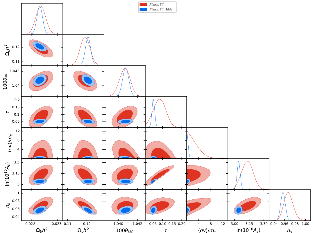
Fig.3 visualizes the correlation between DM annihilation injection (parameterized by $\left<\sigma v\right>/m_{\chi}$) and the base $\Lambda$CDM cosmological parameters. The constraints are obtained by fitting Planck 2018 TT (red) and TT+TE+EE (blue) data with the CosmoMC codes Lewis and Bridle 2002; Lewis 2013. Tilting in the elliptical contour’s axis indicate parameter correlation. The resulting linear correlation coefficients between $\left<\sigma v\right>/m_{\chi}$ and six relevant cosmological parameters are listed in Tab. I. With the inclusion of polarization we observe a significant reduction of parameter degeneracies.

DM clustering boost has a huge impact on $x_{\rm{e}}$ and $T_{\rm IGM}$ at late time. However, because CMB is rather insensitive to energy injection at low redshift, the changes to the anisotropy spectra are relatively minor, as demonstrated most evidently in TT and EE panels in Fig. 2.

	TT	TT,TE,EE
$\tau$	-0.22	-0.04
$n_{\rm s}$	0.59	0.14
$\ln(10^{10}A_{\rm s})$	0.17	0.27
$\Omega_{\rm b}h^{2}$	0.17	0.07
$\Omega_{\rm c}h^{2}$	-0.08	0.16
$100\theta_{\rm MC}$	-0.37	-0.28

Table 1: Linear correlation coefficients between $\left<\sigma v\right>/m_{\chi}$ and cosmological parameters corresponding to Fig.3.

IV Sensitivity Estimates

Several upcoming observations are expected to conduct high precision measurement of CMB polarization anisotropy at $\mu{\rm{K}}$-${\rm{arcmin}}$ sensitivities with arcmin beams, including AdvACTPol Calabrese et al. 2014; Li et al. 2018a, AliCPT Li et al. 2018b; Li et al. 2017, CLASS Essinger-Hileman et al. 2014, LiteBird Hazumi et al. 2019, Simons Array Suzuki et al. 2016; Arnold et al. 2014, Simons Observatory Ade et al. 2019, SPT-3G  Anderson et al. 2018, and many more proposed for the future Abazajian et al. 2016; Alvarez et al. 2019; Calabrese et al. 2017; Di Valentino et al. 2018. We will study the expected sensitivities on DM injection of a few missions that are either already operational or will be so in near future.

IV.1 Forecasting Procedure

Assuming null signal, a sensitivity bound on DM energy injection can be placed by testing the spectral deviation from fiducial TT, TE and EE anisotropy spectra $\hat{C_{\ell}}$ that serve as fake data. We use the “exact full sky” likelihood function Hamimeche and Lewis 2008 for significance calculation,

$$-2{\ln}\mathcal{L}(\{C_{\ell}\}|\{{\hat{C}_{\ell}}\})=\ \ \ \ \ \ \ \ \ \ \ \$$ (21)

$$f_{\rm sky}\times\sum_{\ell}(2\ell+1)\{{\rm{Tr}}[{\hat{C}_{\ell}}C_{\ell}^{-1}] - {\ln}|{\hat{C}_{\ell}}C_{\ell}^{-1}|-2\}$$

where $f_{\rm{sky}}$ is the fraction of sky covered by an experiment, $C_{\ell}$ is a function of cosmological and DM parameters, while $\hat{C_{\ell}}$ is a simulated anisotropy spectra serving as mocked data. With both temperature (T) and polarization (E) correlations, $C_{\ell}$ and $\hat{C_{\ell}}$ are $2\times 2$ matrices:

$$C_{\ell}\equiv\begin{bmatrix}C_{\ell}^{TT}&C_{\ell}^{TE}\\ C_{\ell}^{TE}&C_{\ell}^{EE}\\ \end{bmatrix}$$ (22)

$$\hat{C}_{\ell}\equiv\begin{bmatrix}\bar{C}_{\ell}^{TT}+N_{\ell}^{TT}&\bar{C}_{\ell}^{TE}\\ \bar{C}_{\ell}^{TE}&\bar{C}_{\ell}^{EE}+N_{\ell}^{EE}\\ \end{bmatrix}$$ (23)

The fixed ‘fiducial’ $\bar{C}_{\ell}$ is generated using Planck 2018 best-fit  Aghanim et al. 2018 $\Lambda$CDM parameters ($\Omega_{\rm{b}}h^{2}=0.0224$, $\Omega_{\rm{c}}h^{2}=0.1193$, $100\theta_{{\rm{MC}}}=1.041$, $\tau=0.056$, $\ln(10^{10}A_{\rm{s}})=3.047$, $n_{\rm{s}}=0.967$), without DM injection. $N_{\ell}^{TT}$ and $N_{\ell}^{EE}$ are the instrumental white noise power spectra, for a multi-frequency CMB experiment they are given by Knox 1995; Errard et al. 2016:

$$N^{{\rm{EE}}}_{\ell} = \left[\sum_{\nu}\omega_{E,\nu}{\exp}\left(-\ell(\ell+1)\frac{\theta^{2}_{\rm{FWHM},\nu}}{8\ {\ln}2}\right)\right]^{-1}$$ (24)

$$N^{{\rm{TT}}}_{\ell} = \frac{1}{2}\ N^{{\rm{EE}}}_{\ell}$$ (25)

here the subscript $\nu$ labels the frequency channel, $\omega_{{\rm{E}},\nu}^{-\frac{1}{2}}$ is the white noise level in $\mu{\rm{k}}\cdot{\rm{rad}}$. $\theta_{\rm{FWHM},\nu}$ denotes the full width at half maximum beam size in radians. Specifications for experiments considered are collected in Appendix A.

In addition to detector noises, residual foreground would be a contamination that contributes to $\hat{C}_{\ell}$. However it is beyond the scope of this paper to make robust foreground removal estimate for each experiment, and we present the results assuming the anisotropy foreground has been successfully subtracted.

IV.2 Prospective limits

Here we present the prospective limits of DM annihilation and decay rates. Both $m_{\chi}^{-1}\left<\sigma v\right>$ and $\Gamma_{\chi}$ are considered time and velocity independent. The dark matter parameters $m_{\chi}$, $m_{\chi}^{-1}\left<\sigma v\right>$ and $\Gamma_{\chi}$ are included into CosmoMC as new variables. We marginalize over $\Lambda$CDM parameters to derive the bounds on dark matter papers. Experimental nuisance parameters are also marginalized over in case Planck data are included. CosmoMC uses a preset Gelman-Rubin “mean of chain variance” $R$ value as the convergence criterion in the Markov chain process, and we ensure $R-1\leq$ 0.01 in the results.

First we analyze the limit with Planck 2018 Aghanim et al. 2019 and Baryon Acoustic Oscillations (BAO) Alam et al. 2017; Beutler et al. 2011; Ross et al. 2015 data as a cross-check and a benchmark. The Planck likelihoods used are: (i) the high-$\ell$ TTTEEE plike likelihood, (ii) low-$\ell$ TT and EE likelihoods, (iii) lensing likelihood. As shown in Fig. 4, our 95% C.L. limits for annihilation (red dotted curves) are in good agreement with Ref. Aghanim et al. 2018 (We also found good consistency with the results in Ref. Slatyer and Wu 2017 and Liu et al. 2016 using Planck 2015 data). The 21 nuisance parameters in Planck likelihoods are also varied in the fitting process and marginalized over in our results. Constraints on $\Gamma_{\chi}$ for a characteristic WIMP mass of $m_{\chi}=10{\rm{GeV}}$ are collected in Tabs.2. Lower bounds on $m_{\chi}$ (assuming a thermal cross section) are shown in Tab.3.

Compared with current Planck limits, upcoming experiments yield either comparable or significantly improved bounds. When the limits are close to Planck bounds, it benefits from a joint analysis. For instance AliCPT sensitivity improves by around 30% if combined with Planck data. Projected limits for AdvACTPol, SPT-3G and Simons Observatory extend to $\left<\sigma v\right>/m_{\chi}\sim\rm{10^{-28}cm^{3}s^{-1}GeV^{-1}}$ and $\Gamma_{\chi}\sim\rm{10^{-26}}s^{-1}$. Simons Array is estimated to be sensitive to $\left<\sigma v\right>/m_{\chi}\sim\rm{10^{-29}cm^{3}s^{-1}GeV^{-1}}$ and $\Gamma_{\chi}\sim\rm{10^{-27}}{~\rm{s^{-1}}}$. We also found that BICEP2/KECK Array 2018 Ade et al. 2018 places 95% C.L. upper bounds at $\left<\sigma v\right>/m_{\chi}\sim 10^{-26}{\rm{cm^{3}s^{-1}GeV^{-1}}}$ and $\Gamma_{\chi}\sim 10^{-23}s^{-1}$, which are less stringent than Planck.

DM mass-dependence in the shape of sensitivity bounds reflects the energy deposit efficiency’s dependence on the injection energy. The constraints are much tighter around $10$-$100$ MeV DM mass. The reason is that electrons and photons injected at this energy range can produce photons with energies $10$ eV-$1$ KeV by either up-scattering on CMB photons or Compton scattering on electrons, which efficiently ionize hydrogen atomsSlatyer and Wu 2017.

The illustrated annihilation constraints assume clustering enhancements except for a comparison case (mid and lower panels, red dotted), for which we show a Planck bounds with a homogeneous DM distribution. The polarization anisotropy is expected to be more sensitive to higher redshift injection, around $z=600\sim 1000$ Finkbeiner et al. 2012; Contaldi 2016, and the late time injection may become obscured by the uncertainty in reionization history. We found that our constraints on annihilating DM are mostly unaffected by DM clustering effect. For Planck data, inclusion of clustering enhancement gives only a slight 2% difference in the annihilation cross-section bound. Given the significant $x_{\rm{e}}$ and $T_{\rm IGM}$ increase at low redshift, future precision measurement on the reionization epoch may improve this situation.

Figure 4: Limits on DM decay (top panels, $\left<\sigma v\right>/m_{\chi}=0$) and annihilation (middle and bottom panels, $\Gamma_{\chi}=0$) parameters. Regions above the lines are excluded at 95% confidence level. All annihilation constraints assume the case with DM clustering unless labeled otherwise. Constraints labeled $Planck$ are obtained by fitting $Planck2018$ Aghanim et al. 2019 + BAO Alam et al. 2017; Beutler et al. 2011; Ross et al. 2015 datasets. Left and right panels correspond to $e^{-}e^{+}$ and $\gamma\gamma$ final states respectively. The bottom panels show the constraints in $\left<\sigma v\right>$ - ${m_{\chi}}$ plane corresponding to the $\left<\sigma v\right>/{m_{\chi}}$ - ${m_{\chi}}$ constraints in middle panels. Planck constraints on annihilation in unclustered (homogeneous) DM distribution model are also shown in red dotted lines for comparison. The legend applies to all panels. $\Lambda$CDM parameters and $Planck$’s nuisance parameters are marginalized over.

Experiment	$\chi\to e^{+}e^{-}$	$\chi\to\gamma\gamma$
Planck	$24$	$85$
AdvACTPol	$0.68$	$4.7$
AliCPT	$21$	$78$
AliCPT+Planck	$16$	$53$
CLASS	$5.5$	$30$
Simons Array	$0.35$	$1.5$
Simons Observatory	$0.92$	$4.2$
SPT-3G	$2.2$	$9.9$

Table 2: Expected 95% C.L. upper limit on $\Gamma_{\chi}$ (in $10^{-26}{~\rm{s^{-1}}}$) at $m_{\chi}=10$ GeV.

Experiment	$\chi\chi\to e^{+}e^{-}$	$\chi\chi\to\gamma\gamma$
Planck	$39$	$32$
Planck - Unclustered	$39$	$33$
AdvACTPol	$330$	$330$
AliCPT	$32$	$22$
AliCPT+Planck	$51$	$42$
CLASS	$49$	$37$
Simons Array	$1.1\times 10^{3}$	$1.0\times 10^{3}$
Simons Observatory	$310$	$290$
SPT-3G	$140$	$130$

Table 3: Expected 95% C.L. lower limit on $m_{\chi}$ (in $\rm{GeV}$) assuming a thermal relic’s annihilation cross-section $\left<\sigma v\right>=3\times 10^{-26}{~\rm{cm^{3}/s}}$.

V Conclusion

WIMP dark matter decay and annihilation during the cosmic dark ages can inject high-energy particles into the intergalactic medium, which then heats and ionized the neutral gas. This effect widens the last scattering surface, attenuating polarization and temperature fluctuation on small scales while shifting peak locations of polarization anisotropy spectra.

In this paper, we made DM sensitivity forecast for several upcoming CMB experiments in detecting dark matter in 10 KeV - 10 TeV mass range that decay or annihilate into $e^{-}e^{+}$/$\gamma\gamma$. These experiments are either already operational or undergoing construction, including AdvACTPol, AliCPT, CLASS, Simons Array, Simons Observatory and SPT-3G. Assuming complete foreground removal, we found that these instruments are capable of significantly improving current CMB constraints on DM decay lifetime and annihilation cross section set by Planck satellite, with Simons Array giving 95% CL upper bounds of $\left<\sigma v\right>/m_{\chi}\sim 10^{-29}{~\rm{cm}}^{3}{\rm{s}}^{-1}{\rm{GeV}}^{-1}$ for annihilation and $\Gamma_{\chi}\sim 10^{-27}{\rm{s}}^{-1}$ for decay, nearly two orders of magnitudes more stringent than Planck bounds. Assuming a thermal relic cross-section ($\left<\sigma v\right>\ =3\times 10^{-26}{~\rm{cm^{3}s^{-1}}}$), annihilation constraints from Simons Array can be translated into DM mass lower bounds of $m_{\chi}>1.06\rm{TeV}$ for $e^{-}e^{+}$ channel, and $m_{\chi}>1.01\rm{TeV}$ for $\gamma\gamma$ channel. These limits span over a wide range of DM mass that fills the energy gap in indirect cosmic X-ray and $\gamma$-ray searches and further tightens the lower bounds on the mass of thermally produced dark matter.

DM injection induces distinctly different patterns of deviation in temperature and polarization anisotropy spectra, which helps to break the degeneracy between DM and cosmological parameters. Promising limits on dark matter annihilation and decay rates can be expected at upcoming CMB experiments. In the case of DM annihilation, DM clustering at low redshift can have dramatic impacts on ionization fraction and IGM temperature. However, its effect on the CMB anisotropy is less prominent due to uncertainties in astrophysical injection during the reionization epoch. Future high precision CMB and 21cm experiments can significantly improve the sensitivity to DM clustering.

Acknowledgements

We thank Shulei Ni, Siyu Li, Hong Li, Xiaojun Bi and Steven Clark for helpful discussions, and Tracy R. Slatyer, Hongwan Liu for updated deposition efficiency data. Y.G. is supported by the Institute of High Energy Physics, Chinese Academy of Sciences under grant no. Y7515560U1. Y.Z.M. acknowledges the supports from National Research Foundation with grant no. 105925, 109577, 120378, and 120385, and National Science Foundation China with grant no. 11828301.

Appendix A Experimental Specifications

${\rm{Experiment}}$	$\ \ \ \nu{\rm{[GHz]}}\ \ \$	$\ \ \ \omega_{{\rm{E}},\nu}^{-1/2}\ [\mu{\rm{K}}$-${\rm{arcmin}}]\ \ \$	$\ \ \ \theta_{\rm{FWHM}}[\rm{arcmin}]\ \ \$	$\ \ \ f_{\rm{sky}}[\%]\ \ \$	$\ \ \ \ell_{\rm{min}}\ \ \$	$\ \ \ \ell_{\rm{max}}\ \ \$
AdvACTPol  Calabrese et al. 2014; Henderson et al. 2016; Aiola et al. 2020	28	113.1	7.1	50	350	4000
	41	99.0	4.8
	90 $\star$	11.3	2.2
	150 $\star$	9.9	1.4
	230	35.4	0.9
AliCPT Li et al. 2019	90$\star$	2	15.4	10	30	600
	150$\star$	2	9.7
CLASS Essinger-Hileman et al. 2014	38	39	90	70	5	200
	93$\star$	13	40
	148$\star$	15	24
	217	43	18
Simons Array Arnold et al. 2014; Creminelli et al. 2015	95$\star$	13.9	5.2	65	30	3000
	150$\star$	11.4	3.5
	220	30.1	2.7
Simons Observatory - SAT Ade et al. 2019	27	35.4	93	10	25	1000
	39	24	63
	93$\star$	2.7	30
	145$\star$	3	17
	225	6	11
	280	14.1	9
Simons Observatory - LAT Ade et al. 2019	27	73.5	7.4	40	1000	5000
	39	38.2	5.1
	93$\star$	8.2	2.2
	145$\star$	8.9	1.4
	225	21.2	1
	280	52.3	0.9
SPT-3G Benson et al. 2014; Anderson et al. 2018; Creminelli et al. 2015	95$\star$	5.1	1	6	50	5000
	150$\star$	4.7	1
	220	12.0	1

Table 4: Specifications for experiments considered in this work. Note that we only use frequency channels in $90\sim 150{~\rm{GHz}}$ (labeled with $\star$) range, other frequencies are usually more purposed for monitoring foregrounds and are therefore not included in our forecast.

References

- Cushman et al. (2013) P. Cushman et al., in Community Summer Study 2013 (2013) arXiv:1310.8327 [hep-ex] .
- Profumo (2013) S. Profumo (2013) pp. 143–189, arXiv:1301.0952 [hep-ph] .
- Boveia and Doglioni (2018) A. Boveia and C. Doglioni, Ann. Rev. Nucl. Part. Sci. 68, 429 (2018), arXiv:1810.12238 [hep-ex] .
- Schumann (2019) M. Schumann, J. Phys. G46, 103003 (2019), arXiv:1903.03026 [astro-ph.CO] .
- Chen and Kamionkowski (2004) X.-L. Chen and M. Kamionkowski, Phys. Rev. D70, 043502 (2004), arXiv:astro-ph/0310473 [astro-ph] .
- Adams et al. (1998) J. A. Adams, S. Sarkar, and D. Sciama, Mon. Not. Roy. Astron. Soc. 301, 210 (1998), arXiv:astro-ph/9805108 .
- Padmanabhan and Finkbeiner (2005) N. Padmanabhan and D. P. Finkbeiner, Phys. Rev. D72, 023508 (2005), arXiv:astro-ph/0503486 [astro-ph] .
- Pierpaoli (2004) E. Pierpaoli, Phys. Rev. Lett. 92, 031301 (2004), arXiv:astro-ph/0310375 [astro-ph] .
- Acharya and Khatri (2019) S. K. Acharya and R. Khatri, (2019), arXiv:1910.06272 [astro-ph.CO] .
- Aghanim et al. (2018) N. Aghanim et al. (Planck), (2018), arXiv:1807.06209 [astro-ph.CO] .
- Slatyer and Wu (2017) T. R. Slatyer and C.-L. Wu, Phys. Rev. D95, 023010 (2017), arXiv:1610.06933 [astro-ph.CO] .
- Slatyer (2016a) T. R. Slatyer, Phys. Rev. D93, 023527 (2016a), arXiv:1506.03811 [hep-ph] .
- Liu et al. (2016) H. Liu, T. R. Slatyer, and J. Zavala, Phys. Rev. D94, 063507 (2016), arXiv:1604.02457 [astro-ph.CO] .
- Kawasaki et al. (2016) M. Kawasaki, K. Nakayama, and T. Sekiguchi, Phys. Lett. B756, 212 (2016), arXiv:1512.08015 [astro-ph.CO] .
- Aghanim et al. (2019) N. Aghanim et al. (Planck), (2019), arXiv:1907.12875 [astro-ph.CO] .
- Aghanim et al. (2016) N. Aghanim et al. (Planck), Astron. Astrophys. 594, A11 (2016), arXiv:1507.02704 [astro-ph.CO] .
- Ahnen et al. (2016) M. L. Ahnen et al. (MAGIC, Fermi-LAT), JCAP 1602, 039 (2016), arXiv:1601.06590 [astro-ph.HE] .
- Grayson et al. (2016) J. A. Grayson et al. (BICEP3), Proc. SPIE Int. Soc. Opt. Eng. 9914, 99140S (2016), arXiv:1607.04668 [astro-ph.IM] .
- Anderson et al. (2018) A. J. Anderson et al. (SPT), J. Low. Temp. Phys. 193, 1057 (2018).
- Calabrese et al. (2014) E. Calabrese et al., JCAP 1408, 010 (2014), arXiv:1406.4794 [astro-ph.CO] .
- Li et al. (2018a) Y. Li et al., Proc. SPIE Int. Soc. Opt. Eng. 10708, 107080A (2018a).
- Essinger-Hileman et al. (2014) T. Essinger-Hileman et al., Proc. SPIE Int. Soc. Opt. Eng. 9153, 91531I (2014), arXiv:1408.4788 [astro-ph.IM] .
- Suzuki et al. (2016) A. Suzuki et al. (POLARBEAR), J. Low. Temp. Phys. 184, 805 (2016), arXiv:1512.07299 [astro-ph.IM] .
- Arnold et al. (2014) K. Arnold et al., Proc. SPIE Int. Soc. Opt. Eng. 9153, 91531F (2014).
- Ade et al. (2019) P. Ade et al. (Simons Observatory), JCAP 1902, 056 (2019), arXiv:1808.07445 [astro-ph.CO] .
- Li et al. (2017) Y.-P. Li, Y. Liu, S.-Y. Li, H. Li, and X. Zhang, (2017), arXiv:1709.09053 [astro-ph.IM] .
- Weniger et al. (2013) C. Weniger, P. D. Serpico, F. Iocco, and G. Bertone, Phys. Rev. D87, 123008 (2013), arXiv:1303.0942 [astro-ph.CO] .
- Slatyer et al. (2009) T. R. Slatyer, N. Padmanabhan, and D. P. Finkbeiner, Phys. Rev. D80, 043526 (2009), arXiv:0906.1197 [astro-ph.CO] .
- Slatyer (2013) T. R. Slatyer, Phys. Rev. D87, 123513 (2013), arXiv:1211.0283 [astro-ph.CO] .
- Belotsky and Kirillov (2015) K. M. Belotsky and A. A. Kirillov, JCAP 1501, 041 (2015), arXiv:1409.8601 [astro-ph.CO] .
- Liu et al. (2019) H. Liu, G. W. Ridgway, and T. R. Slatyer, (2019), arXiv:1904.09296 [astro-ph.CO] .
- Shull and van Steenberg (1985) J. M. Shull and M. E. van Steenberg, Astrophys. J. 298, 268 (1985).
- Slatyer (2016b) T. R. Slatyer, Phys. Rev. D93, 023521 (2016b), arXiv:1506.03812 [astro-ph.CO] .
- Taylor and Silk (2003) J. E. Taylor and J. Silk, Mon. Not. Roy. Astron. Soc. 339, 505 (2003), arXiv:astro-ph/0207299 [astro-ph] .
- Schneider et al. (2013) A. Schneider, R. E. Smith, and D. Reed, Mon. Not. Roy. Astron. Soc. 433, 1573 (2013), arXiv:1303.0839 [astro-ph.CO] .
- Sheth and Tormen (1999) R. K. Sheth and G. Tormen, Mon. Not. Roy. Astron. Soc. 308, 119 (1999), arXiv:astro-ph/9901122 [astro-ph] .
- Einasto (1965) J. Einasto, Trudy Astrofizicheskogo Instituta Alma-Ata 5, 87 (1965).
- Klypin et al. (2016) A. Klypin, G. Yepes, S. Gottlober, F. Prada, and S. Hess, Mon. Not. Roy. Astron. Soc. 457, 4340 (2016), arXiv:1411.4001 [astro-ph.CO] .
- Ali-Haimoud and Hirata (2011) Y. Ali-Haimoud and C. M. Hirata, Phys. Rev. D83, 043513 (2011), arXiv:1011.3758 [astro-ph.CO] .
- Lewis et al. (2000) A. Lewis, A. Challinor, and A. Lasenby, Astrophys. J. 538, 473 (2000), arXiv:astro-ph/9911177 [astro-ph] .
- Lewis and Bridle (2002) A. Lewis and S. Bridle, Phys. Rev. D66, 103511 (2002), arXiv:astro-ph/0205436 [astro-ph] .
- Lewis (2013) A. Lewis, Phys. Rev. D87, 103529 (2013), arXiv:1304.4473 [astro-ph.CO] .
- Li et al. (2018b) H. Li, S.-Y. Li, Y. Liu, Y.-P. Li, and X. Zhang, Nat. Astron. 2, 104 (2018b), arXiv:1802.08455 [astro-ph.IM] .
- Hazumi et al. (2019) M. Hazumi et al., J. Low. Temp. Phys. 194, 443 (2019).
- Abazajian et al. (2016) K. N. Abazajian et al. (CMB-S4), (2016), arXiv:1610.02743 [astro-ph.CO] .
- Alvarez et al. (2019) M. Alvarez et al., (2019), arXiv:1908.07495 [astro-ph.IM] .
- Calabrese et al. (2017) E. Calabrese, D. Alonso, and J. Dunkley, Phys. Rev. D95, 063504 (2017), arXiv:1611.10269 [astro-ph.CO] .
- Di Valentino et al. (2018) E. Di Valentino et al. (CORE), JCAP 1804, 017 (2018), arXiv:1612.00021 [astro-ph.CO] .
- Hamimeche and Lewis (2008) S. Hamimeche and A. Lewis, Phys. Rev. D77, 103013 (2008), arXiv:0801.0554 [astro-ph] .
- Knox (1995) L. Knox, Phys. Rev. D52, 4307 (1995), arXiv:astro-ph/9504054 [astro-ph] .
- Errard et al. (2016) J. Errard, S. M. Feeney, H. V. Peiris, and A. H. Jaffe, JCAP 1603, 052 (2016), arXiv:1509.06770 [astro-ph.CO] .
- Alam et al. (2017) S. Alam et al. (BOSS), Mon. Not. Roy. Astron. Soc. 470, 2617 (2017), arXiv:1607.03155 [astro-ph.CO] .
- Beutler et al. (2011) F. Beutler, C. Blake, M. Colless, D. H. Jones, L. Staveley-Smith, L. Campbell, Q. Parker, W. Saunders, and F. Watson, Mon. Not. Roy. Astron. Soc. 416, 3017 (2011), arXiv:1106.3366 [astro-ph.CO] .
- Ross et al. (2015) A. J. Ross, L. Samushia, C. Howlett, W. J. Percival, A. Burden, and M. Manera, Mon. Not. Roy. Astron. Soc. 449, 835 (2015), arXiv:1409.3242 [astro-ph.CO] .
- Ade et al. (2018) P. A. R. Ade et al. (BICEP2, Keck Array), Phys. Rev. Lett. 121, 221301 (2018), arXiv:1810.05216 [astro-ph.CO] .
- Finkbeiner et al. (2012) D. P. Finkbeiner, S. Galli, T. Lin, and T. R. Slatyer, Phys. Rev. D85, 043522 (2012), arXiv:1109.6322 [astro-ph.CO] .
- Contaldi (2016) C. R. Contaldi, Int. J. Mod. Phys. D25, 1640014 (2016).
- Henderson et al. (2016) S. Henderson et al., J. Low Temp. Phys. 184, 772 (2016), arXiv:1510.02809 [astro-ph.IM] .
- Aiola et al. (2020) S. Aiola et al. (ACT), (2020), arXiv:2007.07288 [astro-ph.CO] .
- Li et al. (2019) H. Li et al., Natl. Sci. Rev. 6, 145 (2019), arXiv:1710.03047 [astro-ph.CO] .
- Creminelli et al. (2015) P. Creminelli, D. L. López Nacir, M. Simonović, G. Trevisan, and M. Zaldarriaga, JCAP 1511, 031 (2015), arXiv:1502.01983 [astro-ph.CO] .
- Benson et al. (2014) B. Benson et al. (SPT-3G), Proc. SPIE Int. Soc. Opt. Eng. 9153, 91531P (2014), arXiv:1407.2973 [astro-ph.IM] .