Proper Learning of Linear Dynamical Systems as a Non-Commutative Polynomial optimization Problem

Abstract

There has been much recent progress in forecasting the next observation of a linear dynamical system (LDS), which is known as the improper learning, as well as in the estimation of its system matrices, which is known as the proper learning of LDS. We present an approach to proper learning of LDS, which in spite of the non-convexity of the problem, guarantees global convergence of numerical solutions to a least-squares estimator. We present promising computational results.

1 Introduction

We consider the identification of vector autoregressive processes with hidden components from time series of observations. This problem is also known as proper learning of linear dynamical systems (LDS), and provides a very general approach to time-series analysis. Its applications range from learning population-growth models in actuarial science and mathematical biology Leslie (1945) to functional analysis in neuroscience Besserve et al. (2010). Indeed, one encounters either partially observable processes Åström (1965) or questions of causality Pearl (2009) that can be tied to proper learning of LSD Geiger et al. (2015) in almost any application domain.

To state the problem formally, let us define an observable linear system $L=(G,F,\nu,W)$ as in West & Harrison (1997):

$$\phi_{t} = G\phi_{t-1}+\omega_{t},$$

$$Y_{t} = F^{\prime}\phi_{t}+\nu_{t},$$

where $\phi_{t}\in\mathbb{R}^{n}$ is the hidden state, $Y_{t}\in\mathbb{R}^{m}$ is the observed output of $L$ (measurements, observations), $G\in\mathbb{R}^{n\times n}$ and $F\in\mathbb{R}^{n\times m}$ are system matrices, and $\{\omega_{t},\nu_{t}\}_{t=1}^{\infty}$ are process and observation noises. Proper learning refers to identifying the quadruple $(G,F,\nu,W)$ given the output $\{Y_{t}\}_{t\in\mathbb{N}}$ of $L$. This also allows for the estimation of subsequent observations, which is known as the “prediction-error” approach to improper learning Ljung (1998). There are two complications. First, the corresponding optimization problem is non-convex, and guarantees of global convergence have consequently been available only for certain special cases so far. Second, the dimension $n$ of the hidden state $\phi_{t}$ is not known, in general. Although Sarkar et al. (2019) have shown that a lower-dimensional model can approximate a higher-dimensional one rather well, in many cases, it is hard to pick $n$ in practice.

Our goal is to develop a method for proper learning of LDS that could also estimate the dimension of the hidden state and that would do so with guarantees of global convergence to the best possible estimate, given the observations.

1.1 Motivation

While there are numerous important applications involving non-trivial hidden components Åström (1965); Pearl (2009); Besserve et al. (2010); Geiger et al. (2015), let us illustrate the importance of the identification of system matrices on a simple example of the age-structured matrix model in actuarial science and mathematical biology Leslie (1945). There, the growth of the population has the form:

$$N_{t+1}=AN_{t},$$ (1)

where $N_{t}$ and $N_{t+1}$ are the vectors of abundance at time $t$ and $t+1$ respectively. To be more specific, if we divide a species into $n$ age classes according to their life cycles, there will be $n$ elements in the vector $N_{t}$, denoted by $N_{t}^{(1)},N_{t}^{(2)},\dots,N_{t}^{(n)}$, where $N_{t}^{(i)}$ is defined to be the number of individuals in the $i^{th}$ age class. $A\in\mathbb{R}^{n\times n}$ is the transition matrix. Since $N_{t}$ and $N_{t+1}$ have a linear relation, it is obvious that (1) is a linear dynamical system.

$${\left[\begin{array}[]{c}N_{t+1}^{(1)}\\ N_{t+1}^{(2)}\\ \cdots\\ N_{t+1}^{(n-1)}\\ N_{t+1}^{(n)}\end{array}\right]}={\left[\begin{array}[]{ccccc}F_{1}&F_{2}&\cdots&F_{n-1}&F_{n}\\ P_{1,2}&P_{2,2}&\cdots&0&0\\ \cdots&\cdots&\cdots&\cdots&\cdots\\ 0&0&\cdots&P_{n-1,n-1}&0\\ 0&0&\cdots&P_{n-1,n}&P_{n,n}\end{array}\right]}{\left[\begin{array}[]{c}N_{t}^{(1)}\\ N_{t}^{(2)}\\ \cdots\\ N_{t}^{(n-1)}\\ N_{t}^{(n)}\end{array}\right]},$$

Figure 1: An illustration of the age-structured matrix model Leslie (1945), where $P_{i,j}$ $j\geq i\in[1,2,\dots,n]$, is the probability of an individual at the $i^{th}$ age class surviving to the $j^{th}$ age class. $F_{i},i\in[1,2,\dots,n]$ is the fecundity of the the $i^{th}$ age class, i.e., the product of birth rate and surviving probability.

Assuming the first age class is pre-reproductive and the rest are reproductive, the age-structured matrix model in (1) can be rewritten in a matrix notation, as illustrated in Figure 1. With this illustration in mind, the benefits of proper learning are clear:

• Discovery of the actual dynamics: while the abundance vector $N_{t}$ can also be estimated using improper learning, the surviving probabilities and fecundity of each age class can be obtained using proper learning.

• Usage of prior information or shape constraints: proper learning makes it possible to use problem-specific information in constraints on the decision variables. In the age-structured model, for example, we know some enties of $A$ are zeros, e.g., first age group are immature ($F_{1}=0$). Generally, we know the sequence of $F_{i}$ without $F_{1}$ should be monotonically decreasing, because the individuals are getting older. While one may develop improper learning specific to a given shape constraint Rosenfeld et al. (2020) in an ad hoc fashion, proper learning makes this easier.

• Explainability: unlike many other forecasting methods, proper learning makes it easy to explain “why”.

• Robustness: The learned model can be compared with prior information to check for consistency. In many applications, the measurement chain has guarantees on the overall error. One can hence translate such guarantees to a bound on the magnitude of the measurement noise from above.

1.2 Contributions

Our contributions are:

• We cast proper learning of a linear dynamical system as a non-commutative polynomial optimization problem (NCPOP), in several ways.

• We show how to use prior information as constraints in the NCPOP.

• We study the numerical methods for solving the resulting NCPOP and extracting its optimizer. In simple numerical examples studied previously, it outperforms standard subspace and least-squares methods.

2 Background

In Section 2.1, we set our work in the context of related work. In Section 2.2, we provide a brief overview of non-commutative polynomial optimization, pioneered by Pironio et al. (2010) and nicely surveyed by Burgdorf et al. (2016), which is our key technical tool. Prior to introducing our own results, we introduce some common notation in Section 2.3, following West & Harrison (1997) and Kozdoba et al. (2019).

2.1 Related Work in System Identification and Control

Research within System Identification variously appears in venues associated with Control Theory, Statistics, and Machine learning. We refer to Ljung (1998) and Tangirala (2014) for excellent overviews of the long history of research in the field, going back at least to Åström & Torsten (1965). In this section, we focus on pointers to key more recent publications.

In improper learning of LDS, a considerable progress has been made in the analysis of predictions for the expectation of the next measurement using auto-regressive (AR) processes. In Anava et al. (2013), first guarantees were presented for auto-regressive moving-average (ARMA) processes. In Liu et al. (2016), these results were extended to a subset of autoregressive integrated moving average (ARIMA) processes. Kozdoba et al. (2019) have shown that up to an arbitrarily small error given in advance, AR($s$) will perform as well as any Kalman filter on any bounded sequence. This has been extended by Tsiamis & Pappas (2020) to Kalman filtering with logarithmic regret. Another stream of work within improper learning focuses on sub-space methods Katayama (2006); Van Overschee & De Moor (1996) and spectral methods. Tsiamis et al. (2019); Tsiamis & Pappas (2019) presented the present-best guarantees for traditional sub-space methods. Within spectral methods, Hazan et al. (2017) and Hazan et al. (2018) have considered learning LDS with input, employing certain eigenvalue-decay estimates of Hankel matrices in the analyses of an auto-regressive process in a dimension increasing over time. We stress that none of these approaches to improper learning are “prediction-error”: They do not estimate the system matrices.

In proper learning of LDS, many state-of-the-art approaches consider the least-squares method, despite complications encountered in unstable systems Faradonbeh et al. (2018). Simchowitz et al. (2018) have provided non-trivial guarantees for the ordinary least-squares (OLS) estimator in the case of stable $G$ and there being no hidden component, i.e., $F^{\prime}$ being an identity and $Y_{t}=\phi_{t}$. Surprisingly, they have also shown that more unstable linear systems are easier to estimate than less unstable ones, in some sense. Simchowitz et al. (2019) extended the results to allow for a certain pre-filtering procedure. Sarkar & Rakhlin (2019) extended the results to cover stable, marginally stable, and explosive regimes. Our work could be seen as a continuation of the least squares method to processes with hidden components, with guarantees of global convergence. In Computer Science, our work could be seen as an approximation scheme Vazirani (2013), as it allows for $\epsilon$ error for any $\epsilon>0$.

2.2 Non-Commutative Polynomial Optimization

Our key technical tool is non-commutative polynomial optimization (NCPOP), first introduced by Pironio et al. (2010). Here, we provide a brief sumary of their results, and refer to Burgdorf et al. (2016) for a book-length introduction. NCPOP is an operator-valued optimization problem with a standard form in 2:

$$P:\begin{aligned} p*=~&\underset{\displaystyle(H,X,\phi)}{\mathrm{min}}\quad\langle\phi,p(X)\phi\rangle\hfil\hfil\displaystyle\displaystyle\hfil\hfil\displaystyle\displaystyle\\ &\mathmakebox[\widthof{$\underset{\displaystyle\phantom{(H,X,\phi)}}{\mathrm{min}}$}][c]{\mathmakebox[\widthof{$\mathrm{min}$}][l]{\mathrm{\kern 1.00006pts.t.}}}\quad&q_{i}(X)&\succcurlyeq 0,&&i=1,\ldots,m,\\ &\quad&\langle\phi,\phi\rangle&=1,\end{aligned}$$ (2)

where $X=(X_{1},\ldots,X_{n})$ is a bounded operator on a Hilbert space $\mathcal{H}$. The normalized vector $\phi$, i.e., $\|\phi\|^{2}=1$ is also defined on $\mathcal{H}$ with inner product $\langle\phi,\phi\rangle$ equals to $1$. $p(X)$ and $q_{i}(X)$ are polynomials and $q_{i}(X)\succcurlyeq 0$ denotes that the operator $q_{i}(X)$ is positive semi-definite. Polynomials $p(X)$ and $q_{i}(X)$ of degrees $\deg(p)$ and $\deg(q_{i})$, respectively, can be written as:

$$p(X)=\sum_{|\omega|\leq\deg(p)}p_{\omega}\omega,\quad q_{i}(X)=\sum_{|\mu|\leq\deg(q_{i})}q_{i,\mu}\mu,$$ (3)

where $i=1,\ldots,m$. Following Akhiezer & Krein (1962), we can define the moments on field $\mathbb{R}$ or $\mathbb{C}$, with a feasible solution $(H,X,\phi)$ of problem (2):

$$y_{\omega}=\langle\phi,\omega(X)\phi\rangle,$$ (4)

for all $\omega\in\mathcal{W}_{\infty}$ and $y_{1}=\langle\phi,\phi\rangle=1$. Given a degree $k$, the moments whose degrees are less or equal to $k$ form a sequence of $y=(y_{\omega})_{|\omega|\leq 2k}$. With a finite set of moments $y$ of degree $k$, we can define a corresponding $k^{th}$ order moment matrix $M_{k}(y)$:

$$M_{k}(y)(\nu,\omega)=y_{\nu^{{\dagger}}\omega}=\langle\phi,\nu^{{\dagger}}(X)\omega(X)\phi\rangle,$$ (5)

for any $|\nu|,|\omega|\leq k$ and a localizing matrix $M_{k-d_{i}}(q_{i}y)$:

$$M_{k-d_{i}}(q_{i}y)(\nu,\omega) =\sum_{|\mu|\leq\deg(q_{i})}q_{i,\mu}y_{\nu^{{\dagger}}\mu\omega}$$ (6)

$$=\sum_{|\mu|\leq\deg(q_{i})}q_{i,\mu}\langle\phi,\nu^{{\dagger}}(X)\mu(X)\omega(X)\phi\rangle,$$

for any $|\nu|,|\omega|\leq k-d_{i}$, where $d_{i}=\lceil\deg(q_{i})/2\rceil$. The upper bounds of $|\nu|$ and $|\omega|$ are lower than the that of moment matrix because $y_{\nu^{{\dagger}}\mu\omega}$ is only defined on $\nu^{{\dagger}}\mu\omega\in\mathcal{W}_{2k}$ while $\mu\in\mathcal{W}_{\deg(q_{i})}$.

If $(H,X,\phi)$ is feasible, one can utilize the Sums of Squares theorem of Helton (2002) and McCullough (2001) to derive semidefinite programming (SDP) relaxations. In particular, we can obtain a $k^{th}$ order SDP relaxation of the non-commutative polynomial optimization problem (2) by choosing a degree $k$ that satisfies the condition of $2k\geq\max\{\deg(p),\deg(q_{i})\}$. The SDP relaxation of order $k$, which we denote $R_{k}$, has the form:

$$R_{k}:\begin{aligned} p_{k}=~&\underset{\displaystyle y=(y_{\omega})_{|\omega|\leq 2k}}{\mathrm{min}}\quad\sum_{|\omega|\leq d}p_{\omega}y_{\omega}\hfil\hfil\displaystyle\displaystyle\hfil\hfil\displaystyle\displaystyle\\ &\mathmakebox[\widthof{$\underset{\displaystyle\phantom{ y=(y_{\omega})_{|\omega|\leq 2k} }}{\mathrm{min}}$}][c]{\mathmakebox[\widthof{$\mathrm{min}$}][l]{\mathrm{\kern 1.00006pts.t.}}}\quad&M_{k}(X)&\succcurlyeq 0,\hfil\hfil\displaystyle\displaystyle\\ &\quad&M_{k-d_{i}}(q_{i}X)&\succcurlyeq 0,&&i=1,\ldots,m,\\ &\quad&y_{1}&=1,\hfil\hfil\displaystyle\displaystyle\\ &\quad&\langle\phi,\phi\rangle&=1,\end{aligned}$$ (7)

Let us define the quadratic module, following Pironio et al. (2010). Let $Q=\{q_{i}\}$ be the set of polynomials determining the constraints. The positivity domain $\mathbf{S}_{Q}$ of $Q$ are tuples $X=(X_{1},\ldots,X_{n})$ of bounded operators on a Hilbert space $\mathcal{H}$ making all $q_{i}(X)$ positive semidefinite. The quadratic module $M_{Q}$ is the set of $\sum_{i}f_{i}^{{\dagger}}f_{i}+\sum_{i}\sum_{j}g_{ij}^{{\dagger}}q_{i}g_{ij}$ where $f_{i}$ and $g_{ij}$ are polynomials from the same ring. As in Pironio et al. (2010), we assume:

Assumption 1 (Archimedean).

Quadratic module $M_{Q}$ of (2) is Archimedean, i.e., there exists a real constant $C$ such that $C^{2}-(X_{1}^{{\dagger}}X_{1}+\cdots+X_{2n}^{{\dagger}}X_{2n})\in M_{Q}$, where $X_{n+1},\dots,X_{2n}$ are defined in C

If the Archimedean assumption is satisfied, Pironio et al. (2010) have shown that $\lim_{k\to\infty}p^{k}=p^{*}$ for a finite $k$. We can use the so-called rank-loop condition of Pironio et al. (2010) to detect global optimality. Once detected, it is possible to extract the global optimum $(H^{*},X^{*},\phi^{*})$ from the optimal solution $y$ of problem $R_{k}$, by Gram decomposition; cf. Theorem 2 in Pironio et al. (2010). Simpler procedures for the extraction have been considered, cf. Henrion & Lasserre (2005), but remain less well understood.

More complicated procedures for the extraction are also possible. Notably, the Gelfand–Naimark–Segal (GNS) construction Gelfand & Neumark (1943); Segal (1947) does not require the rank-loop condition to be satisfied, as is well explained in Section 2.2 of Klep et al. (2018); cf. also Section 2.6 of Dixmier (1969). See Section 4 for our use of this procedure.

2.3 Notation and Definitions

In the following text, we will assume that linear dynamical system $L=(G,F,v,W)$ is observable Van Overschee & De Moor (1996), i.e., its observability matrix West & Harrison (1997):

$$\left[\begin{array}[]{c}F^{\prime}\\ F^{\prime}G\\ .\\ .\\ F^{\prime}G^{n-1}\end{array}\right]$$ (8)

is of full rank. Note that a minimal representation is necessarily observable and controllable, cf. Theorem 4.1 in Tangirala (2014), so the assumption is not too strong.

The central quantity within system identification is the estimate of the next observation, given the current data, i.e., the expectation of $Y_{t}$ conditional on $Y_{1}\dots Y_{t-1}$:

$$f_{t+1}:=\mathbb{E}\left(Y_{t+1}\mid Y_{1:t}\right):=F^{\prime}a_{t+1}.$$ (9)

From the recursive update equations of Kalman filter (cf. the Appendix), we can write down the recursive formula:

$$a_{t+1} = Gm_{t}=GA_{t}Y_{t}+Z_{t}a_{t}$$ (10)

$$= GA_{t}Y_{t}+Z_{t}GA_{t-1}Y_{t-1}+Z_{t}Z_{t-1}a_{t-1}$$

$$\dots$$

where $Z_{t}$ denotes $G(I-F\otimes A_{t})$. Once unrolled, $a_{t+1}$ can be expressed in terms of $a_{t-s}$ and observations $Y_{t-s},\dots,Y_{t}$. Hence, substituting $a_{t+1}$ in (9) by the recursive formula (10), we can extend the forecast of $Y_{t+1}$ given $Y_{1},\dots,Y_{t}$ to an auto-regressive model with the degree of $s+1$ plus a remainder term, as in Figure 2.

$$f_{t+1} =\underbrace{F^{\prime}GA_{t}Y_{t}+F^{\prime}\sum_{j=0}^{s-1}\left[\left(\prod_{i=0}^{j}Z_{t-i}\right)GA_{t-j-1}Y_{t-j-1}\right]}_{AR(s+1)}+\underbrace{F^{\prime}\left(\prod_{i=0}^{s}Z_{t-i}\right)a_{t-s}}_{\text{Remainder term}}$$ (11)

$$f_{t+1} =\underbrace{F^{\prime}GAY_{t}+F^{\prime}\sum_{j=0}^{s-1}\left[Z^{j+1}GAY_{t-j-1}\right]}_{AR(s+1)}+\underbrace{F^{\prime}Z^{s+1}a_{t-s}.}_{\text{Remainder term}}$$ (12)

Figure 2: The forecast $f_{t+1}$, $t\geq s+1$ in the general case (top) and in the case of convergence (bottom). Note that because $Y_{t}$ is defined on $t\geq 1$, the expressions can only produce output for $t\geq s+2$.

While $m_{t}$ depends on $Y_{1},\ldots,Y_{t}$, the covariance matrix $C_{t}$ does not. Thus $C_{t},R_{t},Q_{t},A_{t}$ are all deterministic sequences which do not depend on the observations.

Further, for any observable $L$, the limits of $C_{t},R_{t},Q_{t}$ and $A_{t}$ exist West & Harrison (1997), which are denoted by $C,R,Q$ and $A$ respectively. Also, they are independent of the initial state $\phi_{0}$, its mean $m_{0}$ and its covariance $C_{0}$ Harrison (1997). Indeed, those limits also satisfy the Kalman filter recurrence relations.

$$\lim_{t\to\infty}R_{t} =R =GCG^{\prime}+W$$ (13)

$$\lim_{t\to\infty}Q_{t} =Q =F^{\prime}RF+\nu$$ (14)

$$\lim_{t\to\infty}A_{t} =A =RFQ^{-1}$$ (15)

Assuming that $C_{t},R_{t},Q_{t},A_{t}$ converge after a certain warm-up period, the prediction of $Y_{t+1}$ given $Y_{1},\dots,Y_{t}$ can be simplified to the bottom expression in Figure 2. Note that $Z_{t}$ also takes a constant value of $Z$ after the warm-up period.

3 Our Models

In Section 2.3, we have seen the standard derivation of Kalman filtering. Let us now develop a corresponding non-commutative optimization formulation of the proper learning of linear dynamical systems.

Using prediction equations in Figure 2 without the remainder term, we can forecast the value of $Y_{t}$ given the actual output of $Y_{1}$,…,$Y_{t-1}$. Then, forecast error $\epsilon_{t}$ compares the output of prediction equations with the actual output:

$$\epsilon_{t}:=Y_{t}-f_{t},\quad t\geq s+2$$ (16)

With the least-squares method, the most accurate prediction can be a sequence of $f_{t},t\geq s+2$ that minimizes the sum of the squares of forecast errors. Hence, our objective is

$$\min_{f_{t,t\geq s+2}}\sum_{t\geq s+2}(Y_{t}-f_{t})^{2}$$ (17)

Using the definitions of $f_{t},t\geq s+2$ given in Figure 2, we can construct several models sharing the same objective (17).

3.1 General Formulation

The general formulation utilizes matrices from the recursive update equations directly. The input are $Y_{t},t\geq 1$, i.e., the time series of the actual measurements, of a time-window thereof. The decision variables are necessarily $G$, $F^{\prime}$, $W$, $\nu$; $f_{t}$, $t\geq s+2$. For clarity of the presentation, we also introduce auxiliary variables $R_{t},Q_{t},A_{t},Z_{t},X_{t},t\geq 1$; $C_{t},t\geq 0$. The constraints for $t\geq s+1$ read:

$$f_{t+1}=F^{\prime}GA_{t}Y_{t}+F^{\prime}\sum_{j=0}^{s-1}\left[\left(\prod_{i=0}^{j}Z_{t-i}\right)GA_{t-j-1}Y_{t-j-1}\right]$$ (18)

and then for $t\geq 1$:

$$R_{t} =GC_{t-1}G^{\prime}+W,$$ (19)

$$Q_{t} =F^{\prime}R_{t}F+\nu$$ (20)

$$A_{t} =R_{t}FX_{t}$$ (21)

$$X_{t}Q_{t} =I$$ (22)

$$C_{t} =R_{t}-A_{t}Q_{t}A_{t}^{\prime}$$ (23)

$$Z_{t} =G(I-A_{t}F^{\prime})$$ (24)

Notice that constraints (21) and (22) implement $A_{t}=R_{t}FQ_{t}^{-1},t\geq 1$. We minimize the objective (17) over the feasible set (18–24) defined by the constraints.

3.2 A Formulation Considering Convergence

In the general formulation above, some auxiliary decision variables (e.g., $Q_{t}$ $A_{t}$, $Z_{t}$ for $t\geq 1$) can be substituted either using the equality constraints decision variables or, under further assumptions, input.

Let us consider substitutions involving $Q_{t},t\geq 1$ first, assuming convergence Harrison (1997). That is: if the linear system $L$ is observable, after a certain warm-up period, the variables $R_{t},A_{t},Z_{t},X_{t}$ and $C_{t}$ converge to $R,A,Z,X,C$ respectively.

In that case, the general formulation can be simplified as follows: The decision variables include $G$, $F^{\prime}$, $W$, $\nu$; $f_{t}$ $t\geq s+2$ and auxiliary variables $R,A,Z,X,C$. The constraints read:

$$f_{t+1}=F^{\prime}GAY_{t}+F^{\prime}\sum_{j=0}^{s-1}(Z^{j+1}GAY_{t-j-1}),t\geq s+1$$ (25)

$$R =GCG^{\prime}+W$$ (26)

$$C =R-AF^{\prime}R$$ (27)

$$A =RFX$$ (28)

$$I =X(F^{\prime}RF+\nu)$$ (29)

$$Z =G(I-AF^{\prime})$$ (30)

Notice that constraints (28) and (29) implement $A=RF(F^{\prime}RF+\nu)^{-1}$. Overall, we again minimize the objective (17) over the feasible set (25–30) defined by the constraints.

3.3 A Formulation with an Explicit Decision Variable for Noise

Finally, one can model the state evolution directly, without considering the recursive update equations. In this model, $m_{t}$ represents the estimated state while $\omega_{t}$ and $\nu_{t}$ denote the process noise and observation noise at time $t$ respectively. Since the observation noise is normally distributed with mean zero by assumption, we would expect a sum of $\nu_{t}$ over $t$ to be close to $0$, for sufficiently large number of summands. Therefore, if we add the sum of the squares of $\nu_{t}$ to the objective with a sufficiently large multiplier $\lambda$ and minimize the resulting objective, we should reach a feasible solution with the observation noise $\nu_{t}$ being close to zero.

Overall, such a formulation has the following form: The input are $Y_{t},t\geq 1$, i.e., the time series of the actual measurements, of a time-window thereof, and a multiplier $B$. Decision variables are $G$, $F^{\prime}$; $f_{t}$, $\omega_{t}$, $\nu_{t}$, $t\geq 1$; $m_{t}$, $t\geq 0$. We minimize the objective function.

$$\min\sum_{t\geq 1}(Y_{t}-f_{t})^{2}+B\sum_{t\geq 1}\nu_{t}^{2}$$ (31)

over the feasible set given by constraints for $t\geq 1$:

$$m_{t} =Gm_{t-1}+\omega_{t}$$ (32)

$$f_{t} =F^{\prime}m_{t}+\nu_{t}.$$ (33)

We stress that these three formulations are not equivalent. Notably, the formulation (31 s.t. 32–33) is obtained from the general formulation (17 s.t. 18–24) by a number of non-trivial simplifications. As we will see in Section 5, though, it seems to perform surprisingly well.

4 Main Result

After a brief introduction to non-commutative polynomial optimization in Section 2.2 and a description of our least-squares models in Section 3, we can now apply the techniques of non-commutative polynomial optimization to the least-squares models so as to recover the system matrices of the underlying linear system:

Theorem 2.

For any observable linear system $L=(G,F,\nu,W)$, for any length $T$ of a time window, and any error $\epsilon>0$, under Assumption 1, there is a convex optimization problem from whose solution one can extract the best possible estimate of system matrices of a system $L$ based on the $T$ observations (17 subject to 18–24), up to an error of at most $\epsilon$ in Frobenius norm.

Proof.

First, we need to show the existence of a sequence of convex optimization problems, whose objective function approaches the optimum of the non-commutative polynomial optimization problem. As explained in Section 2.2 above, Pironio et al. (2010) shows that, indeed, there are natural semidefinite programming problems, which satisfy this property. In particular, the existence and convergence of the sequence is shown by Theorem 1 of Pironio et al. (2010), which requires Assumption 1. Second, we need to show that the extraction of the minimizer from the SDP relaxation of order $k(\epsilon)$ in the series is possible. There, one utilizes the Gelfand–Naimark–Segal (GNS) construction Gelfand & Neumark (1943); Segal (1947), as explained in Section 2.2 of Klep et al. (2018). ∎

Notice that this reasoning can be applied to the general formulation (17 s.t. 18–24), simpler formulations such as the formulation (31 s.t. 32–33), or more complicated formulations, involving shape constraints. We first consider some generalizationss and then apply some preprocessing to lessen the computational complexity.

4.1 Imposing Shape Constraints

We can make use of the prior information by imposing some constraints to the shapes or symmetry of the variables in formulations. A complex square matrix $X$ is called Hermitian if $X^{{\dagger}}=X$ and two variables $X_{1}$ and $X_{2}$ commute if $[X_{1},X_{2}]=X_{1}X_{2}-X_{2}X_{1}=0$, where the operator $[\cdot,\cdot]$ is the commutator of two elements. Since in the least-squares formulations, $W,C_{t},R_{t},C$ and $R$ are covariance matrices, they are symmetric square matrices Kozdoba et al. (2019) and satisfy the conditions of Hermitian matrices. Moreover, in (41), the observation $Y_{t}$ of the linear system $L$ is defined to be a scalar. Correspondingly, the variables $\nu,Q,f_{t},q_{t}$ are scalars. Hence, they can be viewed as Hermitian and commutative variables. By adding the shape constraints to the formulations, we simplify the monomial basis significantly and we can solve the problem more easily.

4.2 Pre-Processing and Reductions

In the commutative case, a number of excellent pre-processing techniques have been developed Löfberg (2009). Most of them may plausibly have their non-commutative counter-parts, although these are less well understood, at the moment.

Consider, for example, equality constraints, which perhaps unnecessarily increase the complexity of the problem. One option is to replace each equality constraint by a pair of inequality constraints. For example, an equality constraint $q(X)=0$ can be enforced by $q(X)\succeq 0$ and $-q(X)\succeq 0$ together. Another options, applicable to equality constraints that only involve two monomials, uses the substitution method in the monomial basis and moment matrix. For example, given $X=(X_{1},X_{2})$ and one equality constraint $X_{1}^{2}-X_{2}=0$, we can use $X_{2}$ as the substitute for $X_{1}^{2}$. In other words, the original degree-2 monomial basis $\mathcal{W}_{2}=\{X_{1},X_{2},X_{1}X_{2},X_{2}X_{1},X_{1}^{2},X_{2}^{2}\}$ reduces to $\mathcal{W}_{2}=\{X_{1},X_{2},X_{1}X_{2},X_{2}X_{1},X_{2}^{2}\}$ after applying the substitution method. The dimensions of moment matrices decrease correspondingly.

Alternatively, further formulations can be obtained by lifting Mevissen & Kojima (2010): Given a bilinear positive-semidefinite constraint $A-BC\succeq 0$, we can lower its degree by introducing a new variable $D$ and replacing the original constraint by $A-D\succeq 0$ and $D=BC$. This way, one introduces new equality constraint, but reduces the degree of the polynomials involved.

Finally, one can utilize a wide array of reduction techniques on the resulting SDP relaxations. Notable examples include facial reduction Borwein & Wolkowicz (1981); Permenter & Parrilo (2018) and exploiting sparsity Fukuda et al. (2001). Clarly, these can be applied to any SDPs, irrespective of the non-commutative nature of the original problem, but can also introduce Kungurtsev & Marecek (2018) numerical issues. We refer to Majumdar et al. (2019) for an up-to-date discussion.

5 Numerical Illustrations

Let us now present an implementation of solvers for the least-squares formulation, using the techniques of non-commutative polynomial optimization and to compare the results with traditional system-identification methods.

5.1 Our Implementation

Let us consider the formulation of Section 3.3, for simplicity. When the observations are scalar, the corresponding forecast $f_{t}$ and the observation-noise $\nu_{t}$ are scalars as well, without any loss of generality. The equality constraints (32)-(33) in the formulation of Section 3.3 can be replaced by pairs of inequality constraints, again without a loss of generality, but possibly with some loss of regularity in the relaxations (e.g., LICQ). In order to decrease the size of the monomial basis, we can assume the operators are Hermitian, and consider only a time window $\mathcal{T}$, defined as $\{t\in\mathcal{R}:1\leq t\leq T\}$, for some length $T$ of the time window. These final simplifications are not without some loss of generality, though. Altogether, we can write down a variant of the noise-free formulation as (34) in Figure 3.

$$\underset{\displaystyle}{\mathrm{min}}\quad\left\langle\phi,\sum_{t\in\mathcal{T}}(Y_{t}-f_{t})^{2}+\lambda\sum_{t\in\mathcal{T}}\nu_{t}^{2}\phi\right\rangle\hfil\hfil\displaystyle\displaystyle\hfil\hfil\displaystyle\displaystyle$$ (34)

$$\mathmakebox[\widthof{$\underset{\displaystyle\phantom{}}{\mathrm{min}}$}][c]{\mathmakebox[\widthof{$\mathrm{min}$}][l]{\mathrm{\kern 1.00006pts.t.}}}\quad f_{t}-F^{\prime}m_{t}-\nu_{t} \succeq 0, t\in\mathcal{T},$$

$$-f_{t}+F^{\prime}m_{t}+\nu_{t} \succeq 0, t\in\mathcal{T},$$

$$m_{t}-Gm_{t-1}-\omega_{t} \succeq 0, t\in\mathcal{T},$$

$$-m_{t}+Gm_{t-1}+\omega_{t} \succeq 0, t\in\mathcal{T},$$

$$\langle\phi,\phi\rangle =1,$$

Figure 3: The NCPOP considering a time window $\mathcal{T}$, whose SDP relaxations are solved in the numerical illustrations.

Next, we can proceed to relax (34). To build the sequence of relaxation problems $R_{k}$ of the non-commutative formulation, we pick order $k$. Because the degrees of objective and constraints in (34) are all less or equal to $2$, the order $k$ can start from $k=1$ and increase by $1$ in each iteration. Subsequently, standard primal-dual interior-point methods Tunçel (2000) for solving the relaxation $R_{k}$ to $\epsilon$ error run in time polynomial in its dimension and logarithmic in $1/\epsilon$, but the dimension of the relaxation grows fast in $T$ ad $k$. Empirically, we plot the run-time as a function of $T$ in Figure 8 in Appendix D.

Our implementation is available on-line for review purposes and will be open-sourced upon acceptance. It relies on Wittek (2015), Cafuta et al. (2011), and SDPA of Yamashita et al. (2003).

5.1.1 An Empirical Comparison

In the following experiment, we would like to explore how well the feasible solutions of the relaxation fit, in comparison with other system identification methods. To measure the goodness of fit between the estimation data and the models using different system identification methods, we can introduce the normalized root mean squared error (nrmse) fitness value:

$$\mathrm{\nrmse}=1-\frac{\left\|Y-f\right\|_{2}}{\left\|Y-\mean(Y)\right\|_{2}}$$ (35)

Note that higher nrmse fitness value indicates better simulation. In order to generate the sequence of observations, we build a linear system (i.e., the ground true) with the underlying dynamic being 2-dimensional. Utilising the same LDS as in Hazan et al. (2017); Kozdoba et al. (2019), we consider: $G=\bigl(\begin{smallmatrix}0.99&0\\ 1&0.2\end{smallmatrix}\bigr)$, $F^{\prime}=\bigl(\begin{smallmatrix}1&0.8\end{smallmatrix}\bigr)$ and the starting point $m_{0}=\bigl(\begin{smallmatrix}1&1\end{smallmatrix}\bigr)^{T}$. Standard deviations of process noise and observation noise are chosen from $0.1$,0.2,…,$1.0$. We hence perform 100 experiments with different combinations of standard deviations of process and observation noise. In each experiment, we use the output from the LDS with length $T=20$. The nrmse values of 100 experiments of our method are illustrated in Figure 4. Note that we only use the feasible solutions of the relaxation problems, which may explain some of the “non-linear” nature of the plot.

Figure 4: The nrmse fitness values (35) of our method as a function of standard deviation of process noise $\std(\omega_{t})$ and standard deviation of observation noise $\std(\nu_{t})$, as indicated by colours.

Next, we have compared our method against other leading methods for estimating state-space models, as implemented in MathWorks™ Matlab™ System Identification Toolbox™. Specifically, we have tested against a combination of least-squares algorithms implemented in routine ssest with focus set to simulation (“least-squares auto”), subspace methods of Van Overschee & De Moor (1996) implemented in routine n4sid (“sub-space auto”), and a subspace identification method of Jansson (2003) with an ARX-based algorithm to compute the weighting, again utilized via n4sid (“SSARX”). Throughout, we use the same time series with standard deviation of both process noise and observation noise (“noise std”) increasing in lockstep from $0.1$ to $1.0$. For each noise std, we conduct 30 experiments with each method, whose output are 30 nrmse values for each method. We report the corresponding mean and standard deviation in Figure 5, where the solid lines and dashed lines indicate mean and mean $\pm$ one standard deviation, respectively.

Figure 5: The nrmse fitness values (35) of our method compared to leading system identification methods implemented in Matlab™ System Identification Toolbox™, for varying standard deviations $\std(\omega_{t})=\std(\nu_{t})$ of process and observation noise, respectively. (Higher is better, mean in a solid line, dashed line at mean $\pm$ 1 standard deviation.)

As Figure 5 suggests, the nrmse values of our method are higher than 85% while those of other methods can rarely reach 50%. Additionally, our method shows better stability as the gap between the corresponding dashed lines, which suggest the width of standard deviations, are relatively small. Further details are exhibited in Appendix D. We can conclude that our method compares favourably with other system identification methods in terms of simulation.

6 Conclusions and Discussion

We have presented an approach to the recovery of hidden dynamic underlying a time series, without assumptions on the dimension of the hidden state. Considering the objective of our formulations is the sum of squares of forecast errors, our approach can be seen as minimizing the loss of accuracy with global convergence guarantees.

For the first time in System Identification and Machine Learning more broadly, this approach utilizes non-commutative polynomial programming (NCPOP), which has been recently developed within mathematical optimization Pironio et al. (2010); Burgdorf et al. (2016). This builds upon a long history of work on the method of moments Akhiezer & Krein (1962) and recent progress Majumdar et al. (2019) in the scalability of semidefinite programming, which has had a considerable success in Control Boyd et al. (1994) and some success in Statistics and Machine Learning, including experiment design, sparse principal component analysis d’Aspremont et al. (2005), minimum trace factor analysis Shapiro (2019), matrix completion Recht et al. (2010), and via matrix completion also in system identification Liu & Vandenberghe (2009), albeit without the guarantees of global convergence. In some of these applications, SDP relaxations could perhaps be strengthened similarly.

Further research may speed up solving the NCPOP by the development of custom solvers, following Majumdar et al. (2019), once the breadth of the possible formulations is better understood. Further research may also consider specific applications, with specific shape constraints.

Appendix A Linear Dynamic Systems

The basic idea of state space model is that an unseen state process $\{\phi_{t}\}_{t\in\mathbb{N}}$ follows a Markov model, so the distribution of $\phi_{t}$ depends only on $\phi_{t-1}$. There is an observable process $\{Y_{t}\}_{t\in\mathbb{N^{+}}}$ such that $Y_{t}$ depends only on $\phi_{t}$. It is known as the observation process. Hence, the general state space model has the form in (36)-(37). Initially, we assume $\phi_{t}$ and $Y_{t}$ are $n\times 1$ and $m\times 1$ matrices.

$$\phi_{t}\sim \mathcal{G}(\phi_{t}\mid\phi_{t-1})$$ (36)

$$Y_{t}\sim \mathcal{F}(Y_{t}\mid\phi_{t}),$$ (37)

for $t\in\mathbb{N}^{+}$, where $\mathcal{G}(\phi_{t}\mid\phi_{t-1})$ is the model dynamic which determines the evolution of $\{\phi_{t}\}$ and $\mathcal{F}(Y_{t}\mid\phi_{t})$ determines the observation process in terms of $\phi_{t}$. Note that $\mathcal{G}(\phi_{t}\mid\phi_{t-1})$ and $\mathcal{F}(Y_{t}\mid\phi_{t})$ might vary with time $t$.

In linear Gaussian state space model, the state process (36) employs an order one, $n$-dimensional vector autoregression as the state equation.

$$\phi_{t}=G_{t}\phi_{t-1}+\omega_{t},\quad\omega_{t}\sim\mathcal{N}_{n}(0,W)$$ (38)

for $t\in\mathbb{N}^{+}$, where $G_{t}\in\mathbb{R}^{n\times n}$ is the state transition matrix which defines the system dynamics, and the process-noise term $\omega_{t}\in\mathbb{R}^{n\times 1}$ is a random variable from a normal distribution with mean $0$ and covariance $W$ for $t\in\mathbb{N}^{+}$. We assume the process starts with a normal vector $\phi_{0}$, such that $\phi_{0}\sim\mathcal{N}(m_{0},C_{0})$.

We observe $Y_{t}$ by a linear transformed version of $\phi_{t}$ with an additive observation noise $\nu_{t}$, i.e.,

$$Y_{t}=F_{t}^{\prime}\phi_{t}+\nu_{t},\quad\nu_{t}\sim\mathcal{N}_{m}(0,\nu)$$ (39)

for $t\in\mathbb{N}^{+}$, where $Y_{t}\in\mathbb{R}^{m\times 1}$ is the observation at time $t$ and $F_{t}\in\mathbb{R}^{n\times m}$ is the observation direction. Similarly, the observation-noise term $\nu_{t}\in\mathbb{R}^{m\times 1}$ is defined to be a mean $0$ and covariance $\nu$ normally distribution random variable.

For simplicity, we assume that $\phi_{0}$, $\{\omega_{t}\}$ and $\{\nu_{t}\}$ are uncorrelated. Also, $G_{t}$ and $F_{t}^{\prime}$ for $t\in\mathbb{N}^{+}$ are assumed to be not changing over time, so they will be replaced by $G$ and $F^{\prime}$ in the following text.

Let $m=1$ and define a linear system $L=(G,F,v,W)$ as in the literature West & Harrison (1997) and hence, $Y_{t}$ is a scalar observation. Therefore, the linear system $L$ has the form that for $t\in\mathbb{N}^{+}$,

$$\phi_{t} = G\phi_{t-1}+\omega_{t},\quad\omega_{t}\overset{i.i.d}{\sim}\mathcal{N}_{n\times 1}(0,W)$$ (40)

$$Y_{t} = F^{\prime}\phi_{t}+\nu_{t},\quad\nu_{t}\overset{i.i.d}{\sim}\mathcal{N}_{1\times 1}(0,\nu)$$ (41)

Appendix B Recursive Update Equations of Kalman Filters

For linear system defined in (40) and (41), the model dynamic and the state observation are linear while The “noise” sequences in the system dynamic and observations, as well as the initial condition are Gaussian. Hence, the filtering density $P(\phi_{t}\mid Y_{0},\ldots,Y_{t})$ is Gaussian with mean $m_{t}$ and covariance $C_{t}$ such that

$$m_{t}= \mathrm{E}{\left(\phi_{t}\mid Y_{1:t}\right)},$$ (42)

$$C_{t}= \mathrm{Var}{\left(\phi_{t}\mid Y_{1:t}\right)},$$ (43)

where the term $Y_{1:t}$ denotes $Y_{1},\dots,Y_{t}$.

Hence, given observations $Y_{1:t}$, the distribution of $\phi_{t}$ can be written as

$$\phi_{t}\mid Y_{1:t}\sim\mathcal{N}(m_{t},C_{t})$$ (44)

The prediction of $\phi_{t}$ is determined by (40) and $\omega_{t},t\in\mathbb{N}^{+}$ is independent. Given the observations from 1 to $t-1$, the predicted $\phi_{t}$ has a Gaussian distribution with mean $a_{t}$ and covariance $R_{t}$ such that

$$a_{t} = \mathbb{E}\left(\phi_{t}\mid Y_{1:t-1}\right)$$

$$= \mathbb{E}\left(G\phi_{t-1}\mid Y_{1:t-1}\right)+\mathbb{E}\left(\omega_{t}\mid Y_{1:t-1}\right)$$

$$= Gm_{t-1}$$

Similarly, since $\omega_{t}\overset{i.i.d}{\sim}\mathcal{N}_{n\times 1}(0,W)$, we have

$$R_{t} = \mathbb{E}\left((\phi_{t}-a_{t})(\phi_{t}-a_{t})^{\prime}\mid Y_{1:t-1}\right)$$

$$= \mathbb{E}\left(G(\phi_{t-1}-m_{t-1})(\phi_{t-1}-m_{t-1})^{\prime}G^{\prime}\mid Y_{1:t-1}\right)$$

$$+\mathbb{E}\left(\omega_{t}(\phi_{t-1}-m_{t-1})^{\prime}G^{\prime}\mid Y_{1:t-1}\right)$$

$$+\mathbb{E}\left(G(\phi_{t-1}-m_{t-1})\omega_{t}^{\prime}\mid Y_{1:t-1}\right)$$

$$+\mathbb{E}\left(\omega_{t}\omega_{t}^{\prime}\mid Y_{1:t-1}\right)$$

$$= G\mathbb{E}\left((\phi_{t-1}-m_{t-1})(\phi_{t-1}-m_{t-1})^{\prime}\mid Y_{1:t-1}\right)G^{\prime}+W$$

$$= GC_{t-1}G^{\prime}+W$$

Hence, given observations $Y_{1:t-1}$, the distribution of $\phi_{t}$ can be written as

$$\phi_{t}\mid Y_{1:t-1}\sim\mathcal{N}(a_{t},R_{t})$$ (45)

Since $Y_{t}$ only depends on $\phi_{t}$ and the observation process is decided by (41), it is intuitively straightforward that given $\phi_{t}$, the observation $Y_{t}$ follows a Gaussian distribution such that

$$Y_{t}\mid\ \phi_{t}\sim\mathcal{N}(F^{\prime}\phi_{t},v)$$ (46)

Further, we can obtain the joint distribution of $Y_{t}$ and $\phi_{k}$, given $Y_{1:t-1}$

$$P(Y_{t},\phi_{t}\mid Y_{1:t-1}) = P(Y_{t}\mid\phi_{t},Y_{1:t-1})P(\phi_{t}\mid Y_{1:t-1})$$

$$= P(Y_{t}\mid\phi_{t})P(\phi_{t}\mid Y_{1:t-1})$$

From equations (45) and (46), we have already know the densities $P(Y_{t}|\phi_{t})$ and $P(\phi_{t}\mid Y_{1:t-1})$. Using the thermos for joint distribution of Gaussian variable, we can write down a more detailed joint distribution of $Y_{t}$ and $\phi_{k}$, given $Y_{1:t-1}$, by substituting for the distributions of $Y_{t}\mid\phi_{t}$ and $\phi_{t}\mid Y_{1:t-1}$.

$$\begin{array}[]{c}\phi_{t}\\ Y_{t}\end{array}\bigg|\ Y_{1:t-1}\sim\mathcal{N}\bigg(\begin{array}[]{c}a_{t}\\ F^{\prime}a_{t}\end{array},\begin{array}[]{cc}R_{t}&R_{t}F\\ F^{\prime}R_{t}&F^{\prime}R_{t}F+\nu\end{array}\bigg)$$ (47)

From (47), the marginal distribution of $Y_{t}\mid Y_{1:t-1}$ is also a Gaussian distribution with mean $f_{t}$ and covariance $Q_{t}$ such that

$$f_{t}=F^{\prime}a_{t},\quad Q_{t}=F^{\prime}R_{t}F+\nu$$ (48)

Hence, given observations $Y_{1:t-1}$, the distribution of $Y_{t}$ can be written as

$$Y_{t}\mid Y_{1:t-1}\sim\mathcal{N}\left(f_{t},Q_{t}\right)$$ (49)

Further, from (47), we can deduce the expressions of the conditional distribution of $\phi_{t}\mid Y_{t}\mid Y_{1:t-1}$ (i.e., $\phi_{t}\mid Y_{1:t}$). Note that we have defined the mean $m_{t}$ and covariance $C_{t}$ of $\phi_{t}\mid Y_{1:t}$ in (44). Hence $m_{t}$ and $C_{t}$ can be expressed in terms of other parameters and observations.

$$m_{t} = a_{t}+R_{t}F(F^{\prime}R_{t}F+\nu)^{-1}(Y_{t}-F^{\prime}a_{t})$$ (50)

$$C_{t} = R_{t}-R_{t}F(F^{\prime}R_{t}F+\nu)^{-1}F^{\prime}R_{t}$$ (51)

Let $A_{t}=R_{t}FQ_{t}^{-1}$, then $m_{t}$ and $C_{t}$ can be rearranged as

$$m_{t} = a_{t}+R_{t}F(F^{\prime}R_{t}F+\nu)^{-1}(Y_{t}-F^{\prime}a_{t})$$

$$= a_{t}+R_{t}FQ_{t}^{-1}(Y_{t}-f_{t})$$

$$= a_{t}+A_{t}(Y_{t}-f_{t})$$

$$= A_{t}Y_{t}+a_{t}-A_{t}F^{\prime}a_{t}$$

$$= A_{t}Y_{t}+(I-A_{t}F^{\prime})a_{t}$$

$$C_{t} = R_{t}-R_{t}F(F^{\prime}R_{t}F+\nu)^{-1}F^{\prime}R_{t}$$

$$= (I-R_{t}F(F^{\prime}R_{t}F+\nu)^{-1}F^{\prime})R_{t}$$

$$= (I-A_{t}F^{\prime})R_{t}$$

Gather those definitions of $a_{t}$, $R_{t}$, $f_{t}$, $Q_{t}$, $m_{t}$ and $C_{t}$, we obtain the following recursive update equations of Kalman filter. Note that the Kalman filter equations are often divided into prediction and update steps as follows.

1. Prediction step:

   $$m_{t} = a_{t}+A_{t}(Y_{t}-f_{t})=A_{t}Y_{t}+(I-F\otimes A_{t})a_{t}$$

   $$C_{t} = (I-A_{t}F^{\prime})R_{t}$$

2. Update step:

   $$a_{t} = Gm_{t-1}$$

   $$R_{t} = GC_{t-1}G^{\prime}+W$$

   $$Q_{t} = F^{\prime}R_{t}F+\nu$$

   $$A_{t} = R_{t}FQ_{t}^{-1}$$

where the matrix of $x\otimes y$ is given by the outer product $yx^{\prime}$, $x,y\in\mathbb{R}^{n\times 1}$.

Appendix C Non-commutative Polynomial optimization

Considering that our approach utilizes non-commutative polynomial programming (NCPOP) for the first time in Machine Learning, as far as we know, this section gives a brief introduction to non-commutative polynomial optimization, to make our presentation self-contained. Notice that this section is based on the content of Pironio et al. (2010) and should not be misconstrued as original material.

A standard polynomial optimization problem with scalar (commutative) variables has the form:

$$\underset{\displaystyle x\in\mathbb{R}^{n}}{\mathrm{min}}\quad p(x)\hfil\hfil\displaystyle\displaystyle\hfil\hfil\displaystyle\displaystyle$$ (52)

$$\mathmakebox[\widthof{$\underset{\displaystyle\phantom{x\in\mathbb{R}^{n}}}{\mathrm{min}}$}][c]{\mathmakebox[\widthof{$\mathrm{min}$}][l]{\mathrm{\kern 1.00006pts.t.}}}\quad q_{i}(x) \geq 0, i=1,\ldots,m$$

where $p(x)$ and $q_{i}(x)$ are polynomials in variables $x\in\mathbb{R}^{n}$. The variable $x$ which also be a matrix or an operator. If the variable $x$ is considered to be non-commutative, one can see it as bounded operators $X=(X_{1},\dots,X_{n})$ on a Hilbert space $\mathcal{H}$ whose dimension is not fixed Pironio et al. (2010). Another property of non-commutative variables is that $X_{i}X_{j}\neq X_{j}X_{i}$, for $i,j\leq n$ and $i\neq j$.

Substituting $x$ with operator $X$, we can write down the non-commutative version of the commutative problem with a normalized vector $\phi$ from $\mathcal{H}$, i.e., $\|\phi\|^{2}=1$:

$$P:\begin{aligned} p*=~&\underset{\displaystyle(H,X,\phi)}{\mathrm{min}}\quad\langle\phi,p(X)\phi\rangle\hfil\hfil\displaystyle\displaystyle\hfil\hfil\displaystyle\displaystyle\\ &\mathmakebox[\widthof{$\underset{\displaystyle\phantom{(H,X,\phi)}}{\mathrm{min}}$}][c]{\mathmakebox[\widthof{$\mathrm{min}$}][l]{\mathrm{\kern 1.00006pts.t.}}}\quad&q_{i}(X)&\succcurlyeq 0,&&i=1,\ldots,m,\\ &\quad&\langle\phi,\phi\rangle&=1,\end{aligned}$$ (53)

where $\langle\cdot,\cdot\rangle$ is the inner product and $q_{i}(x)\succcurlyeq 0$ denotes that the operator $q_{i}(X)$ is positive semi-definite. We hence seek the global minimum $(H^{*},X^{*},\phi^{*})$ that satisfies the constraints and wherein the operators $X^{*}$ and the normalized vector $\phi^{*}$ are on the Hilbert space $\mathcal{H}^{*}$.

C.1 Notation and Definitions

C.1.1 Monomials

Pironio et al. (2010) introduce the ${\dagger}$-algebra that can be viewed as conjugate transpose. There, for each $X_{i}$ in $X$, there is a corresponding $X_{i}^{{\dagger}}$. For simplicity, we will view the $2n$ operators $X_{1},\dots,X_{n}$ and $X_{1}^{{\dagger}},\dots,X_{n}^{{\dagger}}$ as $X_{1},\dots,X_{n},X_{n+1},\dots,X_{2n}$ by substituting $X_{i}^{{\dagger}}$ by $X_{n+i}$ for $i=1,\dots,n$. Let $[X,X^{{\dagger}}]$ denotes these $2n$ operators.

A monomial $\omega(X)$ is defined to be a product of powers of variables from $[X,X^{{\dagger}}]$. The empty monomial is 1. Since $X$ is non-commutative, two monomials with same variables but different order of variables are regarded as different monomials. Also, for monomials, we have $\omega^{{\dagger}}=\omega_{1}^{{\dagger}}\omega_{2}^{{\dagger}}\dots\omega_{k}^{{\dagger}}$ when $\omega=\omega_{1}\omega_{2}\dots\omega_{k}$.

The degree of a monomial, denoted by $|\omega|$, refers to the sum of the exponents of all operators in the monomial $\omega$. Let $\mathcal{W}_{d}$ denote the collection of all monomials whose degrees $|\omega|$ are less than or equal to $d$ and notice that the magnitude of $\mathcal{W}_{d}$ is larger than in the case of commutative variables.

Moreover, a polynomial $p$ or $p(X)$ of degree $d$ is defined to be a linear combination of monomials $\omega\in\mathcal{W}_{d}$ with the coefficients $p_{\omega}$s in the field of real or complex numbers. Hence, $\mathcal{W}_{d}$ can also be understood as the monomial basis for polynomials of degree $d$.

For instance, if $X=[X_{1},X_{2}]$, $\mathcal{W}_{2}$ includes $X_{1}$, $X_{2}$, $X_{1}X_{2}$ and $X_{2}X_{1}$. If there are monomials $\omega_{1}=X_{1}$, $\omega_{2}=X_{1}^{2}X_{2}$ and $\omega_{3}=X_{2}X_{1}^{2}$. The degrees are 1, 3, and 3, respectively, and $\omega_{2}\neq\omega_{3}$ but $\omega_{2}^{{\dagger}}=\omega_{3}$. If there is a polynomial $f=X_{1}-X_{1}^{2}X_{2}$, it has the degree of 3 and $f^{{\dagger}}=X_{1}-X_{2}X_{1}^{2}$.

Looking back to the problem (2), if we assume that the degree of $p(X)$ and $q_{i}(X)$ to be $\deg(p)$ and $\deg(q_{i})$ respectively, then those non-commutative polynomials can be written as:

$$p(X)=\sum_{|\omega|\leq deg(p)}p_{\omega}\omega,\quad q_{i}(X)=\sum_{|\mu|\leq deg(q_{i})}q_{i,\mu}\mu,$$ (54)

where $i=1,\ldots,m$.

C.1.2 Moments

Under Assumption 1, Pironio et al. (2010) define the moments on field $\mathbb{R}$ or $\mathbb{C}$, with a feasible solution $(H,X,\phi)$ of problem (2):

$$y_{\omega}=\langle\phi,\omega(X)\phi\rangle,$$ (55)

for all $\omega\in\mathcal{W}_{\infty}$ and $y_{1}=\langle\phi,\phi\rangle=1$.
Given a degree $k$, those moments whose degree are less or equal to $k$ form a sequence of $y=(y_{\omega})_{|\omega|\leq 2k}$.

C.1.3 Moment Matrices

With a finite set of moments $y$ of degree $k$, Pironio et al. (2010) define a corresponding order-$k$ moment matrix $M_{k}(y)$ whose entries have the form:

$$M_{k}(y)(\nu,\omega)=y_{\nu^{{\dagger}}\omega}=\langle\phi,\nu^{{\dagger}}(X)\omega(X)\phi\rangle,$$ (56)

for any $|\nu|,|\omega|\leq k$.

With the finite set of moments $y$ of degree $k$, Pironio et al. (2010) define a localizing matrix $M_{k-d_{i}}(q_{i}y)$ whose entries are given by:

$$M_{k-d_{i}}(q_{i}y)(\nu,\omega) =\sum_{|\mu|\leq deg(q_{i})}q_{i,\mu}y_{\nu^{{\dagger}}\mu\omega}$$ (57)

$$=\sum_{|\mu|\leq deg(q_{i})}q_{i,\mu}\langle\phi,\nu^{{\dagger}}(X)\mu(X)\omega(X)\phi\rangle,$$ (58)

for any $|\nu|,|\omega|\leq k-d_{i}$, where $d_{i}=\lceil deg(q_{i})/2\rceil$. The upper bounds of $|\nu|$ and $|\omega|$ are lower than that of moment matrix because $y_{\nu^{{\dagger}}\mu\omega}$ is only defined on $\nu^{{\dagger}}\mu\omega\in\mathcal{W}_{2k}$ while $\mu\in\mathcal{W}_{deg(q_{i})}$.

C.2 A Hierarchy of SDP Relaxations

If there is a feasible solution $(H,X,\phi)$ of problem (2), we can consider an order-$k$ SDP relaxation of the non-commutative polynomial optimization problem (2) for any order $k$ such that $2k\geq\max\{\deg(p),\deg(q_{i})\}$. Note that $\deg(p)$ and $\deg(q_{i})$ denote the degree of $p(X)$ and $q_{i}(X)$ for $i=1,\dots,m$. Other authors may call the order $k$ the relaxation level or degree.

C.2.1 The Objective

Considering a linear expansion of $p(X)$ in (54) and the definition of moments in (55), the objective $p(X)$ can be replaced with:

$$\langle\phi,p(X)\phi\rangle = \langle\phi,\sum_{|\omega|\leq\deg(p)}p_{\omega}\omega(X)\phi\rangle$$

$$= \sum_{|\omega|\leq\deg(p)}p_{\omega}\langle\phi,\omega(X)\phi\rangle$$

$$= \sum_{|\omega|\leq\deg(p)}p_{\omega}y_{\omega}$$

C.2.2 The Constraints

The Positivity of $M_{k}(y)$:

After introducing new variables $y=(y_{\omega})_{|\omega|\leq 2k}$ into the SDP relaxation, we need to constrain $y$. Notice that within the sequence of moments $y=(y_{\omega})_{|\omega|\leq 2k}$, $y_{\omega}$ are not independent. Hence, there should be constraints:

$$y_{\nu^{{\dagger}}\omega}=\langle\phi,\nu^{{\dagger}}(X)\omega(X)\phi\rangle,$$ (59)

for all $\nu^{{\dagger}}\omega\in\mathcal{W}_{2k}$.

Such constraints can be relaxed to the moment matrix $M_{k}(y)$ being positive semi-definite (PSD). In particular, for any vector $z\in\mathbb{R}^{|\mathcal{W}_{k}|}$ or $z\in\mathbb{C}^{|\mathcal{W}_{k}|}$, Pironio et al. (2010) show that:

$$z^{{\dagger}}M_{k}(y)z = \sum_{|\nu|\leq k}\sum_{|\omega|\leq k}z_{\nu}^{{\dagger}}M_{k}(y)(\nu,\omega)z_{\omega}$$

$$= \sum_{|\nu|\leq k}\sum_{|\omega|\leq k}z_{\nu}^{{\dagger}}y_{\nu^{{\dagger}}\omega}z_{\omega}$$

$$= \sum_{|\nu|\leq k}\sum_{|\omega|\leq k}z_{\nu}^{{\dagger}}\langle\phi,\nu^{{\dagger}}(X)\omega(X)\phi\rangle z_{\omega}$$

$$= \langle\phi,\sum_{|\nu|\leq k}z_{\nu}^{{\dagger}}\nu^{{\dagger}}(X)\sum_{|\omega|\leq k}z_{\omega}\omega(X)\phi\rangle$$

$$= \langle\phi,\left(\sum_{|\omega|\leq k}z_{\omega}\omega(X)\right)^{{\dagger}}\sum_{|\omega|\leq k}z_{\omega}\omega(X)\phi\rangle$$

$$\geq 0$$

Hence, when the constraints (59) are satisfied, $M_{k}(y)$ is positive semi-definite. Thus $M_{k}(y)\succcurlyeq 0$ can be regarded as a relaxed constraint.

The Positivity of $M_{k-\lceil d_{i}/2\rceil}(y)$:

The constraints $q_{i}(X)\succcurlyeq 0,\forall i=1,\ldots,m$ can also be relaxed by imposing the localizing matrix $M_{k-d_{i}}(q_{i}y)$ to be positive semi-definite, where $d_{i}=\lceil\deg(q_{i})/2\rceil$. For any vector $z\in\mathbb{R}^{|\mathcal{W}_{k}|}$ or $z\in\mathbb{C}^{|\mathcal{W}_{k}|}$, Pironio et al. (2010) show that:

$$z^{{\dagger}}M_{k-d_{i}}(q_{i}y)z$$

$$=\sum_{|\nu|\leq k-d_{i}}\sum_{|\omega|\leq k-d_{i}}z_{\nu}^{{\dagger}}M_{k-q_{i}}(q_{i}y)(\nu,\omega)z_{\omega}$$

$$=\sum_{|\nu|\leq k-d_{i}}\sum_{|\omega|\leq k-d_{i}}z_{\nu}^{{\dagger}}\left(\sum_{|\mu|\leq\deg(q_{i})}q_{i,\mu}y_{\nu^{{\dagger}}\mu\omega}\right)z_{\omega}$$

$$=\langle\phi,\left(\sum_{|\omega|\leq k}z_{\omega}\omega(X)\right)^{{\dagger}}q_{i}(X)\sum_{|\omega|\leq k}z_{\omega}\omega(X)\phi\rangle\geq 0$$

Hence, when the constraints $q_{i}(X)\succcurlyeq 0,\forall i=1,\ldots,m$ are satisfied, $M_{k-d_{i}}(q_{i}y)$ is positive semi-definite. Thus $M_{k-d_{i}}(q_{i}y)\succcurlyeq 0,\forall i=1,\ldots,m$ can be regarded as relaxed constraints.

C.2.3 The SDP Relaxation

Subsequently, the SDP relaxation of the non-commutative polynomial optimization problem reads:

$$R_{k}:\begin{aligned} p_{k}=~&\underset{\displaystyle y=(y_{\omega})_{|\omega|\leq 2k}}{\mathrm{min}}\quad\sum_{|\omega|\leq d}p_{\omega}y_{\omega}\hfil\hfil\displaystyle\displaystyle\hfil\hfil\displaystyle\displaystyle\\ &\mathmakebox[\widthof{$\underset{\displaystyle\phantom{ y=(y_{\omega})_{|\omega|\leq 2k} }}{\mathrm{min}}$}][c]{\mathmakebox[\widthof{$\mathrm{min}$}][l]{\mathrm{\kern 1.00006pts.t.}}}\quad&M_{k}(X)&\succcurlyeq 0,\hfil\hfil\displaystyle\displaystyle\\ &\quad&M_{k-d_{i}}(q_{i}X)&\succcurlyeq 0,,\hfil\hfil\displaystyle\displaystyle\\ &\quad&y_{1}&=1,\hfil\hfil\displaystyle\displaystyle\\ &\quad&\langle\phi,\phi\rangle&=1,\end{aligned}$$ (60)

where $i=1,\ldots,m$. Note that given a feasible solution of problem $P$ in (2), and for any $k$ subjecting to $2k\geq\{d,\deg(q_{i})\}$, the sequence $y$ corresponding to the feasible solution is also feasible for problem $R_{k}$ in (60). Therefore, problem $R_{k}$ is a relaxation of problem $P$ Pironio et al. (2010).

Moreover, $R_{k}$ is a relaxation of $R_{k+1}$ because the moments $y_{\omega}$ for $2k<|\omega|\leq 2(k+1)$ are not included in $R_{k}$ but in $R_{k+1}$. Further, if Archimedean assumption is satisfied, $\lim_{k\to\infty}p^{k}=p^{*}$ Pironio et al. (2010). Also, when the rank of moment matrix $M_{k}(y)$ equals to the rank of $M_{k-d}(y)$, where $d$ is the highest degree of constraints and $d\geq 1$, the global optimum has been reached Pironio et al. (2010) and optimal solution $\mathcal{H}^{*}$ of the original problem (2) has the dimension of the rank of $M_{k}(y)$ Pironio et al. (2010).

Appendix D Additional Results

D.1 Details of the Empirical Comparison

For better clarity of presentation, the experiment in Figure 5 has been performed again with the same experimental set-up and the results are displayed in Figure 6 as four box-plots. Each box-plot shows the nrmse fitness values of one method at varying standard deviation of both process noise and observation noise (“noise std”) from $0.1$ to $1.0$ and each box inside indicates the first quartile, mean and the third quartile of 30 nrmse values with the outliers marked by “o” symbols.

The nrmse values of our method fall between 80% and 100% while increase swiftly to more than 90% when noise std gets higher than $0.1$. Relatively speaking, “least squares auto” is also a reasonable method and we do compare our method against it in the following experiment on stock-market data.

Figure 6: Details of the performance of three other methods and our method used for comparison of Figure 4, in the same experimental set-up.

D.2 An Experiment on Stock-market Data

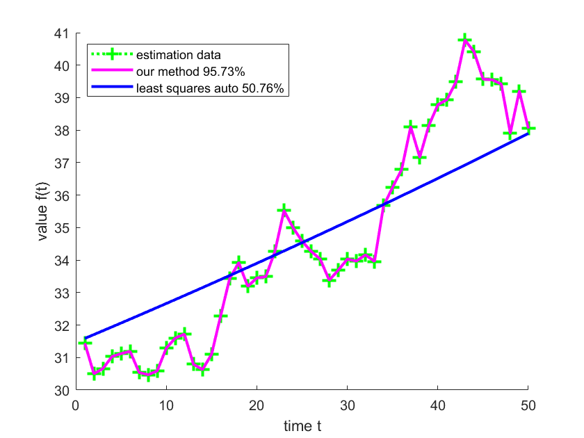
Obviously, our method could also be seen as a “prediction-error” method for improper learning of a linear dynamical system, i.e., forecasting its next output (measurement). As such, it can be applied to any time series. To exhibit this, we consider a real-world stock-market data first used in Liu et al. (2016) and attached in the supplementary material. (The data are believed to be related to the evolution of daily adjusted closing prices of stocks within the Dow Jones Industrial Average, starting on February 16, 1885. Unfortunately, the data are no longer available from the website of the authors of Liu et al. (2016).) We sample every four periods from the first 200 periods of the stock-market data and estimate the evolution for 50 periods. Our method is compared to a combination of least-squares algorithms implemented in Matlab™ System Identification Toolbox™ routine ssest with order set to $1$ (“least-squares auto”). The simulation results are shown in Figure 7. The percentages in the legend correspond to nrmse values (35), and both from the nrmse and the shape of the two curves, it seems clear that our method is superior.

Figure 7: The simulation results of our method and ”least-squares auto” system identification method implemented in Matlab™ System Identification Toolbox™, on stock market data used in Liu et al. (2016). The percentages in legend are corresponding nrmse values.

D.3 The Run-time

Additionally, we would like to present the run-time of our method as a function of the length of the time window, for univariate observations of the Experiment on Stock-market Data above. Figure 8 displays the run-time of our method with varying lengths $T$ of time windows from $5$ to $50$. We can see that the run-time of our method increases fast with the length $T$ of the time window, but that for modest $T$, the absolute run-time may be acceptable in many applications.

Figure 8: The run-time of our method as a function of $T$, which is the length of the time window. Notice that the solver is deterministic, so there is no variation of the run-time to report. While the run-time is exponential in $T$, it may be acceptable for modest $T$ in many applications.

References

- Åström (1965) Åström, K. J. Optimal control of markov processes with incomplete state information. Journal of Mathematical Analysis and Applications, 10(1):174 – 205, 1965. ISSN 0022-247X.
- Åström & Torsten (1965) Åström, K.-J. and Torsten, B. Numerical identification of linear dynamic systems from normal operating records. IFAC Proceedings Volumes, 2(2):96–111, 1965. ISSN 1474-6670. 2nd IFAC Symposium on the Theory of Self-Adaptive Control Systems, Teddington, UK, September 14-17, 1965.
- Akhiezer & Krein (1962) Akhiezer, N. I. and Krein, M. Some questions in the theory of moments, volume 2. American Mathematical Society, 1962.
- Anava et al. (2013) Anava, O., Hazan, E., Mannor, S., and Shamir, O. Online learning for time series prediction. In COLT 2013 - The 26th Annual Conference on Learning Theory, June 12-14, 2013, Princeton University, NJ, USA, 2013.
- Besserve et al. (2010) Besserve, M., Schölkopf, B., Logothetis, N. K., and Panzeri, S. Causal relationships between frequency bands of extracellular signals in visual cortex revealed by an information theoretic analysis. Journal of computational neuroscience, 29(3):547–566, 2010.
- Borwein & Wolkowicz (1981) Borwein, J. M. and Wolkowicz, H. Facial reduction for a cone-convex programming problem. Journal of the Australian Mathematical Society, 30(3):369–380, 1981.
- Boyd et al. (1994) Boyd, S., El Ghaoui, L., Feron, E., and Balakrishnan, V. Linear matrix inequalities in system and control theory, volume 15 of SIAM Studies in Applied Mathematics. SIAM, 1994.
- Burgdorf et al. (2016) Burgdorf, S., Klep, I., and Povh, J. Optimization of polynomials in non-commuting variables. Springer, 2016.
- Cafuta et al. (2011) Cafuta, K., Klep, I., and Povh, J. Ncsostools: a computer algebra system for symbolic and numerical computation with noncommutative polynomials. Optimization methods and Software, 26(3):363–380, 2011.
- d’Aspremont et al. (2005) d’Aspremont, A., Ghaoui, L. E., Jordan, M. I., and Lanckriet, G. R. A direct formulation for sparse pca using semidefinite programming. In Advances in neural information processing systems, pp. 41–48, 2005.
- Dixmier (1969) Dixmier, J. Les C*-algèbres et leurs représentations. Gauthier-Villars, Paris, France, 1969. English translation: C*-algebras (North-Holland, 1982).
- Faradonbeh et al. (2018) Faradonbeh, M. K. S., Tewari, A., and Michailidis, G. Finite time identification in unstable linear systems. Automatica, 96:342–353, 2018.
- Fukuda et al. (2001) Fukuda, M., Kojima, M., Murota, K., and Nakata, K. Exploiting sparsity in semidefinite programming via matrix completion i: General framework. SIAM Journal on Optimization, 11(3):647–674, 2001.
- Geiger et al. (2015) Geiger, P., Zhang, K., Schoelkopf, B., Gong, M., and Janzing, D. Causal inference by identification of vector autoregressive processes with hidden components. In International Conference on Machine Learning, pp. 1917–1925, 2015.
- Gelfand & Neumark (1943) Gelfand, I. and Neumark, M. On the imbedding of normed rings into the ring of operators in Hilbert space. Rec. Math. [Mat. Sbornik] N.S., 12(2):197–217, 1943.
- Harrison (1997) Harrison, P. J. Convergence and the constant dynamic linear model. Journal of Forecasting, 16(5):287–292, 1997.
- Hazan et al. (2017) Hazan, E., Singh, K., and Zhang, C. Learning linear dynamical systems via spectral filtering. In Advances in Neural Information Processing Systems, pp. 6702–6712, 2017.
- Hazan et al. (2018) Hazan, E., Lee, H., Singh, K., Zhang, C., and Zhang, Y. Spectral filtering for general linear dynamical systems. In Advances in Neural Information Processing Systems, pp. 4634–4643, 2018.
- Helton (2002) Helton, J. W. “Positive” noncommutative polynomials are sums of squares. Annals of Mathematics, 156(2):675–694, 2002.
- Henrion & Lasserre (2005) Henrion, D. and Lasserre, J.-B. Detecting global optimality and extracting solutions in gloptipoly. In Positive polynomials in control, pp. 293–310. Springer, 2005.
- Jansson (2003) Jansson, M. Subspace identification and arx modeling. In Proceedings of the 13th IFAC SYSID Symposium, pp. 1625–1630, 2003.
- Katayama (2006) Katayama, T. Subspace methods for system identification. Springer Science & Business Media, 2006.
- Klep et al. (2018) Klep, I., Povh, J., and Volcic, J. Minimizer extraction in polynomial optimization is robust. SIAM Journal on Optimization, 28(4):3177–3207, 2018.
- Kozdoba et al. (2019) Kozdoba, M., Marecek, J., Tchrakian, T., and Mannor, S. On-line learning of linear dynamical systems: Exponential forgetting in kalman filters. In The Thirty-Third AAAI Conference on Artificial Intelligence (AAAI-19), 2019. arXiv preprint arXiv:1809.05870.
- Kungurtsev & Marecek (2018) Kungurtsev, V. and Marecek, J. A two-step pre-processing for semidefinite programming. arXiv preprint arXiv:1806.10868, 2018.
- Leslie (1945) Leslie, P. H. On the use of matrices in certain population mathematics. Biometrika, 33(3):183–212, 11 1945. ISSN 0006-3444.
- Liu et al. (2016) Liu, C., Hoi, S. C. H., Zhao, P., and Sun, J. Online arima algorithms for time series prediction. AAAI’16, 2016.
- Liu & Vandenberghe (2009) Liu, Z. and Vandenberghe, L. Semidefinite programming methods for system realization and identification. In Proceedings of the 48h IEEE Conference on Decision and Control (CDC) held jointly with 2009 28th Chinese Control Conference, pp. 4676–4681, Dec 2009. doi: 10.1109/CDC.2009.5400177.
- Ljung (1998) Ljung, L. System Identification: Theory for the User. Pearson Education, 1998.
- Löfberg (2009) Löfberg, J. Pre- and post-processing sum-of-squares programs in practice. IEEE Transactions on Automatic Control, 54(5):1007–1011, 2009.
- Majumdar et al. (2019) Majumdar, A., Hall, G., and Ahmadi, A. A. Recent scalability improvements for semidefinite programming with applications in machine learning, control, and robotics. Annual Review of Control, Robotics, and Autonomous Systems, 3, 2019.
- McCullough (2001) McCullough, S. Factorization of operator-valued polynomials in several non-commuting variables. Linear Algebra and its Applications, 326(1-3):193–203, 2001.
- Mevissen & Kojima (2010) Mevissen, M. and Kojima, M. Sdp relaxations for quadratic optimization problems derived from polynomial optimization problems. Asia-Pacific Journal of Operational Research, 27(01):15–38, 2010.
- Pearl (2009) Pearl, J. Causality. Cambridge university press, 2009.
- Permenter & Parrilo (2018) Permenter, F. and Parrilo, P. Partial facial reduction: simplified, equivalent sdps via approximations of the psd cone. Mathematical Programming, 171(1-2):1–54, 2018.
- Pironio et al. (2010) Pironio, S., Navascués, M., and Acín, A. Convergent relaxations of polynomial optimization problems with noncommuting variables. SIAM Journal on Optimization, 20(5):2157–2180, 2010.
- Recht et al. (2010) Recht, B., Fazel, M., and Parrilo, P. A. Guaranteed minimum-rank solutions of linear matrix equations via nuclear norm minimization. SIAM review, 52(3):471–501, 2010.
- Rosenfeld et al. (2020) Rosenfeld, A., Cohen, M., Kraus, S., and Keshet, J. Online prediction of time series with assumed behavior. Engineering Applications of Artificial Intelligence, 88:103358, 2020. ISSN 0952-1976.
- Sarkar & Rakhlin (2019) Sarkar, T. and Rakhlin, A. Near optimal finite time identification of arbitrary linear dynamical systems. In Chaudhuri, K. and Salakhutdinov, R. (eds.), Proceedings of the 36th International Conference on Machine Learning, volume 97 of Proceedings of Machine Learning Research, pp. 5610–5618, Long Beach, California, USA, 09–15 Jun 2019. PMLR.
- Sarkar et al. (2019) Sarkar, T., Rakhlin, A., and Dahleh, M. A. Finite-time system identification for partially observed lti systems of unknown order. arXiv:1902.01848 [cs.SY], 2019. doi: https://arxiv.org/abs/1902.01848.
- Segal (1947) Segal, I. E. Irreducible representations of operator algebras. Bulletin of the American Mathematical Society, 53(2):73–88, 1947.
- Shapiro (2019) Shapiro, A. Statistical inference of semidefinite programming. Mathematical Programming, 174(1-2):77–97, 2019.
- Simchowitz et al. (2018) Simchowitz, M., Mania, H., Tu, S., Jordan, M. I., and Recht, B. Learning without mixing: Towards a sharp analysis of linear system identification. In Conference On Learning Theory, pp. 439–473, 2018.
- Simchowitz et al. (2019) Simchowitz, M., Boczar, R., and Recht, B. Learning linear dynamical systems with semi-parametric least squares. arXiv preprint arXiv:1902.00768, 2019.
- Tangirala (2014) Tangirala, A. K. Principles of system identification: theory and practice. Crc Press, 2014.
- Tsiamis & Pappas (2020) Tsiamis, A. and Pappas, G. Online learning of the kalman filter with logarithmic regret. arXiv preprint arXiv:2002.05141, 2020.
- Tsiamis & Pappas (2019) Tsiamis, A. and Pappas, G. J. Finite sample analysis of stochastic system identification. arXiv preprint arXiv:1903.09122, 2019.
- Tsiamis et al. (2019) Tsiamis, A., Matni, N., and Pappas, G. J. Sample complexity of Kalman filtering for unknown systems. arXiv preprint arXiv:1912.12309, 2019.
- Tunçel (2000) Tunçel, L. Potential reduction and primal-dual methods. In Handbook of semidefinite programming, pp. 235–265. Springer, 2000.
- Van Overschee & De Moor (1996) Van Overschee, P. and De Moor, B. Subspace identification for linear systems. Theory, implementation, applications. Incl. 1 disk, volume xiv. 01 1996. ISBN 0-7923-9717-7. doi: 10.1007/978-1-4613-0465-4.
- Vazirani (2013) Vazirani, V. V. Approximation algorithms. Springer Science & Business Media, 2013.
- West & Harrison (1997) West, M. and Harrison, J. Bayesian Forecasting and Dynamic Models (2nd ed.). Springer-Verlag, Berlin, Heidelberg, 1997. ISBN 0-387-94725-6.
- Wittek (2015) Wittek, P. Algorithm 950: Ncpol2sdpa—sparse semidefinite programming relaxations for polynomial optimization problems of noncommuting variables. ACM Transactions on Mathematical Software (TOMS), 41(3):1–12, 2015.
- Yamashita et al. (2003) Yamashita, M., Fujisawa, K., and Kojima, M. Implementation and evaluation of sdpa 6.0 (semidefinite programming algorithm 6.0). Optimization Methods and Software, 18(4):491–505, 2003.