Bell’s Theorem:
A parametric and geometric perspective

A parameterized operational representation of an EPRB experiment is presented that facilitates direct comparisons among mathematical models that characterize the concepts of local hidden variables, the factorization condition, remote context independence, remote outcome independence, local causality, and predictability. The different models and conditions are derived from a common template, differentiated by parameter adjustment only. Supplementing this simple, direct comparison are figures and tables that illustrate the proofs and examples. This perspective enables new and easier proofs of some existing results.

All models are wrong but some are useful. George Box

1 Introduction

Several decades after John Bell’s famous paper [2], considerable debate remains over the meaning and import of Bell’s Theorem, especially since Bell himself put forward variations in [4], [5], and [9] as his ideas evolved. Consider the Google Scholar citations [13]) in Fig. 1 that show the rising number of papers per year that cite John Bell, 1982-2019.

Figure 1: Citations of Bell’s papers by year: 1982-2019 (Google Scholar)

Many debates center around what it is that Bell actually proved, for example, what combination of determinism, reality, or locality enables the derivation of Bell’s inequality. For some excellent discussions of this issue (and more) see [14], [15], [28], [32], and [33] in the book the book “Quantum Nonlocality and Reality: 50 Years of Bell’s Theorem” edited by Mary Bell and Shan Gao ([12]. This volume contains 26 papers by different authors. These papers all rightfully recognize John Bell’s major contributions to the foundations of quantum theory, but there still remains disagreement about some of the details of his work. T. Maudlin’s paper [25] and the related online lecture [26] offer thought-provoking opinions about misunderstandings not only by the general public but also by some in the mainstream physics community.

One difficulty is that many of the terms mean different things to different people (common to all of human discourse, of course!). “Locality” seems to be the most difficult to pin down, being attached in one way or another to (at least) four mathematical definitions, not to mention the confusion brought on by the everyday use of the term.

One paper and one article that particularly influenced the approach in this paper are those of of H. Wiseman [36] and A. Shimony [31], respectively. Wiseman follows the evolution of Bell’s thinking as represented by Bell’s 1964 and 1976 papers ( [2] and [4]), and along the way creates a complete anthology of the main concepts, with precise definitions. Similarly, Shimony’s excellent discussion of the many concepts of locality (among other things) is accompanied by clear mathematical definitions.

The main contribution of this paper is a mathematical framework that unifies many of the concepts traditionally discussed in the context of Bell’s Theorem into a single parameterized modeling template. These concepts include local hidden variables, factorization, predictability, locally causality, remote context independence, and remote outcome independence. The advantages of this approach are:

• Each concept is represented by a simple change to the symbolic form or numeric values of the parameters.

• Striking visualizations that demonstrate, much more than a simple inequality, just how difficult it is to replicate all of the characteristics of QM with models based on the concepts of reality, locality, and/or predictability.

• Proofs of existing results, such as the CHSH inequalities or Fine’s Theorem, become trivial or at least short and visually intuitive .

Figure 2: Relationships among the model types and conditions. All terms will be defined and relationships proved in the body of the paper.

The body of the paper is to dedicated to defining the terms and justifying all of the relationships illustrated in Fig. 2. This diagram also appears in Sec. 3 after the relevant terms are defined. It is duplicated here to give the reader an idea of the purpose and scope of the paper.

1.1 Assumptions and scope

The philosophical viewpoint in this paper is to clearly separate a model type or instance from its interpretation and/or significance. A rationale is given for its name based on historical context, but no judgment is made whether this is justified. The main purpose of this paper is simply to organize and classify many of the modeling types related to Bell’s Theorem so as to form a basis for a follow-on discussion of whether or not these purely mathematical constructions have true relevance to the physics involved. This is not a unique endeavor, but perhaps this collection of many models “under one roof” may aid intuition and understanding.

The analysis and results in this paper are derived from a parameterized joint probability mass function (pmf) on the operational variables in the EPRB experiment. The four operational variables comprise Alice’s outcome and measurement detector setting and Bob’s outcome and measurement detector setting. A model type is distinguished by its particular pmf parameterization. These model types include quantum mechanics, (QM), “Bell real” (local hidden variables), “Bell local” (satisfies the factorization condition), “predictable” (certain conditional probabilities can only be 0 or 1), and for completeness, two special model types called “generic” and “trivial”. In addition other properties related to locality (local causality, context independence, outcome independence) can be discussed in terms of these parameterizations.

All results are based on this paradigm. It might seem quite arbitrary to call a given model a “local, hidden variables” model just because of some specific assignment of parameters to its generic pmf. This where the hidden variables come into play. When the operational variables are combined with the hidden variables, various concepts of reality and/or locality can be introduced by the nature of the joint probability density on the hidden variables. In short, the approach in this paper differs from the traditional approach in that the only role of the hidden variables is to give a rationale for the name of the resulting model, not to be part of the modeling analysis. This process is explained in detail, with specific examples, in Sec.’s 2.1 and 2.2.

Certain aspects of this approach may be criticized as being “non-contextual”. For a discussion of contexuality, see for example A. Shimony’s paper [30]. In that paper, Shimony references the papers of Gleason [20] and Bell [3] that started the discussion of the distinction between non-contextual and contextual theories.

There are authors who repudiate the non-contextual approach altogether, in particualr Hess, De Raedt, and Michielsen in [22], noting that because it implicitly assumes “counterfactual definiteness”, it is irrelevant to any EPRB-like experiment and also to Einstein’s original concerns. See also the Wikipedia article [35] which discusses Hess’s claims, among others.

However, it is claimed that, in this paper, since the non-contextual assumptions are specifically confined to the hidden variable portion of the combined joint probability distribution, the results derived from the operational variable portion only are not necessarily nullified. In fact this approach isolates the potentially non-contextual aspects by clearly separating the roles of the operational and hidden variables. One can disagree with the connection of the model name to a particular model type, essentially agreeing with [22], or one can forget the hidden variable part, and draw conclusions based solely on the resulting operational-variable models.

1.2 Mathematica

The computational workhorse behind everything in this paper is the Wolfram language platform Mathematica, including the initial idea exploration and feasibility analysis, the heavy-duty matrix generation and calculations, function optimization and equation solving, the computation of expectations, marginal and conditional distributions, and especially the generation of the plots and visualizations. Future plans include uploading some of the more interesting routines and visualizations to the Wolfram Demonstrations Project website.

2 Definitions, notation, and terminology

Definition 1.

The operational random variables (r.v.’s) consist of Alice and Bob’s outcomes and detector settings:
$A$ = a random variable representing Alice’s outcome,
$D_{A}$ = a random variable representing Alice’s detector setting,
$B$ = a random variable representing Bob’s outcome,
$D_{B}$ = a random variable representing Bob’s detector setting.
The operational r.v.’s correspond to something in the experiment that is either observed (e.g., outcomes) or manipulated (e.g., detector settings).

It is standard in the literature to let $a$ and $a^{\prime}$ stand for Alice’s two measurement angle choices and $b$ and $b^{\prime}$ stand for Bob’s two measurement angle choices. Based on this, define the detector setting random variables and associated probabilities as follows.

Definition 2.

Meaning of detector setting values:
$D_{A}=-1$ means “Alice chooses detector angle $a$”,
$D_{A}=+1$ means “Alice chooses detector angle $a^{\prime}$”,
$D_{B}=-1$ means “Bob chooses detector angle $b$”,
$D_{B}=+1$ means “Bob chooses detector angle $b^{\prime}$”.

Definition 3.

Detector setting probabilities
$\delta_{ab}=P\left(D_{A}=-1,D_{B}=-1\right)$,
$\delta_{ab^{\prime}}=P\left(D_{A}=-1,D_{B}=+1\right)$,
$\delta_{a^{\prime}b}=P\left(D_{A}=+1,D_{B}=-1\right)$,
$\delta_{a^{\prime}b^{\prime}}=P\left(D_{A}=+1,D_{B}=+1\right)$,
$\delta_{a}=\delta_{ab}+\delta_{ab^{\prime}}\text{ and }\delta_{a^{\prime}}=\delta_{a^{\prime}b}+\delta_{a^{\prime}b^{\prime}},$
$\delta_{b}=\delta_{ab}+\delta_{a^{\prime}b}\text{ and }\delta_{b^{\prime}}=\delta_{ab^{\prime}}+\delta_{a^{\prime}b^{\prime}}.$

Definition 4.

A pmf (probability mass function) is a finite ordered set of real numbers $\left(q_{1},q_{2},\text{...},q_{n}\right)$ such that $q_{k}\geq 0$ all $k$ and $\sum_{k=1}^{n}q_{k}=1$.

Definition 5.

As shown in Table 1, a model type (or simply model) is defined by specifying the symbolic form of the parameters $\boldsymbol{\gamma}=(\gamma_{1},\gamma_{2},...,\gamma_{16})$ , while a model instance is defined by specifying numerical values for these same 16 parameters.

Table 1: The generic probability model: operational r.v.’s and associated generic pmf.

Note the constraints in the last row of Table 1 make the last column a pmf.

2.1 Hidden variables

In an EPRB-like experimental context (Einstein-Podolsky-Rosen-Bohm, see Sec. 3.1 in [19]), one can imagine, in addition to the main random variables $(A,B,D_{A},D_{B})$ of operational interest, an additional set of hidden variables:

Definition 6.

The hidden random variables (r.v.’s), denoted collectively by $\Lambda$, represent unseen information in an EPRB-like experiment. In other words, these variables cannot be directly observed or manipulated. They are sometimes called supplementary varaiables–see Aspect [1].

These hidden variables $\Lambda$ can be a single random variable or a random vector, the components of which may be discrete and/or continuous r.v.’s. For the models discussed in this paper, it will be assumed that given a pmf on the hidden r.v.’s $\Lambda$, then there exists a joint pmf on $(A,B,D_{A},D_{B},\Lambda)$ where the marginal hidden r.v.’s pmf matches the original. In particular, this means that, after computing the marginal pmf on the operational r.v.’s, further mention of the hidden r.v.’s can be suppressed. The most general form of such a (marginalized) model based on the operational r.v.’s only is shown in Table 1 (hence the name “generic”). Put another way, the hidden r.v.’s are introduced to mathematically characterize certain concepts, like “reality” or “locality”, but once the marginal pmf on $(A,B,D_{A},D_{B})$ is computed based on the full joint pmf on $(A,B,D_{A},D_{B},\Lambda)$, all subsequent results are based solely on the marginal pmf, as shown in Table 1.

2.2 The Bell real and Bell local model types

As a specific example, assume that $\Lambda=(A_{1},A_{2},B_{1},$ $B_{2})$, taking values in $\{-1,1\}^{4}$, with two different potential pmf’s assumed, as shown in Table 2.

Table 2: Hidden variable Bell real and Bell local model pmfs.

The rationale for the pmf names will be explained in Sec.’s 2.2.1 and 2.2.3. The full joint pmf’s for the 64 possible outcomes of both operational and hidden r.v.’s $(A,B,D_{A},D_{B},A_{1},A_{2},B_{1},B_{2})$ are shown in Tables 3 and 4, split over two pages.

Table 3: The combined model (first half).

Table 4: The combined model (second half).

To see how this full joint pmf is connected to the corresponding (hidden r.v.) marginal pmf’s in Table 2, consider row 50 in Table 4, shown in red for easy identification. The four numbers $(A_{1},A_{2},B_{1},B_{2})=(1,1,-1,-1)$ in row 50 represent the prepared definite outcomes, awaiting only Alice’s and Bob’s measurement setting choices.

Also note that $D_{A}=-1,D_{B}=+1$, which means that Alice uses her first measurement setting and Bob uses his second. Therefore, Alice gets the measurement outcome $A=A_{1}=1$ and Bob gets the measurement outcome $B=B_{2}=-1$. Hence their joint measurement outcome is $(A,B)=(1,-1)$, so finally the operational r.v.’s are $\left(A,B,D_{A},D_{B}\right)=(1,-1,-1,1)$ and the full row 50 is $(A,B,D_{A},D_{B},A_{1},A_{2},B_{1},B_{2})=(1,-1,-1,1,1,1,-1,-1)$.

The probabilities in the “Bell real” and “Bell local” columns of row number 50, namely $\rho_{13}\delta_{ab^{\prime}}$ and $\alpha_{3}\alpha_{4}\beta_{1}\beta_{2}\delta_{ab^{\prime}}$, resepectively, come from the fact that $\left(A_{1},A_{2},B_{1},B_{2}\right)=(1,1,-1,-1)$ is in the 13th row of Table 2, hence has probability $\rho_{13}$ in column 5 and $\alpha_{3}\alpha_{4}\beta_{1}\beta_{2}$ in column 6. When combined with the probability of Alice choosing her first measurement setting and Bob choosing his second measurement setting, which is $\delta_{ab^{\prime}}$, this yields overall probabilities of $\rho_{13}\delta_{ab^{\prime}}$ and $\alpha_{3}\alpha_{4}\beta_{1}\beta_{2}\delta_{ab^{\prime}}$ in row 50 of the last two columns of Table 4, respectively. Similarly for the other 63 rows (exercise for the reader to check!).

The resulting marginal pmf’s of the operational r.v.’s for both the Bell real and Bell local models are shown in Table 5.

Table 5: Operational r.v. Bell real and Bell local model pmfs.

The constraints in the last row of Table 5 guarantee that entries in both the “Bell real” and “Bell local” columns form a pmf.

2.2.1 Rationale for the name Bell real

Note that $\Lambda=(A_{1},A_{2},B_{1},B_{2})$ denotes four discrete hidden r.v.’s taking values in $\{-1,+1\}$ as shown in Table 2, along with the symbolic pmf shown in the “Bell real” (5th) column. These four numbers $(A_{1},A_{2},B_{1},B_{2})$ represent prepared definite, i.e. real, outcomes, awaiting only Alice’s and Bob’s measurement setting choices. That is, the photon sent to Alice is “encoded” with the definite outcomes $(A_{1},A_{2})$ and similarly the one sent to Bob is “encoded” with definite outcomes $(B_{1},B_{2})$. For example when Alice uses her first measurement setting ($D_{A}=-1$, i.e., angle $a$), she observes the outcome $A=A_{1}$, and when she uses her second measurement setting ($D_{A}=+1$, i.e., angle $a^{\prime}$), she observes the outcome $A=A_{2}$. Similarly for Bob.

This explains the “real” part of the name. It turns out that all instances of the “Bell real” model type also satisfy the remote context independence (RCI) condition, which is a (weak) form of locality (see Sec. 2.2.2 and Thm. 11 in Sec. 10.2). This characterization is similar to the description of a “local hidden variables theory” in the textbook by Schumacher and Westmoreland [29], which in turn has been chacterized as a fair representation of Bell’s original intentions by Wiseman [36].

2.2.2 Definitions of terms related to locality

An excellent discussion of concepts related to locality can be found in Abner Shimony’s article [31]. The fundamental concepts in the article are remote context independence (often called parameter independence), remote outcome independence (often called outcome independence), and the factorization condition. The following definitions translate these concepts into the formalism of this paper. Note that these definitions involve the operational r.v.’s only.

Definition 7.

Remote Context Independence (RCI):

$$P(A=s|D_{A}=t,D_{B}=u)=P(A=s|D_{A}=u)$$

and

$$P(B=t|D_{A}=u,D_{B}=v)=P(B=t|D_{B}=v)$$

for all $(s,t,u,v)\in\{-1,1\}^{4}$.

Definition 8.

Remote Outcome Independence (ROI):

$$P(A=s|B=t,D_{A}=u,D_{B}=v)=P(A=t|D_{A}=u,D_{B}=v)$$

and

$$P(B=t|A=s,D_{A}=u,D_{B}=v)=P(B=t|D_{A}=u,D_{B}=v)$$

for all $(s,t,u,v)\in\{-1,1\}^{4}$. That is, the outcomes $A$ and $B$ are conditionally independent given the detector-setting pair $(D_{A},D_{B})$.

Definition 9.

Factorization condition (FC):

$$P(A=s,B=t|D_{A}=u,D_{B}=v)=P(A=s|D_{A}=u)\times P(B=t|D_{B}=v)$$

for all $(s,t,u,v)\in\{-1,1\}^{4}$.

Both Shimony [31] and Wiseman [36] use the term “Bell local” to describe models that satisfy the factorization condition.

Definition 10.

(Bell locality): A model instance will be called Bell local iff its associated operational r.v.’s $\left(A,B,D_{A},D_{B}\right)$ satisfy the factorization condition.

The definition of local causality is based on [36], which Wiseman uses to characterize Bell’s ideas about local causality in [4]. This is intended to capture the idea that anything outside of Alice’s past light cone, such as Bob’s settings or outcomes, are statistically irrelevant to her outcome, and similarly for Bob’s outcome with regard to Alice’s actions or observations.

Definition 11.

(Local causality or LC) A model instance is said to be locally causal, or to satisfy local causality, if

$$P(A=s|B=t,D_{A}=u,D_{B}=v)=P(A=s|D_{A}=u)$$

and

$$P(B=t|A=s,D_{A}=u,D_{B}=v)=P(B=t|D_{B}=v)$$

for all $(s,t,u,v)\in\{-1,1\}^{4}$.

2.2.3 Rationale for the name Bell local

The following construction, based on the hidden variables, results in a marginal pmf on the operational r.v.’s that satisfies the factorization condition, hence making it a “Bell local” model. Though the notation is different, it is equivalent to Fine’s discussion of a stochastic hidden variables model being factorizable in [18]. Assume the hidden r.v.’s $(A_{1},A_{2},B_{1},B_{2})$ are independent and define

$$\alpha_{1}=P(A_{1}=-1),\;\beta_{1}=P(B_{1}=-1),$$

$$\alpha_{3}=P(A_{1}=+1),\;\beta_{3}=P(B_{1}=+1),$$ (1)

$$\alpha_{2}=P(A_{2}=-1),\;\beta_{2}=P(B_{2}=-1),$$

$$\alpha_{4}=P(A_{2}=+1),\;\beta_{4}=P(B_{2}=+1).$$

Claim that these assumptions result in the pmf for a (hidden variable) Bell local model as shown in Table 2. For example,

$$P(\left(A_{1},A_{2},B_{1},B_{2}\right)=(1,1,-1,-1))=\alpha_{3}\alpha_{4}\beta_{1}\beta_{2}.$$

Note that this matches the last entry in row 13 of Table 2. Similarly for any of the other 15 possible outcomes $(A_{1},A_{2},B_{1},B_{2})$. Also, from Eq. 1, it is easy to see that the following constraints must hold for the parameters of any Bell local model instance.

$$\alpha_{1}+\alpha_{3}=\alpha_{2}+\alpha_{4}=1,\;\beta_{1}+\beta_{3}=\beta_{2}+\beta_{4}=1.$$ (2)

2.2.4 Summary of the meaning of the terms Bell real and Bell local

1. “Bell real” conforms to the usual notion of a “local hidden variables” or “local realism” theory in the spirit of Bell [2], Aspect [1], Shumacher and Westmoreland [29], and Clauser, Horne, Shimony, and Holt [17]. Here “local” refers to remote context independence (RCI) of Def. 7, which is a weaker condition than the factorization condition (FC) of Def 9. Thus in order to avoid confusion over two different uses of the term “local” in this paper, locality is not mentioned explicitly in the term “Bell real”. Keep in mind, however, that a Bell real model instance is still “local” in the sense that it satisfies RCI (Thm. 11 in Sec. 10).

2. “Bell local” is defined as being equivalent to satisfaction of the factorization condition (Def. 9 and 10), based on Shimony [31] and Wiseman [36].

2.3 The 5 main model types

Table 6 shows the symbolic form of the parameters $\boldsymbol{\gamma}$ for the five main model types of interest in this paper, based on the operational r.v.’s. The parameter constraints are shown in the bottom row of the table for each model type.

If the joint detector-setting probabilities satisfy $0<\delta_{ab},\delta_{ab^{\prime}},\delta_{a^{\prime}b},\delta_{a^{\prime}b^{\prime}}<1$ strictly, then the parameters $\boldsymbol{\gamma}=(\gamma_{1},\gamma_{2},...,\gamma_{16})$ can be identified with the conditional probabilities $P(A,B|D_{A},D_{B})$, e.g.,

$$P(A=-1,B=-1|D_{A}=-1,D_{B}=-1)=\frac{\gamma_{1}\delta_{ab}}{(\gamma_{1}+\gamma_{5}+\gamma_{9}+\gamma_{13})\delta_{ab}}=\gamma_{1},$$

since $\gamma_{1}+\gamma_{5}+\gamma_{9}+\gamma_{13}=1$; see Table 1 in Def. 5. In this example, if $\delta_{ab}=0$, then the conditional probability on the LHS is undefined, whereas $\gamma_{1}$ presumably is defined. For this reason, it will be assumed that the detector-setting probabilities are all strictly between 0 and 1 unless explicitly stated otherwise. Note that the full pmf’s for each model type can be recovered by multiplying each entry in the appropriate column by the appropriate detector-setting probability from $\{\delta_{ab},\delta_{ab^{\prime}},\delta_{a^{\prime}b},\delta_{a^{\prime}b^{\prime}}\}$. For example, the resulting pmf’s for the Bell real and Bell local model types are shown in Table 5.

Table 6: The five main modeling types are defined by the symbolic form of their conditional probabilities $P(A,B|D_{A},D_{B})$.

2.4 Correlations, consistency and the CHSH inequalities

Definition 12.

For any row or column vector $\boldsymbol{p}$, $a\leq\boldsymbol{p}\leq b$ means that every entry $p_{k}$ of $\boldsymbol{p}$ satisfies $a\leq p_{k}\leq b$.

Definition 13.

If $-1\leq\boldsymbol{p}=(w,x,y,z)\leq 1$ then $\boldsymbol{p}$ will be called a correlation vector.

Definition 14.

The correlation vector $\boldsymbol{c}$ associated with the generic probability model of Table 1 is defined by the conditional expectations

$$\boldsymbol{c}^{T}=\left(\begin{array}[]{l}E[AB|D_{A}=-1,D_{B}=-1]\\ E[AB|D_{A}=-1,D_{B}=1]\\ E[AB|D_{A}=1,D_{B}=-1]\\ E[AB|D_{A}=1,D_{B}=1]\\ \end{array}\right)=\left(\begin{array}[]{l}\gamma_{1}-\gamma_{5}-\gamma_{9}+\gamma_{13}\\ \gamma_{2}-\gamma_{6}-\gamma_{10}+\gamma_{14}\\ \gamma_{3}-\gamma_{7}-\gamma_{11}+\gamma_{15}\\ \gamma_{4}-\gamma_{8}-\gamma_{12}+\gamma_{16}\\ \end{array}\right).$$ (3)

Note 1.

Compare this way of expressing a model instance correlations as opposed to the traditional way involving the hidden variables.

$$\left\langle A_{1}B_{1}\right\rangle =E\left[AB\left|D_{A}\right.=-1,D_{B}=-1\right],$$

$$\left\langle A_{1}B_{2}\right\rangle =E\left[AB\left|D_{A}\right.=-1,D_{B}=1\right],$$ (4)

$$\left\langle A_{2}B_{1}\right\rangle =E\left[AB\left|D_{A}\right.=1,D_{B}=-1\right],$$

$$\left\langle A_{2}B_{2}\right\rangle =E\left[AB\left|D_{A}\right.=1,D_{B}=1\right].$$

Notice that the modeling paradigm in this paper emphasizes the conditional nature of the correlations (expectations on the right), unlike the traditional presentation (on the left, involving the hidden r.v.’s $\left(A_{1},A_{2},B_{1},B_{2}\right)$), where it appears that the expectations are all computed with respect to the same expectation operator.

Definition 15.

Consistency and achievability: Let $\boldsymbol{p}=(w,x,y,z)$ be an arbitrary correlation vector. Then $\boldsymbol{p}$ is said to be consistent with a model instance with parameters $\boldsymbol{\gamma}=(\gamma_{1},\gamma_{2},...,\gamma_{16})$ if $\boldsymbol{p}=\boldsymbol{c}$ from Def. 14. Another way of saying this is that $\boldsymbol{p}=(w,x,y,z)$ is an achievable set of correlations by the model type in question.

Note 2.

This is a very specific flavor of consistency, which was worked out in a much more general setting long ago by Vorobev [34]. This reference came to the author’s attention via Hess and Philipp [23].

Definition 16.

The s-functions are the 4 components of the linear map $\boldsymbol{s}=\left(s_{1},s_{2},s_{3},s_{4}\right):R^{4}\to R^{4}$ represented by the matrix

$$S=\left(\begin{array}[]{cccc}-1&1&1&1\\ 1&-1&1&1\\ 1&1&-1&1\\ 1&1&1&-1\\ \end{array}\right).$$

For example, $s_{2}(w,x,y,z)=w-x+y+z$ and similarly for the other three.

Definition 17.

If $\boldsymbol{p}=(w,x,y,z)$ is a correlation vector, then it satisfies the CHSH inequalities if $-2\leq S\boldsymbol{p}^{T}\leq 2$. There are 8 CHSH inequalities (4 pairs).

Note 3.

The CHSH inequalities represent a generaliztion of Bell’s original inequality [2], as formulated in Clauser, Horne, Shimony, and Holt [17] and also in Bell [7]. See also Shimony [31], Aspect [1], and Schumacher and Westmoreland [29].

Note 4.

In this paper, whenever a phrase such as “model instance X satisfies the CHSH inequalities” is used, it means that the correlations of model instance X satisfy the CHSH inequalities.

The following matrix makes it easy to compute the correlations of any model instance, and in combination with the $S$ matrix, to compute its $s$-functions.

Definition 18.

The correlation matrix $C=$

$$\left(\begin{array}[]{cccccccccccccccc}1&0&0&0&-1&0&0&0&-1&0&0&0&1&0&0&0\\ 0&1&0&0&0&-1&0&0&0&-1&0&0&0&1&0&0\\ 0&0&1&0&0&0&-1&0&0&0&-1&0&0&0&1&0\\ 0&0&0&1&0&0&0&-1&0&0&0&-1&0&0&0&1\end{array}\right).$$

The correlation matrix turns a set of generic model parameters

$$\boldsymbol{\gamma}=(\gamma_{1},\gamma_{2},...,\gamma_{16})$$

into the associated set of correlations

$$\boldsymbol{c}^{T}=C\boldsymbol{\gamma}^{T}=\left(\begin{array}[]{cccc}\gamma_{1}-\gamma_{5}-\gamma_{9}+\gamma_{13}\\ \gamma_{2}-\gamma_{6}-\gamma_{10}+\gamma_{14}\\ \gamma_{3}-\gamma_{7}-\gamma_{11}+\gamma_{15}\\ \gamma_{4}-\gamma_{8}-\gamma_{12}+\gamma_{16}\end{array}\right)$$ (5)

and the $s$-function values are given by

$$\boldsymbol{s}^{T}=(s_{1},s_{2},s_{3},s_{4})^{T}=S\boldsymbol{c}^{T}=SC\boldsymbol{\gamma}^{T}.$$ (6)

2.5 Predictability

The idea behind “predictability” is that Alice’s and Bob’s outcomes, conditioned on a given pair of detector settings, should be a sure bet – for or against. This is achieved by making a specified set of conditional probabilities all either 0 or 1. As a result, all of the correlations are $\pm 1$, meaning that Alice’s and Bob’s outcomes are either perfectly correlated or perfectly anti-correlated, which seems appropriate for a model named “predictable”. See Sec. 5.6. It turns out that “perfectly correlated” model instances already have interesting properties, so this section starts out with a brief discussion of them.

Definition 19.

A generic (maximal) model instance will be called perfectly correlated (PC) if it’s correlations are all $\pm 1$. In other words,

$$w=\gamma_{1}-\gamma_{5}-\gamma_{9}+\gamma_{13}=\pm 1,\;x=\gamma_{2}-\gamma_{6}-\gamma_{10}+\gamma_{14}=\pm 1,$$

$$y=\gamma_{3}-\gamma_{7}-\gamma_{11}+\gamma_{15}=\pm 1,\;z=\gamma_{4}-\gamma_{8}-\gamma_{12}+\gamma_{16}=\pm 1.$$ (7)

Since the subsets of $\gamma_{k}$’s that go into defining each of the correlations are mutually disjoint, it is clear that $(w,x,y,z)$ can be any of 16 possible sequences of $\pm 1$’s. The $s$-functions are determined by the patterns of the $\pm 1$’s according to Table 7.

Table 7: All possible values of $s$-functions for a perfectly correlated model instance.

Although the arrangement of numbers in any row of the last four columns might be different, the numbers that appear will be the same. The following theorem is then evident by inspection.

Theorem 1.

If a generic model instance is perfectly correlated, then either all of its $s$-functions satisfy all of the CHSH inequalities or exactly one of its $s$-functions violates one of the Tsirelson bounds ($\pm 2\sqrt{2}$ – see Sec. 5.2.2).

In summary, a generic model instance with perfect correlations is inconsistent with at least some of the behaviors of QM. Now on to predictability itself, a stronger notion than perfect correlation.

Definition 20.

A generic model instance is called predictable if all of the conditional probabilities

$$P(A=s,B=t|D_{A}=u,D_{B}=v)=0\text{ or }1\text{ for all }(s,t,u,v)\in\{-1,1\}^{4}.$$

When combined with the basic generic model constraints (Def. 5 or Table 6), it must be the case that all $\gamma_{k}=0$ except that exactly four of them are equal to 1, say $\gamma_{j_{1}},\gamma_{j_{2}},\gamma_{j_{3}},\gamma_{j_{4}}$, where

$$j_{1}\in\{1,5,9,13\},j_{2}\in\{2,6,10,14\},j_{3}\in\{3,7,11,15\},\text{ and }j_{4}\in\{4,8,12,16\}.$$

Note 5.

The term “predictable” is based on Cavalcanti’s and Wiseman’s discussion of the difference between determinism and predictability in [16]. Their distinction is based on the difference between a pmf in a model and the corresponding observed frequencies in an actual experiment. Note however, in the paper you are reading now, “predictable” is being applied to describe a pmf in a model. The reason is that terms like “determine”, “determinism”, or “deterministic” are traditionally used to describe Bell’s original approach [2] of postulating “response functions” such as $A(a,\lambda)$, which represents a determinate outcome for Alice of $\pm 1$ as a function of her detector angle setting $a$ and the system state as represented by the “hidden variable” $\lambda$ (see for example, Aspect [1], CHSH [17], Fine [18], or Wiseman [36]). The resulting “local, hidden variables” model does not necessarily have all correlations equal to $\pm 1$. In fact it leads to the “Bell real” model type of this paper (see Sec. 2.2), instances of which can have any correlations, as long as they satisfy the CHSH inequalities. This includes the predictable type 1 model instances (see Def. 21), but it also includes many non-predictable model instances as well, in the sense of this paper. Hence it is better to use a term like “predictable” rather than produce even more confusion from overloading the word “deterministic”.

Theorem 2.

Every predictable model instance is also perfectly correlated.

Proof.

Consider Eqn. 7 (Def. 19) and the definition of (generic) predictability (Def. 20). Since exactly one $\gamma_{k}$ in each correlation $w,x,y,\text{ or }z$ is $1$, and all the others $0$, they are all obviously $\pm 1$. ∎

2.5.1 Predictable model types

Based on Def. 20, a predictable model instance is determined by choosing one $\gamma_{k}$ from a possible four out of each of four mutually disjoint collections of $\gamma_{k}$’s. Hence there are exactly $4^{4}=256$ different predictable model instances. This collection of instances can be neatly broken down into categories based on, first of all, whether or not they satisfy all 8 CHSH inequalities, and within that category, whether or not they are Bell local. Hence define

Definition 21.

A model instance is called predictable type 1 if it is Bell local.

Definition 22.

A model instance is called predictable type 2 if it satisfies all 8 CHSH inequalities.

Definition 23.

A model instance is called predictable type 3 if it is a generic predictable model instance.

Note 6.

In terms of the set of model instances of each type, $\text{Type 1 }\subset\text{ Type 2 }\subset\text{Type 3}$. See Sec. 5.6.

For specificity in terms of their defining parameters, the Bell local and Bell real versions of predictability are defined by (see “Bell real” and “Bell local” columns in Table 6 in Sec. 2.3 to see why this works):

Definition 24.

A Bell local model instance is called predictable if all of the Bell local model parameters $\alpha_{1},\alpha_{2},$ $\alpha_{3},\alpha_{4}$ and $\beta_{1},\beta_{2},\beta_{3},\beta_{4}$ are 0 or 1.

Definition 25.

A Bell real model instance is called predictable if exactly one $\rho_{k}=1$ and $\rho_{j}=0$ for all $j\neq k$.

It turns out that there are exactly 16 predictable type 1 model instances, and that these are both Bell real and Bell local. Also there are 128 predictable type 2 instances, and of course 256 predictable type 3 instances. More details can be found in Sec. 5.6. Also see Fig.’s 3 and 5 for illustrations of the predictable model type relationships.

The fact that there are predictable type 2 instances that are not type 1 illustrates the fact that there are model instances that satisfy the CHSH inequalities but are not Bell real (hence also not Bell local) – see Sec. 7.3. This emphasizes the point that Fines’ Theorem (see Sec. 7.2) only guarantees that if a model instance has correlations that satisfy all 8 CHSH inequalities, then there exists a Bell real model instance with the same correlations. It does not guarantee that a given model instance with those correlations is Bell real.

3 Summary of results

The relationships among the model types and conditions discussed and analyzed in this paper are illustrated in Fig.’s 3, 4, 5.

Figure 3: Relationships among the model types and conditions. Boxes outlined in red indicate all instances satisfy all 8 CHSH inequalities. Boxes outlined in green indicate some instances violate one Tsirelson bound.

Each node of the graph (shown as a box) refers to a collection of instances of a given model type. A type refers to a symbolic parameterization of the underlying generic model template, while an instance represents a specific assignment of numeric values to those same parameters (see Def. 5). When two nodes are connected by an arrow, it means that every model instance of the type indicated at the tail of the arrow is also a model instance of the type indicated at the head of the arrow.

For example, the arrow extending from “Bell Local” to “Bell Real” reflects the fact that every Bell local model instance is also Bell real. As another example, the arrow extending from “Predictability Type 1” to “Bell Local” indicates any predictable type 1 model instance is also Bell local, and hence also Bell real. Note that there are arrows from “Quantum Mechanics” and “Bell Real” that feed directly into “Remote Context Independence”. That is, Bell real and QM model instances share the property of being generally remote context independent (RCI). They also share the property of not being generally remote outcome independent (ROI), indicated by the fact that there is no arrow leading from either “Quantum Mechanics” or “Bell Real” into “Remote Outcome Independence”.

Especially take note of the boxes outlined in red or green. All of the model instances within each of the red boxes satisfy all 8 CHSH inequalities, meaning the assumptions that define the instances in each such box are all sufficient to derive the CHSH inequalities. That is, no model instance in any of the boxes outlined in red is capable of replicating all QM predictions. If a box is outlined in green, it means that there are at least some instances that violate at least one Tsirelson bound, meaning inconsistency with QM, but in a sense opposite to that of satisfying all CHSH inequalities.

Figure 4: Relationships among instances of the 5 main model types.

Fig. 4 illustrates relationships among the five main modeling types. The colored regions represent collections of instances of the type named. For example, the fact that the “Bell Local” region is contained within “Bell Real” region means that, given any Bell local model instance, there is a Bell real model instance with the same pmf. In this particular case, this containment is strict, meaning that there are Bell real model instances that cannot be duplicated by any assignment of parameters to a Bell local model. As another example, the red dot indicating the singleton “Trivial” model instance, is the only model instance that is simultaneously a Quantum Mechanics (QM), Bell real, and Bell local model instance. The fact that it sits at the bottom of the directed graph in Fig. 3 is the reason its alternate name is “Minimal”.

Fig. 5 shows the predictable model instances. These are distinguished by the fact that the conditional probabilities that define their pmf’s are either 0 or 1 only. As a result, all of their correlations are $\pm 1$, so they are in the class of “perfectly correlated” model instances (see Def. 19). Even though there are infinitely many perfectly correlated model instances, there are only a finite number (256) of predictable model instances. Of these, 16 are both Bell real and Bell local, 112 instances satisfy the CHSH inequalities but are not Bell real (or Bell local), and the remaining 128 instances not only violate the CHSH inequalities but even the Tsirelson bounds.

Figure 5: Relationships among instances of the three predictable model types.

The following list summarizes the main results proved in this paper, together with pointers to the relevant section, definition, or theorem. In most cases, these results are also reflected in one or more of Fig.’s 3, 4, and 5.

1. If a model instance is Bell real, then its correlations satisfy all 8 CHSH inequalities. See Thm. 6 in Sec. 7.

2. If a quadruple of correlations satisfies all 8 CHSH inequalities, then there exists a Bell real model instance with these correlations (Fine’s Theorem [18]). See Thm. 7 in Sec. 7.2.

3. If a quadruple of correlations satisfies all 8 CHSH inequalities, there may be non-Bell real model instances possessing this same set of correlations. For example, predictable type 2 and type 3 model instances. See Sec. 7.3 for a specific example. This fact is probably not well-appreciated, namely that there are model instances not derived from local hidden variables assumptions whose correlations satisfy all 8 CHSH inequalities, and therefore are incapable of replicating some QM predictions.

4. If a model instance is Bell local, then it is also Bell real. In the usual terminology in the literature, this translates to the statement “if the factorization condition holds in a theory, then it is also a local, hidden variables theory”. See Thm. 5 in Sec. 6. Also see Sec. 2.2 for terminology.

5. The set of Bell local model instances forms a proper subset of the set of Bell real model instances. That is, there are Bell real model instances that are NOT Bell local. See Sec. 6.2 for an example.

6. The set of QM model instances and the set of Bell real model instances have a non-empty intersection. But neither is a subset of the other. See Table 47 in Sec. 11.4, and also Sec. 11.5.

7. There is exactly one QM model instance that is also Bell local, one with all correlations equal to zero (what is called the “Minimal” or “Trivial” model in this paper). See Sec.s 11.2 and 11.3.

8. All QM model instances satisfy the remote context independence condition, but only one satisfies the remote outcome independence condition. See Tables 34 and 35 in Sec. 9.2.

9. Likewise, all Bell real model instances satisfy the remote context independence condition, but not all satisfy the remote outcome independence condition. See Tables 36, 37, 38, and 39 in Sec. 10.2. For a specific example, see Tables 31 and 32 in Sec. 8.7.

10. A model instance satisfies local causality (LC) iff it satisfies both the remote context independent (RCI) and remote outcome independent (ROI) conditions. Shimony [31] and Jarrett [24] equate the conjunction of RCI and ROI to the factorization condition (FC). The reason for the discrepancy is that, in this paper, a model instance cannot be called locally causal (LC) unless all relevant conditional probabilities are well-defined. In other words, this paper agrees with Shimony’s [31] and Jarrett’s [24] conclusion as long as the model instance can be suitably defined as being LC, in which case it is also FC and satisfies RCI and ROI as well. See Sec. 8.4 and 8.5.

11. There are a finite number (256) of predictable model instances. All of them either satisfy all 8 CHSH inequalities or violate at least one Tsirelson bound. In other words, every predictable model instance either fails to produce at least some correlations achievable by some QM model instances, or it produces correlations that no QM model instance can produce, even though only 16 of the 256 model instances are actually Bell real or Bell local. See Sec. 5.6.

12. Based on the correlations of the QM model instances (see Table 10), it is clear that, if not for the constraint on the measurement difference angles ($\theta_{1}=\theta_{2}+\theta_{3}+\theta_{4}$ – see Fig. 8), the QM model could achieve $s$-function values as low as -4 and as high as +4, thus violating the Tsirelson bounds, just like the generic model. See Sec. 5.2.2.

    Note 7.

    This is not a deep statement about fundamental quantum mechanics principles that imply the Tsirelson bounds, only an observation of a simple geometric fact (namely, that the four relevant differences of Alice’s and Bob’s measurement angles must satisfy a linear constraint), which is enough to prevent the QM $s$-functions from going all the way to $\pm 4$. See also page 12 of Aspect [1] where this relationship is noted.

4 Correlation plots

4.1 Individual plots

In Fig. 6, each of the 6 rows of the table shows five 3D “slices” (hyperplanes) of the corresponding full set of achievable correlations for that model type. In each row, the slices correspond to $w=-1,-\frac{1}{2},0,\frac{1}{2},1$, from left to right.

Figure 6: Sets of correlations of selected model instances. $w=-1,-\frac{1}{2},0,\frac{1}{2},1$ from left to right in each row.

1. QM: Each 3D QM contour slice corresponding to a fixed $w=\cos\left(2\theta_{1}\right)$ is the set of points $(x,y,z)=(\cos\left(2\theta_{2}\right),\cos\left(2\theta_{3}\right),\cos\left(2\theta_{4}\right))$ where $\theta_{1}=\theta_{2}+\theta_{3}+\theta_{4}$ and $-90{}^{\circ}\leq\theta_{2},\theta_{3},\theta_{4}\leq 90^{\circ}$.

2. Bell real: Each 3D Bell real region slice corresponding to a fixed $w$ is represented by a set of points $(x,y,z)$ such that $\boldsymbol{p}_{w}=(w,x,y,z)$ satisfies the CHSH inequalities, i.e., $-2\leq S\boldsymbol{p}_{w}\leq 2$. This is a necessary condition to being Bell real; see Theorems 6 and 7 in Sec. 7. Each slice is a convex polyhedron. The vertices are indicated by red dots. The special cases on the end are tetrahedrons corresponding to $w=-1$ (on the left) and $w=+1$ (on the right). The tetrahedrons have 4 vertices and 4 triangular faces. The other three polyhedra have 12 vertices and 6 rectangular faces and 8 triangular faces. The one in the middle ($w=0$) is “semi-regular” as the rectangles are congruent squares and the triangles are congruent equilateral triangles. This is called a cuboctahedron.

3. Bell local: Each 3D Bell local contour corresponding to a fixed $w=\left(\alpha_{1}-\alpha_{3}\right)\left(\beta_{1}-\beta_{3}\right)$ is the set of points

   $$(x,y,z)=(\left(\alpha_{1}-\alpha_{3}\right)\left(\beta_{2}-\beta_{4}\right),\left(\alpha_{2}-\alpha_{4}\right)\left(\beta_{1}-\beta_{3}\right),\left(\alpha_{2}-\alpha_{4}\right)\left(\beta_{2}-\beta_{4}\right))$$

   such that $\alpha_{1}+\alpha_{3}=\beta_{1}+\beta_{3}=1$ and $\alpha_{2}+\alpha_{4}=\beta_{2}+\beta_{4}=1$ and all $\alpha_{k},\beta_{k}\geq 0$.

   Some algebraic manipulation shows that the equations describing these surfaces can be reduced to the form

   $$\left\{\begin{array}[]{ll}z=w^{-1}{xy}&\mbox{if $w\neq 0$}\\ xy=0&\mbox{if $w=0$.}\end{array}\right.$$

   The shapes for $w=\pm 1$ are hyperbolic paraboloids (“Pringles” potato chips). In the case $w=0$, the surface consists of the $xz-$ and $yz$-planes intersecting the “correlation cube” $[-1,1]\times[-1,1]\times[-1,1]$. The others ($w\neq-1,0,1$) are like hyperbolic paraboloids that are “stretched” in the $z$-direction.

4. Maximal: Each of the maximal model correlations can be independently manipulated to anything between -1 and +1 (see Table 8), hence for any value of $w$, the 3D slice is the entire cube $[-1,1]\times[-1,1]\times[-1,1]$.

5. Minimal: The minimal model, with only the single correlation vector $(0,0,0,0)$, can only show up for $w=0$, hence appears only in the middle plot – as the point $(0,0,0)$ of course.

6. Predictable: The predictable models have correlations equal to $\pm 1$, hence can only appear in the first ($w=-1$) and last ($w=+1$) positions. Note that these predictable model correlations are as far as can be from the minimal model correlations of all 0’s (see previous row).

4.2 Combined plots

Each of the rows in Fig. 7 shows five 3D “slices” (hyperplanes) of the corresponding full set of achievable correlations of two (or more) models. The fourth row, minimal model and Bell local model, shows only one combination since the minimal model only exists for $w=0$. Similarly the final predictable row shows only two sets of correlations since predictable model correlations are only $\pm 1$. The red dots indicate (some) points of intersection of the corresponding models.

Figure 7: Comparison of sets of correlations for selected combinations of model instances. $w=-1,-\frac{1}{2},0,\frac{1}{2},1$ from left to right in each row.

1. QM and Bell local: In all five cases, there is a non-empty intersection between the Bell local contour and the corresponding QM contour. In the end cases ($w=-1$ and $w=1$) the Bell local “Pringle” lies completely inside the contour of the QM “pillow”, intersecting along lines connecting certain pairs of the four vertices of each shape. These vertices coincide with the vertices of the Bell real tetrahedra – see the third row, end cases.

2. QM and Bell real: In the end cases ($w=-1$ and $w=1$), the Bell real region is contained entirely within the QM contour (a “pillow”-shaped surface), intersecting along lines connecting certain pairs of the four vertices of the tetrahedra. The middle three are more complicated, and the Bell region can be both inside and outside the QM contour. In other words, neither set of model instances is contained within the other, as indicated in Fig. 4.

3. Bell real and Bell local: Note that the Bell local contours are contained entirely within the Bell real regions in all 5 cases. This is a consequence of the fact that every Bell local model instance is also Bell real (see Sec 6 for a proof), this latter fact being the reason why “Bell local” is included in “Bell real” in Fig. 4.

4. Minimal and Bell local, $w=0$: Note the the minimal model correlations (red dot (0,0,0)) is on the Bell local surface, on the line of intersection of the two Bell local planes $x=0$ and $y=0$. Recall that the single minimal model instance can be replicated as an instance of every other model type (except the predictable ones) including Bell local instances, as indicated in Fig. 4.

5. Predictable and Bell real, Bell local There are eight predictable model instance correlation vectors, four for $w=-1$ and four for $w=+1$, indicated by the red dots, and they are also the “corner points” of the full Bell real and Bell local model correlations; see the third row, end cases ($w=\pm 1$).

5 Bounds on the s-functions for each model type

In each of the following subsections, the correlations and $s$-functions of each model type are listed, and the bounds on the $s$-functions are derived.

5.1 Generic (Maximal) model

This model is called “Generic” because there are no constraints on the parameters, except that the entries are non-negative and and any four corresponding to the same detector settings $(D_{A},D_{B})$ must sum to $1$, of course. It is also called “Maximal” because it “contains” every other model in the sense of Fig. 3.

Table 8: Generic (maximal) model properties

5.1.1 Generic model s-function max and min

Since all $\gamma_{k}\geq 0$ and $\sum\gamma_{k}=4$, it is obvious from the last sub-table in Table 8 that the $s$-functions are all between -4 and +4.

5.1.2 The role of the detector-setting frequencies

In the literature surrounding Bell’s Theorem, the role of the detector-setting frequencies is rarely, if ever, discussed in any detail. See for example [1], where it is stated that the choice of polarization measurement angle switching in each wing is “random”, without any further qualification.

This presumably means the goal is an approximate $50\%$ frequency for each setting in each wing. On the theoretical side (apart from the practical issues of a real experiment!) if one confines oneself to certain model types (in the language of this paper) and to certain specific conditional probabilities, then the detector-setting probabilities usually “cancel out”, so theoretically the relative frequencies for the two detector settings in one or other of the wings could be very “lopsided” without affecting the results.

Table 9: One example of the “influence” (or not) of detector-setting choice frequencies in different model contexts.

To make the point, consider Table 9, which shows the conditional probabilities $P(A|D_{A})$ (on Alice’s side) for four different model types. The table for Bob’s corresponding conditional probabilities is similar. Looking at the “Generic” column shows that if the EPRB experimental “world” was governed by a generic model type (that wasn’t also QM, Bell real, or Bell local, that is), then Alice and Bob could influence certain outcome frequencies by purposely biasing their detector-setting choice frequencies, but not in the other three cases.

5.2 QM model

The QM model comprises the predictions of the standard Hilbert space theory. The properties of the QM model type in terms of the parameters $\theta_{1},\theta_{2},\theta_{3},\theta_{4}$ are given in Table 10.

Table 10: QM model properties.

Here is the reason for the constraint on the QM model parameters as shown in Table 10, namely $\theta_{1}=\theta_{2}+\theta_{3}+\theta_{4}$. Recall that Alice’s detector-setting angles are $a,a^{\prime}$ and Bob’s are $b,b^{\prime}$. Then

Definition 26.

The measurement difference angles are defined by: $\theta_{1}=a-b^{\prime}$, $\theta_{2}=a-b$, $\theta_{3}=b-a^{\prime}$, and $\theta_{4}=a^{\prime}-b^{\prime}$.

It follows easily that $\theta_{1}=\theta_{2}+\theta_{3}+\theta_{4}$, an example of which can be seen in Fig. 8. See also page 12 of [1]. This constraint, which implies that there are only three free parameters among $\theta_{1},\theta_{2},\theta_{3},\theta_{4}$, is crucial to the properties of the correlations and $s$-functions for the QM model. It is entirely possible, of course, that a different arrangement, or a different naming order, of Alice’s and Bob’s detector-setting angles may lead to a different ordering of the indices in the linear relation $\theta_{1}=\theta_{2}+\theta_{3}+\theta_{4}$, but it turns out, that this particular relation can be recovered by judicious re-labeling and/or use of appropriate trig identities. So in the interest of simplicity, this relationship among the difference angles will be assumed throughout this paper.

Figure 8: Difference angles $\theta_{k}$ and the constraint $\theta_{1}=\theta_{2}+\theta_{3}+\theta_{4}$.

Note that there are two main experimental setups usually discussed in the literature, one using polarized photon beams and one using spin-1/2 particles.

Table 11: Photon polarization and spin 1/2 experiment comparison – quantum theory predictions.

The physics makes the math slightly different. Table 11 serves as a translator between the quantum theory predictions of the two experiments. In this paper, the photon polarization context is used.

In the interest of brevity, only four of the sixteen possible probabilities are shown, corresponding to the first measurement difference angle $\theta_{1}$, together with the associated correlation. Finally, only one s-function is illustrated ($s_{2}$). Missing elements are analogous to the listed counterparts.

5.2.1 QM model s-function max and min

Define a function $\bar{s}_{1}\colon\left[\frac{-\pi}{2},\frac{\pi}{2}\right]\times\left[\frac{-\pi}{2},\frac{\pi}{2}\right]\times\left[\frac{-\pi}{2},\frac{\pi}{2}\right]\rightarrow R$ where

$$\bar{s}_{1}(\theta_{2},\theta_{3},\theta_{4})=-\cos(2(\theta_{2}+\theta_{3}+\theta_{4})+\cos(2\theta_{2})+\cos(2\theta_{3})+\cos(2\theta_{4}).$$

$\bar{s}_{1}$ is related to $s_{1}$ by $\bar{s}_{1}(\theta_{2},\theta_{3},\theta_{4})=s_{1}(\cos(2\theta_{1}),\cos(2\theta_{2}),\cos(2\theta_{3}),\cos(2\theta_{4}))$ where $\theta_{1}=\theta_{2}+\theta_{3}+\theta_{4}$.

Table 12 shows the results of using Mathematica to search for stationary points. Of the 20 stationary points, two are two global maxima, two are global minima, and the other sixteen are neither.

Table 12: $\bar{s}_{1}$ function stationary points, values, gradient, and Hessians

Figure 9: Global maxima and minima for the QM $\bar{s}_{1}$ function.

Fig. 9 illustrates the global maxima and minima indicated by rows 1 and 2 of Table 12. The first column (panels (a), (b), and (c)) indicate the maxima and the second column (panels (d), (e), and (f)) indicate the minima (both shown as blue dots). In panels (a) and (b), $\theta_{1}$ is held fixed at $\pm$67.5^∘, respectively, and $\theta_{3}$ and $\theta_{4}$ are free parameters. In (c), only $\theta_{1}$ is free, and the maxima are seen to coincide at $\left(\theta_{1},\theta_{2},\theta_{3},\theta_{4}\right)=(\pm 67.5^{\circ},\pm 22.5^{\circ},\pm 22.5^{\circ},\pm 22.5^{\circ})$. In panels (d) and (e), $\theta_{1}$ is held fixed at $\pm$202.5^∘, respectively, and $\theta_{3}$ and $\theta_{4}$ are free parameters. In (f), only $\theta_{1}$ is free, and the minima are seen to coincide at $\left(\theta_{1},\theta_{2},\theta_{3},\theta_{4}\right)=(\pm 202.5^{\circ},\pm 67.5^{\circ},\pm 67.5^{\circ},\pm 67.5^{\circ})$.

5.2.2 The Tsirelson bounds

The QM $s$-function max and min of $\pm{2}\sqrt{2}$ are known as the Tsirelson bound(s). If all four of the parameters $\theta_{1},\theta_{2},\theta_{3},\text{ and }\theta_{4}$ were free, then the max and min of the s-functions would be +4 and -4, just like the generic (maximal) model – see Table 10. It is the simple geometric relationship among the four measurement difference angles that imposes a linear constraint among these angles (see Fig. 8). Note that these would not be completely generic models, however, since the form of the QM conditional probabilities imposes 16 extra constraints on the generic parameters $\gamma_{1},\gamma_{2},...,\gamma_{16}$, such as $\gamma_{1}+\gamma_{5}=\frac{1}{2}\sin^{2}(\theta_{1})+\frac{1}{2}\cos^{2}(\theta_{1})=\frac{1}{2}$.

5.3 Bell real model

The Bell real model is derived from the idea that both Alice’s and Bob’s portions of the entangled pair already contain “elements of reality” that exist independently of any measurement. See Sec. 2.2 for a detailed explanation.

Table 13: Bell real model properties.

5.3.1 Bell real model s-function max and min

Referring to Table 13, since the $\rho_{k}$’s form a pmf, it is obvious from the last sub-table that all of the $s$-functions must be between -2 and +2, inclusive.

Note 8.

This was an easy derivation of the CHSH inequalities without even trying hard!

5.4 Bell local model

The Bell local model is derived from the factorization condition (FC). See Sec. 2.2 or 8.1 for a detailed explanation. Table 14 shows the properties of this model type.

Table 14: Bell local model properties.

5.4.1 Bell local model s-function max and min

It is clear from Table 2 in Sec. 2.2 that any Bell local model instance is a special case of a Bell real model type. See also Thm. 5 in Sec. 6. In Sec 5.3 it was shown that the correlations of a Bell real model instance satisfy the CHSH inequalities, hence so do the correlations of any Bell local model instance.

Table 15: Parameter assignments that maximize or minimize the Bell local s-functions.

This fact is confirmed in Table 15, which shows some specific Bell local parameter assignments that lead to the maxima and minima of $\pm 2$ (computed using Mathematica’s Maximize and Minimize functions).

Table 16 shows the $s$-function values at each set of computed arguments, indicating that the min or max is achieved there (indicated in red), while although the other three $s$-functions may or may not achieve $\pm{2}$, the value is always between -2 and +2.

Table 16: Maxima and minima (in red) for the Bell local s-functions.

5.5 Trivial (Minimal) model

The trivial (minimal) model is included to provide a lower bound to the five main model types in this paper, just as the generic (maximal) model provides an upper bound, in the sense of Fig. 4 or Fig. 3.

Table 17: Minimal model properties.

5.5.1 Minimal model s-function max and min

In Table 17, since all $s$-functions are 0, both the maximum and minimum are 0.

5.6 Predictable models

There are three versions analyzed in this paper. Find definitions in Sec. 2.5. Fig. 5 and Table 7 are also helpful in the following discussion. Consider the constraints sub-table in Table 18 for the generic predictable model. These imply that there are $4^{4}$ ways to choose the four $1$’s that make up the non-zero entries in the set of conditional probabilities, hence there are exactly 256 generic predictable model instances. In all cases, the correlations are $\pm 1$, meaning perfect correlation or perfect anti-correlation between Alice’s and Bob’s outcomes.

Theorem 3.

The correlations of any predictable model instance are all $\pm 1$.

Proof.

The subsets of $\gamma_{k}$’s from which the four $1$’s are chosen (see constraints sub-table in Table 18) are exactly the ones involved in the correlations, namely,

$$w=\gamma_{1}-\gamma_{5}-\gamma_{9}+\gamma_{13},$$ (8)

$$x=\gamma_{2}-\gamma_{6}-\gamma_{10}+\gamma_{14},$$

$$y=\gamma_{3}-\gamma_{7}-\gamma_{11}+\gamma_{15},$$

$$z=\gamma_{4}-\gamma_{8}-\gamma_{12}+\gamma_{16}.$$

Therefore, all of the correlations are $\pm 1$. indicating either perfect correlation or perfect anti-correlation in each case. ∎

Table 18: Predictable type 3 model instance properties.

Table 19: Predictable type 2 model instance properties.

5.6.1 Type 3 s-functions min and max

Of the total number of 256 predictable type 3 model instances, 128 of them, namely type 3 but not type 2, have correlation vectors consisting of either one +1 and three -1’s, or one -1 and three +1’s. The corresponding $s$-functions thus consist of exactly three 0’s and one $\pm 4$. Hence, the min and max of the $s$-functions are obviously $-4$ and $+4$. See Table 18. Note that these 128 model instances (type 3 but not type 2) not only violate the CHSH inequalities, but also the Tsirelson bounds!

5.6.2 Type 2 s-functions min and max

The remaining 128 predictable type 2 model instances have correlation vectors consisting of exactly zero or two or four -1’s (equivalently, four or two or zero +1’s). In this case, the $s$-functions are all either $\pm 2$. Thus, all of these model instances satisfy all 8 CHSH inequalities. See Table 19.

5.6.3 Type 1 model instances

In this section, it is shown that the set of 16 predictable Bell real instances and 16 predictable Bell local instances are exactly the same. These are the predictable type 1 model instances.

Theorem 4.

Every predictable instance in Table 20 is both Bell local and Bell real. These are the only Bell local/real predictable model instances.

Proof.

Recall that there are 16 Bell real predictable model instances defined by setting exactly one $\rho_{k}=1$ and all other $\rho_{j}=0$ for $1\leq k\leq 16\text{ and }j\neq k$. For example, by setting $\rho_{1}=1$, the first model instance (first row) in Table 20 is obtained. Similarly there are 16 Bell local predictable model instances defined by setting exactly one of the parameters in each of the following sets to 1 and the other to 0: $\{\alpha_{1},\alpha_{3}\},\{\alpha_{2},\alpha_{4}\},\{\beta_{1},\beta_{3}\},\{\beta_{2},\beta_{4}\}$.

The assignment $\alpha_{1}=1,\alpha_{2}=1,\alpha_{3}=0,\alpha_{4}=0$ and $\beta_{1}=1,\beta_{2}=1,\beta_{3}=0,\beta_{4}=0$ also leads to the first model instance (first row) in Table 20. Hence it is both Bell real and Bell local. The other 15 instances in Table 20 can be similarly derived and are left to the reader. ∎

Table 20: The 16 predictable type 1 model instances are both Bell real and Bell local (generic parameter representation).

5.6.4 Predictable Bell real and Bell local correlations

Table 21 shows the predictable Bell real correlations and Table 22 shows the the predictable Bell local ones. Note the correlations are the same in each case and that there are only 8 distinct sets of correlations. These 8 vectors of course correspond to the vertices on the tetrahedrons at the ends of row 2 (also see row 6) in Fig. 6 in Sec. 4. There are four vertices on the left corresponding to $w=-1$ and four on the right corresponding to $w=+1$. In each case, the other four vertices of the “correlation cube”, not on the tetrahedron, correspond to predictable models of type 4 (but not type 3), where the $s$-functions can be $\pm 4$.

Table 21: Predictable Bell real model instances and their correlations

Table 22: Predictable Bell local model instances and their correlations

Note 9.

As an interesting observation, consider any one of the 16 predictable Type 1 model instances, as represented in Table 21. As Bell real model instances, these are defined by $\rho_{k}=1$ for exactly one $k$ and $\rho_{j}=0$ if $j\neq k$. Now consult column 5 in the hidden variables Table 2 in Sec. 2.2. The conclusion is that in this case, only one set of prepared outcomes is ever sent to Alice and Bob, that is, there is a fixed 4-tuple $(s,t,u,v)\in\{-1,1\}^{4}$ such that $(A_{1},A_{2},B_{1},B_{2})=(s,t,u,v)$ on every iteration of the experiment.

5.6.5 Type 2 but not Type 1 model instances

The reader may wonder about the other $128-16=112$ predictable model instances that are type 2 but not type 1, that is, satisfy all 8 CHSH inequalities but are not Bell real (and hence not Bell local). They satisfy the CHSH inequalities, so they should be Bell real (and maybe even Bell local), right? Consider Fine’s Theorem (see Theorem 7 in Sec 7.2). What it says is that if a generic model instance has correlations that satisfy CHSH, then there exists a Bell real model instance that is consistent with these correlations – it does NOT say that the conditional probabilities of this Bell real model are the same as the given generic model. See Sec 7.3 for a counterexample.

6 Bell local and Bell real model relationships

6.1 Bell local implies Bell real

Theorem 5.

Every Bell local model instance is also Bell real.

Proof.

This follow essentially by definition. Consulting columns 5 and 6 of Table 2 in Sec. 2.2, it is easy to see that a Bell local model instance is just a special case of a Bell real model instance, by making the obvious substitutions:

$$\rho_{1}=\alpha_{1}\alpha_{2}\beta_{1}\beta_{2},$$

$$\rho_{2}=\alpha_{1}\alpha_{2}\beta_{1}\beta_{4},$$ (9)

$$\cdots$$

$$\rho_{16}=\alpha_{3}\alpha_{4}\beta_{3}\beta_{4}.$$

∎

The special form of the Bell local pmf entries compared to the Bell real pmf entries seems to indicate that the set of Bell local model instances is a proper subset of the Bell real model instances. See Sec. 6.2 for a specific example of a Bell real model instance that is not Bell local.

6.2 Not every Bell real model instance is Bell local

First make the simple observation that if two model instances have the same conditional probabilities, then they have the same correlations. Hence, to produce a counterexample, it is sufficient to find a Bell real model instance whose correlations cannot be consistent with any Bell local model instance. For example, the Bell real model instance with parameters $\boldsymbol{\rho}=(0,0,\frac{1}{2},0,\frac{1}{2},0,...,0)$ has correlations $(w,x,y,z)=(0,1,-1,0)$.

However, $(0,1,-1,0)$ cannot be achieved by any assignment of parameters to a Bell local model. Consider the equations that must be solved:

$$\left(\begin{array}[]{l}(\alpha_{1}-\alpha_{3})(\beta_{1}-\beta_{3})\\ (\alpha_{1}-\alpha_{3})(\beta_{2}-\beta_{4})\\ (\alpha_{2}-\alpha_{4})(\beta_{1}-\beta_{3})\\ (\alpha_{2}-\alpha_{4})(\beta_{2}-\beta_{4})\\ \end{array}\right)=\left(\begin{array}[]{c}0\\ 1\\ -1\\ 0\\ \end{array}\right).$$

To make the first term zero, either $\alpha_{1}=\alpha_{3}$ or $\beta_{1}=\beta_{3}$. But then either the second or third term (or both) is (are) zero, making one (or both) of the second and third equations false. So it is impossible for a Bell local model to achieve this particular set of correlations. QED

Fig. 10 below, a 3D slice corresponding to $w=0$, illustrates what has just been proved. The point $(x,y,z)=(1,-1,0)$ (purple dot) is a vertex of the Bell real region (blue), but it is way off the Bell local contour (green), i.e., the intersecting planes $x=0$ and $y=0$.

Figure 10: Example of correlation vector consistent with a Bell real model that is not consistent with any Bell local model, $w=0$ case: purple dot at $(1,-1,0)$.

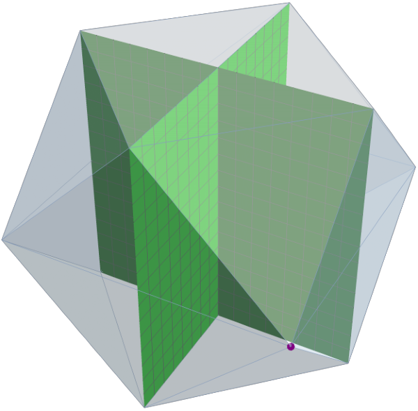
Note that, since this is the 3D-slice corresponding to $w=0$, the 4-tuple of correlations in question is the one specified above, namely $(w,x,y,z)=(0,1,-1,0)$.

7 The Bell real model, the CHSH inequalities, and Fine’s Theorem

The purpose of this section is to both derive the CHSH inequalities and prove Fine’s Theorem using the geometrically-motivated, parametric approach introduced in previous sections. The proof of the first result is childishly simple, and although the proof of the second result is a bit more work, once the machinery is set up, it is very compact. Specifically it is proved that

• $(\Rightarrow)$ If a model instance is Bell real, then it satisfies all 8 of the CHSH inequalities. Note this is then true for any Bell local model instance as well, since any Bell local model instance is also Bell real (Thm. 5). This “forward direction” is of course not new, being a generalization of Bell’s original inequalities, as proved in CHSH [17].

• $(\Leftarrow)$ Conversely, if a correlation vector satisfies the CHSH inequalities, then there exists a Bell real model instance that is consistent with the given correlations. Note that in some cases, there may be a Bell local model instance consistent with the given correlations, but not necessarily. Again, this “backward direction” result is not new, being essentially Fines’ Theorem [18]. However, the statement and proof of Thm. 7 is more in the spirit of Halliwell’s approach in [21] or Pitowski’s “correlation polytope” (Fig. 3) in [27].

7.1 Derivation of the CHSH inequalities

The forward direction (easy).

Theorem 6.

If a model instance is Bell real, then its correlations satisfy all 8 CHSH inequalities.

Proof.

Assume a Bell real model instance. See the $s$-functions sub-table in Table 13 of Sec. 5.3. Consider for example the $s_{1}$-function

$$2(\rho_{1}-\rho_{2}+\rho_{3}-\rho_{4}-\rho_{5}-\rho_{6}+\rho_{7}+\rho_{8}+\rho_{9}+\rho_{10}-\rho_{11}-\rho_{12}-\rho_{13}+\rho_{14}-\rho_{15}+\rho_{16}).$$

Since $\boldsymbol{\rho}=(\rho_{1},\rho_{2},...,\rho_{16})$ is a pmf, it is obvious that the $s_{1}$-function is between $-2$ and $+2$, hence two of the eight CHSH inequalities are satisfied. The same argument applies to the other three $s$-functions, so all eight CHSH inequalities are satisfied. ∎

7.2 Fine’s Theorem

The reverse direction (harder). It will be stated more precisely and proved after some definitions are made and two lemmas are stated and proved. They will make the proof go more smoothly, and will also add some geometric intuition.

Definition 27.

Define the 4D and 3D correlation vector regions, respectively, by $\mathcal{C}^{4}=\{\boldsymbol{p}\in R^{4}|-1\leq\boldsymbol{p}\leq 1\}$ and $\mathcal{C}^{3}=\{\boldsymbol{p}\in R^{3}|-1\leq\boldsymbol{p}\leq 1\}$.

Definition 28.

Define the 4D and 3D CHSH inequality vector regions, respectively, by $\mathcal{B}^{4}=\{\boldsymbol{p}\in\mathcal{C}^{4}|-2\leq S\boldsymbol{p}^{T}\leq 2\}$ and $\mathcal{B}^{3}_{w}=\{\boldsymbol{p}_{w}=(x,y,z)\in\mathcal{C}^{3}|-2\leq S(w,x,y,z)^{T}\leq 2\}$, for some fixed $-1\leq w\leq 1$.

Fig. 11 shows $\mathcal{B}_{w}^{3}$, for $w=-1,-\frac{1}{2},0,\frac{1}{2},1$, from left to right. The red dots indicate vertices. There are 4 vertices on the tetrahedrons (leftmost $w=-1$ and rightmost $w=+1$), and 12 vertices on each of the middle three polyhedra.

Figure 11: $\mathcal{B}_{w}^{3}$ for five different values $w=-1,-\frac{1}{2},0,\frac{1}{2},1$.

Definition 29.

The vertex matrix $V$ is defined in three different ways, depending on the value of $w$.

$$V=\left(\begin{array}[]{cccccccccccc}w&w&w&w&w&w&w&w&w&w&w&w\\ w&-1&1&-w&w&1&-1&-w&1&1&-1&-1\\ 1&-w&w&-1&-1&-w&w&1&-1&1&1&-1\\ 1&1&1&1&-1&-1&-1&-1&-w&w&-w&w\end{array}\right)$$

if $-1<w<1$,

$$V=\left(\begin{array}[]{cccccccccccc}-1&-1&-1&-1\\ -1&1&-1&1\\ 1&-1&-1&1\\ 1&1&-1&-1\end{array}\right)\mbox{if $w=-1$},$$

$$V=\left(\begin{array}[]{cccccccccccccccc}1&1&1&1\\ 1&-1&1&-1\\ 1&-1&-1&1\\ 1&1&-1&-1\end{array}\right)\mbox{if $w=+1$}.$$

The following lemma basically says that any correlation vector $\boldsymbol{p}=(w,x,y,z)$ which satisfies all eight CHSH inequalities can be written as a convex combination of the columns of $V$. Fig. 11 above lends some intuition by showing the 3D hyperplanes corresponding to certain fixed values of $w$.

Lemma 1.

Pick an arbitrary point $\boldsymbol{p}=(w,x,y,z)$ $\in$ $\mathcal{B}^{4}$. Then there exists a pmf $\boldsymbol{\lambda}$ such that $\boldsymbol{p}^{T}=(w,x,y,z)^{T}=V\boldsymbol{\lambda}^{T}$. If $V$ has 12 rows (i.e., $-1<w<1$), $\boldsymbol{\lambda}=\left(\lambda_{1},\lambda_{2},\lambda_{3},\lambda_{4},...,\lambda_{12}\right)$, and if it has 4 rows (i.e., $w=\pm 1$), $\boldsymbol{\lambda}=\left(\lambda_{1},\lambda_{2},\lambda_{3},\lambda_{4}\right)$.

Proof.

Start by ignoring the first row of $V$ and consider the last three rows only. The columns of the resulting sub-matrix represent the coordinates of the vertices of certain 3D volumes $\mathcal{B}_{w}^{3}$ defined by the CHSH inequalities. See examples in Fig. 11, where the red dots indicate the vertices. Since all of these volumes, for any $-1\leq w\leq 1$, are formed by the intersection of a finite number of closed half-spaces, the result is a closed, convex region. The particular (hyper)planes represented by the CHSH inequalities also make the region bounded. Invoking a theorem of Minkowski, an arbitrary point $\boldsymbol{p}_{w}=(x,y,z)$ inside any of these bounded, closed, convex regions can be written as a convex combination of the extreme points of the region, in this case, the vertices. That is, $\boldsymbol{p}_{w}^{T}=(x,y,z)^{T}=V(2,3,4)\boldsymbol{\lambda}^{T}$, for some appropriate vertex matrix $V$ (where $V(2,3,4)$ denotes the last three rows of $V$) and pmf $\boldsymbol{\lambda}$. Since $\boldsymbol{\lambda}$ is a pmf, $w=(w,w,\text{...},w)\boldsymbol{\lambda}^{T}$, so by inserting all $w$’s as the first row of $V(2,3,4)$ to make $V$, it is easily seen that $\boldsymbol{p}^{T}=(w,x,y,z)^{T}=V\boldsymbol{\lambda}^{T}$ as well. ∎

Definition 30.

The reality matrix $R$ turns a garden variety pmf $\boldsymbol{\rho}$ into a set of Bell real conditional probabilities $R\boldsymbol{\rho}^{T}$, as in the “Bell real” column of Table 6 in Sec 2.3.

$$R=\left(\begin{array}[]{cccccccccccccccc}1&1&0&0&1&1&0&0&0&0&0&0&0&0&0&0\\ 1&0&1&0&1&0&1&0&0&0&0&0&0&0&0&0\\ 1&1&0&0&0&0&0&0&1&1&0&0&0&0&0&0\\ 1&0&1&0&0&0&0&0&1&0&1&0&0&0&0&0\\ 0&0&1&1&0&0&1&1&0&0&0&0&0&0&0&0\\ 0&1&0&1&0&1&0&1&0&0&0&0&0&0&0&0\\ 0&0&1&1&0&0&0&0&0&0&1&1&0&0&0&0\\ 0&1&0&1&0&0&0&0&0&1&0&1&0&0&0&0\\ 0&0&0&0&0&0&0&0&1&1&0&0&1&1&0&0\\ 0&0&0&0&0&0&0&0&1&0&1&0&1&0&1&0\\ 0&0&0&0&1&1&0&0&0&0&0&0&1&1&0&0\\ 0&0&0&0&1&0&1&0&0&0&0&0&1&0&1&0\\ 0&0&0&0&0&0&0&0&0&0&1&1&0&0&1&1\\ 0&0&0&0&0&0&0&0&0&1&0&1&0&1&0&1\\ 0&0&0&0&0&0&1&1&0&0&0&0&0&0&1&1\\ 0&0&0&0&0&1&0&1&0&0&0&0&0&1&0&1\end{array}\right)$$

Definition 31.

The magic matrix $M$ is defined in three different ways, depending on the value of $w$. $M$ is a stochastic matrix, since the rows consist of non-negative numbers that sum to 1.

$$M=\left(\begin{array}[]{cccccccccccccccc}\frac{1+w}{2}&0&0&0&0&0&0&0&\frac{1-w}{2}&0&0&0&0&0&0&0\\ 0&0&0&0&0&\frac{1+w}{2}&0&0&\frac{1-w}{2}&0&0&0&0&0&0&0\\ \frac{1+w}{2}&0&0&0&0&0&0&0&0&0&0&0&0&\frac{1-w}{2}&0&0\\ 0&0&0&0&0&0&0&0&0&0&\frac{1+w}{2}&0&0&\frac{1-w}{2}&0&0\\ 0&0&0&0&0&0&0&0&0&0&0&\frac{1+w}{2}&\frac{1-w}{2}&0&0&0\\ 0&0&0&0&\frac{1+w}{2}&0&0&0&0&\frac{1-w}{2}&0&0&0&0&0&0\\ 0&\frac{1+w}{2}&0&0&0&0&0&0&0&0&0&0&\frac{1-w}{2}&0&0&0\\ 0&\frac{1+w}{2}&0&0&0&0&0&0&0&\frac{1-w}{2}&0&0&0&0&0&0\\ 0&0&0&0&0&0&0&0&0&0&0&\frac{1+w}{2}&0&\frac{1-w}{2}&0&0\\ \frac{1+w}{2}&0&0&0&0&0&0&0&0&\frac{1-w}{2}&0&0&0&0&0&0\\ 0&\frac{1+w}{2}&0&0&0&0&0&0&\frac{1-w}{2}&0&0&0&0&0&0&0\\ 0&0&0&0&0&0&0&0&0&0&\frac{1+w}{2}&0&\frac{1-w}{2}&0&0&0\end{array}\right)$$

if $-1<w<1,$

$$M=\left(\begin{array}[]{cccccccccccccccc}0&0&0&0&0&0&0&0&1&0&0&0&0&0&0&0\\ 0&0&0&0&0&0&0&0&0&0&0&0&0&1&0&0\\ 0&0&0&0&0&0&0&0&0&0&0&0&1&0&0&0\\ 0&0&0&0&0&0&0&0&0&1&0&0&0&0&0&0\end{array}\right)\mbox{if $w=-1$},$$

$$M=\left(\begin{array}[]{cccccccccccccccc}0&0&0&0&0&0&0&0&0&0&0&0&0&0&0&1\\ 0&0&0&0&0&0&0&0&0&0&1&0&0&0&0&0\\ 0&0&0&0&0&0&0&0&0&0&0&1&0&0&0&0\\ 0&0&0&0&0&0&0&0&0&0&0&0&0&0&1&0\end{array}\right)\mbox{if $w=+1$.}$$

Lemma 2.

$CRM^{T}=V$.

Proof.

This is a straightforward but tedious matrix multiplication, so it is left to the reader. There are three cases to consider depending on the value of $w$. Mathematica or other computational software platform is helpful here! ∎

Finally Fine’s Theorem can be stated and proved. The proof may be of interest due to its compactness and its basis in the geometry exemplified by the polyhedra shown in Fig. 11.

Theorem 7.

(Fine’s Theorem) Given an arbitrary correlation vector $\boldsymbol{p}=(w,x,y,z)$ that satisfies the CHSH inequalities. Let $\boldsymbol{\lambda}$ be a pmf such that $\boldsymbol{p}^{T}=V\boldsymbol{\lambda}^{T}$ as guaranteed by Lemma 1. Define

• $\boldsymbol{\rho}=(\rho_{1},\rho_{2},...,\rho_{16})=\boldsymbol{\lambda}M$,

• $\boldsymbol{\gamma}^{T}=(\gamma_{1},\gamma_{2},...,\gamma_{16})^{T}=R\boldsymbol{\rho}^{T}=RM^{T}\boldsymbol{\lambda}^{T}$.

Then

• $\boldsymbol{\rho}$ is a pmf and therefore $\boldsymbol{\gamma}$ is a set of Bell real conditional probabilities.

• The Bell real conditional probabilities $\boldsymbol{\gamma}$ are consistent with the correlations $\boldsymbol{p}$.

Proof.

For the first conclusion, note that $\boldsymbol{\rho}$ is a pmf because the rows of $M$ are pmf’s, $\boldsymbol{\lambda}$ is a pmf, therefore $\boldsymbol{\rho}=\boldsymbol{\lambda}M$, being a convex combination of pmf’s, is also a pmf. Thus $\boldsymbol{\gamma}^{T}=R\boldsymbol{\rho}^{T}$ is a set of Bell real conditional probabilities by the very definition of $R$.
For the second conclusion, invoke Lemma 2 to write

$$\boldsymbol{p}^{T}=V\boldsymbol{\lambda}^{T}=CRM^{T}\boldsymbol{\lambda}^{T}=C\boldsymbol{\gamma}^{T},$$

that is, the initial arbitrary correlation vector $\boldsymbol{p}$ that was assumed to satisfy the CHSH inequalities (i.e. is in $\mathcal{B}^{4}$) is equal to the computed correlations $C\boldsymbol{\gamma}^{T}$ based on the Bell real conditional probabilities $\boldsymbol{\gamma}$. ∎

7.3 What Fine’s Theorem does not say

Not every generic model instance that satisfies the CHSH inequalities is Bell real. Fine’s Theorem only guarantees that there exists some Bell real model instance with the same correlations as the given generic model instance. The mapping from model instances to correlation vectors is many-to-one! Consider the generic (maximal) predictable model with parameters $\boldsymbol{\gamma}=(1,1,1,0,0,0,0,0,0,0,0,0,0,\\ 0,0,1)$. The corresponding correlations are $(w,x,y,z)=(1,1,1,1)$ and the $s$-functions are $(s_{1},s_{2},s_{3},s_{4})=(2,2,2,2)$. However, it is fairly obvious that there is no pmf $\boldsymbol{\rho}$ such that

$$\left(\begin{array}[]{l}\rho_{1}+\rho_{2}+\rho_{5}+\rho_{6}\\ \rho_{1}+\rho_{3}+\rho_{5}+\rho_{7}\\ \rho_{1}+\rho_{2}+\rho_{9}+\rho_{10}\\ \rho_{1}+\rho_{3}+\rho_{9}+\rho_{11}\\ \rho_{3}+\rho_{4}+\rho_{7}+\rho_{8}\\ \rho_{2}+\rho_{4}+\rho_{6}+\rho_{8}\\ \rho_{3}+\rho_{4}+\rho_{11}+\rho_{12}\\ \rho_{2}+\rho_{4}+\rho_{10}+\rho_{12}\\ \rho_{9}+\rho_{10}+\rho_{13}+\rho_{14}\\ \rho_{9}+\rho_{11}+\rho_{13}+\rho_{15}\\ \rho_{5}+\rho_{6}+\rho_{13}+\rho_{14}\\ \rho_{5}+\rho_{7}+\rho_{13}+\rho_{15}\\ \rho_{11}+\rho_{12}+\rho_{15}+\rho_{16}\\ \rho_{10}+\rho_{12}+\rho_{14}+\rho_{16}\\ \rho_{7}+\rho_{8}+\rho_{15}+\rho_{16}\\ \rho_{6}+\rho_{8}+\rho_{14}+\rho_{16}\end{array}\right)=\left(\begin{array}[]{l}1\\ 1\\ 1\\ 0\\ 0\\ 0\\ 0\\ 0\\ 0\\ 0\\ 0\\ 0\\ 0\\ 0\\ 0\\ 1\end{array}\right).$$

Just start knocking off all of the $\rho_{k}$’s on the left in rows where 0’s appear in the column vector on the right, and pretty soon there is nothing left to make 1’s in rows 1,2,3, or 16.

7.4 Fine’s Theorem in action

Fig. 12 shows example output from a Mathematica interactive program that finds the Bell real pmf $\boldsymbol{\rho}$ that is consistent with a random set of correlations $\boldsymbol{p}$. Moving the slider selects different values for the first correlation $w$, and a triple of the remaining correlations $(x,y,z)$ is chosen randomly (constrained so that $(w,x,y,z)$ satisfies the CHSH inequalities, of course). Both the appropriate CHSH inequality region shape (as a 3D slice) and the random point $(x,y,z)$ are then displayed, along with tables of values showing, respectively from left to right, the coordinates of the random point $\boldsymbol{p}$, the computed correlations based on the Bell real conditional probabilities $\boldsymbol{\rho}$, whether or not they are equal, the coefficients of the point $\boldsymbol{p}$ as a convex combination of the vertices of the polyhedron, and finally the Bell real conditional probabilities $\boldsymbol{\rho}$ that were generated from $\boldsymbol{p}$’s coefficients.

Figure 12: Mathematica interactive demo for finding a pmf $\boldsymbol{\rho}$ consistent with a randomly chosen set of correlations $\boldsymbol{p}$ (purple dot). $w=0$ case is shown. Other cases are obtained by moving the slider in the control area at the top.

8 Relationships among Bell locality, FC, LC, RCI and ROI

8.1 Derivation of the form of the Bell local model

Define non-negative real numbers $\alpha_{1},\alpha_{2},\alpha_{3},\alpha_{4}$ and $\beta_{1},\beta_{2},\beta_{3},\beta_{4}$ by

$$\alpha_{1}=P(A=-1,D_{A}=-1),\;\beta_{1}=P(B=-1,D_{B}=-1),$$

$$\alpha_{3}=P(A=+1,D_{A}=-1),\;\beta_{3}=P(B=+1,D_{B}=-1),$$ (10)

$$\alpha_{2}=P(A=-1,D_{A}=+1),\;\beta_{2}=P(B=-1,D_{B}=+1),$$

$$\alpha_{4}=P(A=+1,D_{A}=+1),\;\beta_{4}=P(B=+1.D_{B}=+1).$$

Compare to Eq. 1 in Sec. 2.2.3. The only difference is that Eq. 1 expresses the $\alpha$’s and $\beta$’s in terms of the hidden r.v.’s and Eq. 10 gives them in terms of the operational r.v.’s. Table 23 shows the conditional probabilities $P(A|D_{A})$ and $P(B|D_{B})$ in terms of the $\alpha$’s and $\beta$’s (see columns 5 and 6). Finally, the last column imposes the factorization condition (FC – see Def. 9) by making every entry in column 7 equal to the product of the entries in columns 5 and 6 in the same row.

Table 23: Factorization condition defines the Bell local model.

Note that these match the conditional probabilities for the Bell local model as defined in Table 6 in Sec 2.3. The connection to Bell’s concept of locality as expressed in Bell [4] and as interpreted by Wiseman [36] can be found in Sec. 2.2. See also Shimony [31].

8.2 The special problem with LC and ROI

Consider the definitions of Bell local, FC, LC, RCI, and ROI in Sec. 2.2.2. Note that it is assumed that all of the relevant conditional probabilities must be well-defined for all values $(s,t,u,v)\in\{-1,1\}^{4}$. Now consider Table 24 showing probabilities conditioned on two and three r.v.’s, respectively (generic parameters only here).

Table 24: Probabilities conditioned on two and three r.v.’s (generic parameters)

The definitions of FC and RCI involve conditioning on at most two r.v.’s, so columns 5 and 6 indicate no problem in those cases (the reader should also check the case for conditioning on just one r.v.). However, it is clear from the final two columns of Table 24 that there could be an issue in confirming that a model instance is locally causal (LC) or satisfies remote outcome independence (ROI), since this involves conditioning on three r.v.’s. All of the denominators that appear in the entries of the final two columns must be non-zero.

A little bit of noodling in trying to meet this condition should convince the reader that a necessary condition is that at least 12 of the 16 parameters $\gamma_{1},\gamma_{2},...,\gamma_{16}$ must be greater than 0. In Table 25, the $x$’s indicate pairs of indices $(i,j)$ for which $\gamma_{i}+\gamma_{j}$ must be non-zero, because it appears as a denominator somewhere in Table 24. Now draw lines through as many columns (or alternatively rows) as are needed to “cover” all of the $x$’s. It should be fairly obvious that at least 12 such lines are required, hence at least 12 $\gamma_{k}$’s must be non-zero in order for an LC model instance to be legitimate. Note the same reasoning applies to any ROI model instance as well.

Table 25: Proof that at least 12 $\gamma_{k}$’s must be non-zero in any LC or ROI model instance.

8.3 FC implies RCI

Theorem 8.

If a model instance satisfies the factorization condition, then it satisfies the remote context independence (RCI) condition.

Proof.

Since a model satisfies FC iff it is Bell local, by the very definition of Bell local, it is sufficient to check whether or not a Bell local model satisfies RCI. Table 26 provides the evidence. ∎

Table 26: Proof of $FC\Rightarrow RCI$: Each of Alice’s and Bob’s outcomes depends only on her/his own detector setting.

8.4 LC is equivalent to RCI + ROI

In the interest of reducing clutter, in the next two subsections, the random variables will be suppressed, and only the corresponding values will be shown. For example,

$$P(A=s,B=t|D_{A}=u,D_{B}=v)\text{ will be shortened to }P(s,t|u,v)$$

for $(s,t,u,v)\in\{-1,1\}^{4}$. Also in the next two subsections, recall that, by the definitions of LC or ROI, conditional probabilities such as $P(s|t,u,v)$, $P(t|s,u,v)$, must be well-defined, that is, $P(s,u,v)>0$ and $P(t,u,v)>0$ (Def. 8 snd 11). Also $P(u,v)=P(D_{A}=u,D_{B}=v)>0$ must hold for all $(u,v)\in\{-1,1\}^{2}$ by the assumption that all detector pair-setting probabilities must be positive (Sec. 2).

Theorem 9.

A model instance is locally causal (LC) iff it satisfies both the remote context independent (RCI) condition and the remote outcome independence (ROI) condition.

Proof.

($\Rightarrow$) Assume LC. Then

$$P(s|u,v|t)=P(s|t,u,v)=P(s|u)$$ (11)

The first equality is the definition of iterated conditional probabilities and the second equality follows from LC. Then

$$P(s|u,v)=\sum_{t}P(s|u,v|t)P(t)=\sum_{t}P(s|u)P(t)=P(s|u)$$ (12)

The first equality follows from the law of total probability, the second equality follows from Eqn. 11, and the last equality from the fact that $\sum_{t}P(t)=1$. Similarly

$$P(t|u,v)=P(t|v)$$ (13)

Equations 12 and 13 show that any LC model instance satisfies RCI. So finally,

$$P(s|t,u,v)=P(s|u)=P(s|u,v)$$

$$P(t|s,u,v)=P(t|v)=P(t|u,v)$$ (14)

where the first equality in each line is from the definition of LC and the second equality in each line follows from RCI, as proved in equations 12 and 13.

($\Leftarrow$) Assume RCI and ROI. Then

$$P(s|t,u,v)=P(s|u,v)=P(s|u)$$

$$P(t|s,u,v)=P(t|u,v)=P(t|v)$$ (15)

where in each line, the first equality follows from ROI and the second equality follows from RCI. ∎

8.5 LC implies FC

Theorem 10.

If a model instance is locally causal (LC), then it also satisfies the factorization condition (FC).

Proof.

Assume LC. Then

$$P(s,t|u,v)=\frac{P(s,t,u,v)}{P(u,v)}=$$

$$\frac{P(s|t,u,v)P(t,u,v)}{P(u,v)}=\frac{P(s|u)P(t|u,v)P(u,v)}{P(u,v)}=$$ (16)

$$P(s|u)P(t|u,v)=P(s|u)P(t|v),$$

where the first line is by definition and the last two lines invoke a combination of the definitions of RCI and ROI, which is justified by Thm. 9. ∎

8.6 RCI does not imply LC by itself

Table 27 shows eight example parameter assignments that produce a generic (maximal) model that is RCI. Table 28 indicates the relevant conditional probabilities for Alice and Bob in model instance 1, clearly showing that RCI is satisfied. This is the same in all 8 cases.

Table 27: Eight Generic (Maximal) model instances

Table 28: Proof that the first generic model instance in Table 27 satisfies RCI: Each of Alice’s and Bob’s outcomes depends only on her/his own detector setting

Table 29: FC cannot hold in any of the 8 examples in Table 27 because one $s$-function is equal either to $+4$ or $-4.$

But none of these 8 instances can be Bell local, because in each case, one of the associated $s$-functions is either $-4$ or $+4$ (see Table 29). But if it is not Bell local, then it is not FC (by definition), and because it is not FC, it is not LC (by Thm. 10). QED

Note 10.

Since these examples violate CHSH (not to mention the Tsirelson bounds!), none of them can be Bell real, so they are examples of model instances that are RCI but not Bell real. See Sec. 10 for a proof that every Bell real model instance satisfies RCI. This explains the positioning of RCI strictly above Bell real in Fig. 3. It also explains why the box labeled “RCI” is outlined in green, since Table 29 shows examples that are RCI but also violate at least one Tsirelson bound.

It is interesting to compute the correlations associated with these 8 model instances, and situate them relative to the sets of correlations for the corresponding QM, Bell real, and Bell local models. See Table 30, which shows the correlations of these 8 examples, and take special note of the four correlation vectors in which $w=-1$ (cases 1,6,7,8). The corresponding four $(x,y,z)$ points are plotted as purple dots in Fig. 13. The tetrahedron in this figure is the Bell real region for $w=-1$. Note that the set of 4 purple vertices and the set of 4 red vertices form a partition of the the 8 vertices of the correlation cube.

This would still be true if either the QM or Bell local surfaces for $w=-1$ were to be substituted for the the Bell real region (see for example Fig. 7). It would also hold (in reverse) for the case $w=+1$. So in a certain sense, for the cases $w=\pm 1$, the correlations associated with these 8 examples of RCI (but not Bell real) are as far away as possible from being consistent with the corresponding QM, Bell real, or Bell local models.

Table 30: Correlations of the 8 examples that satisfy RCI but not FC.

Figure 13: $(x,y,z)$ correlations from RCI examples $1,6,7,8$ (purple dots) are the complement of the corresponding Bell real, Bell local, QM correlations (red dots). ($(-1,1,-1)$ (purple) is hidden).

8.7 ROI does not imply LC by itself

Table 31 shows an assignment of generic parameters $\gamma_{1},\gamma_{2},...,\gamma_{16}$, together with the associated correlations and $s$-functions. Note that $s_{3}=-2.6108$ (in red) violates the lower bound of $-2$ of the CHSH inequalities. Hence the model instance cannot be Bell local, hence cannot satisfy FC (by definition of Bell local), hence cannot satisfy LC (by Thm. 10).

Table 31: Example does not satisfy CHSH. Note $s_{3}=-2.6108<-2$ (in red).

However, Table 32 shows that this model instance satisfies ROI. This example explains the positioning of ROI strictly above LC (RCI and ROI) in Fig. 3.

Note 11.

The values in Table 32 have been rounded to 4 decimal places. If the reader attempts to check the claims, there may be some discrepancies. Mathematica returns the model parameters in exact integer format, which is too long to display here. If desired, contact the author to get the Mathematica-derived results.

Table 32: Example does satisfy ROI.

8.8 RCI and ROI are distinct

In Sec.’s 8.6 and 8.7 example model instances were shown that are, respectively,

• RCI but not LC and

• ROI but not LC.

These instances are obviously different, demonstrating that neither the set of RCI model instances nor the set of ROI model instances can contain the other. This fact is reflected by the positioning of the RCI and ROI nodes on different paths in Fig. 3.

9 Locality and the QM model

It will be shown in Sec. 11 that, in the “correlation equivalence” sense (Def. 32), there are QM model instances that are not Bell real and not Bell local (Sec. 11.5), and some that are Bell real but not Bell local (Sec. 11.4). In this section, the way in which a QM model instance can fail to be local is explored in more depth.

9.1 Some QM model instances do not satisfy FC

Consider the standard maximum deviation example where $\theta_{1}=67.5^{\circ},\theta_{2}=22.5^{\circ},\theta_{3}=22.5^{\circ},\theta_{4}=22.5^{\circ}$ produces $2\sqrt{2}$ for the $s_{1}$-function, for instance. The following Table 33 shows that in this special case, the QM model violates the factorization condition of Def. 9 in the worst possible way – the requirement $P(A,B|D_{A},D_{B})=P(A|D_{A})\times P(B|D_{B})$ fails for every assignment of values to $A,B,D_{A},D_{B}$.

Table 33: QM model instance that definitely does not satisfy the Factorization Condition (is not Bell local) when $\theta_{1}=67.5^{\circ},\theta_{2}=22.5^{\circ},\theta_{3}=22.5^{\circ},\theta_{4}=22.5^{\circ}$

9.2 QM model instances are generally RCI but not generally ROI

It is interesting to determine whether it is RCI or ROI (or both) that fails. Table 34 shows that RCI is satisfied in general, but Table 35 shows that ROI fails unless the measurement difference angles $\theta_{1},\theta_{2},\theta_{3},\theta_{4}$ are all of the form $\theta_{k}=(2j_{k}+1)\frac{\pi}{4}$ for integers $j_{k}$, which produces the trivial (minimal) model.

Table 34: QM model instances do satisfy RCI in general

Table 35: QM model instances do not satisfy ROI in general

10 Locality and the Bell real model

10.1 Some Bell real model instances do not satisfy FC

It has been shown in Thm. 5 that every Bell local model instance is also Bell real, and also that there exist Bell real model instances that are not Bell local. See Sec. 6.2 for an example. In the next section, the way in which a Bell real model instance can fail to be local is explored in more detail.

10.2 Bell real model instances are generally RCI but not generally ROI

Theorem 11.

If a model instance is Bell real, then it also satisfies RCI.

Proof.

See Tables 36 and 37. ∎

Table 36: Bell real model instances do satisfy RCI in general: Alice’s case.

Table 37: Bell real model instances do satisfy RCI in general: Bob’s case

To see that being Bell real but does not guarantee satisfaction of ROI, see Tables 38 and 39. The 32 equations (16 for Alice and 16 for Bob) that must be solved to satisfy ROI are precisely the conditions necessary for a Bell real model to be LC. In other words, adding the ROI condition to a Bell real model, which is already RCI (Tables 36 and 37), makes it LC. Since a Bell local model instance is defined by saying it satisfies FC, and it has been shown that $LC\Leftrightarrow RCI+ROI$ (Thm. 9) and $LC\Rightarrow FC$ (Thm. 10), this is not a surprise.

Table 38: Bell real model instances do not satisfy ROI in general (Alice outcomes)

Table 39: Bell real model instances do not satisfy ROI in general (Bob outcomes)

Note 12.

The QM model instances also generally satisfy RCI but not ROI, so in this sense of locality, QM and Bell real model types have a lot in common!

11 Correlation equivalence

In this section, the capability of two different model instances to produce the same set of correlations will be examined.

Definition 32.

Two model instances will be called correlation equivalent if the there is a correlation vector that is consistent with each instance, that is, the model instances can achieve a common set of correlations.

Definition 33.

Two model instances will be called equivalent if they have exactly the same generic parameters (conditional probabilities $P(A,B|D_{A},D_{B})$).

Note 13.

Obviously, if two model instances are equivalent, then they are also correlation equivalent, since correlations are simple linear functions of the generic parameters, i.e., $\mathbf{c}^{T}=C\mathbf{\gamma}^{T}$, where $C$ is the correlation matrix (see Def. 18).

Note 14.

In Sec. 6, it was shown that every Bell local model instance is equivalent to some Bell real model instance, hence every Bell local model instance is also correlation equivalent to some Bell real model instance.

11.1 Correlation equivalence “truth table”

One might ask: “Is there an example of a correlation vector that is consistent with some QM model instance and also with some Bell real model instance, but is not consistent with any Bell local model instance?”

All such questions are answered in the following Table 40, with pointers to at least one specific example, when the answer is “True”. For example, row 2 indicates that there is a positive answer to the question posed above, and to see example 2 below. The answer in rows 3 and 7 is “False” because there cannot be a correlation vector that is consistent with some Bell local model instance without also being consistent with some Bell real model instance, since every Bell local model instance is Bell real (Sec. 6).

Table 40: Truth table for correlation equivalence of QM, Bell real, and Bell local models, with examples

11.2 Examples 1: QM and Bell real and Bell local

Several examples are given here. The first example is the trivial one, namely the minimal model with all zero correlations.

Table 41: Parameter assignments for $(w,x,y,z)=(0,0,0,0)$.

Here is a more interesting example.

Table 42: Parameter assignments for $(w,x,y,z)=(-1,1,-1,1)$.

Finally, Fig. 14 shows an infinite number of examples for the QM and Bell local model types in the cases $w=-1$ and $w=0$ . The red lines indicate the intersection of the QM and Bell local correlations contours. Every point on these red lines corresponds to a 4-tuple of correlations $(-1,x,y,z)$ or $(0,x,y,z)$, respectively, where a Bell local model can achieve the corresponding QM correlations. The $s$-functions are therefore equal as well, and thus the CHSH inequalities are satisfied there. Note that each of these correlation vectors is automatically achievable by a Bell real model instance since every Bell local instance is also Bell real.

Figure 14: Red lines indicate correlations that are simultaneously achievable by QM and Bell local model instances (cases for $w=-1$ and $w=0$, respectively, are shown).

Table 43: Two specific examples of QM and Bell local model instance correlation equivalence, one for $w=-1$ and one for $w=0$.

A specific example point is shown on a red line in each plot (purple dots) . On the left ($w=-1$ case), the point $(\frac{2}{3},-1,\frac{2}{3})$ is shown and on the right ($w=0$ case), the point $(0,-\frac{1}{2},\frac{1}{2})$ is shown. The parameters for each model instance that give rise to this correlation equivalence are shown in Table 43.

11.3 QM and Bell local model equivalence

Despite the fact that there are an infinite number of correlation equivalent QM and Bell local model instances (see Sec 11.2), equivalence (Def. 33) is an entirely different matter. The only QM model instance equivalent to a Bell local model instance is the trivial (minimal) one. This can be easily seen as follows.

Consider Table 6 in Sec 2.3, columns 6 and 8 for the QM and Bell local models, respectively. After setting these two conditional probability vectors equal to each other, identities such as the following emerge:

$$\frac{1}{2}=\frac{1}{2}\cos^{2}(\theta_{1})+\frac{1}{2}\sin^{2}(\theta_{1})=\alpha_{1}\beta_{1}+\alpha_{1}\beta_{3}=\alpha_{1}(\beta_{1}+\beta_{3})=\alpha_{1}$$

Similarly, $\alpha_{k}=\beta_{k}=\frac{1}{2}$ for all $k=1,2,3,4$. In this case, all of the Bell local conditional probabilities $\alpha_{j}\beta_{k}$ are equal to $\frac{1}{4}$, and all of the correlations are zero. The QM parameter settings which achieve this same set of conditional probabilities (and correlations, of course) are $\theta_{1}=135^{\circ}\text{ and }\theta_{k}=45^{\circ}$ for $k=2,3,4$.

Table 44: QM and Bell local instances that achieve the correlations $(w,x,y,z)=(0,0,-\frac{1}{2},\frac{1}{2})$.

So what about the fact that there are non-trivial examples of QM and Bell local model instances that achieve the same correlations (an infinite number of them, in fact), as shown in Sec. 11.2? Again, the mapping from conditional probability parameters to correlations is many-to-one! Consider the two specific examples shown in Table 43, and despite the fact that in each case the correlations are the same, the generic parameters are quite different, as shown in Tables 44 and 45.

Table 45: QM and Bell local instances that achieve the correlations $(w,x,y,z)=(-1,\frac{2}{3},-1,\frac{2}{3})$.

11.4 Example 2: QM and Bell real and not Bell local

Table 46 shows the parameter assignments for the QM and Bell real models that are consistent with the correlations $(w,x,y,z)=(0,1,-1,0)$. The reason that there cannot be any Bell local model consistent with these correlations is given in Sec. 6.2.

Table 46: Parameter assignments for $(w,x,y,z)=(0,1,-1,0)$.

Note that just because a Bell real model instance has the same correlations as a given QM model (“correlation equivalent”), it does not mean that it is “equivalent” in the sense of having the same conditional probabilities. See Table 47. Both of the Bell real model instances (columns 3 and 4) reproduce the QM correlations of $(0,1,-1,0)$, but only the first one (column 3) has exactly the same conditional probabilities.

Table 47: Example of QM model instance and two distinct Bell real model instances that are consistent with the same set of correlations $(w,x,y,z)=(0,1,-1,0)$.

11.5 Example 3: QM and not Bell real and not Bell local

Pick the notorious set of angles for the QM model that produces the maximum violation of a bound in at least one of the CHSH inequalities (Table 48). There is no Bell real model instance consistent with these correlations because it must satisfy all 8 CHSH inequalities, and since any Bell local model instance is also Bell real, there can be no Bell local model instance consistent with them either.

Table 48: Parameter assignment for $(w,x,y,z)=1/2\sqrt{2}(-1,1,1,1)$.

11.6 Example 4: Not QM and Bell real and Bell local

Table 49 shows the Bell real and Bell local parameter assignments that achieve the correlations $(w,x,y,z)=(0,0,0,1)$. These correlations cannot be achieved by any QM model instance because it is necessary that, for some integers $k_{1},k_{2},k_{3},k_{4}$, $\theta_{1}=(2k_{1}+1)\frac{\pi}{4}$, $\theta_{2}=(2k_{2}+1)\frac{\pi}{4}$, $\theta_{3}=(2k_{3}+1)\frac{\pi}{4}$, and $\theta_{4}=k_{4}\pi$. Then $\theta_{1}=\theta_{2}+\theta_{3}+\theta_{4}$ reduces to $2\left(k_{1}-k_{2}-k_{3}-2k_{4}\right)=1$, a contradiction. QED. Fig. 15 illustrates what has just been proved.

Table 49: Parameter assignments for $(w,x,y,z)=(0,0,0,1)$.

Figure 15: Correlations $(w,x,y,z)=(0,0,0,1)$ achievable by Bell real and Bell local models but not by any QM model (purple dot in middle of top square).

11.7 Example 5: Not QM and Bell real and not Bell local

Table 50 shows a Bell real parameter assignment that achieves the correlations $(w,x,y,z)=(-1,-\frac{1}{3},-\frac{1}{3},\frac{1}{3})$.

Table 50: Parameter assignment for $(w,x,y,z)=(-1,-\frac{1}{3},-\frac{1}{3},\frac{1}{3})$.

However, $(-1,-\frac{1}{3},-\frac{1}{3},\frac{1}{3})$ cannot be achieved by any assignment of parameters to a Bell local model. Consider the equations that must be solved:

$$\left(\begin{array}[]{l}(\alpha_{1}-\alpha_{3})(\beta_{1}-\beta_{3})\\ (\alpha_{1}-\alpha_{3})(\beta_{2}-\beta_{4})\\ (\alpha_{2}-\alpha_{4})(\beta_{1}-\beta_{3})\\ (\alpha_{2}-\alpha_{4})(\beta_{2}-\beta_{4})\\ \end{array}\right)=\left(\begin{array}[]{c}-1\\ -\frac{1}{3}\\ -\frac{1}{3}\\ \frac{1}{3}\\ \end{array}\right).$$

To make the first term $-1$, set $\alpha_{1}=\beta_{3}=1$ and $\alpha_{3}=\beta_{1}=0$ OR $\alpha_{1}=\beta_{3}=0$ and $\alpha_{3}=\beta_{1}=1$. Suppose the first choice is made. Then to make the second and third terms equal to $-\frac{1}{3}$, it is necessary to set $\alpha_{4}=\beta_{2}=\frac{1}{3}$ and $\alpha_{2}=\beta_{4}=\frac{2}{3}$. But then the last term will be $-\frac{1}{9}$ instead of $\frac{1}{3}$, as required. A similar contradiction results from the other choice $\alpha_{1}=\beta_{3}=0$ and $\alpha_{3}=\beta_{1}=1$.
This correlation vector also cannot be achieved by any QM model instance. For let $x=\frac{1}{2}\arccos{(-\frac{1}{3})}$. Then it is necessary that, for some integers $k_{1},k_{2},k_{3},k_{4}$, $\theta_{1}=\left(2k_{1}+1\right)\frac{\pi}{2}$, $\theta_{2}=x+k_{2}\pi$, $\theta_{3}=x+k_{3}\pi$, and $\theta_{4}=-x+(2k_{4}+1)\frac{\pi}{2}$, so $\theta_{1}=\theta_{2}+\theta_{3}+\theta_{4}$ reduces to $2\left(k_{1}-k_{2}-k_{3}-k_{4}\right)=1+\frac{2x}{\pi}$, which equates an integer to a non-integer, a contradiction. QED. Fig. 16 illustrates what has just been proved.

Figure 16: Correlations $(w,x,y,z)=(-1,-\frac{1}{3},-\frac{1}{3},\frac{1}{3})$ for not QM, Bell real, not Bell local (blue dot in middle of triangular face).

11.8 Example 6: Not QM and not Bell real and not Bell local

See Fig. 15 in Sec. 11.6, and notice the point $(1,-1,-1)$ (black dot at the bottom front) corresponding to the correlations $(w,x,y,z)=(0,1,-1,-1)$ . It is not in the Bell region because not all of the CHSH inequalities are satisfied; the second $s$-function has value $s_{2}=-3<-2$. Since it is not in the Bell region, it also cannot be on the Bell local contour either.

This correlation vector also cannot be achieved by any QM model since $\theta_{1}$ would have to be of the form $(2k_{1}+1)\frac{\pi}{4}$, $\theta_{2}$ of the form $k_{2}\pi$, $\theta_{3}$ of the form $(2k_{3}+1)\frac{\pi}{2}$, and $\theta_{4}$ of the form $(2k_{4}+1)\frac{\pi}{2}$, so $\theta_{1}=\theta_{2}+\theta_{3}+\theta_{4}$ reduces to $2(k_{1}-2k_{2}-2k_{3}-2k_{4})=3$, a contradiction. QED

12 Bell’s theorem using achievable correlations

This section contrasts the traditional inequality-based Bell’s theorem with an approach based on achievable correlations. Fig. 17 is an illustration of the traditional inequality-based approach. The green square represents one of the CHSH inequality bounds (2), and the yellow surface represents the QM $s_{1}$-function, as a function of the two free parameters $\theta_{3}$ and $\theta_{4}$, based on the two constraints $\theta_{1}=\theta_{2}+\theta_{3}+\theta_{4}$ and $\theta_{2}=22.5^{\circ}$. The small hill above the green square indicates where the CHSH inequality is violated. The purple dot at the top of the hill shows the maximum deviation of $2\sqrt{2}$ when $\theta_{2}=\theta_{3}=\theta_{4}=22.5^{\circ}$ and $\theta_{1}=67.5^{\circ}$.

Figure 17: Illustration of the violation of one of the CHSH inequalities by the $s_{1}$-function of QM correlations ($\theta_{2}=22.5^{\circ}$ is held fixed).

Now consider the graphs of different model type correlations in Fig. 6 in Sec. 4.1. These pictures suggest very strongly that QM model instances can be differentiated from other types of model instances based on achievable correlations alone. The following theorem provides a simple way to distinguish non-QM model instances from QM ones.

Theorem 12.

Given a generic model instance $\mathcal{G}$. Then necessary and sufficient conditions for $\mathcal{G}$ to be a QM model instance with parameters $(\theta_{1},\theta_{2},\theta_{3},\theta_{4})$ (where $\theta_{1}=\theta_{2}+\theta_{3}+\theta_{4}$) are:

$$1.\>(w,x,y,z)=(\cos 2\theta_{1},\cos 2\theta_{2},\cos 2\theta_{3},\cos 2\theta_{4})$$

$$2.\>P(A=s|D_{A}=u)=P(B=t|D_{B}=v)=\frac{1}{2}\text{ for all }(s,t,u,v)\in\{-1,1\}^{4}.$$

Proof.

For necessity, see Table 10 in Sec. 5.2 for condition 1, and Table 34 in Sec. 9.2 for condition 2. As for sufficiency, confine the argument to the first generic correlation $w=\gamma_{1}-\gamma_{5}-\gamma_{9}+\gamma_{13}$. The same argument can be applied separately to the other three generic correlations

$$x=\gamma_{2}-\gamma_{6}-\gamma_{10}+\gamma_{14},$$

$$y=\gamma_{3}-\gamma_{7}-\gamma_{11}+\gamma_{15},$$

$$z=\gamma_{4}-\gamma_{8}-\gamma_{12}+\gamma_{16}.$$

since the four subsets of generic parameters are mutually disjoint. Setting the first generic correlation equal to the first QM correlation yields

$$\gamma_{1}-\gamma_{5}-\gamma_{9}+\gamma_{13}=\cos 2\theta_{1}=\cos^{2}\theta_{1}-\sin^{2}\theta_{1}.$$ (17)

Since by the definition of the generic model (see Table 1),

$$\gamma_{1}+\gamma_{5}+\gamma_{9}+\gamma_{13}=1,$$

it follows that

$$\gamma_{1}+\gamma_{13}=\cos^{2}\theta_{1}\text{ and }\gamma_{5}+\gamma_{9}=\sin^{2}\theta_{1}.$$ (18)

Now consult Table 51, which shows the generic forms of Alice’s and Bob’s conditional outcome probabilities given their own detector settings (last two columns, respectively). According to QM, these entries must all be $\frac{1}{2}$. Applying this requirement to the first entry in Alice’s column yields

$$\frac{(\gamma_{1}+\gamma_{5})\delta_{ab}+(\gamma_{2}+\gamma_{6})\delta_{ab^{\prime}}}{\delta_{ab}+\delta_{ab^{\prime}}}=\frac{1}{2}.$$

Since this must be true no matter the detector-setting probabilities $\delta_{ab},\delta_{ab^{\prime}}$ (because the actual experimental detector-setting frequencies may vary), it follows that $\gamma_{1}+\gamma_{5}=\gamma_{2}+\gamma_{6}=\frac{1}{2}$.

Table 51: Generic conditional probabilities that must be equal to 1/2 to mimic a QM model.

This must be true for all terms in Table 51 of the form $(\gamma_{i}+\gamma_{j})$, so in particular

$$\gamma_{1}+\gamma_{5}=\gamma_{9}+\gamma_{13}=\gamma_{1}+\gamma_{9}=\gamma_{5}+\gamma_{13}=\frac{1}{2},$$ (19)

since these sums appear somewhere in the table. Subtracting the last term from the first in Eq. 19 yields $\gamma_{1}=\gamma_{13}$ and and subtracting the third from the first yields $\gamma_{5}=\gamma_{9}$. Combining with Eq. 18 immediately yields

$$\gamma_{1}=\frac{1}{2}\cos^{2}\theta_{1}\text{ and }\gamma_{5}=\frac{1}{2}\sin^{2}\theta_{1},$$ (20)

$$\gamma_{9}=\frac{1}{2}\sin^{2}\theta_{1}\text{ and }\gamma_{13}=\frac{1}{2}\cos^{2}\theta_{1}.$$

The end result, after repeating this argument for the other three correlations, is that

$$\boldsymbol{\gamma}=(\gamma_{1},\gamma_{2},\gamma_{3},\gamma_{4},\gamma_{5},\gamma_{6},\gamma_{7},\gamma_{8},\gamma_{9},\gamma_{10},\gamma_{11},\gamma_{12},\gamma_{13},\gamma_{14},\gamma_{15},\gamma_{16})=$$ (21)

$$\frac{1}{2}(\cos^{2}\theta_{1},\cos^{2}\theta_{2},\cos^{2}\theta_{3},\cos^{2}\theta_{4},\sin^{2}\theta_{1},\sin^{2}\theta_{2},\sin^{2}\theta_{3},\sin^{2}\theta_{4},...,\cos^{2}\theta_{3},\cos^{2}\theta_{4}),$$

that is, any generic model instance that has the same correlations as a QM model instance, and satisfies the requirement that the conditional probabilities $P(A|D_{A})=P(B|D_{B})=\frac{1}{2}$, must be a QM model instance. ∎

This enables very simple proofs, without inequalities, that certain model types cannot replicate all QM model behaviors. For example, it is trivial to show that the only generic model instance that is both QM and Bell local is the trivial (minimal) model instance. In fact, only the second condition of Thm. 12 is required. That is, it requires that all of the parameters of the Bell local model be equal to $\frac{1}{2}$;

$$\alpha_{1}=\alpha_{2}=\alpha_{3}=\alpha_{4}=\frac{1}{2},$$

$$\beta_{1}=\beta_{2}=\beta_{3}=\beta_{4}=\frac{1}{2}.$$

But then all of the conditional probabilities $P(A,B|D_{A},D_{B})$ of this Bell local model are equal to $\frac{1}{4}$:

$$\alpha_{1}\beta_{1}=\alpha_{1}\beta_{2}=...=\alpha_{4}\beta_{4}=\frac{1}{4},$$

which is the definition of the trivial (minimal) model. See Table 6 in Sec 2.3.

13 Final summary

The mathematical gist of this paper is:

1. Assumptions

   • A set of 4 operational r.v.’s: Alice’s and Bob’s two outcomes and two detector settings,

   • A set of “hidden” r.v.’s with an associated pmf,

   • A complete, joint pmf on the combined set of operational and hidden r.v.’s such that the marginal pmf of the hidden r.v.’s is the same as the original given one.

2. Analysis

   • Marginalize the combined pmf to a pmf on the operational r.v.’s only. Call this pmf “generic”,

   • Define specific flavors of the generic pmf to represent

     • Local hidden variables (Bell real),

     • The factorization condition (Bell local),

     • Predictability,

     • Local causality,

     • Remote context independence,

     • Remote outcome independence

     .

3. Conclusions

   • Some Bell real or Bell local or predictable model instances can produce some QM correlations, but none can recreate all QM correlations.

The following list highlights a few results from this paper that either address certain misconceptions about Bell’s Theorem and/or may not be well known or appreciated. For a complete summary of the results, see Sec. 3.

• QM correlations just look different. Revisit Fig.’s 6 and 7 in Sec.’s 4.1 and 4.2. Note how different the QM correlations (first row in each table) look compared to the correlations in any other model row. This shows more than a simple inequality, or set of inequalities, how difficult it is to reproduce certain features of QM model instances using only assumptions of reality, locality, and/or predictability.

• However, QM and Bell real model instances have something in common.
  They share the properties of generally satisfying RCI, but not generally satisfying ROI. One often reads that quantum mechanics is “non-local”, but not so when it comes to RCI. In the context of an EPRB-like experiment, QM’s “non-localness” is tied up more with the outcomes than with the detector settings.

• “Local realism” is tricky. It is often stated in the literature that local realism is the basis of Bell’s inequality, seeming to imply that locality and realism are separate conditions and their conjunction is required to derive the CHSH inequalities. However, it is a little more nuanced than that.

  • First of all, the proof of Thm. 6 (Sec. 7.1) shows that it is enough to assume a model instance to be Bell real in order to get all 8 CHSH inequalities. “Locality”, in the form of remote context independence (RCI), comes along for the ride according to Thm. 11 in Sec. 10.2. On the other hand, one could take the position that RCI is already “built into” the definition of Bell real via the assumptions on the hidden variables that lead to its form (see Sec. 2.2). If so, the interpretation of conjoined “local” and “real” characteristics makes sense.

  • Second of all, if the “local” in “local realism” refers to “Bell local” , meaning a model instance satisfies the factorization condition (FC), than this assumption alone is sufficient to derive the CHSH inequalities, since every Bell local instance is also Bell real (Thm. 5 in Sec. 6). Again one could adopt the viewpoint that the hidden variables approach to defining “Bell real” and “Bell local” types already has reality and locality built into the Bell local model type since it is just a special case of the Bell real model type.

• Fine’s Theorem: Handle with care. It is worth emphasizing what Fine’s Theorem (Thm. 7) does and does not say. First, it says that if the CHSH inequalities hold for the correlations of some generic model instance, then there exists a Bell real model instance that achieves these correlations. But it does not say that any given generic model instance that satisfies all 8 CHSH inequalities is Bell real. A counterexample is given in Sec. 7.3. Put another way, one cannot say that the CHSH inequalities being satisfied by some generic model instance is sufficient evidence to declare the model instance to be Bell real, i.e., to be worthy of the name “real”.

• Predictable instances are special. See Fig.’s 3 and 5 in Sec. 3.

  • There are only a finite number of them (256).

  • Except for Type 1, they don’t “connect” to anybody except themselves (see Fig. 2 or 3)

  • Given a predictable model instance, it either:

    • Satisfies the CHSH inequalities (underachieves) as in Types 1 and 2, or

    • Exceeds the Tsirelson bounds (overachieves) as in Type 3 (but not 1 or 2).

References

- [1] Alain Aspect. Bell’s Theorem: The Naive View of an Experimentalist, “Quantum [Un]speakables From Bell to Quantum information”, edited by R. A. Bertlmann and A. Zeilinger, Springer, 2002.
- [2] John S. Bell. On the Einstein, Podolsky, Rosen Paradox, Physics Vol. 1, No. 3, pp. 195-290, 1964. (Reproduced in [11].)
- [3] John S. Bell. On the Problem of Hidden Variables in Quantum Mechanics Review of Modern Physics 38, 1976 (Reproduced in [11].)
- [4] John S. Bell. The Theory of Local Beables, Epistemological Letters 9, 1976; Dialectia 39 1985. (Reproduced in [11].)
- [5] John S. Bell. Bertlmann’s Socks and the Nature of Reality, Journal de Physique Colloques C2 Supplement 3, 1981. (Reproduced in [11].)
- [6] John S. Bell, EPR correlations and EPW distributions, New Techniques and Ideas in Quantum Measurement Theory, D. M. Greenberger,ed., Ann. New York Acad. Sci vol 480, 1986. (Reproduced in [11].)
- [7] John S. Bell. Introduction to the Hidden Variable Question,Proceedings of the International School of Physics ’Enrico Fermi’, course II: Foundations of Quantum Mechanics, Academic 171-81. New York, 1971.
- [8] John S. Bell. Speakable and Unspeakable in Quantum Mechanics: Collected Papers on Quantum Philosophy, Cambridge University Press, 1987.
- [9] John S. Bell. La nouvelle cuisine, Between Science and Technology , A Sarmeljin, P. Kroes, ed., Elsevier/North-Holland 1990. (Reproduced in [11].)
- [10] John S. Bell and M. Nauenberg, The moral aspects of quantum mechanics, Preludes in Theoretical Physics – In Honor of V.F. Weisskopf, de Shalit A, Feshbach H and van Hove L eds. Amsterdam: North Holland, 1966. (Reproduced in [11].)
- [11] John S. Bell. John S. Bell on the Foundations of Quantum Mechanics, M. Bell, K. Gottfried, M. Veltman, eds., World Scientific, Singapore, 2001.
- [12] Mary Bell and Shan Gao, ed.’s, Quantum Nonlocality and Reality: 50 Years of Bell’s Theorem, Cambridge University Press, 2016.
- [13] John S. Bell Google Scholar citations. https://scholar.google.com/citations?user=Bd9KX0oAAAAJ&hl=en#d=gsc_hist&p=&u=.
- [14] Jean Bricmont. What did Bell really prove? Quantum Non-Locality and Reality, M. Bell and S. Gao, ed., Cambridge University Press, 2016 – p. 49
- [15] Harvey R Brown, Christopher G Timpson. Bell on Bell’s Theorem: The Changing Face of Non-Locality, Quantum Non-Locality and Reality, M. Bell and S. Gao, ed., Cambridge University Press, 2016 – p.91.
- [16] Eric G. Cavalcanti and Howard M. Wiseman. Bell nonlocality, signal locality and upredictability (or What Bohr could have told Einstein at Solvay had he known about Bell experiments), arXiv:0911.2504v2 [quant-ph] 13 Jun 2012.
- [17] J.F. Clauser, M.A. Horne, A. Shimony, R.A. Holt. Proposed experiment to test local hidden-variable theories, Phys. Rev. Lett., 23 (15): 8804, Bibcode:1969PhRvL..23..880C, doi:10.1103/PhysRevLett.23.880), 1969.
- [18] Arthur Fine. Hidden Variables, Joint Probability, and the Bell Inequalities, Phys. Rev. Lett. 48, 291, February 1982.
- [19] Arthur Fine. The Einstein-Podolsky-Rosen Argument in Quantum Theory, The Stanford Encyclopedia of Philosophy, https://plato.stanford.edu/entries/qt-epr/#SpinBohmVers, First published Mon May 10, 2004; substantive revision Tue Oct 31, 2017.
- [20] A. Gleason. Measures on closed subspaces of Hilbert space, Journal of Mathematics and Mechanics, 6, pp 885-893, 1957.
- [21] J.J.Halliwell. Two Proofs of Fine’s Theorem, arXiv.org$>$quant-ph$>$arXiv:1403.7136v2, April 2014.
- [22] Karl Hess, Hans De Raedt, Kristel Michielsen. Counterfactual Definiteness and Bell’s Inequality, arXiv:1605.04889v1 [quant-ph] 16 May 2016.
- [23] Karl Hess, Walter Philipp. The Bell Theorem as a Special Case of Bass, arXiv:quant-ph/0503044v1 3 Mar 2005.
- [24] J. P. Jarrett On the physical significance of the locality conditions in the Bell arguments, Nous, 18: 569–589, 1984.
- [25] Tim Maudlin. What Bell Did, J. Phys. A: Math. Theor. 47, 424010 (24pp), doi:10.1088/1751-8113/47/42/424010, 2014.
- [26] Tim Maudlin. What Bell Did, YouTube, https://www.youtube.com/watch?v=Vg5z/zeZP60, 2014.
- [27] I. Pitowski. Quantum Mechanics as a Theory of Probability, http://philsci-archive.pitt.edu/2474/1/TOBUB1.pdf, Oct 2005.
- [28] E. Rosinger. George Boole and the Bell Inequalities, arXiv.orgquant-ph/0406004v1, https://arxiv.org/abs/quant-ph/0406004, Jun 2004.
- [29] Benjamin Schumacher and Michael Westmoreland. Quantum Processes and Information, Cambridge University Press, 2010.
- [30] Abner Shimony. Contextual Hidden Variable Theories and Bell’s Inequalities, British Journal of the Philosophy of Science, pp 25-45, 1984.
- [31] Abner Shimony. Bell’s Theorem, The Stanford Encyclopedia of Philosophy, https://plato.stanford.edu/entries/bell-theorem/, First published Wed Jul 21, 2004; substantive revision Wed Mar 13, 2019.
- [32] Henry P. Stapp. “Strengthening Bell’s Theorem: Removing the Hidden-Variable Assumption”, Quantum Non-Locality and Reality, M. Bell and S. Gao, ed., Cambridge University Press, 2016 – p.151
- [33] Roderich Tumulka. What did Bell really prove?, Quantum Non-Locality and Reality, M. Bell and S. Gao, ed., Cambridge University Press, 2016 – p. 79
- [34] N. N. Vorobev. Consistent Families of Measures, “Theory of Probabilities and its Applications”, Volume VII, Number 2 1962.
- [35] Wikipedia. EPR Paradox https:en.wikipedia.org/wiki/EPR_paradox, 2017.
- [36] Howard Wiseman. The Two Bell’s Theorems of John Bell, arXiv:1402.0351v1 [quant-ph] 3 Feb 2014.