Nonparametric Continuous Sensor RegistrationThanks: W. Clark and A. Bloch are with Department of Mathematics, University of Michigan, Ann Arbor, MI 48109 USA {wiclark, abloch}@umich.eduThanks: M. Ghaffari is with College of Engineering, University of Michigan, Ann Arbor, MI 48109 USA {maanigj}@umich.edu

Abstract

This paper develops a new mathematical framework that enables nonparametric joint semantic/appearance and geometric representation of continuous functions using data. The joint semantic and geometric embedding is modeled by representing the processes in a reproducing kernel Hilbert space. The framework allows the functions to be defined on arbitrary smooth manifolds where the action of a Lie group is used to align them. The continuous functions allow the registration to be independent of a specific signal resolution and the framework is fully analytical with a closed-form derivation of the Riemannian gradient and Hessian. We study a more specialized but widely used case where the Lie group acts on functions isometrically. We solve the problem by maximizing the inner product between two functions defined over data, while the continuous action of the rigid body motion Lie group is captured through the integration of the flow in the corresponding Lie algebra. Low-dimensional cases are derived with numerical examples to show the generality of the proposed framework. The high-dimensional derivation for the special Euclidean group acting on the Euclidean space showcases the point cloud registration and bird’s-eye view map registration abilities. A specific derivation and implementation of this framework for RGB-D cameras outperform the state-of-the-art robust visual odometry and performs well in texture and structure-scares environments.

I Introduction

We consider the problem of sensor registration, which is defined as finding the transformation between two sensors with overlapping measurements or tracking a moving sensor using its sequential measurements. This problem frequently arises in engineering domains such as point cloud registration [1, 2, 3, 4, 5, 6, 7, 8], visual odometry and SLAM [9, 10, 11, 12, 13, 14, 15, 16], satellite image registration [17, 18], and photogrammetry [19]. In terms of applications, the above mentioned problems are fundamental to many computer vision [20, 21] and robotics [22, 23] algorithms.

The standard solution to sensor registration is typically formulated as a maximum likelihood or least-squares problem and solved via numerical optimization techniques. In the maximum likelihood setting, the measurement noise distribution significantly affects the robustness of the solver to outliers. Hence, in practice, the problem is necessarily solved using a robust estimator such as the iteratively reweighted least-squares algorithm or truncated least squares [24]. The central shortcoming of this approach is the reliance on point-wise correspondences between two measurement sets. As a result, the implicit assumption is that the perceived data points by digital sensors are from the same points in reality. Of course, this is seldom true as the nature of digital sensing means a discretization of the reality is captured at best. Sparse and uniform (feature-scarce) measurement sets are where this shortcoming can become problematic. A prime example is the lack of robustness of the visual odometry algorithms to texture and structure-less scenes.

In this paper, we formulate a fundamentally novel nonparametric framework for sensor registration that constructs continuous functions from measurements. The functions can be thought of as curves, surfaces, or hyper-surfaces that live in a Reproducing Kernel Hilbert Space (RKHS). For example, given an RGB-D image, a function can be constructed that maps a three-dimensional (3D) point to the RGB color space. Therefore, such functions inherently represent a joint model for semantic/appearance and geometry. Furthermore, the domain of the functions can be an arbitrary smooth manifold where the action of a Lie group is used to align them. This concept is illustrated in Figure 1. The continuous functions allow the registration to be independent of a specific signal resolution and the framework is fully analytical with a closed-form derivation of the Riemannian gradient and Hessian.

Figure 1: Conceptual illustration of nonparametric continuous sensor registration. Continuous functions are constructed from measurements shown in red circles. The domain of the functions can be an arbitrary smooth manifold, $M$, where the action of a Lie group, $\mathcal{G}$, is used to align them via $h.f_{Z}$ and $h\in\mathcal{G}$.

In the present work, we study a restriction of the framework where the Lie group acts on functions isometrically. This restriction has a variety of applications and its high-dimensional derivation for the special Euclidean group acting on the Euclidean space showcases the point cloud registration and bird’s-eye view map registration abilities. In particular, this work has the following contributions:

1. a new mathematical framework for sensor registration that enables nonparametric joint semantic/appearance and geometric representation of continuous functions using data;

2. low-dimensional cases are derived with numerical examples to show the generality of the proposed framework;

3. a high-dimensional derivation for the special Euclidean group acting on the Euclidean space showcases the point cloud registration and bird’s-eye view map registration abilities. A specific derivation and implementation of this framework for RGB-D cameras performs well in texture and structure-scarce environments.

4. the open-source implementation of the derived cases in this work is available for download at
   https://github.com/MaaniGhaffari/c-sensor-registration

The remainder of this paper is organized as follows. A review of the required mathematical machinery and notation is given in next section. Section III presents the novel continuous sensor registration framework. Section IV provides low-dimensional examples of the framework including point cloud registration on circles and torus. The high-dimensional example for the special Euclidean group is given in Section V. A brief theoretical analysis for the verification of the idea is provided in Section VI. The integration of the flow for $\mathrm{SE}(n)$ and for the 2D and 3D cases to obtain the solution is explained in Section VII. Section VIII deals with the Riemannian geometry of the special Euclidean groups. Experimental evaluations of the proposed method for registration and tracking using RGB-D images are presented in Section IX. Section X provides a discussion regarding the locality of solutions. Section XI shows the relationships between nonparametric continuous sensor registration and weighted least squares. Finally, Section XII concludes the paper and provides future work ideas.

II Required Mathematical Machinery and Notation

We first review some mathematical preliminaries to establish the notation and give the paper better flow before stating the main results.

II-A Matrix Lie Group of Motion in $\mathbb{R}^{n}$

The general linear group of degree $n$, denoted $\mathrm{GL}_{n}(\mathbb{R})$, is the set of all $n\times n$ real invertible matrices, where the group binary operation is the ordinary matrix multiplication. The $n$-dimensional special orthogonal group, denoted

$$\begin{split}\mathrm{SO}(n)=\{{R}\in\mathrm{GL}_{n}(\mathbb{R})|\penalty\ {R}{R}^{\mathsf{T}}={I}_{n},\operatorname{det}{R}=+1\},\end{split}$$

is the rotation group on $\mathbb{R}^{n}$. The $n$-dimensional special Euclidean group, denoted

$$\begin{split}\resizebox{22609920}{}{$\mathrm{SE}(n)=\left\{{h}=\left[\begin{array}[]{cc}{R}&{T}\\ 0&1\end{array}\right]\in\mathrm{GL}_{n+1}(\mathbb{R})|\penalty\ {R}\in\mathrm{SO}(n),{p}\in\mathbb{R}^{n}\right\},$}\end{split}$$

is the group of rigid transformations, i.e., direct isometries, on $\mathbb{R}^{n}$. A transformation such as ${h}\in\mathrm{SE}(3)$ is the parameter space in many sensor registration problems which consists of a rotation and a translation components. Let $\bar{{h}}\in\mathrm{SE}(3)$ be an estimate of ${h}$. We compute the rotational and translational distances using $\lVert{\log(\bar{{R}}{R}^{\mathsf{T}})}\rVert_{\mathrm{F}}$ and $\lVert{\bar{{T}}-\bar{{R}}{R}^{\mathsf{T}}{T}}\rVert$, respectively, where $\log(\cdot)$ is the Lie logarithm map which is, here, the matrix logarithm. These definitions are consistent with the transformation distance that can be directly computed using $\lVert{\log(\bar{{h}}{h}^{-1})}\rVert_{\mathrm{F}}$. Here, $\lVert A\rVert^{2}_{\mathrm{F}}=\tr(A^{\mathsf{T}}A)$ is the Frobenius norm.

This paper studies not only matrix Lie groups, but also their actions on manifolds. We have the following definition:

Definition 1.

Let $\mathcal{G}$ be a group and $X$ a set. A (left) group action of $\mathcal{G}$ on $X$, denoted as $\mathcal{G}\curvearrowright X$, is a group homomorphism $\mathcal{G}\to\emph{Aut}(X)$ (automorphism of $X$). If $X$ is a smooth manifold, the action is smooth if $\mathcal{G}\to\diff(X)$ (diffeomorphism of $X$).

Remark 1.

A group action can similarly be viewed as a function $\varphi:\mathcal{G}\times X\to X$ satisfying two conditions (where $\varphi(g,x)$ will be denoted by $g.x$)

1. Identity: If $e\in\mathcal{G}$ is the identity element, then $e.x=x$ for all $x\in X$.

2. Compatibility: $(gh).x=g.(h.x)$ for all $g,h\in\mathcal{G}$ and $x\in X$.

Remark 2.

The standard action of $\mathrm{SE}(n)$ on $\mathbb{R}^{n}$ is given by $(R,T).x=Rx+T$ for $R\in\mathrm{SO}(n)$ and $T\in\mathbb{R}^{n}$.

II-B Hilbert Space

Let $V$ be a finite-dimensional vector space over the field of real numbers $\mathbb{R}$. An inner product on $V$ is a function $\langle\cdot,\cdot\rangle:V\times V\to\mathbb{R}$ that is bilinear, symmetric, and positive definite. The pair $(V,\langle\cdot,\cdot\rangle)$ is called an inner product space. The inner product induces a norm that measures the magnitude or length of a vector: $\lVert{v}\rVert=\sqrt{\langle{v},{v}\rangle}.$ The norm in turn induces a metric that allows for calculating the distance between two vectors: $d({v},{w})=\lVert{v}-{w}\rVert=\sqrt{\langle{v}-{w},{v}-{w}\rangle}.$ Such a metric is homogeneous; for $a\in\mathbb{R}$, $d(a{v},a{w})=|a|d({v},{w})$, and translation invariant; $d({v}+{x},{w}+{x})=d({v},{w})$. These properties are inherited from the induced norm. The distance metric is positive definite, symmetric, and satisfies the triangle inequality. In addition to measuring distances, it is important to be able to understand limits. This leads to the definition of a Cauchy sequence and completeness.

Definition 2 (Cauchy Sequence).

A Cauchy sequence is a sequence $\{x_{i}\}_{i=1}^{\infty}$ such that for any real number $\epsilon>0$ there exists a natural number $\bar{n}\in\mathbb{N}$ such that for some distance metric $d(x_{n},x_{m})<\epsilon$ for all $n,m>\bar{n}$.

Definition 3 (Completeness).

A metric space $(M,d)$ is complete if every Cauchy sequence in $M$ converges in $M$, i.e., to a limit that is in $M$.

Such a metric space contains all its limit points. Note that completeness is with respect to the metric $d$ and not the topology of the space. Now, we can give a definition for a Hilbert space.

Definition 4 (Hilbert Space).

A Hilbert space, $\mathcal{H}$, is a complete inner product space; that is, any Cauchy sequence in $\mathcal{H}$, using the metric induced by the inner product, converges to an element in $\mathcal{H}$.

The reviewed definitions and properties are also valid for a vector space of functions. Let $(\mathcal{H},\langle\cdot,\cdot\rangle_{\mathcal{H}})$ be a real Hilbert space of functions with the inner product between any two square-integrable functions $f,g\in\mathcal{H}$ (or $f,g\in L^{2}(\mathbb{R},\mu)$) defined as:

$$\langle f,g\rangle_{\mathcal{H}}:=\int f({x})g({x})\mathrm{d}\mu({x}),$$ (1)

where $\mu$ is the Lebesgue measure on $\mathbb{R}$. Similarly, the induced norm by the inner product is $\lVert f\rVert_{\mathcal{H}}=\sqrt{\langle f,f\rangle_{\mathcal{H}}}$. The Hilbert space of functions can be thought of as an infinite-dimensional counterpart of the finite-dimensional vector spaces discussed earlier.

II-C Representation and Reproducing Kernel Hilbert Space

We now move to a more special type of Hilbert Space called Reproducing Kernel Hilbert Space (RKHS) which we will use in this work.

Definition 5 (Kernel).

Let ${x},{x}^{\prime}\in\mathcal{X}$ be a pair of inputs for a function $k:\mathcal{X}\times\mathcal{X}\to\mathbb{R}$ known as the kernel. A kernel is symmetric if $k({x},{x}^{\prime})=k({x}^{\prime},{x})$, and is positive definite if for any nonzero $f\in\mathcal{H}\penalty\ (\text{or}\penalty\ L^{2}(\mathcal{X},\mu))$:

$$\int k({x},{x}^{\prime})f({x})f({x}^{\prime})\mathrm{d}\mu({x})\mathrm{d}\mu({x}^{\prime})>0.$$

Definition 6 (Reproducing Kernel Hilbert Space [25]).

Let $\mathcal{H}$ be a real-valued Hilbert space on a non-empty set $\mathcal{X}$. A function $k:\mathcal{X}\times\mathcal{X}\to\mathbb{R}$ is a reproducing kernel of the Hilbert space $\mathcal{H}$ iff:

1. $\forall{x}\in\mathcal{X},\quad k(\cdot,{x})\in\mathcal{H}$,

2. $\forall{x}\in\mathcal{X},\quad\forall f\in\mathcal{H}\quad\langle f,k(\cdot,{x})\rangle=f({x})$.

The Hilbert space $\mathcal{H}$ (RKHS) which possesses a reproducing kernel $k$ is called a Reproducing Kernel Hilbert Space or a proper Hilbert space.

The second property is called the reproducing property; that is using the inner product of $f$ with $k(\cdot,{x})$, the value of function $f$ is reproduced at point ${x}$. Also, using both conditions we have: $\forall{x},{z}\in\mathcal{X}$, $k({x},{z})=\langle k(\cdot,{x}),k(\cdot,{z})\rangle$.

Lemma 1.

Any reproducing kernel is a positive definite function [25].

Finding a reproducing kernel of an RKHS might seem difficult, but fortunately, there is a one-to-one relation between a reproducing kernel and its associated RKHS, and such a reproducing kernel is unique. Therefore, our problem reduces to finding an appropriate kernel.

Theorem 2 (Moore-Aronszajn Theorem [25]).

Let $k$ be a positive definite function on $\mathcal{X}\times\mathcal{X}$. There exists only one Hilbert space $\mathcal{H}$ of functions on $\mathcal{X}$ with $k$ as reproducing kernel. The subspace $\mathcal{H}_{0}$ of $\mathcal{H}$ spanned by the function $k(\cdot,{x}),{x}\in\mathcal{X}$ is dense in $\mathcal{H}$ and $\mathcal{H}$ is the set of functions on $\mathcal{X}$ which are point-wise limits of Cauchy sequence in $\mathcal{H}_{0}$ with the inner product

$$\langle f,g\rangle_{\mathcal{H}_{0}}=\sum_{i=1}^{n}\sum_{j=1}^{m}\alpha_{i}\beta_{j}k({z}_{j},{x}_{i}),$$ (2)

where $f=\sum_{i=1}^{n}\alpha_{i}k(\cdot,{x}_{i})$ and $g=\sum_{j=1}^{m}\beta_{j}k(\cdot,{z}_{j})$.

The important property while working in an RKHS is that the convergence in norm implies point-wise convergence; the converse need not be true. In other words, if two functions in an RKHS are close in the norm sense, they are also close point-wise. We will rely on this property to solve the problem discussed in this paper. In Theorem 2, $f$ and $g$ are defined only in $\mathcal{H}_{0}$. The following theorem known as the representer theorem ensures that the solution of minimizing the regularized risk functional admits such a representation.

Theorem 3 (Nonparametric Representer Theorem [26]).

Let $\mathcal{X}$ be a nonempty set and $\mathcal{H}$ be an RKHS with reproducing kernel $k$ on $\mathcal{X}\times\mathcal{X}$. Suppose we are given a training sample $({x}_{1},y_{1}),\dots,({x}_{m},y_{m})\in\mathcal{X}\times\mathbb{R}$, a strictly monotonically increasing real-valued function $h$ on $[0,\infty)$, an arbitrary cost function $c:(\mathcal{X}\times\mathbb{R}^{2})^{m}\to\mathbb{R}\cup\{\infty\}$, and a class of functions

Then any $f\in\mathcal{F}$ minimizing the regularized risk functional

$$c(({x}_{1},y_{1},f(x_{1})),\dots,({x}_{m},y_{m},f({x}_{m})))+h(\lVert f\rVert_{\mathcal{H}_{k}})$$

admits a representation of the form

$$f(\cdot)=\sum_{i=1}^{m}\alpha_{i}k(\cdot,{x}_{i}).$$ (3)

II-D Riemannian Geometry

Let $M$ be a smooth manifold. This paper will be concerned with the problem of finding the maximum of a function $f:M\to\mathbb{R}$. This will be accomplished (locally) via gradient ascent. Due to the fact that $M$ will not generally be Euclidean, we will be using tools from Riemannian geometry.

Recall that a vector field $X:M\to TM$ is a section of the tangent bundle, i.e. for $\pi:TM\to M$ we have $\pi\circ X=\mathrm{Id}$. The set of all (smooth) vector fields on $M$ will be denoted by $\mathfrak{X}(M)$. In contrast to vector fields, 1-forms are sections of the cotangent bundle, $M\to T^{*}M$ and the set of all 1-forms are denoted by $\Omega^{1}(M)$.

For a function $f:M\to\mathbb{R}$, the differential is naturally a covector rather than a vector: $df_{x}:T_{x}M\to\mathbb{R}$

$$df_{x}(v)=\left.\frac{d}{dt}\right|_{t=0}\,f\left(\gamma(t)\right),\quad\gamma(0)=x,\quad\dot{\gamma}(0)=v.$$ (4)

In order to determine the gradient, $\nabla f\in\mathfrak{X}(M)$, we need an identification $\Omega^{1}(M)\to\mathfrak{X}(M)$ which is where the Riemannian metric will be used.

Definition 7.

A Riemannian metric on a manifold $M$ is the assignment to each point $p\in M$, of an inner product $\langle\cdot,\cdot\rangle_{p}$ on $T_{p}M$ which is smooth in the following sense: for $X,Y\in\mathfrak{X}(M)$, the map $p\mapsto\langle X(p),Y(p)\rangle_{p}$ is a smooth function on $M$.

This gives a way to turn $df$ into $\nabla f$ as follows:

$$df=\langle\nabla f,\cdot\rangle.$$ (5)

On a general manifold, if we wish to differentiate a vector field $Y$ in the direction of $X$ (i.e. a directional derivative), we cannot compute it in the traditional sense since different tangent vectors lie in different tangent spaces so we cannot take their differences. A way around this issue is to use a connection (see e.g. §6 in [27]:

Definition 8.

An affine connection on a manifold, $M$, is a $\mathbb{R}$-bilinear map $\nabla:\mathfrak{X}(M)\times\mathfrak{X}(M)\to\mathfrak{X}(M)$ such that for all $f\in C^{\infty}$ and $X,Y\in\mathfrak{X}(M)$:

• $\nabla_{fX}Y=f\nabla_{X}Y$,

• $\nabla_{X}fY=\mathcal{L}_{X}f\cdot Y+f\nabla_{X}Y$.

For a Riemannian metric there exists a unique affine connection, called the Levi-Civita connection that is both torsion-free and compatible with the metric. A connection is compatible with the metric if for all $X,Y,Z\in\mathfrak{X}(M)$,

$$Z\langle X,Y\rangle=\langle\nabla_{Z}X,Y\rangle+\langle X,\nabla_{Z}Y\rangle,$$ (6)

and torsion-free if

$$\nabla_{X}Y-\nabla_{Y}X=[X,Y].$$ (7)

This connection can be constructed in the following way:

$$\begin{split}2\langle\nabla_{X}Y,Z\rangle&=X\langle Y,Z\rangle+Y\langle Z,X\rangle-Z\langle X,Y\rangle\\ &\quad-\langle X,[Y,Z]\rangle+\langle Y,[Z,X]\rangle+\langle Z,[X,Y]\rangle.\end{split}$$ (8)

Remark 3.

Suppose that $\mathcal{G}$ is commutative and we choose an orthogonal basis, $\{e_{i}\}$, of $\mathfrak{g}$. If we let $\{E_{i}\}$ be the corresponding left-invariant vector fields, then the connection vanishes in these coordinates: $\nabla_{E_{i}}E_{j}=0$ for all $i,j$. This will be useful in Sections IV-A and IV-B where we compute the registration problem for $\mathcal{G}=S^{1}$ and $\mathcal{G}=T^{2}$.

The Levi-Civita connection is used to define a geodesic on a Riemannian manifold, i.e. a “straight line.”

Definition 9.

A geodesic is a curve $\gamma:I\to M$ where $I$ is an interval in $\mathbb{R}$ and

$$\nabla_{\dot{\gamma}}\dot{\gamma}=0.$$ (9)

Theorem 4.

Let $\gamma:I\to M$ be a curve. Then the following are equivalent:

1. $\gamma$ is a geodesic,

2. In coordinates $\gamma=(y^{1},\ldots,y^{n})$, the curve satisifies the following system of differential equations

   $$\ddot{y}^{k}+\sum_{ij}\Gamma^{k}_{ij}\dot{y}^{i}\dot{y}^{j}=0,$$

   where $\Gamma_{ij}^{k}$ are the Christoffel symbols, and

3. $\gamma$ satisfies the Euler-Lagrange equations with Lagrangian $L(y,\dot{y})=\frac{1}{2}\langle\dot{y},\dot{y}\rangle_{y}.$

Example 1.

Consider the case where $M=\mathbb{R}^{2}$ and the metric is given by $\langle u,v\rangle_{p}=u^{\mathsf{T}}m(p)v$ for a symmetric, positive-definite matrix $m$ which depends on the point $p=(x,y)\in\mathbb{R}^{2}$. The Euler-Lagrange equations are

$$\frac{d}{dt}\frac{\partial L}{\partial\dot{x}}-\frac{\partial L}{\partial x}=0,\quad\frac{d}{dt}\frac{\partial L}{\partial\dot{y}}-\frac{\partial L}{\partial y}=0.$$ (10)

Computing the first equation results with:

$$\begin{split}\frac{d}{dt}\frac{\partial L}{\partial\dot{x}}&=\frac{d}{dt}\left(m_{11}\dot{x}+m_{12}\dot{y}\right)\\ &=m_{11}\ddot{x}+m_{12}\ddot{y}+\frac{\partial m_{11}}{\partial x}\dot{x}^{2}+\frac{\partial m_{12}}{\partial y}\dot{y}^{2}\\ &\qquad+\left(\frac{\partial m_{11}}{\partial y}+\frac{\partial m_{12}}{\partial x}\right)\dot{x}\dot{y},\end{split}$$ (11)

$$\begin{split}\frac{\partial L}{\partial x}&=\frac{1}{2}\frac{\partial m_{11}}{\partial x}\dot{x}^{2}+\frac{\partial m_{12}}{\partial x}\dot{x}\dot{y}+\frac{1}{2}\frac{\partial m_{22}}{\partial x}\dot{y}^{2}.\end{split}$$ (12)

Combining these (as well as performing the analogous computation for the $y$ equation) we obtain the Euler-Lagrange equations.

$$\begin{split}&m_{11}\ddot{x}+m_{12}\ddot{y}+\frac{1}{2}\frac{\partial m_{11}}{\partial x}\dot{x}^{2}+\left(\frac{\partial m_{12}}{\partial y}-\frac{1}{2}\frac{\partial m_{22}}{\partial x}\right)\dot{y}^{2}\\ &\qquad+\frac{\partial m_{11}}{\partial y}\dot{x}\dot{y}=0,\\ &m_{12}\ddot{x}+m_{22}\ddot{y}+\left(\frac{\partial m_{12}}{\partial x}-\frac{1}{2}\frac{\partial m_{11}}{\partial y}\right)\dot{x}^{2}+\frac{1}{2}\frac{\partial m_{22}}{\partial y}\dot{y}^{2}\\ &\qquad+\frac{\partial m_{22}}{\partial x}\dot{x}\dot{y}=0.\end{split}$$ (13)

Decoupling the acceleration terms produces

$$\begin{split}\ddot{x}+\Gamma_{xx}^{x}\dot{x}^{2}+\Gamma_{xy}^{x}\dot{x}\dot{y}+\Gamma_{yy}^{x}\dot{y}^{2}&=0,\\ \ddot{y}+\Gamma_{xx}^{y}\dot{x}^{2}+\Gamma_{xy}^{y}\dot{x}\dot{y}+\Gamma_{yy}^{y}\dot{y}^{2}&=0,\end{split}$$ (14)

where

In particular, due to the existence and uniqueness of solutions to ordinary differential equations, geodesics always exist locally. Moreover, when the manifold is a Lie group and the metric is invariant under left-translations, the geodesic equations can be described via the Euler-Poincaré equations [28].

Definition 10.

Let $\mathcal{G}$ be a Lie group. The function $\ell_{g}:\mathcal{G}\to\mathcal{G}$, $h\mapsto gh$ for $g\in\mathcal{G}$ is called left-translation by $g$. Its tangent lift, $\left(\ell_{g}\right)_{*}:T\mathcal{G}\to T\mathcal{G}$ is defined as follows: let $v\in T_{h}\mathcal{G}$ and $\gamma:(-\varepsilon:\varepsilon)\to\mathcal{G}$ such that $\gamma(0)=h$ and $\dot{\gamma}(0)=v$. Then, we have

$$\left(\ell_{g}\right)_{*}v:=\left.\frac{d}{dt}\right|_{t=0}\,\ell_{g}\circ\gamma(t).$$

Definition 11.

For a Lie group, $\mathcal{G}$, a function $L:T\mathcal{G}\to\mathbb{R}$ is said to be a left-invariant Lagrangian if $\left(\ell_{g}\right)^{*}L=L$. That is,

$$L(x,v)=L(gx,\left(\ell_{g}\right)_{*}v).$$ (16)

Theorem 5.

Let $\mathcal{G}$ be a Lie group and $L:T\mathcal{G}\to\mathbb{R}$ be a left-invariant Lagrangian. Let $\mathcal{L}:\mathfrak{g}\to\mathbb{R}$ be its restriction to the tangent space of $\mathcal{G}$ at the identity (the corresponding Lie algebra). For a curve $g(t)\in\mathcal{G}$, let

$$\xi(t)=g(t)^{-1}\cdot\dot{g}(t);\quad i.e.,\quad\xi(t)=\left(\ell_{g^{-1}}\right)_{*}\dot{g}(t).$$

Then the following are equivalent:

1. $g(t)$ satisfies the Euler-Lagrange equations for $L$ on $\mathcal{G}$,

2. The Euler-Poincaré equations hold:

   $$\frac{d}{dt}\frac{\delta\mathcal{L}}{\delta\xi}=\mathrm{ad}^{*}_{\xi}\frac{\delta\mathcal{L}}{\delta\xi}.$$ (17)

Proof.

See Theorem 5.2 in [28]. ∎

Remark 4.

The reasoning behind using $g^{-1}\dot{g}$ rather than just $\dot{g}$ is because $\dot{g}\in T_{g}\mathcal{G}$ and $g^{-1}:T_{g}\mathcal{G}\to T_{e}\mathcal{G}=\mathfrak{g}$ and therefore $g^{-1}\dot{g}\in\mathfrak{g}$.

In coordinates, let $\xi=\sum_{i}\xi^{i}e_{i}\in\mathfrak{g}$ where $\{e_{i}\}$ forms a basis. Then equation (17) takes the form

$$\frac{d}{dt}\frac{\partial\mathcal{L}}{\partial\xi^{j}}=c_{ij}^{k}\frac{\partial\mathcal{L}}{\partial\xi^{k}}\xi^{i},\quad[e_{i},e_{j}]=\sum_{k}\,c_{ij}^{k}e_{k}.$$ (18)

The idea of a geodesic is useful because it provides a map $T_{x}M\to M$ in the following way:

$$v\mapsto\gamma(1),\quad\gamma(0)=x,\quad\dot{\gamma}(0)=v$$

where $\gamma$ is a geodesic. This map is called the Riemannian exponential map and is denoted by $\mathrm{Exp}_{x}:T_{x}M\to M$.

Remark 5.

There are two important aspects of the Riemannian exponential that need to be discussed. (1) In general, $\mathrm{Exp}_{x}$ is only defined on a neighborhood of $0\in T_{x}M$ and not the whole tangent space. (2) When $M=\mathcal{G}$ is a Lie group, the Lie exponential map $\exp:\mathfrak{g}\to\mathcal{G}$ will usually not agree with the Riemannian exponential although they have matching domain and codomain.

The last tool from Riemannian geometry we will use is the Hessian. This is a generalization of the second derivative. For a function $f:M\to\mathbb{R}$, the Hessian is a second-order tensor given by

$$H(f)=\sum_{ij}\,\left(\frac{\partial^{2}f}{\partial x^{i}\partial x^{j}}-\sum_{k}\,\Gamma^{k}_{ij}\frac{\partial f}{\partial x^{k}}\right)dx^{i}\otimes dx^{j}.$$ (19)

A different, equivalent, definition of the Hessian is:

$$H(f)(X,Y)=\langle\nabla_{X}\mathrm{grad}(f),Y\rangle=X(Yf)-df(\nabla_{X}Y).$$ (20)

This object can be used to calculate the covariance as well as be an ingredient in Newton’s root finding method.

III Problem Setup

Let $M$ be a smooth manifold and consider two (finite) collections of points, $X=\{x_{i}\}$, $Z=\{z_{j}\}\subset M$. Also, suppose we have a (Lie) group, $\mathcal{G}$, acting on $M$. We want to determine which element $h\in\mathcal{G}$ aligns "best" the two point clouds $X$ and $hZ=\{hz_{j}\}$. To assist with this, we will assume that each point contains information described by a point in an inner product space, $(\mathcal{I},\langle\cdot,\cdot\rangle_{\mathcal{I}})$. To this end, we will introduce two labeling functions, $\ell_{X}:X\to\mathcal{I}$ and $\ell_{Z}:Z\to\mathcal{I}$.

In order to measure their alignment, we will be turning the clouds, $X$ and $Z$, into functions $f_{X},f_{Z}:M\to\mathcal{I}$ that live in some reproducing kernel Hilbert space, $(\mathcal{H},\langle\cdot,\cdot\rangle_{\mathcal{H}})$.

Remark 6.

The action, $\mathcal{G}\curvearrowright M$ induces an action $\mathcal{G}\curvearrowright C^{\infty}(M)$ by

$$h.f(x):=f(h^{-1}x).$$

Inspired by this observation, we will set $h.f_{Z}:=f_{h^{-1}Z}$.

In the following, we give a summary of the recipe for cloud alignment as well as formal sensor registration problems.

Definition 12.

A sensor registration problem is given by a 5-tuple: $(\mathcal{G},M,\varphi,\langle\cdot,\cdot\rangle_{\mathfrak{g}},k)$ where

1. $\mathcal{G}$ is a Lie group,

2. $M$ is a smooth manifold,

3. $\varphi:\mathcal{G}\to\mathrm{Diff}(M)$ is a smooth group action,

4. $\langle\cdot,\cdot\rangle_{\mathfrak{g}}$ is an inner product on $\mathfrak{g}=\mathrm{Lie}(\mathcal{G})$, and

5. $k:M\times M\to\mathbb{R}$ is a symmetric function, called the kernel,

while the information is given by a 3-tuple: $(\mathcal{I},(X,\ell_{X}),(Z,\ell_{Z}))$ where

1. $\mathcal{I}$ is an inner product space, called the information space,

2. $X\subset M$ is a finite collection of points called the target and $\ell_{X}:X\to\mathcal{I}$ is its label, and

3. $Z\subset M$ is a finite collection of points called the source and $\ell_{Z}:Z\to\mathcal{I}$ is its label.

The information (G1)-(G5) is required to build the general form of the gradient while the information (I1)-(I3) encodes the actual clouds which is subsequently plugged into the gradient. The remainder of this work consists of understanding cases with varying (G1)-(G5) information. We first define the general form of the problem as follows.

Problem 1.

Suppose $f_{X}$ and $f_{Z}$ are the constructed functions over point clouds $X$ and $Z$, respectively. The problem of aligning two point clouds can be formulated as minimizing the distance between $f_{X}$ and $h.f_{Z}$ in the sense of the RKHS norm. That is, we want to solve

$$\arg\min_{h\in\mathcal{G}}\,J(h),\quad J(h):=\lVert f_{X}-h.f_{Z}\rVert^{2}_{\mathcal{H}}.$$ (21)

In this work, we restrict the problem to a special case. If $\mathcal{G}\curvearrowright C^{\infty}(M)$ is an isometry, we have $\lVert f_{X}-h.f_{Z}\rVert^{2}_{\mathcal{H}}=\lVert f_{X}\rVert^{2}_{\mathcal{H}}+\lVert f_{Z}\rVert^{2}_{\mathcal{H}}-2\langle f_{X},h.f_{Z}\rangle_{\mathcal{H}}$. Then we can reformulate Problem 1 into a reduced form as follows.

Problem 2.

The problem of aligning the point clouds can now be rephrased as maximizing the scalar products of $f_{X}$ and $h.f_{Z}$, i.e., we want to solve

$$\arg\max_{h\in\mathcal{G}}\,F(h),\quad F(h):=\langle f_{X},h.f_{Z}\rangle_{\mathcal{H}}.$$ (22)

III-A Constructing the functions

We first choose a symmetric function $k:M\times M\to\mathbb{R}$ to be the kernel of our RKHS, $\mathcal{H}$. This allows us to turn the point clouds to functions via

$$\begin{split}f_{X}(\cdot)&:=\sum_{x_{i}\in X}\,\ell_{X}(x_{i})k(\cdot,x_{i}),\\ f_{Z}(\cdot)&:=\sum_{z_{j}\in Z}\,\ell_{Z}(z_{j})k(\cdot,z_{j}).\end{split}$$ (23)

We can now define the inner product of $f_{X}$ and $f_{Z}$ by

$$\langle f_{X},f_{Z}\rangle_{\mathcal{H}}:=\sum_{\begin{subarray}{c}x_{i}\in X\\ z_{j}\in Z\end{subarray}}\,\langle\ell_{X}(x_{i}),\ell_{Z}(z_{j})\rangle_{\mathcal{I}}\cdot k(x_{i},z_{j}).$$ (24)

We note that it is possible to use the well-known kernel trick in machine learning [29, 30, 31] to substitute the inner products in (24) with the appearance/semantic kernel. The kernel trick can be applied to carry out computations implicitly in the high dimensional space, which leads to computational savings when the dimensionality of the feature space is large compared to the number of data points [30]. After applying the kernel trick to (24), we get

$$\langle f_{X},f_{Z}\rangle_{\mathcal{H}}= \sum_{\begin{subarray}{c}x_{i}\in X,z_{j}\in Z\end{subarray}}\,k_{c}(\ell_{X}(x_{i}),\ell_{Z}(z_{j}))\cdot k(x_{i},z_{j})$$

$$:= \sum_{\begin{subarray}{c}x_{i}\in X,z_{j}\in Z\end{subarray}}\,c_{ij}\cdot k(x_{i},z_{j}).$$ (25)

Remark 7.

We note two advantages of measuring the alignment of $X$ and $Z$ by (24). The first is that we do not need identification of which point of $X$ should be paired with what point of $Z$. The second is that the number of points in $X$ does not even need to be equal to the number of points in $Z$!

III-B Building the Gradient Flow

In order to (at least locally) solve (22), we will construct a gradient flow: $\dot{h}=\nabla F(h)$ (this is similar to the treatment in [32] where a gradient flow is used to maximize the inner product between elements of a Lie algebra corresponding to a compact Lie group). Before we proceed, we will first determine the differential, $dF$. In order to do this, we will need the notion of an infinitesimal generator for a group action (see chapter 4 of [33]).

Definition 13.

Suppose that a Lie Group $\mathcal{G}$ acts diffeomorphically on a smooth manifold $M$ via $\varphi$; that is

$$\begin{split}\varphi:\mathcal{G}&\to\diff(M)\\ g&\mapsto\varphi_{g}.\end{split}$$ (26)

For a given $\xi\in\mathfrak{g}=\Lie(\mathcal{G})$, we denote the vector field $\xi_{M}$ (called the infinitesimal generator) on $M$ given by the rule:

$$df_{x}(\xi_{M}):=\left.\frac{d}{dt}\right|_{t=0}\,f(\varphi_{\exp(t\xi)}(x)),\quad f\in C^{\infty}(M).$$ (27)

This lets us compute the differential, $dF$.

Theorem 6.

Suppose that $F(h)=\langle f_{X},h.f_{Z}\rangle_{\mathcal{H}}$ as described above. Then

$$dF_{e}(\xi)=\sum_{\begin{subarray}{c}x_{i}\in X\\ z_{j}\in Z\end{subarray}}\,c_{ij}\cdot d\left(\tilde{k}_{x_{i}}\right)_{z_{j}}\left(-\xi_{M}(z_{j})\right),$$ (28)

where $\tilde{k}_{x_{i}}=k(x_{i},\cdot)$.

Remark 8.

The notation for the differential of a function used throughout this paper is $df_{x}(v)$, where $x\in M$ and $v\in T_{x}M$:

$$df_{x}(v)=\left.\frac{d}{dt}\right|_{t=0}\,f(c(t)),\quad c(0)=x,\quad c^{\prime}(0)=v.$$ (29)

Proof.

This follows from a straightforward application of the chain rule.

$$\begin{split}dF_{e}(\xi)&=\left.\frac{d}{dt}\right|_{t=0}\,\langle f_{X},\exp(t\xi).f_{Z}\rangle_{\mathcal{H}}\\ &=\sum\,c_{ij}\cdot\left.\frac{d}{dt}\right|_{t=0}\,k\left(x_{i},\exp(-t\xi)z_{j}\right)\\ &=\sum\,c_{ij}\cdot d\left(\tilde{k}_{x_{i}}\right)_{z_{j}}\cdot\left.\frac{d}{dt}\right|_{t=0}\,\exp(-t\xi)z_{j}\\ &=\sum_{\begin{subarray}{c}x_{i}\in X\\ z_{j}\in Z\end{subarray}}\,c_{ij}\cdot d\left(\tilde{k}_{x_{i}}\right)_{z_{j}}\left(-\xi_{M}(z_{j})\right).\end{split}$$ (30)

This matches equation (28). ∎

Of course, to construct the gradient flow we are interested in computing $dF_{h}$ instead of just $dF_{e}$. We will accomplish this via left-translation. Left-translation is given by the smooth map $\ell_{h}:\mathcal{G}\to\mathcal{G}$ where $x\mapsto hx$. Its differential gives rise to an isomorphism of tangent spaces, $(\ell_{h})_{*}:\mathfrak{g}\xrightarrow{\sim}T_{h}\mathcal{G}$.

Corollary 7.

Under the identification $T_{h}\mathcal{G}\cong(\ell_{h})_{*}\mathfrak{g}$, we have

$$dF_{h}\left((\ell_{h})_{*}\xi\right)=\sum_{\begin{subarray}{c}x_{i}\in X\\ z_{j}\in Z\end{subarray}}\,c_{ij}\cdot d\left(\tilde{k}_{x_{i}}\right)_{h^{-1}z_{j}}\left(-\xi_{M}(h^{-1}z_{j})\right),$$ (31)

In order to turn the co-vector $dF_{h}\in T_{h}^{*}\mathcal{G}$ into a vector $\nabla F_{h}\in T_{h}\mathcal{G}$, we will use a left-invariant metric. This can be accomplished by defining an inner-product, $\langle\cdot,\cdot\rangle_{\mathfrak{g}}$ on $\mathfrak{g}$ and lifting to a (Riemannian) metric on $\mathcal{G}$ via left-translation, i.e.

$$\langle(\ell_{h})_{*}\eta,(\ell_{h})_{*}\xi\rangle_{T_{h}\mathcal{G}}:=\langle\eta,\xi\rangle_{\mathfrak{g}}.$$

This allows us to define the gradient of $F$ as

$$\langle\nabla F_{h},(\ell_{h})_{*}\xi\rangle_{T_{h}\mathcal{G}}=dF_{h}\left((\ell_{h})_{*}\xi\right).$$ (32)

This allows for a way to obtain a (local) solution to (22) by following

$$\dot{h}=\nabla F(h).$$ (33)

To demonstrate the generality of this registration algorithm, the cases in Table I will be examined in the remainder of this paper.

Table I: A list of the manifolds / Lie groups to be studied in this paper. Particular interest will be placed on the $(\mathbb{R}^{2},\mathrm{SE}(2))$ and $(\mathbb{R}^{3},\mathrm{SE}(3))$ examples.

$M$	$S^{1}$	$T^{2}$	$S^{2}$	$\mathbb{R}^{n}$
$\mathcal{G}$	$S^{1}$	$T^{2}$	$\mathrm{SO}(3)$	$\mathrm{SE}(n)$

IV Low-dimensional Examples

While the primary focus of this paper is to align RGB-D images in $\mathbb{R}^{3}$, we take the opportunity to show how the above algorithm works on other spaces: specifically the spaces $S^{1}$, $T^{2}$, and $S^{2}$: the circle, the 2-torus, and the sphere.

IV-A The circle

To demonstrate our algorithm, we will first work out the case where the manifold containing the clouds is the circle, $M=S^{1}$. $S^{1}$ acts naturally on itself via left-translations so we shall take $G=S^{1}$ as well and $\varphi$ to be left-translation, i.e.

$$\varphi(\alpha)(\theta)=\alpha+\theta\mod 2\pi.$$ (34)

The Lie algebra for the circle is the real line and we will therefore take the inner product to be scalar multiplication,

$$\langle a,b\rangle_{\mathbb{R}}=ab.$$ (35)

The last piece of geometry we need is the kernel (the information space and the clouds will be determined later). To build $k$, we will use the Euclidean distance of points on the circle: let $x,y\in[0,2\pi)\sim S^{1}$.

$$\begin{split}d_{2}(x,y)^{2}&:=\left(\cos x-\cos y\right)^{2}+\left(\sin x-\sin y\right)^{2}\\ &=2\left(1-\cos(x-y)\right).\end{split}$$ (36)

We will use the Gaussian kernel based on this distance function:

$$k(x,y)=\sigma^{2}\exp\left(\frac{-d_{2}(x,y)^{2}}{2\ell^{2}}\right),$$ (37)

where $\ell>0$ is a parameter called the length-scale.

If we again call $c_{ij}=\langle\ell_{X}(x_{i}),\ell(z_{j})\rangle_{\mathcal{I}}$, then using (31), the differential is (for $s\in\mathbb{R}$)

$$dF_{h}((\ell_{h})_{*}s)=\frac{1}{\ell^{2}}\sum_{\begin{subarray}{c}x_{i}\in X\\ z_{j}\in Z\end{subarray}}c_{ij}k(x_{i},z_{j}-h)\sin(z_{j}-h-x_{i})\cdot s.$$ (38)

Therefore, the gradient is

$$\nabla F(h)=\frac{1}{\ell^{2}}\sum_{\begin{subarray}{c}x_{i}\in X\\ z_{j}\in Z\end{subarray}}c_{ij}k(x_{i},z_{j}-h)\sin(z_{j}-h-x_{i}).$$ (39)

Finally, the Hessian can be found by simply differentiating the gradient as is

$$\begin{split}H_{S^{1}}=\frac{1}{\ell^{2}}\,\sum_{x_{i}\in Xz_{j}\in Z}\,c_{ij}k(x_{i},z_{j}-h)[&\sin^{2}\left(z_{j}-h-x_{i}\right)\\ &-\cos\left(z_{j}-h-x_{i}\right)].\end{split}$$ (40)

Example 2.

We perform the registration problem on the circle. $X=\texttt{linspace}(0,\pi/2,10)$ and $Z=\texttt{linspace}(\pi/2,\pi,12)$. Figure 2 shows two point clouds before and after registration. The labels for all points are set to $1$.

(a)

(b)

Figure 2: Left: The clouds $X$ and $A\cdot Z$. Right: The clouds $X$ and $T\cdot A\cdot Z$.

IV-B The Torus

The torus is simply two copies of the circle: $T^{2}=S^{1}\times S^{1}$. Therefore, both the gradient and Hessian will be two copies of the corresponding object from the circle case.

Similarly to the circle case, the group will act via left-translations and we will take $(x^{1},x^{2})\in[0,2\pi)\times[0,2\pi)\sim T^{2}$ for coordinates. The kernel will be

$$\begin{split}k(x,y)&=\sigma^{2}\exp\left(\frac{-d_{T^{2}}(x,y)^{2}}{2\ell^{2}}\right),\\ d_{T^{2}}(x,y)^{2}&=d_{2}(x^{1},y^{1})^{2}+d_{2}(x^{2},y^{2})^{2}.\end{split}$$ (41)

The gradient is then

$$\nabla F(h)=\frac{1}{\ell^{2}}\,\sum_{\begin{subarray}{c}x_{i}\in X\\ z_{j}\in Z\end{subarray}}\,c_{ij}k(x_{i},z_{j}-h)\begin{bmatrix}\sin\left(z_{j}^{1}-h^{1}-x_{i}^{1}\right)\\ \sin\left(z_{j}^{2}-h^{2}-x_{i}^{2}\right)\end{bmatrix}.$$ (42)

The Hessian is straight-forward to calculate due to the fact that $T^{2}$ is abelian. The Hessian is

$$H_{T^{2}}=\frac{1}{\ell^{2}}\,\sum_{\begin{subarray}{c}x_{i}\in X\\ z_{j}\in Z\end{subarray}}\,k(x_{i},z_{j}-h)\cdot h_{ij},$$ (43)

where

$$\begin{split}h_{ij}=\mathop{\mathrm{diag}}\bigg(&\sin^{2}\left(z_{j}^{1}-h^{1}-x_{i}^{1}\right)-\cos\left(z_{j}^{1}-h^{1}-x_{i}^{1}\right),\\ &\sin^{2}\left(z_{j}^{2}-h^{2}-x_{i}^{2}\right)-\cos\left(z_{j}^{2}-h^{2}-x_{i}^{2}\right)\bigg)\end{split}$$ (44)

This procedure naturally generalizes to $T^{n}$.

Example 3.

We perform the registration problem on the torus with a 5 pointed star as shown in Figure 3. $X$ contains 50 points while $Z$ contains 75. The displacement is $[1,1]$ and the transformation found was $[1.0077,0.9962]$ which is an error of $[-0.0077,0.0038]$ which has norm of 0.0085.

(a)

(b)

Figure 3: Top: The clouds $X$ and $A\cdot Z$. Bottom: The clouds $X$ and $T\cdot A\cdot Z$.

(a)

(b)

(c)

Figure 4: Left (Reference): The image of the contour map of the Earth. Center (Perturbed): The plot of $X$ along with $A\cdot Z$. Right (Aligned): The plot of $X$ along with $T\cdot A\cdot Z$.

IV-C The sphere

The other initial example we wish to develop is the case when $M=S^{2}$, the sphere. The Lie group we choose to act will be $\mathrm{SO}_{3}$, the special orthogonal group. This will act via usual matrix multiplication: let $x\in S^{2}\subset\mathbb{R}^{3}$, then

$$\varphi(g)(x)=gx.$$ (45)

In terms of the point cloud data, assume that we have clouds with points in $\mathbb{R}^{3}$. These points will be projected to $S^{2}$ (via normalizing) which is compatible with the group action described above. Given two points $x,y\in\mathbb{R}^{3}$, their arc-length distance, once projected to $S^{2}$, is

$$d_{S^{2}}(x,y)=\arccos\left(\frac{\langle x,y\rangle_{3}}{\lVert x\rVert\lVert y\rVert}\right).$$ (46)

With this distance (which is different from the distance used in the circle example), we define the kernel to be

$$k(x,y)=\exp\left(\frac{-d_{S^{2}}(x,y)^{2}}{2\ell^{2}}\right).$$ (47)

In order to determine the gradient, we still need a metric for $\mathfrak{so}_{3}$ for which we will use the (negative of the) Killing form. This gives a gradient of $\nabla F(R)=R\hat{\omega}$ where $R\in\mathrm{SO}_{3}$, $\hat{\cdot}:\mathbb{R}^{3}\to\mathrm{skew}$, and

$$\omega=\frac{1}{\ell^{2}}\sum_{\begin{subarray}{c}x_{i}\in X\\ z_{j}\in Z\end{subarray}}c_{ij}\frac{k(x_{i},R^{-1}z_{j})d_{S^{2}}(x_{i},R^{-1}z_{j})}{\sqrt{\lVert x_{i}\rVert^{2}\lVert z_{j}\rVert^{2}-\langle x_{i},R^{-1}z_{j}\rangle^{2}}}\left(x_{i}\times R^{-1}z_{j}\right).$$ (48)

IV-C1 The Hessian

Unlike the circle and torus examples, calculating the Hessian for the sphere is substantially more involved. This follows from the fact that $\mathrm{SO}(3)$ is no longer abelian. In order to determine the Hessian, we need to know the connection on $\mathrm{SO}(3)$ induced by the Killing form on $\mathfrak{so}(3)$. Let us choose the standard basis $\{e_{x},e_{y},e_{z}\}\in\mathfrak{so}(3)$ where

Additionally, let $\{E_{x},E_{y},E_{z}\}$ be their corresponding left-invariant vector fields. The connection, calculated from (8), is given by

$$\begin{split}\nabla_{E_{x}}E_{y}=\frac{1}{2}E_{z},&\quad\nabla_{E_{x}}E_{z}=-\frac{1}{2}E_{y},\\ \nabla_{E_{y}}E_{z}=\frac{1}{2}E_{x},&\quad\nabla_{E_{y}}E_{x}=-\frac{1}{2}E_{z},\\ \nabla_{E_{z}}E_{x}=\frac{1}{2}E_{y},&\quad\nabla_{E_{z}}E_{y}=-\frac{1}{2}E_{x}.\end{split}$$ (49)

Writing (48) as $\hat{\omega}=\omega_{x}e_{x}+\omega_{y}e_{y}+\omega_{z}e_{z}$, the Hessian is given by

$$\begin{split}H(e_{\alpha},e_{\beta})&=\sum_{\gamma\in\{x,y,z\}}\,\langle\left(\mathcal{L}_{E_{\alpha}}\omega_{\gamma}\right)E_{\gamma}+\omega_{\gamma}\nabla_{E_{\alpha}}E_{\gamma},e_{\beta}\rangle\\ &=\mathcal{L}_{E_{\alpha}}\omega_{\beta}+\frac{1}{2}\varepsilon_{\alpha\gamma\beta}\omega_{\gamma},\end{split}$$ (50)

where $\varepsilon_{\alpha\gamma\beta}=\langle[e_{\alpha},e_{\gamma}],e_{\beta}\rangle$ are the structure constants. Combining, the Hessian is

$$- H_{\mathrm{SO}(3)}$$

$$=\begin{bmatrix}\mathcal{L}_{E_{x}}\omega_{x}&\mathcal{L}_{E_{x}}\omega_{y}-\frac{1}{2}\omega_{z}&\mathcal{L}_{E_{x}}\omega_{z}+\frac{1}{2}\omega_{y}\\ \mathcal{L}_{E_{y}}\omega_{x}+\frac{1}{2}\omega_{z}&\mathcal{L}_{E_{y}}\omega_{y}&\mathcal{L}_{E_{y}}\omega_{z}-\frac{1}{2}\omega_{x}\\ \mathcal{L}_{E_{z}}\omega_{x}-\frac{1}{2}\omega_{y}&\mathcal{L}_{E_{z}}\omega_{y}+\frac{1}{2}\omega_{x}&\mathcal{L}_{E_{z}}\omega_{z}\end{bmatrix},$$ (51)

which, although it is tedious, can be computed exactly.

Remark 9.

The reason that (51) returns the negative of the Hessian is because we are actually differentiating the inverse of the group element.

Example 4.

To illustrate registration in this case, we will align two pictures of the globe. This will be done with a topographic map of the Earth using Matlab’s topo. Both $X$ and $Z$ are initialized to be identical, however $Z$ is perturbed by a transformation $A\in\mathrm{SO}(3)$. The goal is to recover $A^{-1}$ to realign $Z$ with $X$. The algorithm reports $T\in\mathrm{SO}(3)$ which should be the inverse of $A$. The values of $A$, $T$, $T\cdot A$, and $\lVert T\cdot A\rVert_{F}$ are shown in (52).

$$\begin{split}A&=\begin{bmatrix}[r]0.9386&-0.3170&0.1361\\ 0.3230&0.9461&-0.0244\\ -0.1210&0.0668&0.9904\end{bmatrix},\\ T&=\begin{bmatrix}[r]0.9391&0.3217&-0.1205\\ -0.3160&0.9466&0.0643\\ 0.1347&-0.0223&0.9906\end{bmatrix},\\ T\cdot A&=\begin{bmatrix}[r]1.0000&-0.0014&0.0007\\ 0.0014&1.0000&-0.0024\\ -0.0007&0.0024&1.0000\end{bmatrix},\\ \lVert T\cdot A\rVert_{F}&=0.0040.\end{split}$$ (52)

The parameters used in this registration are included in Table II. The initial and final images are shown in Figure 4.

Table II: Parameters used for evaluation of the globe registration. The kernel characteristic length-scale is chosen to be adaptive as the algorithm converges; intuitively, we prefer a large neighborhood of correlation for each point, but as the algorithm reaches the convergence reducing the local correlation neighborhood allows for faster convergence and better refinement.

Parameters	Value
transformation convergence threshold $\epsilon$	$1\mathrm{e}{-4}$
gradient norm convergence threshold $\epsilon$	$5\mathrm{e}{-4}$
kernel characteristic length-scale $\ell$	$0.25$
kernel characteristic length-scale $\ell$ (iteration $>3$)	$0.15$
kernel characteristic length-scale $\ell$ (iteration $>10$)	$0.10$
kernel characteristic length-scale $\ell$ (iteration $>20$)	$0.05$
kernel signal variance $\sigma$	$0.1$
step length	$0.1$
color space inner product scale	$1\mathrm{e}{-5}$
kernel sparsification threshold	$1\mathrm{e}{-3}$

V Special Euclidean Groups

We now move onto the more involved examples where $M=\mathbb{R}^{n}$ and $\mathcal{G}=\mathrm{SE}(n)$, the special Euclidean group in $n$ dimensions. $\mathcal{G}$ acts on $M$ in in the standard fashion: let $(R,T)\in\mathrm{SE}(n)$ where $R\in\mathrm{SO}(n)$ and $T\in\mathbb{R}^{n}$,

$$(R,T).x=Rx+T,\quad x\in\mathbb{R}^{n}.$$

We will also choose the squared exponential kernel for $k:\mathbb{R}^{n}\times\mathbb{R}^{n}\to\mathbb{R}$:

$$k(x,y)=\sigma^{2}\exp\left(\frac{-\lVert x-y\rVert_{n}^{2}}{2\ell^{2}}\right),$$ (53)

for some fixed real parameters $\sigma$ and $\ell$, and $\lVert\cdot\rVert_{n}$ is the standard Euclidean norm on $\mathbb{R}^{n}$. In order to determine the gradient flow (33), we need to compute the infinitesimal generators of the action $\mathrm{SE}(n)\curvearrowright\mathbb{R}^{n}$ as well as decide on a left-invariant metric for $\mathfrak{se}(n)=\Lie(\mathrm{SE}(n))$.

V-A Infinitesimal Generator

For a fixed $\xi\in\mathfrak{se}(n)$, it has the form $\xi=(\omega,v)$ where $\omega\in\mathfrak{so}(n)$ and $v\in\mathbb{R}^{n}$. Because the infinitesimal generator map $\mathfrak{g}\to\mathfrak{X}(M)$ is a Lie algebra homomorphism (where $\mathfrak{X}(M)$ is the space of all vector fields over $M$, see §27 of [27]), we see that $\xi_{M}=\omega_{M}+v_{M}$. A straight forward computation leads to

$$\xi_{\mathbb{R}^{n}}x=\hat{\omega}x+v,\quad\hat{\omega}\in\mathrm{skew}(n),\quad v\in\mathbb{R}^{n}.$$ (54)

V-B Metric

We need to choose a metric on $\mathfrak{se}(n)$ to turn $dF_{h}$ into $\nabla F_{h}$. For this example, we will take a multiple of the Killing form on $\mathfrak{so}(n)$ and the Euclidean norm on $\mathbb{R}^{n}$. That is,

$$\langle(\omega,v),(\eta,u)\rangle_{\mathfrak{se}(n)}=b^{2}\cdot\langle v,u\rangle_{n}-a^{2}\left(\frac{n-2}{2}\right)\cdot\tr(\omega\eta),$$ (55)

where $\langle\cdot,\cdot\rangle_{n}$ is the standard Euclidean inner product on $\mathbb{R}^{n}$ (see [34] for a discussion in three dimensions), and $a$ and $b$ are tuning parameters. The reason for the $(2-n)/2$ term is because with this normalization (with $a=1$) the skew matrices $E_{ij}-E_{ji}$ are orthonormal. Here $E_{ij}$ denotes the matrix with only zeros except for a $1$ in the $(i,j)$-coordinate.

V-C Calculating the Gradient

Before we find the gradient, let us first determine its differential (at the identity for simplicity).

$$\begin{split}dF_{e}(\xi)&=\sum_{\begin{subarray}{c}x_{i}\in X\\ z_{j}\in Z\end{subarray}}\,c_{ij}\cdot d\left(\tilde{k}_{x_{i}}\right)_{z_{j}}\left(-\xi_{M}(z_{j})\right)\\ &=\sum_{\begin{subarray}{c}x_{i}\in X\\ z_{j}\in Z\end{subarray}}\,c_{ij}\cdot\frac{1}{\ell^{2}}k(x_{i},z_{j})\cdot\langle(x_{i}-z_{j}),\left(-\hat{\omega}z_{j}-v\right)\rangle_{n}.\end{split}$$ (56)

To turn $dF_{e}$ into $\nabla F_{e}$, we will compute $\nabla_{\omega}F_{e}$ and $\nabla_{v}F_{e}$ separately:

$$\begin{split}&-a^{2}\left(\frac{n-2}{2}\right)\cdot\tr\left[(\nabla_{\omega}F_{e})\hat{\omega}\right]=\\ &\qquad\qquad\sum_{\begin{subarray}{c}x_{i}\in X\\ z_{j}\in Z\end{subarray}}\,c_{ij}\cdot\frac{1}{\ell^{2}}k(x_{i},z_{j})\cdot\langle(x_{i}-z_{j}),\left(-\hat{\omega}z_{j}\right)\rangle_{n},\\ &b^{2}\langle(\nabla_{v}F_{e}),v\rangle_{n}=\sum_{\begin{subarray}{c}x_{i}\in X\\ z_{j}\in Z\end{subarray}}\,c_{ij}\cdot\frac{1}{\ell^{2}}k(x_{i},z_{j})\cdot\langle(x_{i}-z_{j}),\left(-v\right)\rangle_{n}.\end{split}$$ (57)

To solve for this in coordinates, we will let $\{e^{m}\}_{m=1}^{n}$ be the standard orthonormal basis for $(\mathbb{R}^{n},\langle\cdot,\cdot\rangle_{n})$ and $\{J^{pq}\}_{p<q}:=\{E_{pq}-E_{qp}\}_{p<q}$ be as above. Then, the gradient becomes:

The above can be simplified by computing the inner product on the right hand side:

$$\begin{split}\left(\nabla_{\omega}F_{e}\right)^{pq}&=\frac{1}{a^{2}\ell^{2}}\sum_{\begin{subarray}{c}x_{i}\in X\\ z_{j}\in Z\end{subarray}}\,c_{ij}\cdot k(x_{i},z_{j})\cdot\left(x_{i}^{p}z_{j}^{q}-x_{i}^{q}z_{j}^{p}\right),\\ \left(\nabla_{v}F_{e}\right)^{m}&=\frac{1}{b^{2}\ell^{2}}\sum_{\begin{subarray}{c}x_{i}\in X\\ z_{j}\in Z\end{subarray}}\,c_{ij}\cdot k(x_{i},z_{j})\cdot\left(z_{j}^{m}-x_{i}^{m}\right).\end{split}$$ (59)

Likewise, to translate away from the origin, we note that if $h=(R,T)\in\mathrm{SE}(n)$, $(\ell_{h})_{*}(\hat{\omega},v)=(R\hat{\omega},Rv)$. Then, if we express the gradient as $\nabla F_{h}=(\ell_{h})_{*}(\hat{\omega},v)=(R\hat{\omega},Rv)$, we get the following expression for $(\hat{\omega},v)\in\mathfrak{se}(n)$:

$$\begin{split}\hat{\omega}^{pq}&=\frac{1}{a^{2}\ell^{2}}\sum_{\begin{subarray}{c}x_{i}\in X\\ z_{j}\in Z\end{subarray}}\,c_{ij}\cdot k(x_{i},\tilde{z}_{j})\cdot\left(x_{i}^{p}\tilde{z}_{j}^{q}-x_{i}^{q}\tilde{z}_{j}^{p}\right),\\ v^{m}&=\frac{1}{b^{2}\ell^{2}}\sum_{\begin{subarray}{c}x_{i}\in X\\ z_{j}\in Z\end{subarray}}\,c_{ij}\cdot k(x_{i},\tilde{z}_{j})\cdot\left(\tilde{z}_{j}^{m}-x_{i}^{m}\right),\end{split}$$ (60)

where $\tilde{z}_{j}=h^{-1}z_{j}=R^{\mathsf{T}}z_{j}-R^{\mathsf{T}}T$.

The Hessian calculation will be postponed until Section VIII.

VI Analysis and Verification of Idea

It is important to take a moment and examine when solving Problem 2 actually causes the clouds to be best aligned. It is of course impossible to perfectly align two non-identical clouds. Presented below is a discussion of the question: when the two clouds are identical, when does the identity element in the group maximize (22)?

Suppose that $Z=X$ and $\ell_{Z}=\ell_{X}$. Then the identity ideally should be a fixed-point of (33). This leads to the following:

Theorem 8.

Assume that for all $h\in\mathcal{G}$ and $x\in M$, $k(hx,hx)\leq k(x,x)$. Then the identity is a global maximum of $F$.

Proof.

We have that

$$F(h)=\langle f_{X},h.f_{X}\rangle_{\mathcal{H}},\quad F(e)=\lVert f_{X}\rVert_{\mathcal{H}}^{2}\geq 0.$$ (61)

Then using the Cauchy-Schwarz inequality we obtain:

$$\begin{split}\left|\langle f_{X},h.f_{X}\rangle_{\mathcal{H}}\right|&\leq\lVert f_{X}\rVert_{\mathcal{H}}\cdot\lVert h.f_{X}\rVert_{\mathcal{H}},\end{split}$$ (62)

which is less than $F(e)$ provided that $\lVert h.f_{X}\rVert_{\mathcal{H}}\leq\lVert f_{X}\rVert_{\mathcal{H}}$. Computing this, we see that

$$\begin{split}\lVert h.f_{X}\rVert_{\mathcal{H}}^{2}&=\sum_{x_{i},z_{j}\in X}\,c_{ij}\cdot k\left(h^{-1}x_{i},h^{-1}z_{j}\right)\\ &\leq\sum_{x_{i},z_{j}\in X}\,c_{ij}\cdot k\left(x_{i},z_{j}\right)=\lVert f_{X}\rVert_{\mathcal{H}}^{2}.\end{split}$$ (63)

Combining everything, we get that

$$\left|F(h)\right|\leq\lVert f_{X}\rVert_{\mathcal{H}}\cdot\lVert h.f_{X}\rVert_{\mathcal{H}}\leq\lVert f_{X}\rVert_{\mathcal{H}}^{2}=F(e).$$ (64)

∎

Corollary 9.

Suppose $k:M\times M\to\mathbb{R}$ is a stationary kernel [30, Page 82], that is $k(x,y)=k(d(x,y))$ for some distance function $d$. If $\mathcal{G}$ acts isometrically on $M$, then the identity is a global maximum of $F$.

Corollary 10.

The identity is a global maximum for the $\mathrm{SE}(n)$ case.

Proof.

This follows from the fact that $\mathrm{SE}(n)$ acts on $\mathbb{R}^{n}$ isometrically, i.e. $\lVert hx-hy\rVert_{n}=\lVert x-y\rVert_{n}$. ∎

Theorem 11.

The maximizer of Problem 2, minimizes the angle between $f_{X}$ and $f_{Z}$.

Proof.

Suppose $h^{*}\in\mathcal{G}$ is the maximizer of Problem 2. Then $\langle f_{X},f_{Z}^{*}\rangle\geq\langle f_{X},f_{Z}\rangle$ and $\lVert f_{Z}^{*}\rVert_{\mathcal{H}}\leq\lVert f_{Z}\rVert_{\mathcal{H}}$. Using Cauchy-Schwarz inequality:

$$0\leq\lvert\langle f_{X},f_{Z}\rangle\rvert\leq\lvert\langle f_{X},f_{Z}^{*}\rangle\rvert\leq\lVert f_{X}\rVert_{\mathcal{H}}\lVert f_{Z}^{*}\rVert_{\mathcal{H}}\leq\lVert f_{X}\rVert_{\mathcal{H}}\lVert f_{Z}\rVert_{\mathcal{H}}$$

dividing by $\lVert f_{X}\rVert_{\mathcal{H}}\lVert f_{Z}\rVert_{\mathcal{H}}$ and replacing $\lVert f_{Z}\rVert_{\mathcal{H}}$ in the denominator by $\lVert f_{Z}^{*}\rVert_{\mathcal{H}}$:

$$0\leq\cos(\theta)\leq\frac{\lvert\langle f_{X},f_{Z}^{*}\rangle\rvert}{\lVert f_{X}\rVert_{\mathcal{H}}\lVert f_{Z}^{*}\rVert_{\mathcal{H}}}\leq\frac{\lVert f_{Z}^{*}\rVert_{\mathcal{H}}}{\lVert f_{Z}^{*}\rVert_{\mathcal{H}}}\leq 1$$

$$0\leq\cos(\theta)\leq\cos(\theta^{*})\leq 1$$

$$0\leq\theta^{*}\leq\theta\leq\frac{\pi}{2}$$

where $\cos(\theta)=\lvert\langle f_{X},f_{Z}\rangle\rvert/(\lVert f_{X}\rVert_{\mathcal{H}}\lVert f_{Z}\rVert_{\mathcal{H}})$. ∎

VII Integrating the Flow for the Special Euclidean Group

Now that we know the direction for the flow, what remains is to determine a way to integrate the flow and to determine a reasonable step size. We integrate using the Lie exponential map to preserve the group structure and the step size is calculated using a $4^{th}$-order Taylor approximation in a line search algorithm.

VII-A Integrating

We will take care that in integrating (33), our trajectories will remain on $SE(n)$. This is slightly problematic because integrating is an additive process and $SE(n)$ is not closed under addition. To address this, we note that if in (33), $(\hat{\omega},v)$ is constant in $\mathfrak{se}(n)$ (i.e. $\nabla F_{h}$ is a left-invariant vector field) the solution is merely

$$(R(t),T(t))=(R_{0},T_{0})\exp(t(\hat{\omega},v)),$$ (65)

where $\exp:\mathfrak{se}(n)\to\mathrm{SE}(n)$ is the Lie exponential map (which is merely the matrix exponential). We will exploit this by assuming that $\hat{\omega}$ and $v$ are constant over each time step.

$$\begin{bmatrix}R_{k+1}&T_{k+1}\\ 0&1\end{bmatrix} =\begin{bmatrix}R_{k}&T_{k}\\ 0&1\end{bmatrix}\cdot\exp\begin{bmatrix}t\hat{\omega}&tv\\ 0&0\end{bmatrix}$$

$$=\begin{bmatrix}R_{k}&T_{k}\\ 0&1\end{bmatrix}\begin{bmatrix}\Delta R&\Delta T\\ 0&1\end{bmatrix}$$

$$=\begin{bmatrix}R_{k}\Delta R&R_{k}\Delta T+T_{k}\\ 0&1\end{bmatrix}.$$ (66)

Explicit formulas for $\Delta R$ and $\Delta T$ will be discussed in §VII-D for the special case where $n=3$. Combining all of this, we get our integration step to be

$$R_{k+1} =R_{k}\Delta R$$ (67)

$$T_{k+1} =R_{k}\Delta T+T_{k}.$$ (68)

VII-B Step size

We can use (60) to point in the direction of maximal growth and (67) to find the updateded element in $\mathrm{SE}(n)$. However, we currently have no intelligent way of choosing $t$. We will proceed by a Taylor approximation of the solution curve. If we let $G(t):=F(h\exp(t\xi))$, then we want to find the value of $t$ that maximizes $G$. We compute a $4^{th}$-order Taylor expansion of $G(t)$ about $t=0$ and determine the value of $t$ that maximizes this polynomial.

$$\begin{split}G(t)\approx\sum_{\begin{subarray}{c}x_{i}\in X\\ z_{j}\in Z\end{subarray}}\,c_{ij}\cdot e^{\alpha_{ij}}\left\{g^{1}_{ij}t+g^{2}_{ij}t^{2}+g^{3}_{ij}t^{3}+g^{4}_{ij}t^{4}\right\},\end{split}$$ (69)

where

$$\begin{split}g^{1}_{ij}&=\beta_{ij}\\ g^{2}_{ij}&=\gamma_{ij}+\frac{1}{2}\beta_{ij}^{2}\\ g^{3}_{ij}&=\delta_{ij}+\beta_{ij}\gamma_{ij}+\frac{1}{6}\beta_{ij}^{3}\\ g^{4}_{ij}&=\varepsilon_{ij}+\beta_{ij}\delta_{ij}+\frac{1}{2}\beta_{ij}^{2}\gamma_{ij}+\frac{1}{2}\gamma_{ij}^{2}+\frac{1}{24}\beta_{ij}^{4}\\ \alpha_{ij}&=\frac{-1}{2\ell^{2}}\lVert x_{i}-z_{j}\rVert_{n}\\ \beta_{ij}&=\frac{-1}{\ell^{2}}\langle\hat{\omega}z_{j}+v,x_{i}-z_{j}\rangle_{n}\\ \gamma_{ij}&=\frac{-1}{2\ell^{2}}\left(\lVert\hat{\omega}z_{j}+v\rVert_{n}^{2}+2\langle\hat{\omega}^{2}z_{j}+v,x_{i}-z_{j}\rangle_{n}\right)\\ \delta_{ij}&=\frac{1}{\ell^{2}}\left(\langle-\hat{\omega}z_{j}-v,\hat{\omega}^{2}z_{j}+\hat{\omega}v\rangle_{n}\right.\\ &\left.\quad\quad\quad+\langle-\hat{\omega}^{3}z_{j}-\hat{\omega}^{2}v,x_{i}-z_{j}\rangle_{n}\right)\\ \varepsilon_{ij}&=\frac{-1}{2\ell^{2}}\left(\lVert\hat{\omega}^{2}z_{j}+\hat{\omega}v\rVert_{n}^{2}+2\langle\hat{\omega}z_{j}+v,\hat{\omega}^{3}z_{j}+\hat{\omega}^{2}v\rangle_{n}\right.\\ &\left.\quad\quad\quad+2\langle\hat{\omega}^{4}z_{j}+\hat{\omega}^{3}v,x_{i}-z_{j}\rangle_{n}\right)\end{split}$$ (70)

The “optimal” step size is then taken to be the value of $t>0$ that maximizes the quartic (69).

(a)

(b)

Figure 5: The images above show $X$ and $Z$ as used in Example 5. The cloud $X$ contains 5282 points while $Z$ contains 6865 points.

(a)

(b)

Figure 6: Left: The clouds $X$ and $A\cdot Z$. Right: The clouds $X$ and $T\cdot A\cdot Z$.

VII-C Special Case: $n=2$

When we take the special case of $\mathrm{SE}(2)$, the gradient (60) takes the special form:

$$\begin{split}\omega&=\frac{1}{a^{2}\ell^{2}}\sum_{\begin{subarray}{c}x_{i}\in X\\ z_{j}\in Z\end{subarray}}c_{ij}k(x_{i},h^{-1}z_{j})\left(x_{i}\tilde{\times}(h^{-1}z_{j})\right)\\ v&=\frac{1}{b^{2}\ell^{2}}\,\sum_{\begin{subarray}{c}x_{i}\in X\\ z_{j}\in Z\end{subarray}}c_{ij}k(x_{i},h^{-1}z_{j})\left(h^{-1}z_{j}-x_{i}\right),\end{split}$$ (71)

where $\tilde{\times}$ is the “two-dimensional cross product,”

$$\begin{bmatrix}x_{1}\\ x_{2}\end{bmatrix}\tilde{\times}\begin{bmatrix}y_{1}\\ y_{2}\end{bmatrix}=x_{1}y_{2}-x_{2}y_{1}.$$ (72)

Finally, the exponential map for $\mathrm{SE}(2)$ can be solved exactly.

$$\begin{split}\Delta R&=\begin{bmatrix}\cos\omega&-\sin\omega\\ \sin\omega&\cos\omega\end{bmatrix},\\ \Delta T&=\frac{1}{\omega}\begin{bmatrix}\sin\omega&\cos\omega-1\\ 1-\cos\omega&\sin\omega\end{bmatrix}v.\end{split}$$ (73)

Example 5.

We perform a bird’s-eye view map of registration. For the purposes of this example, we choose $X$ to be a contour plot of Matlab’s peaks(100) while $Z$ is of peaks(120). Specifically, $X$ is made up of $40$ contour lines while $Z$ is made up of $43$ lines. For both images, the coordinates are constrained in the following way: $x,y\in[-3,3]$. The two images are shown in Figure 5.

As these images are initially aligned, we first perturb them and attempt to realign them. The initial perturbation is give by $A\in\mathrm{SE}(2)$ while the algorithm determines $T\in\mathrm{SE}(2)$. In this sense, we want $T\cdot A=\mathrm{Id}$. The values of $A$, $T$, $T\cdot A$, and $\lVert T\cdot A\rVert_{F}$ are shown in (74).

$$\begin{split}A&=\begin{bmatrix}[r]0.9654&-0.2607&0.7250\\ 0.2607&0.9654&0.6074\\ 0&0&1.0000\end{bmatrix},\\ T&=\begin{bmatrix}[r]0.9659&0.2591&-0.8698\\ -0.2591&0.9659&-0.4049\\ 0&0&1.0000\end{bmatrix},\\ T\cdot A&=\begin{bmatrix}[r]1.0000&-0.0017&-0.0122\\ 0.0017&1.0000&-0.0060\\ 0&0&1.0000\end{bmatrix},\\ \lVert T\cdot A\rVert_{F}&=0.0138.\end{split}$$ (74)

The parameters used in this registration are included in Table III. The initial and final images are in Figure 6.

Table III: Parameters used for evaluation of the bird’s eye map registration. The kernel characteristic length-scale is chosen to be adaptive as the algorithm converges; intuitively, we prefer a large neighborhood of correlation for each point, but as the algorithm reaches the convergence reducing the local correlation neighborhood allows for faster convergence and better refinement.

Parameters	Value
transformation convergence threshold $\epsilon$	$1\mathrm{e}{-4}$
gradient norm convergence threshold $\epsilon$	$5\mathrm{e}{-4}$
kernel characteristic length-scale $\ell$	$0.25$
kernel characteristic length-scale $\ell$ (iteration $>3$)	$0.15$
kernel characteristic length-scale $\ell$ (iteration $>10$)	$0.10$
kernel characteristic length-scale $\ell$ (iteration $>20$)	$0.05$
kernel signal variance $\sigma$	$1$
minimum step length	$0.2$
color space inner product scale	$1\mathrm{e}{-5}$
kernel sparsification threshold	$1\mathrm{e}{-3}$

VII-D Special Case: $n=3$

When we restrict attention to $\mathrm{SE}(3)$, the gradient (60) takes a special form:

$$\begin{split}\omega&=\frac{1}{a^{2}\ell^{2}}\,\sum_{\begin{subarray}{c}x_{i}\in X\\ z_{j}\in Z\end{subarray}}c_{ij}k(x_{i},h^{-1}z_{j})\left(x_{i}\times(h^{-1}z_{j})\right)\\ v&=\frac{1}{b^{2}\ell^{2}}\,\sum_{\begin{subarray}{c}x_{i}\in X\\ z_{j}\in Z\end{subarray}}c_{ij}k(x_{i},h^{-1}z_{j})\left(h^{-1}z_{j}-x_{i}\right).\end{split}$$ (75)

Additionally, an explicit formula for the exponential map $\exp:\mathfrak{se}(3)\to\mathrm{SE}(3)$ exists (see [35] and [36] for example). This gives an exact way to solve (67).

$$\begin{split}\Delta R&=I+\left(\frac{\sin t\theta}{\theta}\right)\hat{\omega}+\left(\frac{1-\cos t\theta}{\theta^{2}}\right)\hat{\omega}^{2},\\ \Delta T&=\left[tI+\left(\frac{1-\cos t\theta}{\theta^{2}}\right)\hat{\omega}+\left(\frac{t\theta-\sin t\theta}{\theta^{3}}\right)\hat{\omega}^{2}\right]v.\end{split}$$ (76)

where $\theta=\lVert\omega\rVert_{3}$ with $\omega\in\mathbb{R}^{3}$ and $t$ is taken to maximize $G(t)$ in equation (69).

VIII Riemannian Geometry of the Special Euclidean groups

This section deals with the geometry of $\mathrm{SE}(2)$ and $\mathrm{SE}(3)$. Specifically, the Riemannian exponential corresponding to the metric (55) (and the analogous version for $\mathrm{SE}(2)$) as well as the Hessians will be computed. Additionally, there will be a discussion on using Newton’s method as an alternate update rule.

VIII-A $\mathrm{SE}(2)$

We begin with the simpler case of $\mathrm{SE}(2)$. We will compute the exponential first and the Hessian second.

VIII-A1 The Riemann Exponential

To compute the Riemann exponential, we will use the Euler-Poincaré equations as described by Theorem 5. The Lagrangian will be $\mathcal{L}:\mathfrak{se}(2)\to\mathbb{R}$ where

$$\mathcal{L}(\omega;v_{1},v_{2})=\frac{1}{2}a^{2}\omega^{2}+\frac{1}{2}b^{2}\left(v_{1}^{2}+v_{2}^{2}\right).$$ (77)

The Euler-Poincaré equations are then

$$\begin{split}\dot{\omega}&=0,\\ \dot{v}_{1}&=\omega\cdot v_{2},\\ \dot{v}_{2}&=-\omega\cdot v_{1}.\end{split}$$ (78)

These can be integrated to get a path $(\omega(t);v_{1}(t),v_{2}(t))\in\mathfrak{se}(2)$. However, this only defines a path in the Lie algebra and it needs to be lifted to the group. Doing so results in the following system of differential equations:

$$\begin{split}\dot{R}(t)&=R(t)\cdot\omega(t),\\ \dot{T}(t)&=R(t)\cdot\begin{bmatrix}v_{1}(t)\\ v_{2}(t)\end{bmatrix}.\end{split}$$ (79)

The rotation part gives the same answer as the Lie exponential while cancellation occurs in the translation part:

$$\dot{T}=R(t)\cdot\begin{bmatrix}v_{1}(t)\\ v_{2}(t)\end{bmatrix}=R(t)\cdot R(t)^{-1}\cdot\begin{bmatrix}v_{1}(0)\\ v_{2}(0)\end{bmatrix}.$$ (80)

This provides us with the Riemann exponential (at the identity), $\mathrm{Exp}_{0}:\mathfrak{se}(2)\to\mathrm{SE}(2)$

$$\mathrm{Exp}_{0}\left(\begin{bmatrix}[r]0&-\omega&v_{1}\\ \omega&0&v_{1}\\ 0&0&0\end{bmatrix}\right)=\begin{bmatrix}[r]\cos\omega&-\sin\omega&v_{1}\\ \sin\omega&\cos\omega&v_{2}\\ 0&0&1\end{bmatrix}.$$ (81)

Remark 10.

It is interesting to compare the Riemann and Lie exponential for $\mathrm{SE}(2)$. When we restrict to $\mathrm{SO}(2)$, both agree. This follows from the fact that $\mathrm{SO}(2)$ is a compact Lie group and the metric restricted to this subgroup is bi-invariant. The second interesting phenomena is that the translation part is the identity for the Riemann case while the Lie case is more involved. The reason for this is that in the metric there are no cross terms intertwining rotation with translation, i.e. the Riemann exponential is the Lie exponential for the group $\mathrm{SO}(2)\times\mathbb{R}^{2}$ as opposed to $\mathrm{SE}(2)=\mathrm{SO}(2)\ltimes\mathbb{R}^{2}$.

(a)

(b)

(c)

Figure 7: Left: The images of the two point clouds. The blue stars represent $X$ while the red are $Z$. Center: The vector field corresponding to the eigenvector of the Hessian with the weakest eigenvalue. Right: The vector field corresponding to the eigenvector of the Hessian with the strongest eigenvalue.

VIII-A2 The Hessian

To calculate the Hessian for the $\mathrm{SE}(2)$ case, we first choose an orthogonal basis $\{e_{z},e_{1},e_{2}\}\in\mathfrak{se}(2)$ where

$$e_{z}=\begin{bmatrix}[r]0&-1&0\\ 1&0&0\\ 0&0&0\end{bmatrix},\quad e_{1}=\begin{bmatrix}[r]0&0&1\\ 0&0&0\\ 0&0&0\end{bmatrix},\quad e_{2}=\begin{bmatrix}[r]0&0&0\\ 0&0&1\\ 0&0&0\end{bmatrix}.$$ (82)

Additionally, we will take $\{E_{z},E_{1},E_{2}\}$ to be the corresponding left-invariant vector fields. The connection is given by

$$\begin{split}\nabla_{E_{z}}E_{1}&=E_{2},\\ \nabla_{E_{z}}E_{2}&=-E_{1},\end{split}$$ (83)

while all other combinations are zero. The gradient in these coordinates is $\omega e_{z}+v_{1}e_{1}+v_{2}e_{2}$. The Hessian in these coordinates is

$$-H_{\mathrm{SE}(2)}=\begin{bmatrix}a^{2}\mathcal{L}_{E_{z}}\omega&b^{2}\mathcal{L}_{E_{z}}v^{1}+b^{2}v^{2}&b^{2}\mathcal{L}_{E_{z}}v^{2}-b^{2}v^{1}\\ a^{2}\mathcal{L}_{E_{1}}\omega&b^{2}\mathcal{L}_{E_{1}}v^{1}&b^{2}\mathcal{L}_{E_{1}}v^{2}\\ a^{2}\mathcal{L}_{E_{2}}\omega&b^{2}\mathcal{L}_{E_{2}}v^{1}&b^{2}\mathcal{L}_{E_{2}}v^{2}\end{bmatrix}.$$ (84)

For the sake of simplicity, let the Hessian be

$$H_{\mathrm{SE}(2)}=\frac{1}{\ell^{2}}\,\sum_{\begin{subarray}{c}x_{i}\in X\\ z_{j}\in Z\end{subarray}}\,c_{ij}k(x_{i},\tilde{z}_{j})\mathcal{S}_{ij},$$ (85)

Example 6 (Hessian Eigenvalues).

As an initial thought experiment, what happens if each cloud contains only a single point? As we are interested in the registration problem, let us assume that each of these points is at the same location $x\in\mathbb{R}^{2}$. Then, the Hessian is

$$H=\frac{1}{\ell^{2}}c_{11}\begin{bmatrix}[r]-\lVert x\rVert^{2}&x_{2}&-x_{1}\\ x_{2}&-1&0\\ -x_{1}&0&-1\end{bmatrix}.$$ (87)

It is interesting to note that this matrix is singular and its kernel is the span of $[-1,-x_{2},x_{1}]^{\mathsf{T}}$. This Lie algebra element corresponds to a vector field on $\mathbb{R}^{2}$ (the infinitesimal generator, see Definition 13). The corresponding vector field is

$$\xi(v)=\begin{bmatrix}v_{2}-x_{2}\\ -v_{1}+x_{1}\end{bmatrix},$$ (88)

which is merely rotations about the point $x$. This rotation does not move either cloud and the degeneracy of $H$ predicts this!

In the more general context, the eigenvalues/vectors of $H$ carry much information about the structure and symmetry of the problem. At the solution, the Hessian is negative-definite and so the eigenvector corresponding to the largest eigenvalue (smallest in absolute value) reports on the direction of “greatest symmetry.” That is, suppose that $H\xi=\lambda\xi$ for $\xi\in\mathfrak{g}$ and $|\lambda|$ is “small.” Then moving $Z$ along the vector field $\xi_{M}$ is not noticeable under $F$. To see this, we consider the case where $X$ and $Z$ are images of a smiley face as in Figure 7. The Hessian for this example is

$$H=\begin{bmatrix}[r]-422.1054&55.3179&-75.8545\\ 55.3179&-16.1852&0.8360\\ -75.8545&0.8360&-23.3209\end{bmatrix}.$$ (89)

The weakest eigenvalue is $-0.1907$ with a corresponding eigenvector of $\xi=[-0.2140,-0.7048,0.6764]^{\mathsf{T}}$. The vector field for this eigenvector is shown in Figure 7. The impressive aspect of this is that it is possible to learn symmetries in images!

VIII-B $\mathrm{SE}(3)$

This section will closely mimic the previous; however it will be more involved.

VIII-B1 The Riemann Exponential

The Euler-Poincaré equations for $\mathrm{SE}(3)$ are

$$\begin{split}\dot{\omega}&=0,\\ \dot{v}&=-\omega\times v.\end{split}$$ (90)

Integrating these in conjunction with the reconstruction equations produce the Lie exponential for the rotation part and the identity for the translations; the same as the $\mathrm{SE}(2)$ case above. That is,

$$\mathrm{Exp}_{0}(R,T)=\left(\exp(R),T\right).$$ (91)

Remark 10 holds in this case as well. Moreover, this holds for the higher-dimensional $\mathrm{SE}(n)$ as well.

VIII-B2 The Hessian

To compute the Hessian, we choose the following orthogonal coordinates for $\mathfrak{se}(3)$:

Likewise, let $\{E_{x},E_{y},E_{z},E_{1},E_{2},E_{3}\}$ be their corresponding left-invariant vector fields. With this, the connection is given by

$$\nabla_{E_{x}}E_{y} =\frac{1}{2}E_{z},\nabla_{E_{x}}E_{z}=-\frac{1}{2}E_{y},\nabla_{E_{y}}E_{z}=\frac{1}{2}E_{x},$$

$$\nabla_{E_{y}}E_{x} =-\frac{1}{2}E_{z},\nabla_{E_{z}}E_{x}=\frac{1}{2}E_{y},\nabla_{E_{z}}E_{y}=-\frac{1}{2}E_{x},$$

$$\nabla_{E_{x}}E_{2} =E_{3},\nabla_{E_{x}}E_{3}=-E_{2},\nabla_{E_{y}}E_{3}=E_{1},$$

$$\nabla_{E_{y}}E_{1} =-E_{3},\nabla_{E_{z}}E_{1}=E_{2},\nabla_{E_{z}}E_{2}=-E_{1},$$ (93)

while all other combinations are zero.

Remark 11.

Notice that the coefficients for the connection in (93) do not depend on either $a$ or $b$! This is to be expected because the Levi-Civita connection needs to be torsion free. This means that $\nabla_{X}Y-\nabla_{Y}X=[X,Y]$. Since the coordinates we are taking are the left-invariant vector fields, their bracket is just the bracket of the Lie algebra which does not depend on $a$ nor $b$.

We are now ready to write down the Hessian matrix (we will assume that $a=b=1$).

Notice that the first 3 by 3 block, $\mathcal{A}$, is identical to (51). This reflects the copy of $\mathrm{SO}(3)$ lying inside $\mathrm{SE}(3)$.

For the sake of brevity, we will use the following abbreviation:

$$H_{\mathrm{SE}(3)}=\frac{1}{\ell^{2}}\,\sum_{\begin{subarray}{c}x_{i}\in X\\ z_{j}\in Z\end{subarray}}\,c_{ij}\cdot k(x_{i},\tilde{z}_{j})\cdot\left[\begin{array}[]{c;{2pt/2pt}c}\mathcal{A}_{ij}&\mathcal{B}_{ij\\ \hline\cr[2pt/2pt]\mathcal{C}_{ij}&\mathcal{D}_{ij\end{array}\right].}}$$ (95)

Notice that by symmetry of $H$, $\mathcal{B}_{ij}^{\mathsf{T}}=\mathcal{C}_{ij}$. Therefore, we will only compute $\mathcal{A}_{ij}$, $\mathcal{C}_{ij}$, and $\mathcal{D}_{ij}$. To simplify expressions, we will call $v=[v_{1},v_{2},v_{3}]^{\mathsf{T}}:=x_{i}\times\tilde{z}_{j}$ and $u=[u_{1},u_{2},u_{3}]^{\mathsf{T}}:=\tilde{z}_{j}-x_{i}$.

$$\mathcal{A}_{ij}=\begin{bmatrix}\mathcal{A}_{ij}^{1}&\mathcal{A}_{ij}^{2}&\mathcal{A}_{ij}^{3}\end{bmatrix}$$ (96)

$$\mathcal{A}_{ij}^{1}=\begin{bmatrix}\frac{1}{\ell^{2}}v_{1}^{2}-(x_{i}^{2}\tilde{z}_{j}^{2}+x_{i}^{3}\tilde{z}_{j}^{3})\\ \frac{1}{\ell^{2}}v_{1}v_{2}+\frac{1}{2}(x_{i}^{1}\tilde{z}_{j}^{2}+x_{i}^{2}\tilde{z}_{j}^{1})\\ \frac{1}{\ell^{2}}v_{1}v_{3}+\frac{1}{2}(x_{i}^{1}\tilde{z}_{j}^{3}+x_{i}^{3}\tilde{z}_{j}^{1})\end{bmatrix}$$ (97)

$$\mathcal{A}_{ij}^{2}=\begin{bmatrix}\frac{1}{\ell^{2}}v_{1}v_{2}+\frac{1}{2}(x_{i}^{1}\tilde{z}_{j}^{2}+x_{i}^{2}\tilde{z}_{j}^{1})\\ \frac{1}{\ell^{2}}v_{2}^{2}-(x_{i}^{1}\tilde{z}_{j}^{1}+x_{i}^{3}\tilde{z}_{j}^{3})\\ \frac{1}{\ell^{2}}v_{2}v_{3}+\frac{1}{2}(x_{i}^{2}\tilde{z}_{j}^{3}+x_{i}^{3}\tilde{z}_{j}^{2})\end{bmatrix}$$ (98)

$$\mathcal{A}_{ij}^{3}=\begin{bmatrix}\frac{1}{\ell^{2}}v_{1}v_{3}+\frac{1}{2}(x_{i}^{1}\tilde{z}_{j}^{3}+x_{i}^{3}\tilde{z}_{j}^{1})\\ \frac{1}{\ell^{2}}v_{2}v_{3}+\frac{1}{2}(x_{i}^{2}\tilde{z}_{j}^{3}+x_{i}^{3}\tilde{z}_{j}^{2})\\ \frac{1}{\ell^{2}}v_{3}^{2}-(x_{i}^{1}\tilde{z}_{j}^{1}+x_{i}^{2}\tilde{z}_{j}^{2})\end{bmatrix}$$ (99)

$$\mathcal{C}_{ij}=\begin{bmatrix}\frac{1}{\ell^{2}}u_{1}v_{1}&-x_{i}^{3}+\frac{1}{\ell^{2}}u_{1}v_{2}&x_{i}^{2}+\frac{1}{\ell^{2}}u_{1}v_{3}\\ x_{i}^{3}+\frac{1}{\ell^{2}}u_{2}v_{1}&\frac{1}{\ell^{2}}u_{2}v_{2}&-x_{i}^{1}+\frac{1}{\ell^{2}}u_{2}v_{3}\\ -x_{i}^{2}+\frac{1}{\ell^{2}}u_{3}v_{1}&x_{i}^{1}+\frac{1}{\ell^{2}}u_{3}v_{2}&\frac{1}{\ell^{2}}u_{3}v_{3}\end{bmatrix}\qquad$$ (100)

$$\mathcal{D}_{ij}=\begin{bmatrix}\frac{1}{\ell^{2}}u_{1}^{2}-1&\frac{1}{\ell^{2}}u_{1}u_{2}&\frac{1}{\ell^{2}}u_{1}u_{3}\\ \frac{1}{\ell^{2}}u_{1}u_{2}&\frac{1}{\ell^{2}}u_{2}^{2}-1&\frac{1}{\ell^{2}}u_{2}u_{3}\\ \frac{1}{\ell^{2}}u_{1}u_{3}&\frac{1}{\ell^{2}}u_{2}u_{3}&\frac{1}{\ell^{2}}u_{3}^{2}-1\end{bmatrix}$$ (101)

Eigenvalue	-613.9730	-598.4636	-547.6175	-8.1304	-0.2898	3.5950
Eigenvector	$\begin{bmatrix}[r]0.0000\\ 0.0022\\ 0.0021\\ -0.5827\\ 0.6858\\ 0.4360\end{bmatrix}$	$\begin{bmatrix}[r]-0.0032\\ 0.0016\\ -0.0015\\ 0.6897\\ 0.7011\\ -0.1810\end{bmatrix}$	$\begin{bmatrix}[r]0.0033\\ 0.0027\\ 0.0010\\ -0.4298\\ 0.1952\\ -0.8815\end{bmatrix}$	$\begin{bmatrix}[r]0.4029\\ 0.9089\\ 0.1073\\ 0.0030\\ -0.0023\\ 0.0025\end{bmatrix}$	$\begin{bmatrix}[r]0.2685\\ -0.2295\\ 0.9355\\ 0.0032\\ 0.0006\\ -0.0000\end{bmatrix}$	$\begin{bmatrix}[r]-0.8750\\ 0.3481\\ 0.3365\\ -0.0019\\ -0.0027\\ -0.0015\end{bmatrix}$

Table IV: The eigenvalue/vectors of $H$ in (102).

Example 7 (Hessian Eigenvalues, cont.).

The same analysis as presented in Example 6 can be carried out for $\mathrm{SE}(3)$ as well. Again, we will use the Hessian to identify symmetries within the point clouds. Specifically, we will consider the case where both $X$ and $Z$ are a sphere living in $\mathbb{R}^{3}$. The spheres can be aligned via translations but rotations do nothing. This should manifest in the Hessian; the block $\mathcal{D}$ in () should dominate the Hessian while $\mathcal{A}$ should be the smallest.

In what follows, $X$ contains 1200 points on $S^{2}\in\mathbb{R}^{3}$ and $Z$ contains 1500 points (both of these clouds are already on $S^{2}$ so the registration problem is already solved) and all $c_{ij}=3$. The remaining parameters are $\ell=0.25$ and $\sigma=10^{-4}$. The Hessian is

It can be seen that the translation component is on the order of 100 times larger than the rotation component. More formally, we can examine the eigenvalues/vectors of $H$.

Table IV shows that the eigenvalues corresponding to rotations are around 100 times smaller than the eigenvalues corresponding to translations. As a result, the Hessian can report on the regularity of the solution / identify infinitesimal symmetries in the pictures.

IX Experimental Results: RGB-D Visual Odometry

The RGB-D visual odometry problem is illustrated in Figure 8. In the context of visual odometry, we call our method Continuous Visual Odometry (CVO), which has appeared in our earlier work [15, 37]. We compare CVO with the state-of-the-art direct (and dense) RGB-D visual odometry (DVO) [13, 38]. Since the original DVO source code requires outdated ROS dependency [39], we reproduced DVO results using the version provided by Matthieu Pizenberg [40], which only removes the dependency for ROS while maintaining the DVO core source code unchanged.

Table V: Parameters used for evaluation using TUM RGB-D Benchmark, similar values are chosen for all experiments. The kernel characteristic length-scale is chosen to be adaptive as the algorithm converges [15]; intuitively, we prefer a large neighborhood of correlation for each point, but as the algorithm reaches the convergence reducing the local correlation neighborhood allows for faster convergence and better refinement.

Parameters	Symbol	Value
Transformation convergence threshold	$\epsilon_{1}$	$1\mathrm{e}{-5}$
Gradient norm convergence threshold	$\epsilon_{2}$	$5\mathrm{e}{-5}$
Minimum step length		$0.2$
Kernel sparsification threshold		$8.315\mathrm{e}{-3}$
Spatial kernel initial length-scale	$\ell_{init}$	$0.1$
Spatial kernel signal variance	$\sigma$	$0.1$
Color kernel length-scale	$\ell_{c}$	$0.1$
Color kernel signal variance	$\sigma_{c}$	$1$

Table VI: The RMSE of Relative Pose Error (RPE) for fr1 sequences. The trans. columns show the RMSE of the translational drift in $\mathrm{m}/\sec$ and the rot. columns show the RMSE of the rotational error in $\mathrm{deg}/\sec$. There’s no corresponding validation datasets for fr1/teddy and fr1/floor.

	Training				Validation
	CVO		DVO		CVO		DVO
Sequence	Trans.	Rot.	Trans.	Rot.	Trans.	Rot.	Trans.	Rot.
fr1/desk	0.0486	2.4860	0.0387	2.3589	0.0401	2.0148	0.0371	2.0645
fr1/desk2	0.0535	3.0383	0.0583	3.6529	0.0225	1.7691	0.0208	1.7416
fr1/room	0.0560	2.4566	0.0518	2.8686	0.0446	3.9183	0.2699	7.4144
fr1/360	0.0991	3.0025	0.1602	4.4407	0.1420	3.0746	0.2811	7.0876
fr1/teddy	0.0671	4.8089	0.0948	2.5495	n/a	n/a	n/a	n/a
fr1/floor	0.0825	2.3745	0.0635	2.2805	n/a	n/a	n/a	n/a
fr1/xyz	0.0240	1.1703	0.0327	1.8751	0.0154	1.3872	0.0453	3.0061
fr1/rpy	0.0457	3.3073	0.0336	2.6701	0.1138	3.6423	0.3607	7.9991
fr1/plant	0.0316	1.9973	0.0272	1.5523	0.0630	4.9185	0.0660	2.5865
Average	0.0561	2.7380	0.0623	2.6943	0.0631	2.9607	0.1544	4.5571

To improve the computational efficiency, we adopted a similar approach to Direct Sparse Visual Odometry (DSO) by Engel et al. [41] to create a semi-dense point cloud (around 3000 points) for each scan. To prevent insufficient points being selected in environments that lack rich visual information, we also used a Canny edge detector [42] from OpenCV [43]. When the number of points selected by the DSO point selector is less than one-third of the desired number of points, more points will be selected by downsampling the pixels highlighted by the Canny detector. While generating the point cloud, RGB values are first transformed into the HSV colormap and normalized. The normalized HSV values are then combined with the normalized intensity gradients and utilized as the labels of the selected points in the color space. For all experiments, we used the same set of parameters, which are listed in Table V.

All experiments are performed on a Dell XPS15 9750 laptop with Intel i7-8750H CPU (6 cores with 2.20 GHz each) and 32GB RAM. The source code is implemented in C++ and compiled with the Intel Compiler. The kernel computations are parallelized using the Intel Threading Building Blocks (TBB) [44]. Using compiler auto-vectorization and the parallelization, the average time for frame-to-frame registration is 0.5 $\sec$. Software is available for download at https://github.com/MaaniGhaffari/cvo-rgbd.

Table VII: The RMSE of Relative Pose Error (RPE) for the structure v.s texture sequence. The Trans. columns show the RMSE of the translational drift in $\mathrm{m}/\sec$ and the Rot. columns show the RMSE of the rotational error in $\mathrm{deg}/\sec$. The ✓means the sequence has structure/texture and $\times$ means the sequence does not have structure/texture. The results show while DVO performs better in structure and texture case, CVO has significantly better performance in the environments that lack structure and texture.

			Training				Validation
Sequence			CVO		DVO		CVO		DVO
structure-texture-dist.			Trans.	Rot.	Trans.	Rot.	Trans.	Rot.	Trans.	Rot.
$\times$	✓	near	0.0279	1.3470	0.0563	1.7560	0.0310	1.6367	0.0315	1.1498
$\times$	✓	far	0.0609	1.2342	0.1612	3.4135	0.1374	2.3929	0.5351	8.2529
✓	$\times$	near	0.0221	1.3689	0.1906	10.6424	0.0465	2.0359	0.1449	4.9022
✓	$\times$	far	0.0372	1.3061	0.1171	2.4044	0.0603	1.8142	0.1375	2.2728
✓	✓	near	0.0236	1.2972	0.0175	0.9315	0.0306	1.8694	0.0217	1.2653
✓	✓	far	0.0409	1.1640	0.0171	0.5717	0.0616	1.4760	0.0230	0.6312
$\times$	$\times$	near	0.2119	9.7944	0.3506	13.3127	0.1729	5.8674	0.1747	6.0443
$\times$	$\times$	far	0.0799	3.0978	0.1983	6.8419	0.0899	2.6199	0.2000	6.5192
Average			0.0631	2.5762	0.1386	4.9843	0.0787	2.4640	0.1586	3.8797

Figure 8: Visual odometry using depth cameras is the problem of finding a rigid body transformation between two colored point clouds.

IX-A TUM RGB-D Benchmark

We performed experiments on two parts of RGB-D SLAM dataset and benchmark by the Technical University of Munich [45]. This dataset was collected indoors with a Microsoft Kinect using a motion capture system as a proxy for ground truth trajectory. For all tracking experiments, the entire images were used sequentially without any skipping, i.e., at full frame rate. We evaluated CVO and DVO on the training and validation sets for all the fr1 sequences and the structure versus texture sequences. RGB-D benchmark tools [45] were then used to evaluate the Relative Pose Error (RPE) of both methods.

Table VI shows the Root-Mean-Squared Error (RMSE) of the RPE for fr1 sequences. The Trans. columns show the RMSE of the translational drift in $\mathrm{m}/\sec$ and the Rot. columns show the RMSE of the rotational drift in $\mathrm{deg}/\sec$. There are no corresponding validation sequences for fr1/teddy and fr1/floor. On the validation set, CVO has improved performance compared with DVO which shows it can generalize across different scenarios better. From the results, we can see that CVO is intrinsically robust. The next experiment will further reveal that CVO has the advantage of performing well in extreme environments that lack rich structure or texture.

IX-B Structure vs. Texture Sequences

Table VII shows the RMSE of RPE for the structure vs. texture sequences. This dataset contains image sequences in structure/nostructure and texture/notexture environments. As elaborated in [15], by treating point clouds as points in the function space (RKHS), CVO is inherently robust to the lack of features in the environment. CVO shows the best performance on cases where either structure or texture is not rich in the environment. This reinforces the claim that CVO is robust to such scenes.

We also note that DVO has the best performance on the case where the environment contains rich texture and structure information. This could be due to two factors: 1) CVO adopts a semi-dense point cloud construction from DSO [46], while DVO uses the entire dense image without subsampling. Although the semi-dense tracking approach of Engel et al. [41, 46] is computationally attractive and we advocate it, the semi-dense point cloud construction process used in this work is a heuristic process and might not necessarily capture the relevant information in each frame optimally; 2) DVO uses a motion prior as regularizer whereas CVO solely depends on the camera information with no regularizer. We conjecture this latter is the reason DVO, relative to the training set, does not perform well on validation sequences. The motion prior is a useful assumption when it is true! It can help to tune the method better on the training sets but if the assumption gets violated can lead to poor performance. The addition of an IMU sensor of course can improve the performance of both methods and is an interesting future research direction.

X Discussion on Locality of Solutions

(a)

(b)

(c)

Figure 9: Left: The images of the two point clouds. The blue stars represent $X$ while the red are $Z$. Center: A contour plot of $F:T^{2}\to\mathbb{R}$ where $\ell=0.5$. Right: A contour plot of $F:T^{2}\to\mathbb{R}$ where $\ell=0.2$. A total of 33 local maxima are found in this picture. A video of the effect of varying $\ell$ is available at https://youtu.be/ETr6-c0VapQ.

(a)

(b)

Figure 10: The images above display the number of local maxima of the function $F:T^{2}\to\mathbb{R}$ as a function of the length-scale. The black curve shows the exact number of local maxima as reported by Matlab’s “imregionalmax” while the blue curve is a plot of $N=1.16602\cdot\ell^{-2}$.

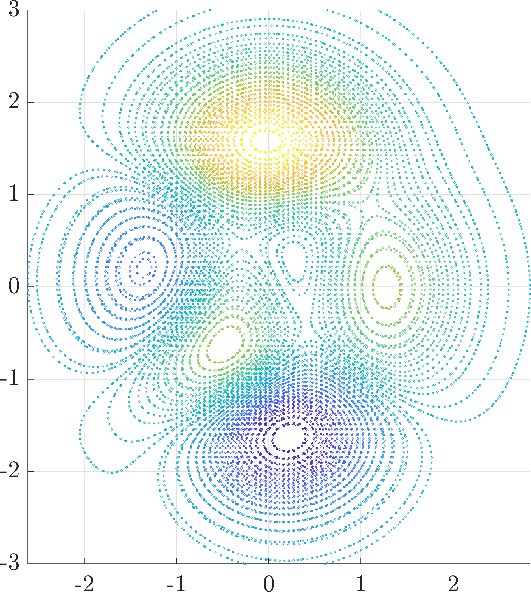
It is important to stress that the registration problem laid out here is only a local solver. However, how detrimental is this? For the purposes of gaining intuition, we will compute $F:T^{2}\to\mathbb{R}$ for the $T^{2}$ case, see Section IV-B. For the point clouds, we will use the same clouds as in Example 6 (although viewing them in $[0,2\pi)^{2}\sim T^{2}$ rather than $\mathbb{R}^{2}$). The torus is discretized into a 500 by 500 grid and length-scales are chosen in the range $[0.01,0.5]$. For each value of $\ell$, a contour plot of $F:T^{2}\to\mathbb{R}$ is constructed and the number of local maxima is recorded (with Matlab’s “imregionalmax” function). Two contour plots corresponding to $\ell=0.5$ and $\ell=0.2$ are shown in Figure 9.

It is important to note that there exists a plethora of local maxima. This illustrates how important it is to have a good initialization or else the gradient flow will end up getting trapped at a false solution.

However, the number of local solutions depends heavily on $\ell$. This can be utilized in practice by having $\ell$ start off large and shrink between iterations. It is also rather surpising that the number of local solutions seems to grow according to a power law of the length-scale, as shown in Figure 10.

XI Reduction to the Weighted Least Squares

Without loss of generality, we will use the Gaussian (Squared Exponential) kernel based on a distance function, $d(\cdot,\cdot)$:

$$k(x,y)=\sigma^{2}\exp\left(-d(x,y)^{2}\right).$$ (103)

Further, let us define $w_{ij}:=\sigma^{2}\langle\ell_{X}(x_{i}),\ell_{Z}(z_{j})\rangle_{\mathcal{I}}$ and $d_{ij}:=d(x_{i},z_{j})$. Then we have

$$\langle f_{X},f_{Z}\rangle_{\mathcal{H}}=\sum_{\begin{subarray}{c}x_{i}\in X\\ z_{j}\in Z\end{subarray}}\,w_{ij}\cdot\exp\left(-d_{ij}^{2}\right).$$ (104)

Now we explicitly apply the three assumptions that are used in the least squares problem.

Assumption 1.

The assumptions used in the least squares problem are:

1. The point clouds $X$ and $Z$ have the same number of points.

2. The point cloud $Z$ is ordered such that the matching indices are corresponding measurements.

3. The residuals are only computed between corresponding measurements.

By applying the above-mentioned assumptions to (104), we get

$$\langle f_{X},f_{Z}\rangle_{\mathcal{H}}\approx\sum_{i}\,w_{i}\cdot\exp\left(-d_{i}^{2}\right),$$ (105)

where $w_{i}=w_{ii}$ and $d_{i}=d_{ii}$. and it is reduced to a single sum over matching indices of the double sum in (104). Finally, the $\exp$ can be approximated using a Taylor expansion as

$$\exp\left(-d_{i}^{2}\right)\approx 1-d_{i}^{2}+\cdots.$$ (106)

Problem 3.

The problem of aligning the point clouds can now be rephrased as the following weighted least squares form

$$\arg\min_{h\in\mathcal{G}}\,S(h),\quad S(h):=\sum_{i}\,w_{i}\cdot d(x_{i},hz_{i})^{2}.$$ (107)

XII Conclusion

We developed a new mathematical framework for sensor registration that enables nonparametric joint semantic/appearance and geometric representation of continuous functions using data. The continuous functions allow the registration to be independent of a specific signal resolution, and the framework is fully analytical with a closed-form derivation of the Riemannian gradient and Hessian. We studied a restriction of the framework where the Lie group acts on functions isometrically. This restriction has a variety of applications, and its high-dimensional derivation for the special Euclidean group acting on the Euclidean space showcases the point cloud registration and bird’s-eye view map registration abilities. We derived low-dimensional cases with numerical examples to show the generality of the proposed framework. A specific implementation of this framework for RGB-D cameras performs well in texture and structure-scares environments and is inherently robust to the input noise.

The general problem where the Lie group does not act isometrically on the functions has interesting applications such as image registration and nonrigid structure from motion. Although, the Lie algebra of the affine matrix group does not possess any particular structure, i.e., it includes all square matrices, due to its mentioned applications it is an attractive future research direction. The development of a globally optimal solver is, of course, another challenging and attractive future research direction.

References

- [1] Y. Chen and G. Medioni, “Object modeling by registration of multiple range images,” in Proceedings of the IEEE International Conference on Robotics and Automation. IEEE, 1991, pp. 2724–2729.
- [2] A. Censi, “An ICP variant using a point-to-line metric,” in Proceedings of the IEEE International Conference on Robotics and Automation. IEEE, 2008, pp. 19–25.
- [3] A. Segal, D. Haehnel, and S. Thrun, “Generalized-ICP,” in Proceedings of the Robotics: Science and Systems Conference, vol. 2, no. 4, 2009.
- [4] T. Stoyanov, M. Magnusson, H. Andreasson, and A. J. Lilienthal, “Fast and accurate scan registration through minimization of the distance between compact 3D NDT representations,” International Journal of Robotics Research, vol. 31, no. 12, pp. 1377–1393, 2012.
- [5] J. Servos and S. L. Waslander, “Multi-Channel Generalized-ICP: A robust framework for multi-channel scan registration,” Robotics and Autonomous Systems, vol. 87, pp. 247–257, 2017.
- [6] S. A. Parkison, L. Gan, M. Ghaffari Jadidi, and R. M. Eustice, “Semantic iterative closest point through expectation-maximization,” in Proceedings of the British Machine Vision Conference, Newcastle, UK, September 2018, pp. 1–17.
- [7] A. Zaganidis, L. Sun, T. Duckett, and G. Cielniak, “Integrating deep semantic segmentation into 3-d point cloud registration,” IEEE Robotics and Automation Letters, vol. 3, no. 4, pp. 2942–2949, October 2018.
- [8] S. A. Parkison, M. Ghaffari, L. Gan, R. Zhang, A. K. Ushani, and R. M. Eustice, “Boosting shape registration algorithms via reproducing kernel Hilbert space regularizers,” IEEE Robotics and Automation Letters, vol. 4, no. 4, pp. 4563–4570, 2019.
- [9] D. Nistér, O. Naroditsky, and J. Bergen, “Visual odometry for ground vehicle applications,” Journal of Field Robotics, vol. 23, no. 1, pp. 3–20, 2006.
- [10] D. Scaramuzza and F. Fraundorfer, “Visual odometry,” IEEE robotics & automation magazine, vol. 18, no. 4, pp. 80–92, 2011.
- [11] F. Fraundorfer and D. Scaramuzza, “Visual odometry: Part ii: Matching, robustness, optimization, and applications,” IEEE Robotics & Automation Magazine, vol. 19, no. 2, pp. 78–90, 2012.
- [12] H. Strasdat, “Local accuracy and global consistency for efficient visual SLAM,” Ph.D. dissertation, Imperial College London, 2012.
- [13] C. Kerl, J. Sturm, and D. Cremers, “Dense visual slam for rgb-d cameras,” in Proceedings of the IEEE/RSJ International Conference on Intelligent Robots and Systems. IEEE, 2013, pp. 2100–2106.
- [14] J. Engel, J. Stueckler, and D. Cremers, “Large-scale direct SLAM with stereo cameras,” in Proceedings of the IEEE/RSJ International Conference on Intelligent Robots and Systems, September 2015.
- [15] M. Ghaffari, W. Clark, A. Bloch, R. M. Eustice, and J. W. Grizzle, “Continuous direct sparse visual odometry from RGB-D images,” in Proceedings of the Robotics: Science and Systems Conference, Freiburg, Germany, June 2019.
- [16] A. Rosinol, M. Abate, Y. Chang, and L. Carlone, “Kimera: an open-source library for real-time metric-semantic localization and mapping,” arXiv preprint arXiv:1910.02490, 2019.
- [17] T. Kim and Y.-J. Im, “Automatic satellite image registration by combination of matching and random sample consensus,” IEEE Transactions on Geoscience and Remote Sensing, vol. 41, no. 5, pp. 1111–1117, 2003.
- [18] Y. Bentoutou, N. Taleb, K. Kpalma, and J. Ronsin, “An automatic image registration for applications in remote sensing,” IEEE Transactions on Geoscience and Remote Sensing, vol. 43, no. 9, pp. 2127–2137, 2005.
- [19] E. M. Mikhail, J. S. Bethel, and J. C. McGlone, Introduction to modern photogrammetry. Wiley, 2001.
- [20] R. Hartley and A. Zisserman, Multiple view geometry in computer vision. Cambridge university press, 2003.
- [21] R. Szeliski, Computer vision: algorithms and applications. Springer Science & Business Media, 2010.
- [22] S. Thrun, W. Burgard, and D. Fox, Probabilistic robotics. MIT press, 2005.
- [23] T. D. Barfoot, State Estimation for Robotics. Cambridge University Press, 2017.
- [24] H. Yang and L. Carlone, “A polynomial-time solution for robust registration with extreme outlier rates,” Tech. Rep., 2019, arxiv preprint: 1903.08588.
- [25] A. Berlinet and C. Thomas-Agnan, Reproducing kernel Hilbert spaces in probability and statistics. Kluwer Academic, 2004.
- [26] B. Schölkopf, R. Herbrich, and A. Smola, “A generalized representer theorem,” in Computational learning theory. Springer, 2001, pp. 416–426.
- [27] L. Tu, Differential Geometry, ser. Graduate Texts in Mathematics. Springer, 2017.
- [28] A. Bloch, P. S. Krishnaprasad, J. E. Marsden, and T. S. Ratiu, “The Euler-Poincaré equations and double bracket dissipation,” Communications in Mathematical Physics, vol. 175, no. 1, pp. 1–42, Jan 1996.
- [29] C. M. Bishop, Pattern recognition and machine learning. Springer, 2006.
- [30] C. Rasmussen and C. Williams, Gaussian processes for machine learning. MIT press, 2006, vol. 1.
- [31] K. P. Murphy, Machine learning: a probabilistic perspective. The MIT Press, 2012.
- [32] A. M. Bloch, R. W. Brockett, and T. S. Ratiu, “Completely integrable gradient flows,” Communications in Mathematical Physics, vol. 147, no. 1, pp. 57–74, Jun 1992.
- [33] R. Berndt and M. Klucznik, An Introduction to Symplectic Geometry, ser. Graduate Studies in Mathematics. American Mathematical Society, 2001.
- [34] F. C. Park and R. W. Brockett, “Kinematic dexterity of robotic mechanisms,” International Journal of Robotics Research, vol. 13, no. 1, pp. 1–15, 1994.
- [35] V. G. Ivancevic and T. T. Ivancevic, “Lecture notes in Lie groups,” 2011.
- [36] R.-A. Rohan, “Some remarks on the exponential map on the groups SO(n) and SE(n),” in Proceedings of the Fourteenth International Conference on Geometry, Integrability and Quantization. Sofia, Bulgaria: Avangard Prima, 2013, pp. 160–175.
- [37] T.-Y. Lin, W. Clark, R. M. Eustice, J. W. Grizzle, A. Bloch, and M. Ghaffari, “Adaptive continuous visual odometry from rgb-d images,” arXiv preprint arXiv:1910.00713, 2019.
- [38] C. Kerl, J. Sturm, and D. Cremers, “Robust odometry estimation for RGB-D cameras,” in Proceedings of the IEEE International Conference on Robotics and Automation. IEEE, 2013, pp. 3748–3754.
- [39] C. Kerl, “Dense Visual Odometry (dvo),” https://github.com/tum-vision/dvo, 2013.
- [40] M. Pizenberg, “DVO core (without ROS dependency),” https://github.com/mpizenberg/dvo/tree/76f65f0c9b438675997f595471d39863901556a9, 2019.
- [41] J. Engel, T. Schöps, and D. Cremers, “LSD-SLAM: Large-scale direct monocular SLAM,” in European Conference on Computer Vision. Springer, 2014, pp. 834–849.
- [42] J. Canny, “A computational approach to edge detection,” in Readings in Computer Vision. Elsevier, 1987, pp. 184–203.
- [43] G. Bradski, “The OpenCV Library,” Dr. Dobb’s Journal of Software Tools, 2000.
- [44] Intel Corporation, “Official Threading Building Blocks (TBB) GitHub repository,” https://github.com/intel/tbb, 2019.
- [45] J. Sturm, N. Engelhard, F. Endres, W. Burgard, and D. Cremers, “A benchmark for the evaluation of rgb-d slam systems,” in Proc. of the International Conference on Intelligent Robot Systems (IROS), Oct. 2012.
- [46] J. Engel, V. Koltun, and D. Cremers, “Direct sparse odometry,” IEEE transactions on pattern analysis and machine intelligence, vol. 40, no. 3, pp. 611–625, 2018.