Many-Body Dephasing in a Trapped-Ion Quantum Simulator

Abstract

How a closed interacting quantum many-body system relaxes and dephases as a function of time is a fundamental question in thermodynamic and statistical physics. In this work, we observe and analyse the persistent temporal fluctuations after a quantum quench of a tunable long-range interacting transverse-field Ising Hamiltonian realized with a trapped-ion quantum simulator. We measure the temporal fluctuations in the average magnetization of a finite-size system of spin-$1/2$ particles and observe the experimental evidence for the theoretically predicted regime of many-body dephasing. We experiment in a regime where the properties of the system are closely related to the integrable Hamiltonian with global spin-spin coupling, which enables analytical predictions even for the long-time non-integrable dynamics. We find that the measured fluctuations are exponentially suppressed with increasing system size, consistent with theoretical predictions.

Introduction.– Investigating the relaxation and dephasing dynamics of a closed many-body quantum system is of paramount importance to the study of thermodynamics and statistical physics. Most commonly, this problem is investigated by studying the time evolution of the expectation value of a local observable, e.g., particle density or magnetization, after quenching the system from an initial out-of-equilibrium state [1, 2]. For a generic nonintegrable system, the expectation value tends to relax to a constant in the thermodynamic limit which can be described by a thermal state at some temperature depending on the initial state [3, 4, 5, 1, 2, 8, 9]. However, if the system size is finite, there exist persistent temporal fluctuations around the constant average value, as sketched in Fig. 1(a). Importantly, these persistent temporal fluctuations in the expectation value after a quench are distinct from the usual fluctuations of observables in equilibrium (where expectation values are constant). Studying these temporal fluctuations represents the next level of the description of quench dynamics going beyond merely looking at long-time observable averages.

A crucial question for statistical physics is how the temporal fluctuations are suppressed with increasing system size $N$. In the case of integrable systems mappable to free quasiparticles, it has been found that the variance of temporal fluctuations scales as $1/N$ [10, 11, 12]. In the case of generic nonintergrable systems [13, 14, 15, 16, 17, 18], or the integrable systems solvable with the Bethe ansatz (not mappable to noninteracting ones) [19], the temporal fluctuations are exponentially suppressed by the system size due to the highly nondegenerate spectrum. This was first found only numerically. However, in Ref. [18], the authors were able, for the first time, to provide an exact analytical result for the exponential scaling of fluctuations with $N$ spins in a weakly nonintegrable system. In this setting, they identified a general dynamical regime which they termed “many-body dephasing”[20]. In the thermalization process, the dephasing mechanism comes from the relaxation of the quasiparticle distribution to thermal equilibrium by quasiparticle scattering described by the Boltzmann equation. In contrast, many-body dephasing results from lifting of the exponentially large degeneracies of transition energies in integrable systems while the quasiparticle distribution remains practically unchanged [18].

Nevertheless, the exponential size scaling due to many-body dephasing in nonintegrable systems has not yet been verified in experiments. Here, we give the first experimental observation of persistent temporal fluctuations after a quantum quench characterized as a function of system size, employing a trapped-ion quantum simulator. We present a direct measurement of relaxation dynamics in the nonintegrable system by measuring the temporal fluctuations in the average magnetization of a finite-size system of spin-$1/2$ particles. After including the experimental noise in the data analysis, the temporal fluctuations from experimental data are consistent with our numerical simulations and theoretical analysis based on the concept of many-body dephasing.

Figure 1: (a) Schematic behaviour of an observable $\langle A(t)\rangle$ after a quench, in a finite-size system. (b) Temporal fluctuation $\sigma_{A}$ for $N=7$ spins (left) and size scaling exponent $\kappa$ (right) as a function of power-law coupling exponent $\alpha$ for three fixed parameters $\lambda=2J_{0}/B$. The vertical dashed lines indicate the crossover values of $\alpha^{*}=\ln(2|\lambda|)/\ln 2$ [24].

Model Hamiltonian.– The Hamiltonian implemented in this experiment is the long-range transverse-field Ising model,

$$H=\sum_{i<j}J_{ij}\sigma_{i}^{x}\sigma_{j}^{x}-\frac{1}{2}B\sum_{i}\sigma_{i}^{z},$$ (1)

where $J_{ij}\approx J_{0}/|i-j|^{\alpha}>0$, is a long-range coupling that falls off approximately as a tunable power-law. The Hamiltonian (1) is implemented using an applied laser field which creates spin-spin interactions through spin-dependent optical dipole forces. The spin chain is initialized to the $|\!\!\downarrow\downarrow...\downarrow\rangle_{z}$ state, then a quench is performed using Hamiltonian (1), and the magnetization along the $\hat{z}$ axis is measured as a function of time. The cases of $\alpha^{-1}=0$ and $\alpha=0$ correspond to two integrable limits, i.e., the nearest neighbour coupling and global coupling models respectively. For a finite $\alpha>0$, Hamiltonian (1) is in general nonintegrable.

Temporal fluctuations.– In the present experiment, the observable is the magnetization, i.e., $A=N^{-1}\sum_{j}{\sigma_{j}^{z}}$. The temporal average of the variable $\langle A(t)\rangle$ is calculated as $\overline{\langle A(t)\rangle}\equiv T^{-1}\int_{t_{i}}^{t_{i}+T}\langle A(t)\rangle dt$, where the temporal averaging is restricted within the time window between $t_{i}$ and $t_{i}+T$. The variance of temporal fluctuations of $\langle A(t)\rangle$ is defined via $\sigma_{A}^{2}\equiv\overline{\big(\langle A(t)\rangle-\overline{\langle A(t)\rangle}\big)^{2}}$, with $\sigma_{A}$ the standard deviation. We use $|\Phi_{n}\rangle$ ($n=1,2,\cdots,2^{N}$) to represent the many-body eigenstates of Hamiltonian (1) with eigenenergy $E_{n}$. Given the initial state $|\psi(0)\rangle$, the exact time evolution of the observable is $\langle A(t)\rangle=\sum_{m,n}\langle\psi(0)|\Phi_{m}\rangle\langle\Phi_{m}|A|\Phi_{n}\rangle\langle\Phi_{n}|\psi(0)\rangle e^{i\Delta_{mn}t},$ where $\Delta_{mn}\equiv E_{m}-E_{n}$ is the transition energy between the two energy levels $|\Phi_{m}\rangle$ and $|\Phi_{n}\rangle$ ($\hbar=1$). It is not difficult to prove that, in the long time window limit ($T\rightarrow+\infty$), we have the temporal average

$$\overline{\langle A(t)\rangle}=\sum_{m,n,\Delta_{mn}=0}\langle\psi(0)|\Phi_{m}\rangle\langle\Phi_{m}|A|\Phi_{n}\rangle\langle\Phi_{n}|\psi(0)\rangle$$

and the variance of temporal fluctuation

$$\sigma^{2}_{A}=\sum_{\Delta\neq 0}\Big|\sum_{\Delta_{mn}=\Delta}\langle\psi(0)|\Phi_{m}\rangle\langle\Phi_{m}|A|\Phi_{n}\rangle\langle\Phi_{n}|\psi(0)\rangle\Big|^{2}$$ (2)

with $\Delta$ denoting the set of all the possible values of $\Delta_{mn}$. For the integrable models ($\alpha^{-1}=0$ and $\alpha=0$), there are exponentially many degeneracies with the number of spins for a given transition energy $\Delta_{mn}$, since each many-body eigenstate can be labelled by many independent conserved quantities. However, for a generic nonintegrable model with finite $\alpha>0$, there are no conserved quantities except the Hamiltonian itself. Thus, it is reasonable to assume that all the degeneracies of transition energies are lifted, making $\Delta_{mn}=0$ only possible for $m=n$ in the nonintegrable model, so Eq. (2) simplifies to

$$\sigma^{2}_{A} = \sum_{m\neq n}\Big|\langle\psi(0)|\Phi_{m}\rangle\langle\Phi_{m}|A|\Phi_{n}\rangle\langle\Phi_{n}|\psi(0)\rangle\Big|^{2}.$$ (3)

Upon closer analysis, this is the basic reasoning that leads to the exponential suppression of fluctuations with system size [13]. However, in general cases, it is impossible to evaluate this expression analytically.

Theoretical results.– We investigated numerically the temporal fluctuation $\sigma_{A}$ as a function of $\alpha$ for fixed dimensionless parameter $\lambda\equiv 2J_{0}/B$. We also extract from our numerical simulations the size scaling exponent $\kappa$ from the fit $\sigma_{A}\propto e^{-\kappa N}$ by calculating $\sigma_{A}$ for $N=3-10$ spins (see Fig. 1(b)). We find two distinct regimes, at small and large $\alpha$, separated by the crossover value of $\alpha^{*}=\ln(2|\lambda|)/\ln 2$ [24]. The crossover between those regimes can be understood from the competition between the two terms in Hamiltonian (1), i.e., the magnetic field energy $-B\sum_{i}s^{z}_{i}$ (where $s^{z}_{i}\equiv\frac{1}{2}\sigma_{i}^{z}$ is the spin operator) and the next-nearest-neighbor (NNN) spin-spin coupling $2^{-\alpha}4J_{0}\sum_{i}s_{i}^{x}s_{i+2}^{x}$, which, for $\alpha>0$, is the leading term responsible for breaking integrability [24]. In the regime of $\alpha\gg\alpha^{*}$, by neglecting the NNN coupling (and other long-range coupling terms), the Hamiltonian is reduced into an integrable model with NN coupling. Adding the NNN coupling terms weakly breaks the integrability and results in many-body dephasing [18]. We cannot reach this regime in the experiment since the power-law exponent is $\alpha\approx 0.7$. Therefore this work lies in the opposite regime of $\alpha\ll\alpha^{*}$, where the long-range coupling terms are dominant over the magnetic field energy. The general concept of many-body dephasing still applies in this regime, and an analytical prediction can be obtained, as we will show below.

We start our analysis from the global coupling limit $\alpha=0$:

$$H_{\alpha=0}=-B{S}^{z}_{N}+2J_{0}(S^{x}_{N})^{2}+NJ_{0}/2.$$ (4)

The Hamiltonian (4) is also called Lipkin-Meshkov-Glick (LMG) model [32], which is integrable [33, 34] since there exist $N$ conserved quantities. For example, $\vec{S}^{2}_{n}\equiv S^{x2}_{n}+S^{y2}_{n}+S^{z2}_{n}$ ($n=2,\dots,N$) and the Hamiltonian (4) itself satisfy $[\vec{S}^{2}_{n},H_{\alpha=0}]=0$, where $S^{\beta}_{n}\equiv\sum^{n}_{i=1}\frac{1}{2}\sigma^{\beta}_{i}$ with $\beta=x,y,z$. In the special case of $\lambda\rightarrow\infty$ ($B\rightarrow 0$), we can label each energy level by $|S_{1},S_{2},\cdots,S_{N-1},S_{N},S^{x}_{N}\rangle$ and group all the eigenstates into $N+1$ subspaces according to $S^{x}_{N}$. In each subspace of $S^{x}_{N}$, we can prove that there are ${N\choose N/2+S^{x}_{N}}$ degenerate levels. For finite $\alpha>0$, since the interaction term in Hamiltonian (1) keeps the total spin projection $S^{x}_{N}$ unchanged, the eigenstates in different $S^{x}_{N}$-subspaces are decoupled. All the degenerate eigenstates in the same $S^{x}_{N}$-subspace couple each other resonantly and form new hybridized eigenstates $|\Phi_{n}\rangle$ appearing in Eq. (2). To estimate $\sigma_{A}$ in Eq. (3), we assume each many-body eigenstate $|\Phi_{n}\rangle$ to be a superposition of all the ${N\choose N/2+S^{x}_{N}}$ levels in the $S^{x}_{N}$-subspace with probabilities fluctuating about their uniformly distributed value ${N\choose N/2+S^{x}_{N}}^{-1}$.

We define the notation $|\Phi^{\lambda=\infty}_{\frac{N}{2},S^{x}_{N}}\rangle$ as the eigenstate of Hamiltonian (4) with $S_{N}=N/2$ and spin projection $S^{x}_{N}$ at $\lambda=\infty$. In the experiment, the pre-quenched spin state is $|\psi(0)\rangle=|\!\downarrow,\downarrow,\cdots,\downarrow\rangle_{z}$ which only couples the states with total spin $S_{N}=N/2$. Since $|\Phi^{\lambda=\infty}_{\frac{N}{2},S^{x}_{N}}\rangle$ is the only component with total spin $S_{N}=N/2$ of the many-body $|\Phi_{n}\rangle$ in the $S^{x}_{N}-$subspace, we have

$$\big|\langle\psi(0)|\Phi_{n}\rangle\big|^{2}\approx{N\choose N/2+S^{x}_{N}}^{-1}P^{\lambda=\infty}_{\frac{N}{2},S^{x}_{N}},$$ (5)

where $P^{\lambda=\infty}_{\frac{N}{2},S^{x}_{N}}\equiv\big|\langle\psi(0)|\Phi^{\lambda=\infty}_{\frac{N}{2},S^{x}_{N}}\rangle\big|^{2}$ is the probability of initial state $|\psi(0)\rangle$ being $|\Phi^{\lambda=\infty}_{\frac{N}{2},S^{x}_{N}}\rangle$. Based on this assumption and the eigenstate thermalization hypothesis (ETH) [1, 2, 3, 4, 5], we are able to obtain an approximate formula for Eq. (3)

$$\sigma^{2}_{A}\approx 2\sum_{S^{x}_{N},S^{\prime x}_{N}}\frac{P^{\lambda=\infty}_{\frac{N}{2},S^{x}_{N}}P^{\lambda=\infty}_{\frac{N}{2},S^{\prime x}_{N}}}{{N\choose N/2+S^{x}_{N}}+{N\choose N/2+S^{\prime x}_{N}}}\Big|A^{\lambda=\infty}_{S^{x}_{N}S^{\prime x}_{N}}\Big|^{2}$$ (6)

with the matrix element $A^{\lambda=\infty}_{S^{x}_{N}S^{\prime x}_{N}}\equiv\langle\Phi^{\lambda=\infty}_{\frac{N}{2},S^{x}_{N}}|A|\Phi^{\lambda=\infty}_{\frac{N}{2},S^{\prime x}_{N}}\rangle$. For large $N$, we have the asymptotic expression that ${N\choose N/2+S^{x}_{N}}\sim 2^{N}\sqrt{\frac{2}{N\pi}}e^{-2(S^{x}_{N})^{2}/N}.$ The denominator of Eq. (6) indicates that $\sigma_{A}\propto 2^{-N/2}=e^{-N\ln\sqrt{2}}$, predicting the size scaling exponent $\kappa=\ln\sqrt{2}\approx 0.35$. Considering both $\lambda$ and $\alpha$ finite, the formula (6) holds as long as $\alpha\ll\alpha^{*}$. However, the eigenstate $|\Phi^{\lambda}_{\frac{N}{2},S^{x}_{N}}\rangle$ refers to the eigenlevel adiabatically connected to $|\Phi^{\lambda=\infty}_{\frac{N}{2},S^{x}_{N}}\rangle$. In general, there is no simple closed form for the eigenstate $|\Phi^{\lambda}_{\frac{N}{2},S^{x}_{N}}\rangle$ with a finite $\lambda$ [35]. However, Eq. (6) reduces the calculation of $\sigma_{A}$ to an $N\times N$ eigenvalue problem which can easily be solved on a computer. As we will show further below, the analytical predictions compare well with the experiment (see Fig. 4(a)).

Figure 2: Time evolution of average magnetization, $\langle A\rangle=N^{-1}\sum_{j}\langle\sigma_{j}^{z}\rangle$, over $N=4$ ions out to $2\text{\,}\mathrm{ms}$ for $B=+2\pi\times$0.5\text{\,}\mathrm{kHz}$$ (a) and $B=-2\pi\times$0.5\text{\,}\mathrm{kHz}$$ (b). Each data point is the average of $4000$ experiments. For both plots: Blue are data points, Black and Red are theoretical results with $(\sigma_{J_{0}},\sigma_{B})=0$ and $(\sigma_{J_{0}},\sigma_{B})=2\pi\times(0.1,0.1)$\mathrm{kHz}$$ respectively.

Figure 3: Temporal fluctuation $\sigma_{A}$ as a function of $\lambda=2J_{0}/B$ for $N=3-8$ ions from experimental data (blue dots with error bars) and from numerical simulations (blue curves) with parameters: $(\sigma_{J_{0}},\sigma_{B})=2\pi\times(0.12,0.12)\,$\mathrm{kHz}$$ for $N=3$, $2\pi\times(0.10,0.10)\,$\mathrm{kHz}$$ for $N=4$, $2\pi\times(0.11,0.11)\,$\mathrm{kHz}$$ for $N=5$ and $2\pi\times(0.09,0.09)\,$\mathrm{kHz}$$ for $N=6-8$.

Experimental results.– To perform this experiment, each effective spin $1/2$ particle is encoded in the hyperfine ground state of one ¹⁷¹Yb⁺ with $|\!\!\uparrow\rangle\equiv^{2}$S${}_{1/2}|F=1,m_{F}=0\rangle$ and $|\!\!\downarrow\rangle\equiv^{2}$S${}_{1/2}|F=0,m_{F}=0\rangle$. The Hamiltonian of Eq. (1) is realized by global spin-dependent optical dipole forces from laser beams, which modulate the Coulomb interaction to create an effective Ising coupling between spins [36]. The field term is implemented by asymmetrically detuning the two laser beatnotes generating the optical dipole forces.

The magnetization fluctuations $\sigma_{A}$ are characterized by measuring the standard deviation of the average magnetization of the sum of all ions in the chain, i.e., $\langle A\rangle=N^{-1}\sum_{j}\langle\sigma_{j}^{z}\rangle$. This is measured with B-fields ranging from $\pm$ $2\pi\times$0.5\text{\,}\mathrm{kHz}$$ to $2\pi\times$2.0\text{\,}\mathrm{kHz}$$. The two plots in Fig. 2 show the magnetization data measured as a function of time with a $4$-ion chain and $B=\pm 2\pi\times$0.5\text{\,}\mathrm{kHz}$$. Although the decoherence time in our trapped-ion simulator is long enough to consider $J_{0}$ and $B$ unchanged within a single time evolution up to $t=2\,$\mathrm{ms}$$, the values of $J_{0}$ and $B$ may vary between different time evolutions. We assume the coupling strength and magnetic field in the experiments to be independent and normally distributed. Then, the averaged observable $A$ at a fixed time $t$ also needs to be averaged over the experimental values of $J_{0}$ and $B$, resulting in:

$$\langle A(t)\rangle=\langle\langle\psi(t)|A|\psi(t)\rangle\rangle_{J_{0},B}.$$ (7)

In Fig. 2, the red curves are the theory fits by setting $\sigma_{J_{0}}$ and $\sigma_{B}$ both to approximately $2\pi\times$0.1\text{\,}\mathrm{kHz}$$. To fit the experimental data, we use the gradient descent method to search for the optimal values of $\sigma_{J_{0}}$ and $\sigma_{B}$, which happen to be roughly equal. Therefore, we set $\sigma_{J_{0}}$ and $\sigma_{B}$ to be the same values for simplicity.

In general, with a positive B-field, we observe more significant oscillations than when using a negative B-field. This can be understood by analyzing the overlap between the pre-quench state and the post-quench energy eigenstates (obtained for the post-quench $J_{0}$ and $B$ values). For the system parameters given in Fig. 2, the structure of the post-quench spectrum is such that at high energies there is a non-vanishing energy gap in the thermodynamic limit. Conversely, in the low energy sector of the spectrum the level spacing decreases with system size and the gap vanishes in the thermodynamic limit. For the positive B-field, the pre-quench state is the superposition of several of the highest excited states of the spectrum and the energy gap leads to more persistent oscillations. For the negative B-field, the pre-quench state is very close to the ground state of the spectrum [37], suppressing the oscillations.

We plot the standard deviation of the average magnetization $\sigma_{A}$ as a function of $\lambda=2J_{0}/B$ for fixed $N$ in Fig. 3. The data for $N=3$ to $N=6$ agree with the theoretical prediction. The $N=7$ data largely agrees with theory excluding the two outlying points at negative $\lambda$ values. For $N=8$, the data points tend to gather around the 0.07 level indicating that the measurement noise in this case obscures the measured fluctuations. In these plots, the values near $\lambda=0$ were not taken because when $B\gg J_{0}$ the ions are predominantly acting paramagnetically. In this regime, fluctuations are expected to be very small and well below the noise floor of this experiment. The shape of the data is asymmetric with a pronounced slope at $2J_{0}/B=1/2$. This point marks the ferromagnetic (FM) to paramagnetic (PM) phase transition of the ion chain. The fluctuations are enhanced here as this is an unstable point for the system. In contrast, the antiferromagnetic (AFM) to PM transition [38] for $\lambda<0$ is not as pronounced.

Figure 4: Logplot of temporal fluctuation $\sigma_{A}$ versus number of spins $N$: (a) Numerical results with different time windows and analytical results from Eq. (6). Here $\alpha=0.7$ and $\lambda=1.7$. (b) Experimental results at $\lambda\approx 1.7$ versus numerical results with $(J_{0},B)=2\pi\times(0.5,0.59)\,$\mathrm{kHz}$$, $(\sigma_{J_{0}},\sigma_{B})=2\pi\times(0.1,0.1)\,$\mathrm{kHz}$$ and $\alpha=0.7$. Dashed lines are the fits.

System size scaling.– The temporal fluctuation variance $\sigma^{2}_{A}$ given by Eq. (3) is obtained by averaging over an infinite time window $J_{0}t\in[0,+\infty]$. However, in the experiment, we can only average over a finite time window up to $t\sim 2.0\,$\mathrm{ms}$$ ( i.e., 3 or 4 oscillations depending on the value of $\lambda$), as the long-time fluctuations are suppressed by the noise in the Hamiltonian parameters $J_{0}$ and $B$. Fig. 4(a) shows that short-time-window averaging only makes sense for small system size, e.g., the time window $J_{0}t\in[0,2\pi]$ works up to $N=6$ spins. Larger system sizes result in smaller level splittings and makes the period of temporal fluctuations longer, thus necessitating a longer time window to calculate the temporal fluctuations. We compare the numerical results from Eq. (3) (red empty circles) and with the analytical result from Eq. (6) (solid blue dots), showing good agreement. The fit to the infinite-time-window averaging (red dashed line) shows that the system size scaling exponent is $\kappa\approx 0.35$ consistent with the theoretical prediction $\kappa=\ln\sqrt{2}$. In Fig. 4(b), we compare the experimental data (black dots with error bars) with the numerical results (red circle dots) by averaging over the finite time window $t\in[0.08\,$\mathrm{ms}$,2.0\,$\mathrm{ms}$]$. The finite variances $\sigma_{J_{0}}$ and $\sigma_{B}$ reduce the temporal fluctuations and also set a lower limit for the measurement accuracy, as indicated by the blue region in the figure. As a result, only the first three data points ($N=3-5$) provide the information on system size scaling. The fits to the experimental and numerical values of $\sigma_{A}$ for $N=3-5$ (dashed lines) both show a clear exponential size suppression with the scaling exponent $\kappa\approx 0.24$, smaller than the ideal scaling exponent $\kappa\approx 0.35$ shown in Fig. 4(a). This is caused by the experimental drifts in the Hamiltonian parameters $J_{0}$ and $B$. Indeed with larger $\sigma_{J_{0}}$ and $\sigma_{B}$, the measured fluctuations $\sigma_{A}$ versus number of spins $N$ would be completely flat as shown in the interval $N=6-8$ in Fig.  4(b) and the extracted scaling exponent $\kappa$ would be zero.

Summary.– Using our trapped-ion quantum simulator, we present the first experimental observation of persistent temporal fluctuations after a quantum quench with a long-range interacting transverse-field Ising model. We characterized how the fluctuations in the average magnetization of the spin chain depend on the transverse field and the spin-spin interactions. This experiment was performed in the near-integrable regime where analytical solutions are available, though the system is non-integrable. Numerical simulations compared with experiment show that, as a function of system size $N$, the exponential suppression of temporal fluctuations matches well with the theoretical value.

I Supplemental Material to
Many-Body Dephasing in a Trapped Ion Quantum Simulator

I.1 I. Temporal fluctuations

Here, our aim is to calculate the variance of temporal fluctuation given by

$$\sigma^{2}_{A} = \sum_{m\neq n}\Big|\langle\psi(0)|\Phi_{m}\rangle\langle\Phi_{m}|A|\Phi_{n}\rangle\langle\Phi_{n}|\psi(0)\rangle\Big|^{2}.$$ (8)

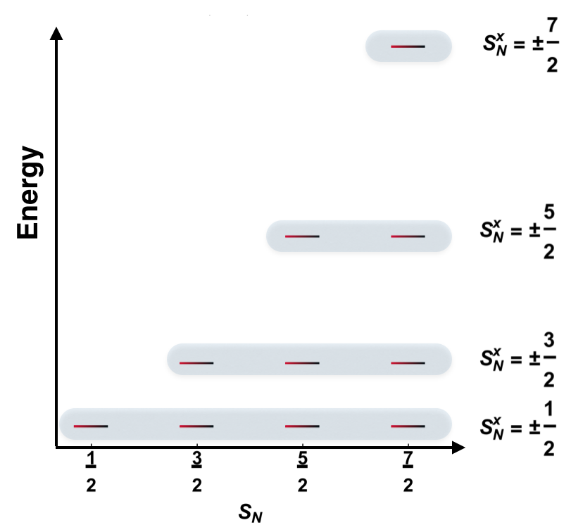
We use $|\Phi^{S^{x}_{N}}_{n}\rangle$ to represent the eigenstate in the $S^{x}_{N}$-subspace (see the energy level structure in Fig. 5). The above expression can be written alternatively

$$\sigma^{2}_{A} = \sum_{S^{x}_{N},S^{\prime x}_{N}}\sum_{m\neq n}\Big|\langle\psi(0)|\Phi^{S^{x}_{N}}_{m}\rangle\langle\Phi^{S^{x}_{N}}_{m}|A|\Phi^{S^{\prime x}_{N}}_{n}\rangle\langle\Phi^{S^{\prime x}_{N}}_{n}|\psi(0)\rangle\Big|^{2}.$$ (9)

Using Eq. (5) in the main text, we have

$$\sigma^{2}_{A} \approx \sum_{S^{x}_{N},S^{\prime x}_{N}}P^{\lambda=\infty}_{\frac{N}{2},S^{x}_{N}}P^{\lambda=\infty}_{\frac{N}{2},S^{\prime x}_{N}}\sum_{m\neq n}\frac{\Big|\langle\Phi^{S^{x}_{N}}_{m}|A|\Phi^{S^{\prime x}_{N}}_{n}\rangle\Big|^{2}}{{N\choose N/2+S^{x}_{N}}{N\choose N/2+S^{\prime x}_{N}}}\$$ (10)

with $P^{\lambda=\infty}_{\frac{N}{2},S^{x}_{N}}\equiv\big|\langle\psi(0)|\Phi^{\lambda=\infty}_{\frac{N}{2},S^{x}_{N}}\rangle\big|^{2}$. By further defining

$$\overline{A^{2}}_{S^{x}_{N},S^{\prime x}_{N}} \equiv \sum_{m\neq n}\frac{\Big|\langle\Phi^{S^{x}_{N}}_{m}|A|\Phi^{S^{\prime x}_{N}}_{n}\rangle\Big|^{2}}{{N\choose N/2+S^{x}_{N}}{N\choose N/2+S^{\prime x}_{N}}}=\sum_{m,n}\frac{\Big|\langle\Phi^{S^{x}_{N}}_{m}|A|\Phi^{S^{\prime x}_{N}}_{n}\rangle-\langle\Phi^{S^{x}_{N}}_{m}|A|\Phi^{S^{\prime x}_{N}}_{n}\rangle\delta_{mn}\Big|^{2}}{{N\choose N/2+S^{x}_{N}}{N\choose N/2+S^{\prime x}_{N}}},\ \ \ \$$ (11)

we obtain the compact form

$$\sigma^{2}_{A} \approx \sum_{S^{x}_{N},S^{\prime x}_{N}}P^{\lambda=\infty}_{\frac{N}{2},S^{x}_{N}}P^{\lambda=\infty}_{\frac{N}{2},S^{\prime x}_{N}}\overline{A^{2}}_{S^{x}_{N},S^{\prime x}_{N}}.$$ (12)

According to the eigenstate thermalization hypothesis (ETH)[1, 2, 3, 4, 5], we have

$$\langle\Phi^{S^{x}_{N}}_{m}|A|\Phi^{S^{\prime x}_{N}}_{n}\rangle\approx\overline{A}\delta_{mn}+\sqrt{\frac{\overline{A^{2}}}{D}}R_{mn}$$ (13)

where $\overline{A}$ and $\overline{A^{2}}$ are smooth functions of energy levels, $R_{mn}$ is a random variable with zero mean and unit variance, $D$ is the many-body Hilbert space dimension. Since the observable we consider here $A=N^{-1}\sum_{j}\sigma^{z}_{j}=2N^{-1}S^{z}_{N}$ only couples the neighboring $S^{x}_{N}$-subspaces, i.e., $S^{\prime x}_{N}=S^{x}_{N}\pm 1$, we thus set $D={N\choose N/2+S^{x}_{N}}+{N\choose N/2+S^{\prime x}_{N}}$.

Figure 5: Energy level structure of $N=7$ ions in the global coupling limit ($\alpha=0$) for the parameter $\lambda\rightarrow\infty$ ($i.e.,B\rightarrow 0$). $S_{N}$ is the spin quantum number of $N$ ions and $S^{x}_{N}$ is the total spin component along the $x$-axis. Each row contains two $S^{x}_{N}$-subspaces with opposite sign $S^{x}_{N}$. Finite-$\alpha$ coupling term in the Hamiltonian hybridizes the levels inside each $S^{x}_{N}$-subspace while finite-$B$ term couples the levels in the neighboring $S^{x}_{N}$-subspaces.

We see that the quantity $\overline{A^{2}}_{S^{x}_{N},S^{\prime x}_{N}}$ given by Eq. (11) is just the variance of the random part in the matrix element Eq. (13), which can be calculated

$$\overline{A^{2}}_{S^{x}_{N},S^{\prime x}_{N}}=\frac{\overline{A^{2}}}{{N\choose N/2+S^{x}_{N}}+{N\choose N/2+S^{\prime x}_{N}}}.$$ (14)

Therefore, we have the variance of temporal fluctuations from Eq. (12)

$$\sigma^{2}_{A} \approx \sum_{S^{x}_{N},S^{\prime x}_{N}}\frac{P^{\lambda=\infty}_{\frac{N}{2},S^{x}_{N}}P^{\lambda=\infty}_{\frac{N}{2},S^{\prime x}_{N}}}{{N\choose N/2+S^{x}_{N}}+{N\choose N/2+S^{\prime x}_{N}}}\overline{A^{2}}.$$ (15)

To estimate the pre-factor $\overline{A^{2}}$ in the above expression, we calculate $\sigma^{2}_{A}$ in the global coupling limit of $\alpha=0$. In this case, since the total spin quantum number of the initial state (all the spins down along $z$-direction) is $S_{N}=N/2$, we only need to consider the $S_{N}$-subspace. Therefore, we have the temporal fluctuation directly from Eq. (9)

$$\sigma^{2}_{A} = \sum_{S^{x}_{N},S^{\prime x}_{N}}{P^{\lambda=\infty}_{\frac{N}{2},S^{x}_{N}}P^{\lambda=\infty}_{\frac{N}{2},S^{\prime x}_{N}}}\Big|\langle\Phi^{\lambda=\infty}_{\frac{N}{2},S^{x}_{N}}|A|\Phi^{\lambda=\infty}_{\frac{N}{2},S^{\prime x}_{N}}\rangle\Big|^{2}.$$ (16)

The above expression (16) can be considered as the special case of the expression (15). Because there is only one level in each $S^{x}_{N}$-subsapce, the Hilbert space dimension is $D=2$. Therefore, we identify the pre-factor

$$\overline{A^{2}}=2\Big|\langle\Phi^{\lambda=\infty}_{\frac{N}{2},S^{x}_{N}}|A|\Phi^{\lambda=\infty}_{\frac{N}{2},S^{\prime x}_{N}}\rangle\Big|^{2}.$$

Finally, we obtain the formula (6) in the main text, i.e.,

$$\sigma^{2}_{A}\approx 2\sum_{S^{x}_{N},S^{\prime x}_{N}}\frac{P^{\lambda=\infty}_{\frac{N}{2},S^{x}_{N}}P^{\lambda=\infty}_{\frac{N}{2},S^{\prime x}_{N}}\Big|A^{\lambda=\infty}_{S^{x}_{N}S^{\prime x}_{N}}\Big|^{2}}{{N\choose N/2+S^{x}_{N}}+{N\choose N/2+S^{\prime x}_{N}}}$$ (17)

with the matrix element defined by

$$A^{\lambda=\infty}_{S^{x}_{N}S^{\prime x}_{N}}\equiv\langle\Phi^{\lambda=\infty}_{\frac{N}{2},S^{x}_{N}}|A|\Phi^{\lambda=\infty}_{\frac{N}{2},S^{\prime x}_{N}}\rangle.$$

As we mentioned in the main text, we expect the formula (17) still works for a finite value of $\lambda$, by referring the eigenstate $|\Phi^{\lambda}_{\frac{N}{2},S^{x}_{N}}\rangle$ to the eigenlevel adiabatically connecting to $|\Phi^{\lambda=\infty}_{\frac{N}{2},S^{x}_{N}}\rangle$.

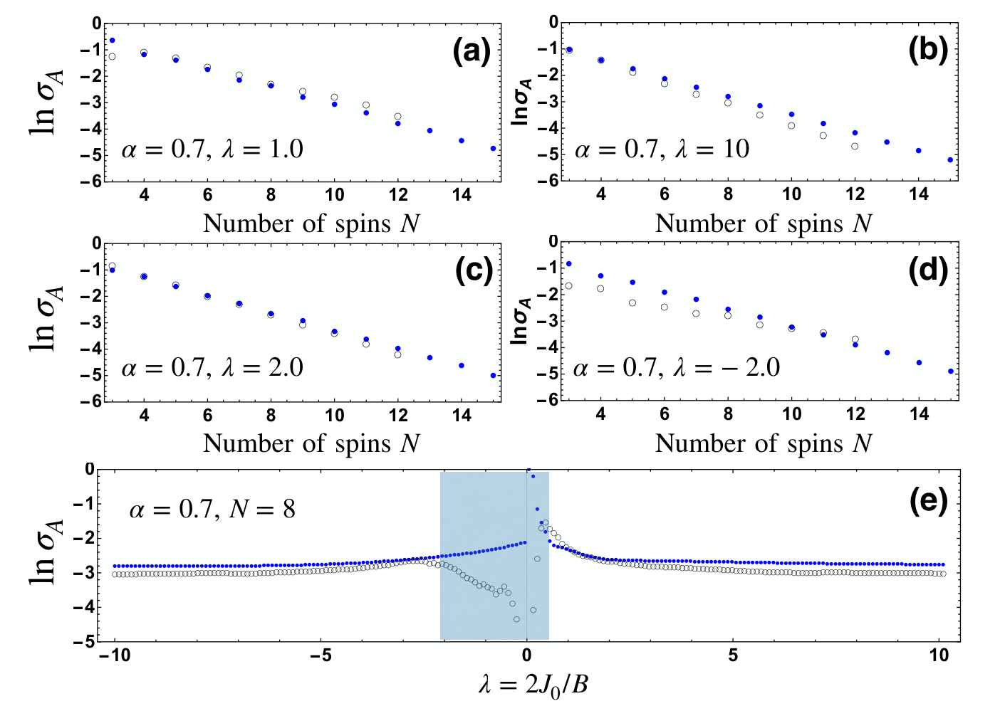
We emphasize that several physical assumptions are made in the derivation of Eq. (17). The validity of Eq. (17) is verified numerically as shown by Fig. 6. In Figs. (a)-(d), we compare the temporal fluctuations $\ln\sigma_{A}$ as function of $N$ calculated from exact diagonalization (black empty circles) and analytical formula (17) (blue solid dots) for different parameter settings. They agree with each other very well. As discussed in the main text, Eq. (17) is valid in the parameter regime $\alpha\ll\alpha^{*}=\ln(2|\lambda|)/\ln 2.$ Thus, for a fixed $\alpha>0$, it needs that $|\lambda|\gg 2^{\alpha-1}$. In Fig. 6(e), we show that Eq. (17) fails when the parameter $\lambda$ is in the regime $-2.0\lesssim\lambda\lesssim 0.5$ for $\alpha=0.7$ as indicated by the dark region. For the parameter $|\lambda|\leq 0.5$, the critical value of power-law exponent $\alpha^{*}\leq 0$; thus no value of $\alpha>0$ satisfies Eq. (17).

Figure 6: Compare the temporal fluctuations $\ln\sigma_{A}$ calculated from exact diagonalization up to $N=12$ spins (black empty circles) and analytical formula Eq. (17) up to $N=15$ spins (blue solid dots). Figs. (a-d) show $\ln\sigma_{A}$ as functions of system size $N$ while Fig. (e) shows $\ln\sigma_{A}$ as a function of $\lambda$.

I.2 II. Trapped-Ion experimental system

The ions are trapped in a macroscopic linear Paul trap with transverse center-of-mass (COM) trap frequency $\nu_{COM}=4.4$ MHz. The trap is housed in a cryogenic vacuum chamber in order to reduce the background vacuum pressure [6]. To conduct the experiment, the spins are initialized into the $|\!\downarrow\downarrow...\downarrow\rangle_{z}$ state by optical pumping with resonant 369.5 nm light. Coherent spin rotations and spin-spin interactions are performed using 355 nm counter-propagating Raman beams.

In order to generate the Hamiltonian (1) in the main text, we use the Mølmer-Sørensen (MS) protocol [7] by applying a bichromatic Raman beatnote at frequencies $\omega_{0}\pm\mu$, where $\omega_{0}/2\pi=12.643$ GHz is the qubit frequency. The bichromatic beat-notes off-resonantly excite the transverse modes of motion generating the Ising Hamiltonian [8].

$$H=\sum_{i<j}J_{ij}\sigma^{x}_{i}\sigma^{x}_{j},\,\,\,J_{ij}=\Omega^{2}\omega_{R}\sum_{m}\frac{b_{im}b_{jm}}{\mu^{2}-\omega_{m}^{2}}.$$ (18)

Here $\Omega$ is the global carrier Rabi frequency coupling the electronic states $\ket{\downarrow}_{z}$ and $\ket{\uparrow}_{z}$, $\omega_{R}=\hbar\Delta k^{2}/(2M)$ is the recoil frequency, $b_{im}$ is the normal mode transformation matrix of the $i$-th ion with the $m$th normal mode, $\Delta k$ is the difference wave-vector between the two Raman beat-notes, $M$ is the mass of a single ion, and $\omega_{m}$ is the frequency of the $m$-th normal mode. Equation (18) shows that the collective modes of vibration of the ion chain mediate the long-range spin-spin coupling. The transverse field, along $\hat{z}$, is created by providing an asymmetric frequency shift $\pm\mu\rightarrow\pm\mu+B$ to the red and blue Raman beat-notes, generating an effective magnetic field $B/2$ [9].

Following an experiment, we measure each spin’s magnetization with spin-dependent fluorescence using Andor iXon Ultra 897 EMCCD camera which resolves the magnetization of individual spins. A 369.5 nm laser resonant with the ²S${}_{1/2}\ket{F=1}\leftrightarrow{{}^{2}}$P${}_{1/2}\ket{F=0}$ transition causes photons to scatter off each ion if the qubit is projected to the $\ket{\uparrow}_{z}$ ‘bright’ state. Conversely, ions projected to $\ket{\downarrow}_{z}$ ‘dark’ state scatter negligible number of photons as the laser is detuned from the resonance by the ²S_1/2 hyperfine splitting [10]. By applying global $\pi/2$-pulses, we can rotate the $x$ and $y$ bases into the $z$ basis. This allows us to measure all individual magnetization.

Experimental Details
Ions	Mean $\alpha$	Total exp. points	Range of $J_{0}/2\pi$ ($\mathrm{kHz}$)
3	0.725815	1000	0.53 - 0.541
4	0.709570	1000	0.50 - 0.60
5	0.692255	1000	0.45 - 0.55
6	0.678499	1200	0.41 - 0.53
7	0.664681	1200	0.39 - 0.52
8	0.648291	1400	0.38 - 0.48

Table 1: Experimental values used for $N=3$ to $8$ ions.

In this quantum simulation experiment, we work in the far-detuned regime ($\mu-\omega_{COM}\gg\eta\Omega_{COM}$, where $\eta=\sqrt{\omega_{R}/\omega_{COM}}$ is the Lamb-Dicke factor), the residual spin-motion entanglement is reduced, limiting bit-flip errors. A source of bit-flip error is spin-motion entanglement due to off-resonant excitation of the ion chain’s motional modes [11] in the MS regime, where this quantum simulator operates. Unwanted bit-flip errors occur when spin-entangled motional degrees of freedom are traced out at the end of the experiment. The probability of this error to occur on the $i$th ion is proportional to $p_{i}\approx\sum^{N}_{m=1}(\eta_{im}\Omega/\delta_{m})^{2}$, where $\eta_{im}=b_{im}\sqrt{\omega_{R}/\omega_{m}}$ and $\delta_{m}=\mu-\omega_{m}$ is the beatnote detuning from the $m$th motional mode [12]. To minimize this error, we choose $\delta_{COM}$ such that $(\eta_{COM}\Omega/\delta_{COM})^{2}\lesssim 1/9$. Another source of bit-flip error is imperfect state detection. These sources of bit-flip error are typically independent, and therefore will add up in quadrature.

As we are working in the far-detuned regime, the spin-spin interaction is reduced, making the system susceptible to slow noise, both in $J_{0}$ and in $B$. Therefore, in the course of data collection, we routinely balance the differential light shift generated by the red and blue Raman beatnotes, that creates an offset in the effective magnetic field $B$. While the light shift is fairly stable over the course of one experimental scan (which takes $\sim 2$ minutes), the net light shift can change between different scans, mainly because of noise in beam pointing, intensity and trap frequency. This drift is detected with a Ramsey experiment and is calibrated out, resulting in a standard deviation $\sigma_{B}$ of about $2\pi\times$0.1\text{\,}\mathrm{kHz}$$. The nearest neighbour spin-spin interaction $J_{0}$ was also measured before and after taking a set of data and will drift by around 5% peak-to-peak.

After the quench with Hamiltonian (1) in the main text, the spins are allowed to evolve and are measured at 50 time-steps between (0-2.0) ms. The magnetization of the spins is measured in the $\hat{z}$ basis. During a given scan, 200 experiments per time-step are taken. Each experimental scan is repeated 5-7 times (Table 1) in order to have a large sample which will suppress the measurement noise. This allows for the detection of persistent fluctuations.

Table 1 summarizes the experimental values used. The number of ions used were 3 to 8 ions and the number of total experiments taken increased with ion number since the fluctuation signal decreases as ion number increases.

For each ion, and for each time step, all of the data points are averaged 1000-1400 times depending on $N$ (Table 1). Then, all of the ions in a given time step are averaged. This results in data that are plotted as average magnetization as a function of time as shown in Fig. (2) in the main text. The standard deviation of the last 48 (out of 50 total) steps is taken to characterize the temporal fluctuations.

The standard deviation of the average magnetization can be plotted as a function of $\lambda=2J_{0}/B$, where $B$ takes on the values of $\pm 2\pi\times(0.5,0.75,1.0,1.5,2.0)$ $\mathrm{kHz}$ as shown by Fig. (3) in the main text. Some other $B$ values are used to fill in features of the curve. Since the standard deviation was calculated from the last 48 time steps, the associated 95% confidence interval of the standard deviation extends between (0.83, 1.25) of the calculated value [13].

I.3 III. Asymmetric fluctuations

We discuss in detail the asymmetric dynamical behaviours of the observable $\langle A(t)\rangle$ for the magnetic field with opposite signs. In Fig. 7(a) and (b), we plot the energy spectrum (black dots) with ascending order and the probability (red bars) of initial state (all spins down along $z-$direction) over the eigenstates for the magnetic field $B=+2\pi\times$0.5\text{\,}\mathrm{kHz}$$ and $B=-2\pi\times$0.5\text{\,}\mathrm{kHz}$$ respectively.

First, we see the energy spectra for opposite magnetic fields are identical. This is not difficult to understand since the Hamiltonian, i.e.,

$$H=J_{0}\sum_{i<j}\frac{1}{|i-j|^{\alpha}}\sigma_{i}^{x}\sigma_{j}^{x}-\frac{1}{2}B\sum_{i}\sigma_{i}^{z},$$ (19)

is invariant by the transformation $B\rightarrow-B$ and $\vec{\sigma}_{i}\rightarrow-\vec{\sigma}_{i}$ for all the spins.

Figure 7: Energy level structure in the presence of long-range interaction. (a) and (b) Energy of eigenlevels with ascending order (black dots) and the probability distribution of initial state (red bars). Parameters: $J_{0}=2\pi\times$0.5\text{\,}\mathrm{kHz}$$, $\alpha=0.73$. (c) The averaged energy of different spin states as a function of interaction range, i.e., the inverse of power-law coupling exponent $\alpha^{-1}$.

Figure 8: Energy level structure for different number of ions ($N=4,8,12$) with parameters $J_{0}=2\pi\times$0.5\text{\,}\mathrm{kHz}$$, $\alpha=0.73$.

Second, the spectrum is asymmetric with respect to the zero value. At high energies there is a significant energy gap, while at low energies there is no obvious gap. This is due to the long range interaction. For the nearest-neighbor coupling ($\alpha=\infty$ or $\alpha^{-1}=0$), the spectrum is symmetric with respect to zero since the sign of Hamiltonian can be reversed by flipping all the spins along $z-$direction $\sigma^{z}_{i}\rightarrow-\sigma^{z}_{i}$ and changing the sign of all the neighboring coupling terms $\sigma_{i}^{x}\sigma_{i+1}^{x}$ by flipping every two spins along $x-$direction. In the case of positive coupling $J_{0}=2\pi\times$0.5\text{\,}\mathrm{kHz}$$ and $B=\pm 2\pi\times$0.5\text{\,}\mathrm{kHz}$$, the lowest-energy state is the anti-ferromagnetic (AFM) state along $x-$direction which is superposition of AFM states $|\rightarrow,\leftarrow,\rightarrow,\leftarrow\rangle$ and $|\leftarrow,\rightarrow,\leftarrow,\rightarrow\rangle$, while the highest-energy state is the ferromagnetic (FM) state along $x-$direction which is superposition of FM states $|\rightarrow,\rightarrow,\rightarrow,\rightarrow\rangle$ and $|\leftarrow,\leftarrow,\leftarrow,\leftarrow\rangle$.

However, when the interaction range becomes longer by tuning $\alpha$ smaller, the averaged energy $\langle H\rangle$ over the FM states on the top of spectrum increases much faster than the AFM energy at the bottom of spectrum. This is shown by the two black curves in Fig. 7(c). For the AFM states, the different long-range coupling terms $\langle\sigma^{x}_{i}\sigma^{x}_{j}\rangle$($j>i$) have different signs and thus can cancel each other. However, for the FM states, all the long-range coupling terms have positive sign and thus increase the energy uniformly. As the longer interaction makes the spin flipping more difficult, a big energy gap appears the top of the energy spectrum.

Third, the initial state with all spins down along $z-$direction (i.e., $|\downarrow,\downarrow,\downarrow,\downarrow\rangle$) stays on different sides of the spectrum depending on the sign of magnetic field $B$. For the positive magnetic field $B=+2\pi\times$0.5\text{\,}\mathrm{kHz}$$, the averaged energy $\langle H\rangle$ is positive and the initial state is the superposition of several of the highest exited states of the spectrum as shown in Fig. 7(a). The energy gap leads to short-period and more obvious oscillations. For the negative magnetic field $B=-2\pi\times$0.5\text{\,}\mathrm{kHz}$$, the averaged energy $\langle H\rangle$ is negative and close to the bottom side of spectrum shown in Fig. 7(b) and (c). Actually, the initial states is basically dominant by the ground state, suppressing the oscillations.

Last, we show the energy spectra for different system sizes $N=4,8,12$ in Fig. 8. For the system parameters $J_{0}=2\pi\times$0.5\text{\,}\mathrm{kHz}$$, $\alpha=0.73$, there is always a non-vanishing energy gap in the high energy sector of the spectrum as increasing the number of ions. In the low energy sector of the spectrum, the level spacing decreases with system size increasing and the gap is expected to vanish in the thermodynamic limit. As a result, the energy gap at the high excited states leads to more persistent short-period oscillations while the persistent the oscillations at the ground state side are much suppressed and have long periods.

References

- [1] J. M. Deutsch, Phys. Rev. A 43, 2046 (1991).
- [2] M. Srednicki, Phys. Rev. E 50, 888 (1994).
- [3] Mark Srednicki, J. Phys. A: Math. Gen. 32, 1163 (1999)
- [4] Wouter Beugeling, Roderich Moessner, and Masudul Haque Phys. Rev. E 91, 012144 (2015).
- [5] Takashi Mori et al., J. Phys. B: At. Mol. Opt. Phys. 51, 112001 (2018).
- [6] G. Pagano et al., Quantum Science and Technology 4, 014004 (2019).
- [7] K. Molmer and K. Sorensen et al., Phys. Rev. Lett. 82, 1835 (1999)
- [8] K. Kim et al., Phys. Rev. Lett. 103, 120502 (2009).
- [9] A. C. Lee, Engineering a Quantum Many-Body Hamiltonian with Trapped Ions, Aaron Lee Thesis (2016)
- [10] Olmschenk, S., et al., Phys. Rev. A, 76, 052314 (2007).
- [11] C. -C. Joseph Wang, J. K. Freericks, Phys. Rev. A 86, 032329 (2012).
- [12] Y. Wu, thesis, University of Michigan (2019).
- [13] D. J. Sheskin, Handbook of Parametric and Nonparametric Statistical Procedures, 4th Edition, IBSN:1584888148.