Optimizing Graphical Procedures for Multiplicity Control in a Confirmatory Clinical Trial via Deep Learning

Abstract

In confirmatory clinical trials, it has been proposed [Bretz et al., 2009] to use a simple iterative graphical approach to constructing and performing intersection hypotheses tests using weighted Bonferroni-type procedures to control type I errors in the strong sense. Given Phase II study results or prior knowledge, it is usually of main interest to find the optimal graph that maximizes a certain objective function in a future Phase III study. However, lack of a closed form expression in the objective function makes the optimization challenging. In this manuscript, we propose a general optimization framework to obtain the global maximum via feedforward neural networks (FNNs) in deep learning. Simulation studies show that our FNN-based approach has a better balance between robustness and time efficiency than some existing derivative-free constrained optimization algorithms. Compared to the traditional window searching approach, our optimizer has moderate multiplicity adjusted power gain when the number of hypotheses is relatively large or when their correlations are high. We further apply it to a case study to illustrate how to optimize a multiple test procedure with respect to a specific study objective.

Key Words: Constrained optimization; Deep learning; Graphical approach; Multiplicity control.

1 Introduction

Most clinical trials performed in drug development contain multiple endpoints to assess the effects of the drug and to document the ability of the drug to favorably affect one or more disease characteristics [Food and Drug Administration, 2017]. Adequate multiple testing procedures (MTPs) are required to protect the familywise error rate (FWER), which is the probability of rejecting at least one true null hypothesis under any configuration of true and false hypotheses. Proper MTPs should be employed to reflect relative importance of multiple endpoints and different study objectives. A variety of weighted Bonferroni-based test procedures have been proposed, for example, the weighted or unweighted Bonferroni-Holm procedure [Holm, 1979], fixed sequence tests [Westfall and Krishen, 2001], the fallback procedure [Wiens, 2003], and gatekeeping procedures based on Bonferroni adjustments [Dmitrienko et al., 2003].

Those aforementioned approaches usually need to specify a large number of intersection hypotheses tests in the closure principle [Marcus et al., 1976]. It is often difficult to apply those methods in practice, especially when the number of endpoints is relatively large. Taking a study with $10$ hypotheses as an example, there are $2^{10}-1=1,023$ intersection hypotheses in the full closure. [Bretz et al., 2009] proposes a graphical approach to representing a wide range of MTPs with weighted Bonferroni tests for intersection hypotheses. Based on the monotonicity for local significance levels, the graphical approach essentially establishes a shortcut to the closure test procedure and leads to a sequentially rejective procedure with up to $m$ steps, where $m$ is the number of null hypotheses to be tested. The graphical representation of this approach is easier to communicate with the clinical team and facilitates the discussion of different strategies to fulfill distinct study objectives.

Since the graphical approaches could analytically control FWER at a desired level in the strong sense [Bretz et al., 2009], could we further identify an optimal graph in a confirmatory trial with respect to certain objective functions based on prior knowledge such as those from Phase II studies? As can be seen later on in the manuscript, it is hard to evaluate the objective function and its derivative in closed forms due to the complex correlations between the decision functions from different endpoints. Brute-force searching is usually implemented in practice, but it is very likely to miss the optimal target when there are a relatively large number of endpoints.

An alternative approach is to adopt existing derivative-free constrained optimization methods, for example ISRES (Improved Stochastic Ranking Evolution Strategy) for global optimization [Runarsson and Yao, 2005] or COBYLA (Constrained Optimization BY Linear Approximations) for local optimization [Powell, 1994]. The ability to handle both bound and inequality constraints is desired to accommodate different study objectives and the constraints in the graphical approach. However, in the context of derivative-free optimization, with the global approach it is generally very difficult to ensure convergence in a reasonable length of time, while the local method is more efficient but cannot guarantee the solution to be a global optimum [Kramer et al., 2011]. To facilitate the application in clinical trials, an efficient and robust constrained optimization procedure is necessitated.

In this manuscript, we propose a general framework to identify the optimal graph using feedforward neural networks (FNNs) in deep learning. We take advantage of the strong functional representation of deep neural networks and further utilize constraint optimization techniques to locate the solution. Our method has several distinguishing features. First of all, flexible utility functions could be defined to accommodate different study objectives. Moreover, our optimizing procedure does not make model assumptions on the complex correlation structure among multiple endpoints. This feature adds robustness to our method in the presence of unknown prior data generating mechanisms. Other than that, our method could perform constraint optimization when certain structures in the graph are fixed. Compared with existing derivative-free optimization approaches, our FNN-based optimizer offers a better balance between time efficiency and robustness. More details are provided in Section 4.

The remainder of this article is organized as follows. In Section 2, we review the graphical approach for multiple hypotheses testing and further define the objective function to optimize. In Section 3, we introduce our optimizing methods via deep learning techniques. Simulations under multiple scenarios are conducted to evaluate the performance of our procedures in Section 4. In Section 5, we implement our method in a case study. Finally, concluding remarks are provided at Section 6.

2 The graphical approach to sequentially rejective multiple test procedures

In this section, we first review the graphical approach [Bretz et al., 2009] as an MTP which strongly controls the familywise error rate (FWER) at a nominal level $\alpha$ in Section 2.1. It is essentially a shortcut to the closed testing procedure with the weighted Bonferroni test for intersection hypotheses. In the following Section 2.2, we introduce an objective function to evaluate the performance of a specific graph.

2.1 Review of the graphical appraoch

Suppose in a clinical trial, we are interested in testing $m$ elementary null hypotheses, $H_{1},H_{2},...,H_{m}$, with observed unadjusted $p$-values $\boldsymbol{p}=(p_{1},p_{2},...,p_{m})^{\prime}$. Let $\alpha$ denote the one-sided FWER (usually $\alpha=0.025$ in practice). A multiple test procedure (MTP) is said to control the FWER at $\alpha$ in the strong sense that the probability of rejecting at least one true null hypothesis does not exceed $\alpha$ under any configuration of true and false null hypotheses. The MTPs could be derived from the closure principle [Marcus et al., 1976], which requires $2^{m}-1$ local $\alpha$-level tests of each non-empty intersection hypothesis $H(I)=\cap_{i\in I}H_{i}$, where $I\subseteq M=\{1,2,...,m\}$ [Tamhane and Gou, 2018]. A hypothesis $I$ is rejected if and only if all $H(J)$ for $J\supseteq I$ are rejected by their $\alpha$-level tests. As a shortcut, if the local tests are consonant [Gabriel, 1969], then the corresponding MTP requires only up to $m$ local tests. For example, the Holm [Holm, 1979] MTP uses Bonferroni tests as the local tests for all intersection hypotheses, while the Hommel [Hommel, 1988] MTP is based on the Simes test [Simes, 1986]. The Hochberg MTP [Hochberg, 1988] is a conservative shortcut to the Hommel MTP but with a simple step-up structure.

The graphical approach [Bretz et al., 2009] defines a shortcut MTP for a closed testing procedure with weighted Bonferroni tests for the intersection hypotheses $I$ to strongly control the FWER at $\alpha$. Specifically, the weighted Bonferroni rejects $I$ if $\left[\min_{i\in I}\left(p_{i}/w_{i}\right)\right]\leq\alpha$, where $\sum_{i=1}^{|I|}w_{i}=1$ and $|I|$ denotes the number of elements in $I$. In order to specify a graph, one needs to define two components: the initial alpha allocation vector $\boldsymbol{\alpha}$ and the transition matrix $T$. Let $\boldsymbol{\alpha}=(\alpha_{1},\alpha_{2},...,\alpha_{m})^{\prime}$ denote the initial assignment of overall significance level under the constraint,

$$\sum_{i=1}^{m}\alpha_{i}=\alpha.$$ (1)

Note that the equality sign in (1) is to make full use of all available significance levels to gain highest power. It could be replaced by the sign “$\leq$” while still controlling FWER at $\alpha$. The transition matrix $T$ is an $m\times m$ matrix, where each element $t_{ij}$ specifies the proportion of local significance level $\alpha_{i}$ that is passed to $H_{j}$ if $H_{i}$ is rejected at $\alpha_{i}$. For all $i,j=1,2,...,m$, $t_{ij}$ has to satisfy the following conditions

$$0\leq t_{ij}\leq 1,\>\>\>\>\>\>t_{ii}=0,\>\>\>\>\>\>\sum_{k=1}^{m}t_{ik}=1.$$ (2)

We further use $g(\boldsymbol{\alpha},T)$ to denote a graph with vector $\boldsymbol{\alpha}$ and matrix $T$. The graphical approach $g(\boldsymbol{\alpha},T)$ could represent a variety of weighted Bonferroni-based test procedures.

Consider a motivating example of a Phase III clinical trial with two doses (high and low) and two endpoints (primary and secondary) in each dose. The team might want to consider a design represented by the graphical procedure in Figure 1. One first tests the primary endpoint in each dose with $0.5\times\alpha$; $80\%$ of it will be passed to the secondary endpoint and $20\%$ to the primary endpoint in the other dose if rejected. Once rejected, the significance level of the secondary endpoint could also be recycled to the alternative dose. In this case, the initial alpha allocation vector $\boldsymbol{\alpha}$ is $(0.0125,0,0.0125,0)^{\prime}$ and the transition matrix $T$ is given by

$$T=\left(\begin{tabular}[]{cccc}0&0.8&0.2&0\\ 0&0&0.6&0.4\\ 0.2&0&0&0.8\\ 0.6&0.4&0&0\end{tabular}\right).$$

Figure 1: Graphical approach for two doses and two endpoints.

Given the observed unadjusted $p$-value vector $\boldsymbol{p}$, the graphical approach establishes a sequentially rejective test procedure that is illustrated in Algorithm 1. Basically, one would test the most significant endpoint with its non-zero local significance level. If it is rejected, then update the graph according to the pre-specified rules. We further define a decision function $D_{i}\left[\boldsymbol{\alpha},T,\boldsymbol{p}\right]$ for endpoint $i$, which takes value $1$ if its null hypothesis is rejected under a graphical approach $g(\boldsymbol{\alpha},T)$, and $0$ otherwise.

Algorithm 1 Graphical approach

0. Set $I=M$.
1. Let $j=\text{argmin}_{i\in I}\>\>p_{i}/\alpha_{i}$.
2. If $p_{j}\leq\alpha_{j}$, then reject $H_{j}$; otherwise stop.
3. Update the graph:

$$I\rightarrow I\setminus\{j\}$$

$$\alpha_{l}=\left\{\begin{array}[]{ll}\alpha_{l}+\alpha_{j}t_{jl},\>\>\>\>\>\>\>\ l\in I\\ 0,\>\>\>\>\>\>\>\>\>\>\>\>\>\>\>\>\>\>\>\>\>\>\>\>\text{otherwise}\end{array}\right.$$

$$t_{lk}=\left\{\begin{array}[]{ll}\dfrac{t_{lk}+t_{lj}t_{jk}}{1-t_{lj}t_{jl}},\>\>\>\>\>\>l,k\in I,\>\>l\neq k\\ 0,\>\>\>\>\>\>\>\>\>\>\>\>\>\>\>\>\>\>\>\>\>\>\>\text{otherwise}\end{array}\right.$$

If $|I|\geq 1$, go to step 1; otherwise stop.

Since all graphs under constraints (1) (2) and defined by Algorithm 1 control FWER at $\alpha$ in the strong sense, then a natural question for drug development is how to obtain the optimal one based on the results from a previous study. Before diving into this optimization problem, we first define an objective function to evaluate different graphs in the following section.

2.2 An objective function to evaluate performance

Remember that in the previous section, we use $\boldsymbol{p}$ to denote the unadjusted $p$-value vector for $m$ endpoints. Given this underlying multivariate data-generating mechanism, we further define an objective function $O\left(\boldsymbol{\alpha},T\right)$ to measure the performance of a graphical procedure with initial alpha vector $\boldsymbol{\alpha}$ and transition matrix $T$,

$$O\left(\boldsymbol{\alpha},T\right)=\sum_{i=1}^{m}v_{i}\text{ E}_{\boldsymbol{p}}\left[D_{i}\left(\boldsymbol{\alpha},T,\boldsymbol{p}\right)\right],$$ (3)

where the expectation is with respect to the multivariate distribution of $\boldsymbol{p}$, and $v_{i}$ is pre-specified to represent the relative importance of endpoint $i$ with the constraint $\sum_{i=1}^{m}v_{i}=1$. We denote the stack of $v_{i}$’s with the vector $\boldsymbol{v}$. If $v_{i}=1/m$ for all $i$’s, then (3) could be interpreted as the average of multiplicity adjusted power of all endpoints. In the motivating example, the team could set $\boldsymbol{v}=(0.4,0.2,0.3,0.1)^{\prime}$ if they treat $H_{1}$ as the most important target.

Equation (3) does not necessarily have a closed form solution due to two reasons: (1) the underlying correlation structure in the multivariate distribution of $\boldsymbol{p}$ and (2) the additional dependence between endpoints in the decision function $D_{i}\left(\boldsymbol{\alpha},T,\boldsymbol{p}\right)$ introduced by Algorithm 1. In practice, a Monte Carlo integration approach can be implemented. By simulating $n$ sets of unadjusted $p$-values $\boldsymbol{p}_{j}=(p_{j1},p_{j2},...,p_{jm})^{\prime},j=1,2,...,n$, for $m$ endpoints based on prior knowledge, one could use the following equation to calculate (3) empirically,

$$\widehat{O}\left(\boldsymbol{\alpha},T\right)=\frac{1}{n}\sum_{i=1}^{m}v_{i}\sum_{j=1}^{n}D_{i}\left(\boldsymbol{\alpha},T,\boldsymbol{p}_{j}\right).$$ (4)

Some standard softwares, for example R package gMCP [Rohmeyer and Klinglmueller, 2018], can calculate $D_{i}\left(\boldsymbol{\alpha},T,\boldsymbol{p}_{j}\right)$ given each set of simulated unadjusted $p$-value $\boldsymbol{p}_{j}$.

As a starting point, we focus on the objective function defined in (3). In the case study in Section 5, we generalize the objective function to be more clinically meaningful based on a study’s objective. In the next section, we introduce our optimization framework based on feedforward neural networks (FNNs).

3 FNN-based optimizer

In Section 3.1, feedforward neural networks (FNNs) in deep learning are briefly reviewed as powerful representations of complex high-dimensional objective functions. In Section 3.2, we illustrate our proposed FNN-based optimization method in detail. It takes advantage of FNN to characterize the non-convex function $O\left(\boldsymbol{\alpha},T\right)$ and further identifies the optimizer through constraint optimization methods.

3.1 Feedforward neural networks (FNNs)

We first review some basic knowledge of feedforward neural networks (FNNs), which form a very popular and useful set of deep learning models.

An FNN defines a mapping $y=f(\boldsymbol{x};\boldsymbol{\theta})$ and learns the value of parameters $\boldsymbol{\theta}$ that result in the best function approximation with input vector $\boldsymbol{x}$ and output $y$ [Goodfellow et al., 2016]. It typically has four essential components: input data with corresponding targets, layers, loss function and optimizer [Chollet and Allaire, 2018]. Figure 2 represents an FNN with two hidden layers, which have three and two nodes, respectively. From left to right, input data $\boldsymbol{x}$, which is the vector stack of $x_{1}$ and $x_{2}$, are transformed by two hidden layers and further mapped to output target $Y$. The loss function represents the quantity that is minimized during training, for example the cross-entropy for binary classification and mean squared error (MSE) for regression. We choose MSE because our output $O\left(\boldsymbol{\alpha},T\right)$ ranges from $0$ to $1$. The optimizer determines how the network will be updated based on the loss function. The RMSProp algorithm [Hinton et al., 2012] modifies AdaGrad [Duchi et al., 2011] to perform better in the non-convex setting by changing the gradient accumulation into an exponentially weighted moving average. It has been shown to be an effective and practical optimization algorithm for deep neural networks [Goodfellow et al., 2016], and it is used for the simulations presented in this manuscript.

For an FNN with $L-1$ hidden layers and one output layer, it can be recursively formulated as

$$f(\boldsymbol{x};\theta,b,L)=f^{(L)}\Biggl(\theta^{(L)\prime}...f^{(2)}\Bigl(\theta^{(2)\prime}f^{(1)}\left(\theta^{(1)\prime}\boldsymbol{x}+\boldsymbol{b}_{1}\right)+\boldsymbol{b}_{2}\Bigr)...+{b}_{L}\Biggr).$$ (5)

In the most inner layer, $\theta^{(1)}$ is a weight matrix that transforms input $\boldsymbol{x}$ to the first hidden layer. For example, the dimension of $\theta^{(1)}$ is $2\times 3$ in Figure 2. The number of elements in bias vector $\boldsymbol{b}_{1}$ is equal to the number of nodes in the first layer (i.e., $3$). There are many choices for the activation function $f^{(1)}()$, for example, the rectified linear unit or ReLU [Nair and Hinton, 2010], the softplus function [Dugas et al., 2001], and the sigmoid function. Motivated by the universal approximation theorem [Cybenko, 1989], we choose the sigmoid function $f(x)=1/\left[1+\text{exp}(-x)\right]$ in this report. Its well-defined derivatives also facilitate our optimization procedures, as can be seen later in this section. The dropout technique, which randomly deactivates a certain proportion of nodes in each iteration, is implemented to accommodate the potential overfitting issue in FNN.

Figure 2: Feedforward neural networks with two hidden layers.

3.2 Optimizing procedures

In this section, we illustrate our optimizing procedures in six steps.

3.2.1 Define an objective function

The first step is to specify an objective function $O\left(\boldsymbol{\alpha},T\right)$ to measure the performance of the graphical procedure for MTP. The vector $\boldsymbol{v}$ in (3) needs to be pre-specified and reflects the relative importance of different endpoints.

3.2.2 Obtain training data

The second step is to generate training data with $B$ graphs (e.g., $B=10,000$) and their corresponding objective functions (3). In each graph $b$, one could randomly generate its $\boldsymbol{\alpha}_{b}$ and $T_{b}$ under conditions (1) and (2), along with other constraints based on different study objectives. Let $\mathcal{A}$ denote the set containing all $\boldsymbol{\alpha}$’s that satisfy these requirements, and correspondingly $\mathcal{T}$ for $T$’s. For example, only $\alpha_{1}$ and $\alpha_{3}$ in the motivating example are allowed to be non-zero with sum equal to one-sided FWER $\alpha$. Therefore, $\mathcal{A}=\{(\alpha_{1},0,\alpha_{3},0)^{\prime},\alpha_{1}\in[0,\alpha],\alpha_{3}\in[0,\alpha],\alpha_{1}+\alpha_{3}=\alpha\}$. In this case, $\alpha_{1}$ could be sampled from $Unif(0,\alpha)$ and further set $\alpha_{3}=\alpha-\alpha_{1}$. Further denote all non-zero free parameters in $\boldsymbol{\alpha}_{b}$, $T_{b}$ as $\bar{\boldsymbol{\alpha}}_{b}$ and $\bar{\boldsymbol{T}}_{b}$, respectively. Specifically, $\boldsymbol{\alpha}_{b}$ only contains $\alpha_{1}$, while $\bar{\boldsymbol{T}}_{b}=(T_{12},T_{23},T_{31},T_{41})^{\prime}$. It is important to enforce those constraints at this stage to achieve constraint optimization of the graphical approach.

We further simulate $n$ sets of unadjusted $p$-values $\boldsymbol{p}_{i}=(p_{i1},p_{i2},...,p_{im})^{\prime},i=1,2,...,n$ based on prior knowledge. Suppose that the marginal power of four endpoints are $95\%$, $88\%$, $92\%$ and $85\%$, which correspond to a test statistic’s mean at $\boldsymbol{e}=(3.60,3.13,3.37,3.00)^{\prime}$ with one-sided type I error $\alpha=0.025$. One may assume that the joint distribution of the test statistics from $m$ hypotheses follow a multivariate normal distribution with unit variance. Having $\boldsymbol{p}_{i}$’s simulated, one could further calculate $\widehat{O}\left(\boldsymbol{\alpha}_{b},T_{b}\right)$ in (4) for each graph $b$. The input covariate vector $\boldsymbol{X}_{b}$ of FNN is $(\bar{\boldsymbol{\alpha}}_{b}^{\prime},\bar{\boldsymbol{T}}_{b}^{\prime})^{\prime}$, while the output variable $Y_{b}$ is $\widehat{O}\left(\boldsymbol{\alpha}_{b},T_{b}\right)$.

3.2.3 Select FNN structure

The next step is to select the structure of FNN, specifically the width (number of nodes), the depth (number of layers), and the dropout rate.

The most common technique is to perform a $k$-fold cross-validation procedure on several reasonable candidate structures [Goodfellow et al., 2016]. In cross-validation, a partition of the dataset is formed by splitting it into $k$ non-overlapping subsets. On each trial $i$, for $i=1,...,k$, the $i$-th subset of data is used as the validation set while the rest of the data is used as the training set. The validation error is calculated by averaging test error across $k$ trials. We let $k=5$ to implement a $5$-fold cross validation. The final FNN structure is selected as the one with the smallest validation error among candidates.

However, how to choose the candidate pool for FNN still remains an open question. In early years, it was shown that a depth-2 neural network with sigmoid activation function could approximate any continuous function to a desired accuracy, with sufficiently large number of nodes [Cybenko, 1989]. Since then, interest has shifted towards a deeper network, since the multilayer feedforward architecture itself gives neural networks the potential of being universal approximators [Hornik, 1991]. Recently, [Lu et al., 2017] showed that a width of $n+4$ networks with ReLU activation functions can approximate any Lebesgue integrable function on $n$-dimensional input space with a deep neural network.

We recommend starting with a relatively simple FNN structure to check its validation error. For example, if input data $\boldsymbol{X}_{b}$ has $10$ elements, then the starting structure could be a network with $3$ layers with $20$ nodes to accommodate a dropout rate at $0.3$. If a desired validation error tolerance is achieved, say $10^{-5}$, then several different structures around the starting point could be proposed in the candidate pool. If not, then one could move on to a deeper and wider network for further evaluation. In the context of this report, exploratory simulations show that our FNN-based optimizer performance is robust to different choices of FNN structures, as long as the validation error is small enough. The training epoch of FNN is set at $10^{3}$ in this cross-validation stage.

3.2.4 Train FNN

The following step is to train the FNN with structure obtained in 5-fold cross validation with input covariates $\boldsymbol{X}_{b}$ and output $Y_{b}$, $b=1,2,...,B$. Covariates $\boldsymbol{X}_{b}$ are standardized to achieve better performance of a gradient-based optimizer, and are further transformed back to the original scale after fitting. Mean square error (MSE) is utilized as the loss function. Since sigmoid functions saturate (have small gradients) when input data are at two tails, we further normalize $Y_{b}$ to a subset of $[0,1]$, for example $[0.3,0.7]$. The optimal solution would be invariant under this transformation. The whole training process is implemented by the R interface keras [Allaire and Chollet, 2018, Allaire and Tang, 2018] to a high-level neural networks API Keras [Chollet et al., 2015] with back-end engine Tensorlow [Abadi et al., 2015] developed by Google Inc. We set the training epoch as $10^{4}$, which is sufficient to obtain a validation error smaller than $10^{-5}$ based on our simulations. One could increase the number of training iterations depending on the problem at hand.

3.2.5 Perform constrained optimization

Then we conduct a constrained maximization of $O\left(\boldsymbol{\alpha},T\right)$ under constraints specified in Step 2. This is equivalent to a constrained minimization problem of $-O\left(\boldsymbol{\alpha},T\right)$:

$$g(\boldsymbol{\alpha}^{opt},T^{opt}) =\argmax_{\boldsymbol{\alpha}\in\mathcal{A},T\in\mathcal{T}}O\left(\boldsymbol{\alpha},T\right)=\argmin_{\boldsymbol{\alpha}\in\mathcal{A},T\in\mathcal{T}}\left[-O\left(\boldsymbol{\alpha},T\right)\right]$$ (6)

In the motivating example, elements in input $\boldsymbol{x}=(\bar{\boldsymbol{\alpha}},\bar{\boldsymbol{T}})^{\prime}$ satisfy:

$$0\leq\alpha_{1}\leq 1,$$

$$0\leq T_{12}\leq 1,0\leq T_{23}\leq 1,0\leq T_{31}\leq 1,0\leq T_{41}\leq 1.$$

Since $-O\left(\boldsymbol{\alpha},T\right)$ in (5) is not necessarily a convex function, the Karush-Kuhn-Tucker (KKT) conditions [Karush, 1939, Kuhn and Tucker, 1951] are not sufficient for a point to be globally optimal. We turn to the augmented Lagrangian method [Hestenes, 1969, Powell, 1969] which seeks the solution by replacing the original constrained problem by a sequence of unconstrained subproblems [Nocedal and Wright, 2006]. This algorithm is related to the quadratic penalty method [Courant, 1943], but reduces the possibility of ill conditioning of the subproblems by introducing a Lagrange multiplier into the function to be minimized. For more details and discussions, please refer to [Nocedal and Wright, 2006].

This algorithm, as well as COBYLA and ISRES discussed later on, are implemented by the R package nloptr [Ypma, 2018], which is the R interface to a nonlinear optimization library NLopt [Johnson, 2007, Conn et al., 1991, Birgin and Martínez, 2008]. The fractional tolerance on the input data is $10^{-5}$, which means that the algorithm terminates when the changes of each parameter in one iteration are less than $10^{-5}$ multiplied by the absolute value of the parameter. The maximum number of iterations is $100,000$.

3.2.6 Fine tune the final optimal solution

As a final step, we fine-tune the solution with COBYLA, an existing local derivative-free optimization method that could handle inequality constraints [Powell, 1994]. Essentially, our optimal solution from the previous step is used as the starting values in COBYLA. The fractional tolerance on the input data is $10^{-4}$, and the maximum number of iterations is $10,000$.

4 Simulation studies

Now we move on to a simulation study to evaluate the performance of our proposed FNN-based optimizer against two existing derivative-free optimization methods that could handle bound and inequality constraints: COBYLA [Powell, 1994] and ISRES [Runarsson and Yao, 2005].

Suppose that the study objective is to identify the optimal graphical procedure that maximizes the average of multiplicity adjusted power from $m$ endpoints; that is, $v_{i}=1/m$, for $i=1,...,m$ in (3). We consider the number of endpoints $m$ at $3$ and $6$. Assume that the test statistics from $m$ endpoints follow a multivariate normal distribution with symmetric variance-covariance matrix and unit variance. When $m=3$, we evaluate the common variance at $0,0.3,0.7$, while $0.5,0.7,0.9$ for $m=6$. The following four scenarios of marginal power under one-sided FWER at $0.025$ are evaluated:

• Scenario 1: three endpoints with $80\%$, $80\%$ and $80\%$,

• Scenario 2: three endpoints with $90\%$, $90\%$ and $95\%$,

• Scenario 3: six endpoints with $90\%$, $90\%$, $90\%$, $90\%$, $90\%$ and $90\%$,

• Scenario 4: six endpoints with $80\%$, $80\%$, $90\%$, $90\%$, $95\%$ and $95\%$.

In Scenario 1 and 2 with $m=3$ endpoints, one could work out that the input covariate vector $\boldsymbol{X}$ of FNN is $(\bar{\boldsymbol{\alpha}}_{b}^{\prime},\bar{\boldsymbol{T}}_{b}^{\prime})^{\prime}=(\alpha_{1},\alpha_{2},T_{12},T_{21},T_{31})^{\prime}$, and the constraints are $\alpha_{1}\in[0,\alpha]$, $\alpha_{2}\in[0,\alpha]$, $\alpha_{1}+\alpha_{2}\leq\alpha$, $T_{12}\in[0,1]$, $T_{21}\in[0,1]$ and $T_{31}\in[0,1]$. Other parameters are determined correspondingly: $\alpha_{3}=\alpha-\alpha_{1}-\alpha_{2}$, $T_{13}=1-T_{12}$, $T_{23}=1-T_{21}$ and $T_{32}=1-T_{31}$.

When $m=6$, then $\boldsymbol{X}=(\alpha_{1},\alpha_{2},\alpha_{3},\alpha_{4},\alpha_{5},T_{12},T_{13},T_{14},T_{15},T_{21},T_{23},T_{24},T_{25},T_{31},$ $T_{32},T_{34},$ $T_{35},T_{41},T_{42},T_{43},T_{45},T_{51},T_{52},T_{53},T_{54},T_{61},T_{62},T_{63},T_{64})^{\prime}$ with $29$ elements. The constraints are:

$$0\leq\alpha_{j}\leq\alpha\text{ for }j\in\{1,2,3,4,5\},$$ (7)

$$\sum_{j\in\{1,2,3,4,5\}}\alpha_{j}\leq\alpha,$$ (8)

$$0\leq T_{ij}\leq 1\text{ for }i\in\{1,2,3,4,5,6\},j\in\{1,2,3,4,5,j\neq i\},$$ (9)

$$\sum_{j\in\{1,2,3,4,5,j\neq i\}}T_{ij}\leq 1\text{ for }i\in\{1,2,3,4,5,6\}.$$ (10)

Condition (7) says that the initial significance level from each of the first $5$ endpoints is bounded between $0$ and FWER at $\alpha$, while constraint (8) ensures this for the last endpoint because $\alpha_{6}=\alpha-\sum_{j=1}^{5}\alpha_{j}$. Constraints (9) and (10) are the corresponding constraints for each of the $6$ rows in the transitional matrix $T$.

For the FNN-based optimizer as described in Section 3.2, we simulate $B=10,000$ random graphs and $n=1,000,000$ sets of $p$-values to establish the training dataset. In cross-validation while selecting the FNN structure, the following $6$ sets of candidate structures are considered: $2$ layers with drop-out rate $0$, $3$ layers with rate at $0$, $4$ layers with rate $0$, $2$ layers with rate $0.3$, $3$ layers with rate $0.3$ and $4$ layers with rate $0.3$. The number of nodes is considered at $40$ for three endpoints, and $60$ for six endpoints.

In ISRES and COBYLA, fractional tolerance on the input data is $10^{-4}$, which is consistent with the termination condition at our fine-tuning step at Section 3.2.6. The maximum evaluation time is set as $1.5$ times the fitting time of the FNN-based optimizer as described in Section 3.2. The initial values are randomly generated under the constraints in (7), (8), (9) and (10).

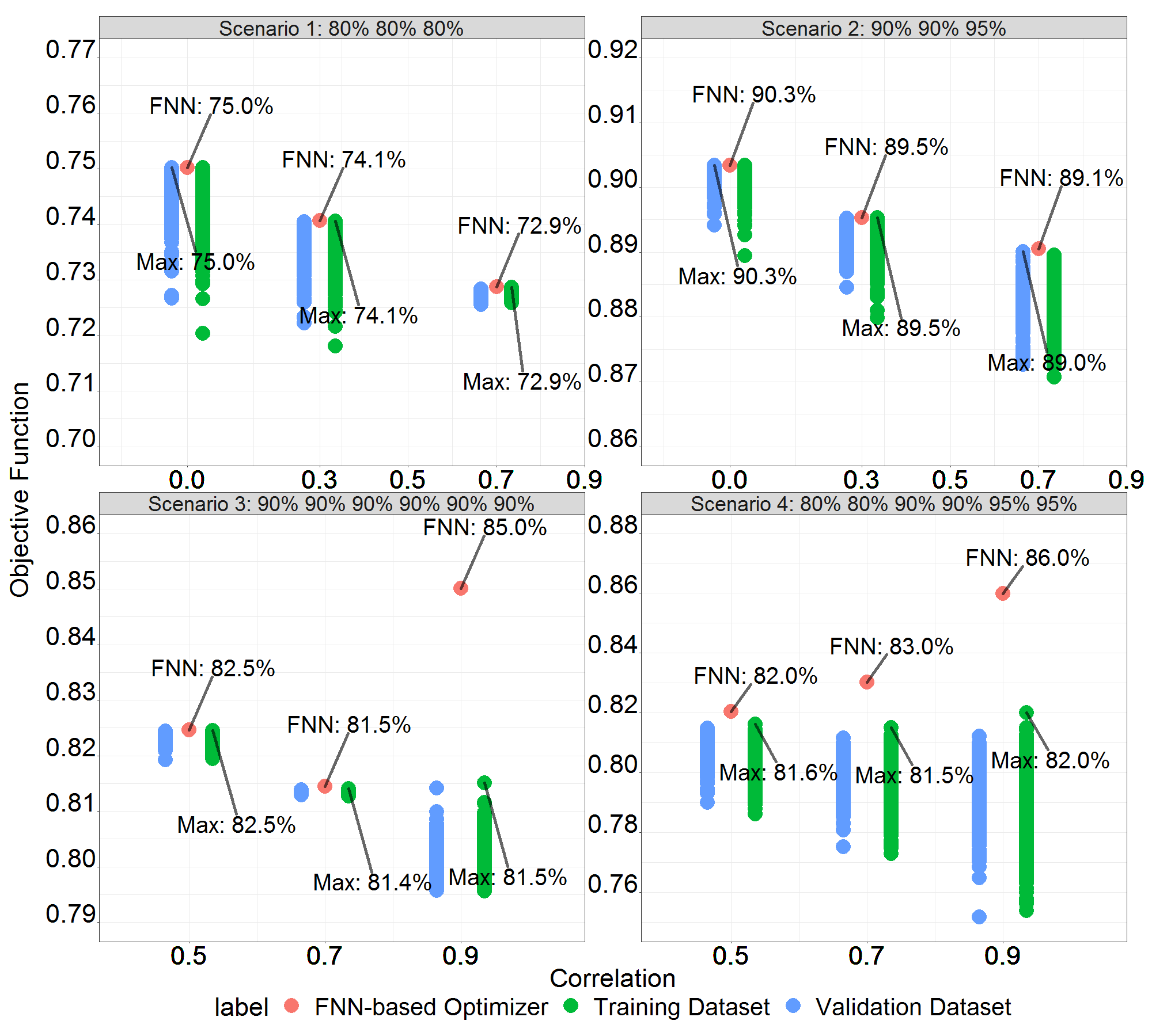
At Table 1, we summarize the optimal objective function $O\left(\boldsymbol{\alpha},T\right)$ identified by ISRES, COBYLA and the FNN-based optimizer along with their corresponding convergence times in minutes. The maximum of the optimal solutions from three methods is highlighted. The convergence time of ISRES is missing when it reaches the maximum wall time, which is the convergence time of the FNN-based optimizer multiplied by $1.5$. In all scenarios evaluated, the FNN-based method consistently identifies the optimal objective function. However, the performance of the other two methods is not stable; for example ISRES yields $74.6\%$ compared to $75.0\%$ for the rest in the first scenario with correlation $0$, and COBYLA finds $80.4\%$ compared to $86.0\%$ in scenario $4$ with correlation $0.9$. As for convergence, COBYLA is the fastest, followed by our FNN-based method, followed by ISRES. Although the FNN-based method is not the fastest, it achieves higher power than the other methods, with only a modest increase in computing time. Therefore, our FNN-based optimizer offers a better balance between time efficiency and robustness in identifying the optimal graphical approach.

Even though the gain in some cases is merely a fraction of a percent of power, it is still worth the additional computing time, which is never more than a couple of hours, especially if either the cost of the study is high or the stakes are high based on participation of subjects with serious afflictions.

We observe that ISRES performs well in Scenario 1 and 2 with three endpoints, but cannot identify the optimal value in Scenario 3 and 4 with six endpoints. In the context of a high-dimensional objective function, ISRES is far away from the optimal solution within the given wall time. When it comes to COBYLA, it is off the target in cases with equal treatment effects (Scenario 1 and 3) and lower correlations. The reason could be that COBYLA is more likely to get stuck in the local optimal under those settings.

Table 1: Optimal $O\left(\boldsymbol{\alpha},T\right)$ identified by FNN, ISRES and COBYLA

Scenario	Correlation	Optimal $O\left(\boldsymbol{\alpha},T\right)$			Convergence time (mins)
		FNN	ISRES	COBYLA	FNN	ISRES	COBYLA
1	0	75.0%	75.0%	74.6%	68.5	-	0.4
	0.3	74.1%	74.1%	73.8%	72.3	-	0.5
	0.7	72.9%	72.9%	72.9%	66.0	-	0.3
2	0	90.3%	90.3%	90.3%	67.6	-	0.3
	0.3	89.5%	89.5%	89.5%	68.5	-	0.5
	0.7	89.1%	89.1%	89.0%	68.1	-	0.4
3	0.5	82.5%	82.4%	82.4%	168.3	-	10.2
	0.7	81.5%	81.4%	81.4%	166.5	-	9.7
	0.9	85.0%	81.5%	85.0%	164.8	-	22.6
4	0.5	82.0%	81.2%	82.0%	161.3	-	10.4
	0.7	83.0%	81.0%	83.0%	163.0	-	13.3
	0.9	86.0%	80.4%	86.0%	156.1	-	12.4

We further compare our FNN-based optimizer against the brute-force searching approach in Figure 3. In each case evaluated, the left column (blue) corresponds to the validation dataset with $2,000$ graphs, and the right column (green) represents the training dataset with $8,000$ graphs. The maximum of both training and validation datasets are denoted as “Max”, which corresponds to the solution from the window-searching approach. The middle red dot is the optimal graph identified by our FNN-based optimizer. In the two cases with 3 endpoints, the optimal solution from FNN is close to that from the maximum of data. When there are 6 highly correlated endpoints, for example, with correlation 0.9 between each pair, the FNN-based method has moderate optimal power gain of approximately $4\%$ ($86.0\%$ vs $82.0\%$).

Figure 3: The optimal values identified by FNN-based optimization method and brute-force searching approach.

5 A case study

In this section, we apply our FNN-based optimizing approach to a hypothetical study with $1$ primary endpoint, denoted as $H_{1}$, and $10$ secondary endpoints, denoted as $H_{2}$ to $H_{11}$ respectively. Since the rejection of a secondary endpoint would only be meaningful when the primary endpoint is rejected, then the following objective function could be defined if all $10$ secondary endpoints are of equal importance,

$$O^{\prime}\left(\boldsymbol{\alpha},T\right)=\sum_{i=2}^{11}\frac{1}{10}\text{ E}_{\boldsymbol{p}}\left[D^{\prime}_{i}\left(\boldsymbol{\alpha},T,\boldsymbol{p}\right)\right],$$ (11)

where $D^{\prime}_{i}\left(\boldsymbol{\alpha},T,\boldsymbol{p}\right)=1$ if both $H_{i}$ and $H_{1}$ are rejected by the graphical approach $g(\boldsymbol{\alpha},T)$, and $0$ otherwise.

Since the primary endpoint is tested first, then we fix the first element in $\boldsymbol{\alpha}$ at the one-sided FWER $0.025$ and the remaining components at $0$. Therefore, $\bar{\boldsymbol{\alpha}_{b}}$ is empty. In the transition matrix $T$, $H_{1}$ could freely pass its error rate to all secondary endpoints, and each secondary endpoint could recycle theirs to the other $9$ secondary endpoints but not the primary one. A total of $9+10\times 8=89$ elements in $\bar{\boldsymbol{T}_{b}}$ have the following constraints:

$$0\leq T_{1j}\leq 1\text{ for }j\in\{2,3,...,10\},$$

$$\sum_{j\in\{2,3,...,10\}}T_{1j}\leq 1,$$

$$0\leq T_{ij}\leq 1\text{ for }i\in\{2,3,...,11\},j\in\{2,3,...,10,j\neq i\},$$

$$\sum_{j\in\{2,3,...,10,j\neq i\}}T_{ij}\leq 1\text{ for }i\in\{2,3,...,11\}.$$

Note that we exclude the adjusted power of the primary endpoint in equation (11), because the optimizer would be equivalent given the constraints on $\boldsymbol{\alpha}$ in the study setup. We further assume that the test statistics follow a multivariate normal distribution with $0.5$ as the correlation between secondary endpoints, and $0.3$ between primary and secondary endpoints. The marginal power of the primary endpoint is assumed to be $98\%$, and $96\%$, $96\%$, $92\%$, $92\%$, $88\%$, $88\%$, $84\%$, $84\%$, $80\%$ and $80\%$ for secondary endpoints. There are $10,000$ graphs and $1,000,000$ sets of $p$-values simulated.

A total of $6$ candidate FNN structures with $140$ nodes per layer are considered: $2$ layers with drop out rate at $0$, $3$ layers with rate $0$, $4$ layers with rate $0$, $2$ layers with rate $0.3$, $3$ layers with rate $0.3$, $4$ layers with rate $0.3$. Other parameters in the FNN-based optimizer, ISRES and COBYLA are the same as those from Section 3.2 and 4.

We first compare the performance of $4$ optimization methods (brute-force searching method, FNN-based optimizer, ISRES and COBYLA) in Figure 4(a). The first $8,000$ dots in green on the x-axis correspond to the objective functions from the training dataset, while the following $2,000$ are from the validation dataset. The brute-force searching method finds an optimal value at $75.51\%$, which is the maximum of those $10,000$ objective functions. The FNN-based optimizer identifies an optimal value at $76.36\%$, which is higher than $74.21\%$ from ISRES and $76.22\%$ from COBYLA. When it comes to convergence time, COBYLA takes $2.93$ hours, which is shorter than the $15.95$ from our FNN-based optimizer. This is expected since a local optimization method is generally more efficient than a global method. However, ISRES does not converge in the given time ($23.93$ hours). The residuals of FNN are plotted in Figure 4(b), with MSE $7.76\times 10^{-6}$ in training data and MSE $7.82\times 10^{-6}$ in validation data. The relatively small residuals indicate that FNN approximates the underlying objective function pretty well, and also has good generalizability.

(a)

(b)

Figure 4: (a) Objective function of $8,000$ training graphs (green), $2,000$ validation graphs (blue) and the optimal objective function identified by $4$ methods: brute-force searching method, FNN-based optimizer, ISRES and COBYLA. (b) FNN residuals in training and validation data.

6 Concluding remarks

In this manuscript, we propose an FNN-based optimization framework for the graphical procedure of multiplicity control in confirmatory clinical trials. This framework takes advantage of the strong functional representation of deep neural networks and further utilizes constraint optimization techniques to locate the solution. Simulation studies show that our FNN-based optimizer consistently identifies the optimal graph, and has a better balance between robustness and time efficiency as compared to two popular derivative-free optimization methods that could handle bound and inequality constraints.

One should acknowledge the randomness of the training data when simulated from a previous study. Consider a clinical trial with prior knowledge that each endpoint has exactly $80\%$ marginal power. Our approach would identify an optimal graph in favor of a particular endpoint, if its simulated power is higher than others. Increasing the number of simulation iterations would be helpful to stabilize the solution.

Moreover, the term “optimal graph” is with respect to the objective function defined in (3). One would not expect our identified optimal graph to have the highest multiplicity adjusted power on all endpoints compared to any other graphs. The solution would also be different if the team assigns another set of weight/importance values on endpoints in the objective function. In practice, operational factors should also be incorporated into the decision making of the final graphical procedure.

References

- [Abadi et al., 2015] Abadi, M., Agarwal, A., Barham, P., Brevdo, E., Chen, Z., Citro, C., Corrado, G. S., Davis, A., Dean, J., Devin, M., Ghemawat, S., Goodfellow, I., Harp, A., Irving, G., Isard, M., Jia, Y., Jozefowicz, R., Kaiser, L., Kudlur, M., Levenberg, J., Mané, D., Monga, R., Moore, S., Murray, D., Olah, C., Schuster, M., Shlens, J., Steiner, B., Sutskever, I., Talwar, K., Tucker, P., Vanhoucke, V., Vasudevan, V., Viégas, F., Vinyals, O., Warden, P., Wattenberg, M., Wicke, M., Yu, Y., and Zheng, X. (2015). TensorFlow: Large-scale machine learning on heterogeneous systems. Software available from tensorflow.org, https://www.tensorflow.org/.
- [Allaire and Chollet, 2018] Allaire, J. and Chollet, F. (2018). keras: R Interface to ’Keras’. R package version 2.2.0, https://CRAN.R-project.org/package=keras.
- [Allaire and Tang, 2018] Allaire, J. and Tang, Y. (2018). tensorflow: R Interface to ’TensorFlow’. R package version 1.9, https://CRAN.R-project.org/package=tensorflow.
- [Birgin and Martínez, 2008] Birgin, E. G. and Martínez, J. M. (2008). Improving ultimate convergence of an augmented Lagrangian method. Optimization Methods and Software, 23(2):177–195.
- [Bretz et al., 2009] Bretz, F., Maurer, W., Brannath, W., and Posch, M. (2009). A graphical approach to sequentially rejective multiple test procedures. Statistics in medicine, 28(4):586–604.
- [Chollet and Allaire, 2018] Chollet, F. and Allaire, J. (2018). Deep learning with R, volume 1. Manning publications.
- [Chollet et al., 2015] Chollet, F. et al. (2015). Keras. https://keras.io.
- [Conn et al., 1991] Conn, A. R., Gould, N. I., and Toint, P. (1991). A globally convergent augmented Lagrangian algorithm for optimization with general constraints and simple bounds. SIAM Journal on Numerical Analysis, 28(2):545–572.
- [Courant, 1943] Courant, R. (1943). Variational methods for the solution of problems with equilibrium and vibration. Bull. Amer. Math. Soc., 49:1–23.
- [Cybenko, 1989] Cybenko, G. (1989). Approximation by superpositions of a sigmoidal function. Mathematics of control, signals and systems, 2(4):303–314.
- [Dmitrienko et al., 2003] Dmitrienko, A., Offen, W. W., and Westfall, P. H. (2003). Gatekeeping strategies for clinical trials that do not require all primary effects to be significant. Statistics in medicine, 22(15):2387–2400.
- [Duchi et al., 2011] Duchi, J., Hazan, E., and Singer, Y. (2011). Adaptive subgradient methods for online learning and stochastic optimization. Journal of Machine Learning Research, 12(Jul):2121–2159.
- [Dugas et al., 2001] Dugas, C., Bengio, Y., Bélisle, F., Nadeau, C., and Garcia, R. (2001). Incorporating second-order functional knowledge for better option pricing. In Advances in neural information processing systems, pages 472–478.
- [Food and Drug Administration, 2017] Food and Drug Administration (2017). Multiple endpoints in clinical trials guidance for industry. https://www.fda.gov/downloads/drugs/guidancecomplianceregulatoryinformation/guidances/ucm536750.pdf.
- [Gabriel, 1969] Gabriel, K. R. (1969). Simultaneous test procedures–some theory of multiple comparisons. The Annals of Mathematical Statistics, pages 224–250.
- [Goodfellow et al., 2016] Goodfellow, I., Bengio, Y., and Courville, A. (2016). Deep learning, volume 1. MIT press Cambridge.
- [Hestenes, 1969] Hestenes, M. R. (1969). Multiplier and gradient methods. Journal of optimization theory and applications, 4(5):303–320.
- [Hinton et al., 2012] Hinton, G., Srivastava, N., and Swersky, K. (2012). Neural networks for machine learning. Coursera, video lectures, 264.
- [Hochberg, 1988] Hochberg, Y. (1988). A sharper bonferroni procedure for multiple tests of significance. Biometrika, 75(4):800–802.
- [Holm, 1979] Holm, S. (1979). A simple sequentially rejective multiple test procedure. Scandinavian journal of statistics, pages 65–70.
- [Hommel, 1988] Hommel, G. (1988). A stagewise rejective multiple test procedure based on a modified bonferroni test. Biometrika, 75(2):383–386.
- [Hornik, 1991] Hornik, K. (1991). Approximation capabilities of multilayer feedforward networks. Neural networks, 4(2):251–257.
- [Johnson, 2007] Johnson, S. G. (2007). The nlopt nonlinear-optimization package. http://ab-initio.mit.edu/nlopt.
- [Karush, 1939] Karush, W. (1939). Minima of functions of several variables with inequalities as side constraints. Master’s Thesis, Department of Mathematics, University of Chicago, Chicago.
- [Kramer et al., 2011] Kramer, O., Ciaurri, D. E., and Koziel, S. (2011). Derivative-free optimization. In Computational optimization, methods and algorithms, pages 61–83. Springer.
- [Kuhn and Tucker, 1951] Kuhn, H. W. and Tucker, A. W. (1951). Nonlinear programming. In Proceedings of the Second Berkeley Symposium on Mathematical Statistics and Probability, pages 481––492. Berkeley, Calif. University of California Press.
- [Lu et al., 2017] Lu, Z., Pu, H., Wang, F., Hu, Z., and Wang, L. (2017). The expressive power of neural networks: A view from the width. In Advances in Neural Information Processing Systems, pages 6231–6239.
- [Marcus et al., 1976] Marcus, R., Eric, P., and Gabriel, K. R. (1976). On closed testing procedures with special reference to ordered analysis of variance. Biometrika, 63(3):655–660.
- [Nair and Hinton, 2010] Nair, V. and Hinton, G. E. (2010). Rectified linear units improve restricted boltzmann machines. In Proceedings of the 27th international conference on machine learning (ICML-10), pages 807–814.
- [Nocedal and Wright, 2006] Nocedal, J. and Wright, S. J. (2006). Nonlinear Equations. Springer.
- [Powell, 1969] Powell, M. J. (1969). A method for nonlinear constraints in minimization problems. Optimization, pages 283–298.
- [Powell, 1994] Powell, M. J. (1994). A direct search optimization method that models the objective and constraint functions by linear interpolation. In Advances in optimization and numerical analysis, pages 51–67. Springer.
- [Rohmeyer and Klinglmueller, 2018] Rohmeyer, K. and Klinglmueller, F. (2018). gMCP: Graph Based Multiple Test Procedures. R package version 0.8-14, https://cran.r-project.org/package=gMCP.
- [Runarsson and Yao, 2005] Runarsson, T. P. and Yao, X. (2005). Search biases in constrained evolutionary optimization. IEEE Transactions on Systems, Man, and Cybernetics, Part C (Applications and Reviews), 35(2):233–243.
- [Simes, 1986] Simes, R. J. (1986). An improved bonferroni procedure for multiple tests of significance. Biometrika, 73(3):751–754.
- [Tamhane and Gou, 2018] Tamhane, A. C. and Gou, J. (2018). Advances in p-value based multiple test procedures. Journal of biopharmaceutical statistics, 28(1):10–27.
- [Westfall and Krishen, 2001] Westfall, P. H. and Krishen, A. (2001). Optimally weighted, fixed sequence and gatekeeper multiple testing procedures. Journal of Statistical Planning and Inference, 99(1):25–40.
- [Wiens, 2003] Wiens, B. L. (2003). A fixed sequence bonferroni procedure for testing multiple endpoints. Pharmaceutical Statistics: The Journal of Applied Statistics in the Pharmaceutical Industry, 2(3):211–215.
- [Ypma, 2018] Ypma, J. (2018). nloptr: R Interface to NLopt. R package version 1.2.1, https://cran.r-project.org/web/packages/nloptr/index.html.