Navigation of a Quadratic Potential with
Ellipsoidal Obstacles

Abstract

Given a convex quadratic potential of which its minimum is the agent’s goal and a Euclidean space populated with ellipsoidal obstacles, one can construct a Rimon-Koditschek (RK) artificial potential to navigate. Its negative gradient attracts the agent toward the goal and repels the agent away from the boundary of the obstacles. This is a popular approach to navigation problems since it can be implemented with local spatial information that is acquired during operation time. However, navigation is only successful in situations where the obstacles are not too eccentric (flat). This paper proposes a modification to gradient dynamics that allows successful navigation of an environment with a quadratic cost and ellipsoidal obstacles regardless of their eccentricity. This is accomplished by altering gradient dynamics with a Hessian correction that is intended to imitate worlds with spherical obstacles in which RK potentials are known to work. The resulting dynamics simplify by the quadratic form of the obstacles. Convergence to the goal and obstacle avoidance is established from almost every initial position (up to a set of measure one) in the free space, with mild conditions on the location of the target. Results are corroborated empirically with numerical simulations.

footnoteinfo]Department of Electrical and Systems Engineering at the University of Pennsylvania

, ,

1 Introduction

Path planning, sometimes formulated as reaching the minimum of a potential function from a start configuration while avoiding collisions with obstacles, is a cornerstone problem in controls and robotics (LaValle, 2006, Bhattacharya et al., 2007, Murphy et al., 2008). In this paper we develop a navigation function approach that is guaranteed to reach the minimum of an arbitrary quadratic convex potential in a space with an arbitrary number of ellipsoidal obstacles of arbitrary eccentricity.

To better explain this contribution it is important to emphasize that navigation function approaches to path planning occupy an appealing middle ground in terms of complexity and quality of trajectories (Rimon and Koditschek, 1992, Loizou, 2017, Vrohidis et al., 2018, Tanner and Kumar, 2005, Ghaffarkhah and Mostofi, 2009, Paternain and Ribeiro, 2019). In one extreme, bug algorithms follow potential gradients until they hit border obstacles, at which point they follow the border until the projection of the direction to the destination on the obstacle’s tangent plane pushes it away (Taylor and LaValle, 2009). Bug algorithms rely on simple local sensing of gradients and obstacles and are guaranteed to reach the target destination. But they may do so by following excessively long trajectories. In the other extreme, minimum path length search algorithms such as A^∗ (Hart et al., 1968) and random trees (LaValle, 1998) build graphs that describe the geometry of the environment and find trajectories of optimal length. But to do so they require access to complex global sensing of the environment.

Navigation function approaches combine the goal potential with repulsive potentials that push the agent away from the obstacles. This implies they can still be implemented with local sensing of gradients and obstacles while empirical evidence shows they find trajectories to the goal that are better than obstacle following bug algorithms (Loizou, 2017, Vrohidis et al., 2018, Tanner and Kumar, 2005, Ghaffarkhah and Mostofi, 2009, Paternain and Ribeiro, 2019). The cost to pay for this appealing tradeoff between sensing complexity and trajectory length is the possibility of failure. Locally implementable navigation functions are guaranteed to reach the goal, but they are difficult to construct except for conservative geometries. Famously, they are known to work always for spherical potentials in worlds with spherical obstacles (Koditschek and Rimon, 1990). With the addition of an analytic switch, local diffeomorphisms can be constructed to enable navigation of a single point agent in star worlds (Rimon and Koditschek, 1992). Since then, there has been a significant effort to implement navigation functions locally without a diffeomorphism (Paternain et al., 2018, Tanner and Kumar, 2005, Loizou, 2012). Such constructions extend the applications to to multiple agents (Dimarogonas and Johansson, 2008), non-point agents (Arslan and Koditschek, 2016), and minimal adjustment of a single tuning parameter (Lionis et al., 2008). All of these efforts, however, require that the obstacles are sufficiently curved (Filippidis and Kyriakopoulos, 2012). In the specific case of ellipsoidal obstacles, this puts a limit on their eccentricity.

More recently, Vasilopoulos et al. (2020) have shown a method to construct a diffeomporphism via polygonal decomposition on-the-fly with non-convex obstacles using real-time perception; however, they require the shape of the obstacles to be ”familiar” or come from a known obstacle class. Indeed, mapped model space after applying the diffeomporphism does need to satisfy the sufficiently curved condition.

In this work, we consider ellipsoidal worlds with arbitrary eccentricity. By drawing connections to second order optimization (Boyd and Vandenberghe, 2004, Ch. 9), we directly propose dynamics given by a Hessian correction on the locally implementable navigation function of Paternain et al. (2018). The correction on the quadratic obstacles simplifies so that the agent only requires easily obtainable information; namely, the agent must estimate the direction to the goal and obstacle centers as well as the distances to the obstacles and goal. Implementable in practice (Li and Griffiths, 2004, Fitzgibbon et al., 1999), we show that with these four quantities and with mild conditions on the position of the target, the agent is guaranteed to reach the target from almost all starting conditions while avoiding obstacles along the way.

The paper is organized as follows. In section 2, we formally introduce the path planning problem and the navigation function approach. In section 3, we present our Hessian-corrected and simplified dynamics. Following the proof of the main result in section 4, numerical results are presented in section 5 which showcases the success in spaces where the traditional navigation function approaches fail. We conclude in section 6 with a summary and possible extensions of this work.

2 Potential, Obstacles, & Navigation Functions

We consider the problem of a point agent navigating a quadratic potential in a space with ellipsoidal punctures. Formally, let $\mathcal{X}\subset{\mathbb{R}}^{n}$ be a non empty compact convex domain that we call the workspace, and let ${f_{0}}:{\mathcal{X}}\to{\mathbb{R}}_{+}$ be a convex strictly quadratic function that we call the potential. A point agent is interested in reaching the target destination $x^{*}\in{\mathcal{X}}$ which is defined as the minimizer of the potential. Without loss of generality, we use the standard squared Euclidean distance to the target

$$x^{*}=\operatornamewithlimits{argmin}_{x\in{\mathcal{X}}}{f_{0}}(x):=\frac{1}{2}\|x-x^{*}\|^{2}.$$ (1)

In some navigation problems, arbitrary quadratic functions are of interest (Paternain et al., 2018). For future reference, we denote the minimum and maximum eigenvalues of $Q:=\nabla^{2}{f_{0}}(x)$ as $0<\lambda_{\textrm{min}}\leq\lambda_{\textrm{max}}$.

The workspace ${\mathcal{X}}$ is populated by $m$ ellipsoidal obstacles ${\mathcal{O}}_{i}\subset{\mathcal{X}}$ for $i=1,\dots,m$ which are closed and have a non empty interior. We define the free space as the complement of the obstacle set relative to the workspace,

$${\mathcal{F}}:={\mathcal{X}}\ \backslash\ \Big(\,{\textstyle\bigcup\limits_{i=1}^{m}}{\mathcal{O}}_{i}\,\Big),$$ (2)

We assume that each obstacle, or each connected component of the complement of the workspace is an ellipsoid. Formally, we have the assumption

Assumption 1

Obstacles are ellipsoids. Each obstacle is represented as the zero sublevel set of a proper convex quadratic function $\beta_{i}:{\mathbb{R}}^{n}\to{\mathbb{R}}$

$$\beta_{i}(x)=\frac{1}{2}(x-x_{i})^{\top}A_{i}(x-x_{i})-\frac{1}{2}r_{i}^{2},$$ (3)

where $A_{i}$ is a positive definite matrix with minimum and maximum eigenvalues $0<\mu^{i}_{\textrm{min}}\leq\mu^{i}_{\textrm{max}}$, $x_{i}$ is the ellipsoid center and $r_{i}$ is the maximum axis length so that

$${\mathcal{O}}_{i}=\left\{x\in{\mathcal{X}}{\,\big|\,}\beta_{i}(x)\leq 0\right\}.$$ (4)

From (3) and (4) it follows that ${\mathcal{O}}_{i}$ is an ellipsoid centered at $x_{i}$ with axes given by the eigenvectors of $A_{i}$. The length of the axis along the $k$th eigenvector is $r_{i}\mu^{i}_{k}$. In particular, the length of the minor axis is $r_{i}\mu^{i}_{\textrm{min}}$ and the length of the major axis is $r_{i}\mu^{i}_{\textrm{max}}$.

While it is true that convergence guarantees have been given for more complex obstacles, such as tori, cylinders, one-sheet hyperboloids, and convex obstacles in general Filippidis and Kyriakopoulos (2012), Paternain et al. (2018), these obstacles must be sufficiently curved. In the case of ellipsoidal obstacles, this puts a restriction on their eccentricity. Focusing on the ellipsoidal case, this work guarantees convergence on ellipsoidal worlds with arbitrary eccentricity.

We further introduce a concave quadratic function $\beta_{0}:{\mathbb{R}}^{n}\to{\mathbb{R}}$ so that we write the workspace as a superlevel set,

$${\mathcal{X}}=\left\{x\in{\mathbb{R}}^{n}{\,\big|\,}\beta_{0}(x)\geq 0\right\}.$$ (5)

The fact that the workspace is bounded admits the following bounds which will appear in our convergence analysis. Let $B$ be a strictly positive constant. For any four points $a,b,c,d\in{\mathcal{X}}$, the absolute value of the inner product of the distances $a-b$ and $c-d$ is bounded by

$$|(a-b)^{\top}(c-d)|\leq B.$$ (6)

Additionally, let

$$\Lambda_{0}:=\max_{i,x\in{\mathcal{X}}}\beta_{i}(x),~\textrm{and}~P_{0}:=\max_{x\in{\mathcal{X}}}{f_{0}}(x).$$ (7)

The navigation problem we want to solve is one in which the agent stays in the interior of the workspace at all times, does not collide with any obstacle, and approaches the goal at least asymptotically.

For a formal specification we specify the agent’s goal as that of finding a trajectory $x(t)$ such that for all $t\geq 0$,

$$x(t)\in{\mathcal{F}},~\textrm{and}~\lim_{t\to\infty}x(t)=x^{*}.$$ (8)

The problem is feasible when $x^{*},x(0)\in\mathcal{F}$.

2.1 Navigation Functions

A navigation function is a twice continuously differentiable function defined on the free space that satisfies three properties: (i) It has a unique minimum at $x^{*}$. (ii) All of its critical points are are nondegenerate. (iii) Its maximum is attained at every point on the boundary of the free space. These three properties guarantee that if an agent follows the negative gradient of the navigation function, it will converge to the minimum of the navigation function without running into the boundary of free space for almost every initial condition (Koditschek and Rimon, 1990). Thus, it is possible to recast (8) as the problem of finding a navigation function whose minimum is at the goal destination $x^{*}$. This is always possible to do since for any manifold with boundary it is guaranteed that such a function exists (Rimon and Koditschek, 1992). In practice, depending on the geometry of the freespace the navigation functions are constructed differently. For instance, in sphere worlds, Rimon-Koditschek artificial potentials can be used (Rimon and Koditschek, 1992), and in topologically complex ones navigation functions based on harmonic potentials are preferred (Loizou, 2011, Loizou, 2012). The family of Rimon-Koditshek potentials was extended to enable the navigation of convex potentials in a space of convex obstacles (Filippidis and Kyriakopoulos, 2012, Paternain et al., 2018, Rimon and Koditschek, 1991). However, some geometric conditions restrict its application directly, which we will now elucidate.

The Rimon-Koditschek navigation function is formally defined by $\varphi_{k}:{\mathcal{F}}\to{\mathbb{R}}_{+}$ with parameter $k\in\mathbb{R}$ as

$$\varphi_{k}(x)=\frac{{f_{0}}(x)}{\left({f_{0}}^{k}(x)+\beta_{0}(x)\beta(x)\right)^{1/k}},$$ (9)

where the function $\beta:{\mathbb{R}}^{n}\to{\mathbb{R}}$ is the product of all the obstacle equations,

$$\beta(x)=\prod_{i=1}^{m}\beta_{i}(x).$$ (10)

It was established that $\varphi_{k}(x)$ is a navigation function when $k$ is sufficiently large under some restrictions on the shape of the obstacles, the potential function, and position of the goal (Filippidis and Kyriakopoulos, 2012, Paternain et al., 2018).

Namely, $\varphi_{k}(x)$ in (9) is not always a valid navigation function because for some geometries it can have several local minima as critical points for all $k>0$. For the case of a quadratic potential and ellipsoidal obstacles that we consider here, a sufficient condition for $\varphi_{k}(x)$ to be a valid potential is when (Paternain et al., 2018, Theorem 3)

$$\frac{\lambda_{\textrm{max}}}{\lambda_{\textrm{min}}}\times\frac{\mu^{i}_{\textrm{max}}}{\mu^{i}_{\textrm{min}}}<1+\frac{d_{i}}{r_{i}\mu^{i}_{\textrm{max}}},$$ (11)

where $d_{i}=\|x_{i}-x^{*}\|$ is the distance from the center of the ellipsoid to the goal. When (11) fails, $\varphi_{k}$ might fail to be a navigation function because it may present a local minimum on the side of the obstacle opposite the target.

An important consequence of (11) is that the artificial potential $\varphi_{k}(x)$ in (9) may fail to solve the navigation problem specified in (8). Indeed, it will fail whenever the obstacles are wide with respect to the potential level sets. On the other hand, notice that when the attractive potential is rotationally symmetric and the obstacles are spherical, the left hand side of the previous expression is equal to one, and thus the condition is always satisfied. The main contribution of this paper is to leverage this observation as a motivation for introducing a correction to the gradient field of an Rimon-Koditschek navigation function that results in a field construction that is valid in all environments with ellipsoidal obstacles, and for any quadratic potential.

3 Curvature Corrected Navigation Fields

To gain some intuition about the gradient-following dynamics of Rimon-Koditschek potentials we write them explicitly as

$$\begin{split}\dot{x}&=-\nabla\varphi_{k}\\ &=-\left(f_{0}^{k}+\beta\beta_{0}\right)^{-1-\frac{1}{k}}\left(\beta\beta_{0}\nabla{f_{0}}-\frac{{f_{0}}\nabla(\beta\beta_{0})}{k}\right).\end{split}$$ (12)

Note that for convenience in notation, we omit the dependence on $x$. In practice, the dynamics are typically normalized since the norm of the gradient is generally small (Whitcomb and Koditschek, 1991). Therefore, it is reasonable to omit the scaling $(f_{0}^{k}+\beta\beta_{0})^{-1-1/k}$. We also omit $\beta_{0}$ for simplicity, a minor modification which we explain in Section 4.1. The resulting dynamics is

$$\dot{x}=g_{\textrm{nav}}(x):=-\beta\nabla{f_{0}}+\frac{{f_{0}}}{k}\nabla\beta.$$ (13)

The first term, $-\beta\nabla{f_{0}}$, in this dynamical system is a potential field attracting the agent to the goal, and the second term, $({f_{0}}/k)\nabla\beta$, is a repulsive field pushing the agent away from the obstacles. When the agent is close to the obstacle ${\mathcal{O}}_{i}$, the product function $\beta$ takes a value close to zero thereby eliminating the first summand in (13) and prompting the agent’s velocity to be almost collinear with the vector $\nabla\beta(x)$. In turn, this makes the time derivative $\dot{\beta}(x)$ positive thus preventing $\beta(x)$ from becoming negative. This guarantees that the agent remains in free space. When the agent is away from the obstacles, the term that dominates is the negative gradient of $f_{0}(x)$ which pushes the agent towards the goal $x^{*}$. The parameter $k$ balances the relative strengths of these two potentials.

At points where the attractive and repulsive potentials cancel we find critical points. By choosing large enough $k$, these points can be made into saddles when (11) holds. An important observation here is that the condition is always satisfied when the potential and the obstacles are spherical because in that case the left hand side is $(\lambda_{\textrm{max}}/\lambda_{\textrm{min}})\times(\mu^{i}_{\textrm{max}}/\mu^{i}_{\textrm{min}})=1$. This motivates an approach in which we implement a change of coordinates to render the geometry spherical. The challenge is that the change of coordinates that would render one obstacle spherical is not the same change of coordinates that would render the potential, or any of the other obstacles, spherical. Still, this idea motivates the curvature-corrected dynamics that we present in this section. We emphasize that this exposition is only meant to motivate introducing the navigation dynamics developed in this paper. At no point during implementation does the agent need to estimate the Hessians of the obstacles.

3.1 Proposed Navigation Dynamics

Consider the obstacle gradient term $\nabla\beta$ from (13). Use the product rule of derivation to write

$$\nabla\beta=\sum_{i=1}^{m}\bar{\beta}_{i}\nabla\beta_{i},~~\bar{\beta}_{i}\triangleq\prod_{j\neq i}\beta_{j}.$$ (14)

Apply separate correction terms to the gradient of each obstacle function ($\nabla^{2}\beta_{i}^{-1}\beta_{i}$), which simplifies to $x-x_{i}$ as well as the potential function ($\nabla^{2}{f_{0}}^{-1}{f_{0}}$), which simplifies to $x-x^{*}$. Our proposed dynamics therefore becomes

$$\dot{x}=g_{\textrm{new}}(x):=-\beta\cdot(x-x^{*})+\frac{{f_{0}}(x)}{k}\sum_{i=1}^{m}\bar{\beta}_{i}\cdot(x-x^{i}).$$ (15)

Similar to how Newton’s Method uses second order information to render the level sets of the objective function into spherical sets so to obtain a faster rate of convergence(Boyd and Vandenberghe, 2004, Ch. 9.5), pre-multiplying each gradient in the original flow (13) by the Hessian inverse of the corresponding function corrects the dynamics so that the world appears spherical to the agent.

An interesting side effect of the simplified dynamics expression in (15) is that implementation is simpler than it appears. The first term pushes in the direction of the goal and the second term pushes away from the center of the obstacle. Thus, the algorithm can be made to work if we just estimate these two quantities. Curvature estimates are not needed for implementation.

The advantages of this approach are threefold: (i) the estimate of the Hessian does not need to be computed, (ii) the dynamics are simpler and easier to implement, and (iii) the convergence proof is complete for almost all initial conditions $x_{0}$ (with measure one) with mild conditions on the location of the target. We now present our main result, which guarantees convergence to the target in environments with ellipsoidal obstacles.

3.2 Convergence Guarantees

Before we present our main result, we require the following definitions. Because the obstacles are ellipsoidal, and the target is a point, for each obstacle, we define the generalized Voronoi cell (Arslan and Koditschek, 2016) based on maximum margin separating hyperplanes to be

$$\mathcal{C}_{i}:=\left\{x\in{\mathcal{F}}\bigg|\forall_{j\neq i}\forall_{p\in{\mathcal{O}}_{i}}\forall_{q\in{\mathcal{O}}_{j}}\|x-p\|\leq\|x-q\|\right\},$$ (16)

for all $i,j=1,\dots,m$ where we define ${\mathcal{O}}_{0}:=x^{*}$. For each Voronoi cell $\mathcal{C}_{i}$, we can define its boundary to an adjacent cell $\mathcal{C}_{j}$ by

$$\partial\mathcal{C}_{i}^{j}:=\left\{x\in\mathcal{C}_{i}\bigg|\forall_{p\in{\mathcal{O}}_{i}}\forall_{q\in{\mathcal{O}}_{j}}\|x-p\|=\|x-q\|\right\}.$$

We also assume that the target is bounded away from the union of the affine extension of the Voronoi borders. Formally, we assume the following.

Assumption 2

Target lies away from hyperplanes For each $\partial{\mathcal{C}}_{i}^{j}$, there exists a $\delta_{i,j}>0$ such that the inner product between $(x-x*)$ and the normal unit vector perpendicular to $\partial{\mathcal{C}}_{i}^{j}$, or ${\mathbf{n}}_{i,j}$, is strictly positive. In particular, for any $a,b,x\in\partial{\mathcal{C}}_{i}^{j}$, the normal vector ${\mathbf{n}}_{i,j}$ satisfies

$${\mathbf{n}}_{i,j}^{\top}(a-b)=0,\textrm{and~}{\mathbf{n}}_{i,j}^{\top}(x-x^{*})>0,$$ (17)

and

$${\mathbf{n}}_{i,j}^{\top}(x-x^{*})\geq\delta_{i,j}.$$ (18)

Assumption 2 simplifies the analysis significantly, albeit at the cost of placing minor conditions on the location of the target. We discuss the procedure to lift these conditions in Remark 1. We are now equipped to present our main result.

Theorem 1

Let ${f_{0}}(x)$ be a quadratic potential as in (1) and let $\beta_{i}(x)$ be an ellipsoid as in (3) for all $i=1,\dots,m$. Further let $x$ be the solution of the dynamical system (15) with initial condition $x_{0}$, and let Assumption 2 be in effect. Then, there exists a $K$ such that when $k>K$, $x(t)\in{\mathcal{F}}$ for all $t\geq 0$ and $\lim_{t\to\infty}x(t)=x^{*}$ for almost all initial conditions $x_{0}$.

The complete proof is presented in section 4, however we present a sketch of proof here.

• First, we show that the free space ${\mathcal{F}}$ is invariant (Section 4.1).

• Then, we show that the dynamics (15) induce a directed acyclic graph which determines the order in which the Voronoi cells defined in (16) are traversed. The final cell visited is a cell containing the target. (Section 4.2 and Section 4.3).

• Furthermore, we show that $x^{*}$ is stable in ${\mathcal{C}}_{0}$, the Voronoi cell containing the target. (Section 4.4)

• Finally, we show that the agent will almost always exit each Voronoi cell ${\mathcal{C}}_{i}$, $i=1,\dots,m$. (Section 4.5)

The order of the bullets is selected intentionally. To prove bullet three, we use a Lyapunov function. Together with the invariance of the final ${\mathcal{C}}_{0}$, it follows that $x^{*}$ is asymptotically stable. In order to show the final bullet of the proof, we invoke the same Lyapunov function of bullet three in specific regions where we know how the obstacle will traverse the border of those sets. In particular, we use the Lyapunov function to show that the agent will leave that specified set.

Remark 1

Notice that $\partial{\mathcal{C}}_{i,j}$ are contained in an affine hyperplane. For the purpose of this remark, let $\partial{\mathcal{C}}_{i,j}$ be the affine extension of the border between two adjacent cells. The analysis holds for all configurations except for the case where the target lies on the set with zero measure of the union of the affine hyperplanes $\cup_{i,j}\partial{\mathcal{C}}_{i,j}$, albeit with arbitrarily high $K$. For that reason, we introduce Assumption 2 so that we can find a bounded $K$. Theoretically, one should be able to obtain a finite value of $k$ without Assumption 2 by treating the union of adjacent cells where the border is aligned with $(x-x^{*})$ as one cell. In practice, one can consider perturbing the target location within ${\mathcal{C}}_{0}$ until Assumption 2 holds and returning to the original target location when the agent is sufficiently close. As such, we choose to omit this formal discussion because these are corner cases, and they have no effect on the performance in practice.

4 Proof of Theorem 1

In this section, we present the proof of Theorem 1. Let $N_{r}(A)\triangleq\bigcup_{p\in A}B_{r}(p)$, where $B_{r}(p)\triangleq\{q\colon\|q-p\|<r\}$ be the open $r$-neighborhood of a set $A$. Further, consider a subset of the free space outside the $\varepsilon$-neighborhood of any obstacle, namely,

$$\mathcal{F}_{>\varepsilon}:=\mathcal{F}\backslash\bigcup_{i}N_{\varepsilon}(\mathcal{O}_{i}).$$ (19)

4.1 Invariance of the workspace

The following Lemma explains why it is possible to omit $\beta_{0}$ from the dynamics in (15). We define the following constants

$$\lambda=\min_{i,x\in\cup_{i,j}\partial{\mathcal{C}}_{i,j}}\beta_{i},~~~\lambda_{0}=\min_{i,x\in\partial{\mathcal{X}}}\beta_{i}.$$ (20)

Lemma 1

Let $K_{\beta_{0}}=mP_{0}\Lambda_{0}^{m-1}B/\lambda_{0}^{m}$, where the $m$ is the number of obstacles and the constants $P_{0},\Lambda_{0},\lambda_{0},$ and $B$ come from (7), (20), and (6). For $k>K_{\beta_{0}}$, ${\mathcal{F}}$ is invariant under (15).

Proof 4.2.

First consider the boundary of an obstacle $\partial\mathcal{O}_{i}$, for $i=1,\dots,m$. Evaluate $\nabla\beta_{i}^{\top}\dot{x}$ with $\dot{x}$ subject to $\beta_{i}=0$. We obtain

$$\nabla\beta_{i}^{\top}\dot{x}\Big|_{\beta_{i}=0}=\frac{{f_{0}}}{k}\nabla\beta_{i}^{\top}(x-x^{i}),$$ (21)

which is strictly positive by $\mu_{\min}^{i}>0$.

Next, consider the outer obstacle. Without loss of generality, let $\nabla^{2}\beta_{0}=I_{n}$. Consider the normal vector ${\mathbf{n}}=(x-x^{*})/\|x-x^{*}\|$. Evaluate ${\mathbf{n}}^{\top}\dot{x}$ to obtain

$${\mathbf{n}}^{\top}\dot{x}=-\beta+\frac{{f_{0}}}{k}\sum_{i=1}^{m}\bar{\beta}_{i}\cdot{\mathbf{n}}^{\top}(x-x_{i}).$$ (22)

Recalling the bounds (6) and (7), ${\mathbf{n}}^{\top}\dot{x}$ is strictly negative when $k>K_{\beta_{0}}$ defined by

$$K_{\beta_{0}}:=\frac{mP_{0}\Lambda_{0}^{m-1}B}{\lambda_{0}^{m}}.$$ (23)

We invoke Nagumo’s Theorem (Blanchini, 1999) to complete the proof.

4.2 Isolating obstacles analysis with Voronoi cells

Figure 1: Visualization of the different regions of the spaces described in the proof. The red region around the obstacle in black is the $\varepsilon$ neighborhood of the obstacle. The green dashed lines and the green cylinder define the pyramid and cylinder discussed in Section 4.5. The blue line describes $S_{i}$, which attracts the points in the Voronoi cell whose borders shown by the dashed gray lines.

Recall from Assumption 2 that ${\mathbf{n}}_{i,j}$ is a unit vector perpendicular to the border $\partial{\mathcal{C}}_{i,j}$ such that ${\mathbf{n}}_{i,j}^{\top}(x-x^{*})>\delta_{i,j}$ for some positive $\delta_{i,j}>0$. Our next lemma establishes a relative ordering on adjacent obstacles.

Lemma 4.3.

Let Assumption 2 hold. Further, let $K_{i,j}=mP_{0}\Lambda_{0}^{m-1}B\delta_{i,j}^{-1}\lambda^{-m}$, where $m$ is the number of obstacles and the constants $P_{0}$, $\Lambda_{0}$, $\lambda$, $B$, and $\delta_{i,j}$ come from (7), (20), (6), and Assumption 2. Then, for all $k>K_{i,j}$, ${\mathbf{n}}_{i,j}^{\top}\dot{x}<0$.

Proof 4.4.

Evaluate $n^{\top}\dot{x}$

$${\mathbf{n}}^{\top}\dot{x}=-\beta{\mathbf{n}}^{\top}(x-x^{*})+\frac{f_{0}}{k}\sum_{j=1}^{m}\bar{\beta}_{j}{\mathbf{n}}^{\top}(x-x_{i}).$$ (24)

By the definition of the Voronoi cell, $\partial C_{i}^{j}$ does not intersect with any obstacle. Invoke (6), (7), and (20) to obtain the bound

$$\beta{\mathbf{n}}^{\top}(x-x^{*})\geq\delta_{i,j}\lambda^{m}.$$ (25)

We also bound the expression

$${f_{0}}\sum_{j=1}^{m}\bar{\beta}_{j}{\mathbf{n}}^{\top}(x-x_{j})\leq mP_{0}\Lambda_{0}^{m-1}B.$$ (26)

Using these bounds, we define

$$K_{i,j}:=\frac{mP_{0}\Lambda_{0}^{m-1}B}{\delta_{i,j}\lambda^{m}}.$$ (27)

It holds that ${\mathbf{n}}^{\top}\dot{x}$ is negative for all $k>K_{i,j}$

In fact, for any hyperplane section that is $\varepsilon$-bounded away from the targets, we can establish a similar traversal property. We formalize this with the following corollary.

Corollary 4.5.

Let ${\mathcal{H}}$ be a hyperplane section that is contained in ${\mathcal{F}}_{>\varepsilon}$. Let $n$ be a normal vector to the hyperplane section such that ${\mathbf{n}}^{\top}(x-x^{*})>\delta$ for some $\delta>0$ and for any $a,b\in{\mathcal{H}}$, $n^{\top}(a-b)=0$. Then for any $k>mP_{0}\Lambda_{0}^{m-1}B\delta^{-1}\lambda^{m}$, it holds that ${\mathbf{n}}^{\top}\dot{x}<0$ for the flow given in (15).

Proof 4.6.

The proof follows identically from Lemma 4.3.

Lemma 4.3 induces a relative ordering on adjacent obstacles. Indeed, this ordering is such that once an agent leaves the Vornonoi cell of an obstacle ${\mathcal{O}}_{i}$, it will never return to that cell. Eventually, the agent will be in ${\mathcal{C}}_{0}$ where it will converge to the target (see Section 4.4). We will first formally define the ordering, then we will prove the claim.

4.3 Ordering on the obstacles

We will construct the ordering $\rho(0),\dots,\rho(m)$ on the Voronoi cells $\mathcal{C}_{i}$, for $i=0,\dots,m$. First assign 0 to $\rho(0)$, that is the Voronoi cell containing the target.

Next, define the Voronoi cells for the remaining obstacles $\mathcal{C}_{i}(\ell)$, where $\ell$ denotes the number of obstacles removed. For brevity in notation, we let $\rho_{\ell}$ denote $\left\{\rho(i)\right\}_{i=0}^{\ell}$. We define

$$\mathcal{C}_{i}(\ell):=\left\{x\in{\mathcal{F}}\bigg|\forall_{j\notin\rho_{\ell}\atop j\neq i}\forall_{p\in{\mathcal{O}}_{i}}\forall_{q\in{\mathcal{O}}_{j}}\|x-p\|\leq\|x-q\|\right\}.$$ (28)

Where $\mathcal{C}_{i}(\ell)$ is defined only for $i=1,\dots,m$ such that $i\notin\rho_{\ell}$ and $\ell=0,\dots,m-2$. By Assumption 2, there exists an $i\notin\rho_{\ell}$ such that $x^{*}\in\mathcal{C}_{i}(\ell)$. Assign this $i$ to $\rho(\ell+1)$. This process is repeated for all $\ell$ until there are are just two cells. Assign $i\notin\rho_{m-1}$ to $\rho(m)$ to complete the ordering. This process is shown visusally in Figure 2.

(a)	(b)	(c)

Figure 2: Let the red $*$ represent the location of the target. (a) The cell containing the target is invariant by Lemma 4.3, as shown with the dashed border. The red cell is the next obstacle we will add to the invariant set. (b) Consider removing the yellow cell from Fig 2a, and reconstruct the Voronoi diagram. The obstacle lies in the new Voronoi cell corresponding to the red Voronoi cell. The dashed borders are the same in the original Voronoi diagram, and by Lemma 4.3, the agent can only enter the red cell from the white neighboring cells. (c) As shown in Lemma 4.7, the union of the two cells is invariant.

The following lemma establishes that the union $\cup_{i=0}^{n}\mathcal{C}_{\rho(i)}$ is invariant for all $n=0,\dots,m$.

Lemma 4.7.

Let $K_{\rho}=\max_{i,j}K_{i,j}$, where $K_{i,j}$ is defined as in (27). Let $\rho$ be the ordering defined in Section 4.3. Then, for all $k>K_{\rho}$, it holds that $\cup_{i=0}^{n}{\mathcal{C}}_{\rho(i)}$ is invariant under the flow (15) for all $n=0,\dots,m$.

Proof 4.8.

We prove the lemma by induction. That ${\mathcal{C}}_{0}$ is invariant comes directly from applying Lemma 4.3 on $\partial{\mathcal{C}}_{0}$ via Nagumo’s Theorem (Blanchini, 1999).

Next, we will establish that

$${\mathcal{C}}_{\rho(\ell+1)}(\ell)\cup\left(\cup_{i=0}^{\ell}{\mathcal{C}}_{\rho(i)}\right)=\cup_{i=0}^{\ell+1}{\mathcal{C}}_{\rho(i)}.$$ (29)

It suffices to show equivalence on the set difference

$$\begin{split}{\mathcal{C}}_{\rho(\ell+1)}(\ell)\backslash\left(\cup_{i=0}^{\ell}{\mathcal{C}}_{\rho(i)}\right)&={\mathcal{C}}_{\rho(\ell+1)}\backslash\left(\cup_{i=0}^{\ell}{\mathcal{C}}_{\rho(i)}\right)\\ &={\mathcal{C}}_{\rho(\ell+1)}\backslash\cup_{j\in\rho_{\ell}}\partial{\mathcal{C}}_{\rho(\ell+1)}^{j},\end{split}$$ (30)

where the second equality holds because the intersection of two adjacent Voronoi cells only contains the border.

Consider the left hand side of (30). By definition, it must be that both

$$\forall_{j\notin\rho_{\ell}\atop j\neq\rho(\ell+1)}\forall_{p\in{\mathcal{O}}_{\rho(\ell+1)}}\forall_{q\in{\mathcal{O}}_{j}}\|x-p\|\leq\|x-q\|,$$ (31)

by (28), and

$$\forall_{j\in\rho_{\ell}}\forall_{p\in{\mathcal{O}}_{\rho(\ell+1)}}\forall_{q\in{\mathcal{O}}_{j}}\|x-p\|<\|x-q\|,$$ (32)

by (16). This is precisely the definition for the right hand side of (30). By the induction hypothesis, and by the fact that $x^{*}\in\textrm{int}({\mathcal{C}}_{\rho}(\ell+1)(\ell))$ by the construction of $\rho$, it follows from Lemma 4.3 and Nagumo’s theorem that $\cup_{i=0}^{\ell+1}{\mathcal{C}}_{\rho(i)}$ is invariant.

Given Lemma 4.7, we can define a Directed Acyclic Graph (DAG) on the Voronoi cells which necessarily defines the order in which the target will visit obstacles. Let $\mathcal{G}$ be the graph whose nodes consist of the Voronoi cells $C_{i}$. We build the DAG by adding an edge to the graph $\mathcal{G}$ between $i,j$ whenever $\rho(i)<\rho(j)$.

4.4 Stability of the target

Because the obstacles are compact and disjoint, there exists $\varepsilon_{0}$ such that all $N_{\varepsilon}({\mathcal{O}}_{i})$ are contained in their corresponding Voronoi cell ${\mathcal{C}}_{i}$ and $x^{*}\in\textbf{int}({\mathcal{F}}_{>\varepsilon})$ for all $\varepsilon<\varepsilon_{0}$. Formally, let

$$\begin{split}\varepsilon_{0}=\arg\max_{\varepsilon}&~~~~\varepsilon\\ \textrm{subject to~}&N_{\varepsilon}({\mathcal{O}}_{i})\subset{\mathcal{C}}_{i},\forall i=1,\dots,m\\ &N_{\varepsilon}(x^{*})\subset{\mathcal{C}}_{0}\end{split}$$ (33)

Then, within $N_{\varepsilon}(\mathcal{O}_{i})$, consider the points on the same side of the obstacle as the target. Formally, define

$$S_{i}:=\left\{x\in{\mathcal{C}}_{i}{\,\big|\,}\frac{(x-x^{*})^{\top}(x-x_{i})}{\|x-x^{*}\|\cdot\|x-x_{i}\|}=-1\right\}$$ (34)

On the union of these sets, we define a global Lyapunov function candidate $V:\mathcal{F}_{>\varepsilon}\cup(\cup_{i}S_{i})\to\mathbb{R}$ by

$$V(x)=\frac{1}{2}\|x-x^{*}\|^{2}.$$ (35)

Note that the Lyapunov function candidate can be selected to be ${f_{0}}$. Without loss of generality and for simplicity, we consider the from in (35). By definition, $V$ is always positive, and it is equal to zero only when $x=x^{*}$. In the following lemma, we show that $\dot{V}<0$ in $\mathcal{F}_{>\varepsilon}\cup(\cup_{i}S_{i})$. Before we present the lemma, we define the following constants.

Similar to (20), we define the following constants

$$\lambda_{\varepsilon}:=\min_{i,x\in\mathcal{F}_{>\varepsilon}}\beta_{i}~\textrm{and }~\lambda_{0}:=\min_{i,x\in N_{\varepsilon_{0}}(x^{*})}\beta_{i}.$$ (36)

Lemma 4.9.

Choose $\varepsilon\in(0,\min\left\{\lambda_{0}m^{-1}B^{-1}\Lambda_{0}^{-1},\varepsilon_{0}\right\})$, where $B$ and $\Lambda_{0}$ come from (6) and (7), and $\varepsilon_{0}$ comes from (33). Let $K_{\varepsilon}:=B\lambda_{\varepsilon}m$. Then, for all $k>K_{\varepsilon}$ and $x\in\mathcal{F}_{>\varepsilon}\cup_{i}S_{i}$, $\dot{V}<0$ for $V$ defined in (35).

Proof 4.10.

See Appendix A

Lemma 4.9 shows that $\dot{V}<0$ for all $x\in{\mathcal{F}}_{>\varepsilon}\cup\left(\cup_{i}S_{i}\right)$. The red region in Figure 1 shows the set close to an obstacle where $\dot{V}<0$ does not necessarily hold. The blue region represents the set $S_{i}$.

What remains to be shown is that the agent will navigate around the obstacle toward the goal in each cell.

4.5 Navigating around the obstacle

We show that the agent will navigate around an obstacle $\mathcal{O}_{i}$ in two steps. First, we consider the angle between the vectors $x-x_{i}$ and $x_{i}-x^{*}$ is increasing using a local Lyapunov function candidate. Second, we show that there is an unstable equilibrium on the side of the obstacle opposite the target. Before we formalize this with the necessary lemmas, we must introduce the following definitions.

We begin by writing $x-x_{i}$ as the sum of its parallel and perpendicular components to $x_{i}-x^{*}$. In particular, we let

$$x-x_{i}=a(x_{i}-x^{*})+{\mathbf{p}},$$ (37)

where ${\mathbf{p}}^{\top}(x_{i}-x^{*})=0$ and $a\in\mathbb{R}$. Consider the following set

$${\mathcal{U}}_{i}(\delta_{\perp}):=\left\{x\in{\mathcal{C}}_{i}{\,\big|\,}a>0,\|{\mathbf{p}}\|_{\infty}\leq\delta_{\perp}\right\},$$ (38)

where $\delta_{\perp}$ is strictly positive. Because $a>0$, it follows that this set is defined on the side of the obstacle opposite the target. Next, consider a right regular pyramid with a vertex at $\xi:=\gamma x_{i}+(1-\gamma)x^{*}$ for some $\gamma$. For the purpose of this proof, we choose $\gamma$ to be equal to $3/4$. Define ${\mathcal{P}}_{i}$ to be

$$\begin{split}{\mathcal{P}}_{i}:=\arg\min_{{\mathcal{P}}\in\Xi}&~~A({\mathcal{P}})\\ \textrm{subject to}&~~{\mathcal{U}}_{i}(\delta_{\perp})\subseteq{\mathcal{P}},\end{split}$$ (39)

where $A(\cdot)$ denotes the volume of the set and $\Xi$ is the set of regular right pyramids whose vertex is $\xi$. By the definition of the infinity norm $\|\cdot\|_{\infty}$, the right regular pyramid will have $2(n-1)$ faces, where we recall $n$ is the dimension of ${\mathcal{X}}$.

Given ${\mathcal{P}}_{i}$, we can consider the $\varepsilon$-frustum, which is the intersection ${\mathcal{P}}_{i}\cap{\mathcal{F}}_{>\varepsilon}$. First consider the faces of the $\varepsilon$-frustum. By choice of $\xi$, it follows that there exists a $\delta_{i}>0$ such that for each normal vector ${\mathbf{n}}_{i,\ell}$ to the face $\partial{\mathcal{P}}_{i,\ell}$ satisfies ${\mathbf{n}}_{i,\ell}^{\top}(x-x^{*})>\delta_{i}$ for all $\ell=1,\dots,2(n-1)$. Further, since we are bounded away from $\cup_{i}N_{\varepsilon}({\mathcal{O}}_{i})$, we can apply Corollary 4.5 so that when $K_{i,\ell}>mP_{0}\Lambda_{0}^{m-1}B\delta_{i}^{-1}\lambda^{-m}$, it follows that the agent can only traverse the faces of the pyramid by exiting ${\mathcal{P}}_{i}$.

Next we consider the $\varepsilon$-boundary of the obstacle, and show that the agent can only traverse the boundary by entering $N_{\varepsilon}({\mathcal{O}}_{i})$. We formalize this with the following corollary.

Corollary 4.11.

Let $K=P_{0}B(\varepsilon^{-1}+(m-1)\lambda_{\varepsilon})$. Then on the set ${\mathcal{P}}_{i}\cap\partial{\mathcal{F}}_{>\varepsilon}$, when $k>K$, $(x-x^{*})^{\top}\dot{x}/\|x-x^{*}\|<0$

Proof 4.12.

The proof follows the arguments made in Lemma 1 with the substitution of $\varepsilon$ for $\beta_{i}$ and the bound (36) instead of (20) for $\beta_{j}$, for $j\neq i$.

The analysis is broken into two steps. First we consider the region outside the pyramid, namely ${\mathcal{C}}_{i}\backslash{\mathcal{P}}_{i}$. We define a local Lyapunov Function Candidate $V_{i}:\mathcal{C}_{i}\to\mathbb{R}$

$$V_{i}:=1+\frac{(x-x_{i})^{\top}(x_{i}-x^{*})}{\|x-x_{i}\|\cdot\|x_{i}-x^{*}\|}$$ (40)

With the following lemma, we establish that $V_{i}$ acts as a local Lyapunov function candidate by showing that $\dot{V}_{i}$ is strictly negative on ${\mathcal{P}}_{i}^{c}$. In particular, $V_{i}$ describes that the agent will asymptotically converge to the points where $x-x_{i}$ and $x_{i}-x^{*}$ are pointing in opposite directions. This is precisely the region $S_{i}$ defined in (34) (i.e. the blue line in Figure 1), where we know from Lemma 4.9 that $x^{*}$ is asymptotically stable. Before we present the lemma, consider the following bounds,

$$\|x-x_{i}\|^{2}\big|_{x\in{\mathcal{C}}_{i}}\geq\theta_{i},$$ (41)

which holds because $x_{i}\notin{\mathcal{F}}$, and

$$\lambda_{i,\perp}=\min_{j\neq i,x\in{\mathcal{C}}_{i}}\beta_{j},$$ (42)

which holds because we are bounded away from the other obstacles.

Lemma 4.13.

Given $\delta_{\perp}>0$, let $K_{i}^{\perp}:=2P_{0}\lambda_{i,\perp}\delta_{\perp}^{-2}(1+1/\theta_{i})(a^{2}B+\delta_{\perp}^{2})$, where $\theta_{i}$ and $\lambda_{i,\perp}$ come from (41) and (42), $P_{0}$ and $B$ come from (7) and (6), and $a$ comes from (37). Then, for all $k>K_{i}^{\perp}$, $\dot{V}_{i}<0$ defined on ${\mathcal{C}}_{i}\backslash{\mathcal{P}}_{i}$ (i.e. outside the pyramid).

Proof 4.14.

See Appendix B

Next we consider ${\mathcal{P}}_{i}$. In particular, there are three options for the agent in this region. (i) The agent will remain in ${\mathcal{P}}_{i}$ and away form $N_{\varepsilon}({\mathcal{O}}_{i})$. (ii) The agent will move toward ${\mathcal{P}}_{i}\cap N_{\varepsilon}({\mathcal{O}}_{i})$. (iii) The agent will enter ${\mathcal{C}}_{i}\backslash{\mathcal{P}}_{i}$.

(i) is impossible because $\dot{V}<0$ as a consequence of Lemma 4.9. (iii) means that the region enters ${\mathcal{C}}_{i}\backslash{\mathcal{P}}_{i}$ and follows the behaviour described in Lemma 4.13. Note also that by Corollory 4.11, the agent will not be able to return to the pyramid. That leaves us with (ii). For small enough $\varepsilon$, the dynamics in the small region of ${\mathcal{P}}_{i}\cap N_{\varepsilon}({\mathcal{O}}_{i})$ can be approximated by the linear system with dynamics

$$\dot{x}=J(g_{\textrm{new}}){\,\big|\,}_{x_{s}}(x-x_{s}),$$ (43)

where $x_{s}$ is a critical point and $J$ is the Jacobian. To complete the proof of Theorem 1, what remains to be shown is that there is an unstable equilibrium inside this region. We formalize this with the following lemma.

Lemma 4.15.

Choose $\delta_{\perp}>0$. There exists a $K_{{\mathbf{p}},i}$ such that for all $k>K_{{\mathbf{p}},i}$, following the flow (15) induces an unstable equilibrium on ${\mathcal{P}}_{i}\cap N_{\varepsilon}({\mathcal{O}}_{i})$ (i.e. inside the cone).

Proof 4.16.

See Appendix C

To conclude the proof of Theorem 1, we first select $\varepsilon\in(0,\min\left\{\lambda_{0}m^{-1}B^{-1}\Lambda_{0}^{-1},\varepsilon_{0}\right\})$, from Lemma 4.9. Then select $K=\max_{i}\left\{K_{\beta_{0}},K_{\varepsilon},K_{\rho},K_{i}^{\perp},K_{{\mathbf{p}},i}\right\}$, from Lemmas 1, 3-6.

5 Numerical Results

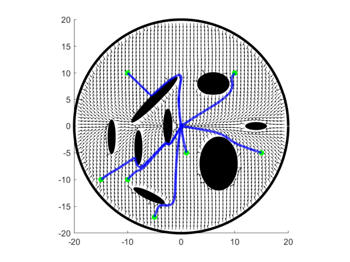(a)	(b)

Figure 3: (a)Trajectories generated by following the negative gradient of the RK Potential – that is $\dot{x}=g_{\textrm{nav}}$ – which is not a navigation function as condition (11) is violated. (b)Trajectories generated by following our proposed dynamics, that is $\dot{x}=g_{\textrm{new}}$. Trajectories which converge to a local minimum of $\varphi(x)$ end in a red square. We set $k=15$ and $x^{*}$ is the origin.

In this section, we compare the performance of our proposed dynamics $g_{\textrm{new}}$ to the performance of navigation function dynamics $g_{\textrm{nav}}$. We consider a discrete approximation for the flow $\dot{x}=g(x)$. In practice, the norm of the dynamics is generally very small. This may cause problems numerically when computing the direction as well as taking taking a long time for the agent to reach its target. Hence, what is often used in practice is to normalize the gradient by scaling it by a factor of $(\epsilon+\|g(x)\|)$, where $\epsilon>0$ (Whitcomb and Koditschek, 1991). As such the dynamics will be

$$x_{t+1}=x_{t}+\eta\frac{g(x_{t})}{\|g(x_{t})\|+\epsilon}$$ (44)

where $\eta$ is a constant step size. We set $\epsilon=10^{-4}$ and $\eta=0.01$ in (44) for all simulations.

First, we consider a world with eight ellipsoidal obstacles, and we compare the trajectories from several different initial positions. Then, we explore the effect of increasing the number of obstacles of randomly generated ellipsoidal worlds. The obstacles are generated such that condition (11) might fail. Therefore, increasing the number of obstacles results in fewer trajectories following $g_{\textrm{nav}}$ successfully reaching the target. In contrast, the corrected dynamics performs well even when the number of obstacles is large.

5.1 Correcting the Field

In this section, we show an ellipsoidal world with eight obstacles and several different initialization points. We designed the world such that condition (11) does not necessarily hold, thereby eliminating the guarantee that the Rimon Koditschek potential is a navigation function. The maximum to minimum ratio of the eigenvalues of the eight obstacles range between 2 and 50. The radius of the outer obstacle $\beta_{0}$ is equal to 20. The objective value of the function is chosen to be ${f_{0}}(x)=\|x\|^{2}$.

Figure 3 (a) shows the vector field and some trajectories for the navigation function dynamics $\dot{x}=g_{\textrm{nav}}$. Indeed, condition (11) is violated. As such, four of the trajectories converge to local minimum appearing behind the obstacles which violate the condition instead of to the target. We selected $k=15$ because this was the maximum value for $k$ considered in the analysis for worlds which violate the condition (Paternain et al., 2018).

We compare the trajectories of our proposed dynamics to the navigation function dynamics where the condition is violated. The Figure 3 (b) shows that with the same value of $k=15$, all of the trajectories converge to the target. The vector field plots show that there is only one stable point, the target located at the origin. This is consistent with Theorem 1.

5.2 Obstacles in ${\mathbb{R}}^{2}$

(a)	(b)

Figure 4: (a) Uncorrected Dynamics: Regardless of the value $k$, the ratio of successful simulations decreases as the number of obstacles increases. (b) Proposed Dynamics: By increasing $k$, the ratio of successful simulations remains high regardless of the number of obstacles

In this section, we explore the effect of increasing the number of obstacles on the percentage of successful trajectories. We define the external shell to be the a sphere with center $(0,0)$ and radius $r_{0}$. The center of each ellipsoid is drawn uniformly from $[-r_{0}/2,r_{0}/2]^{2}$. The maximum semiaxis $r_{i}$ is drawn uniformly from $[r_{0}/10,r_{0}/5]$. The positive definite matrices $A_{i}$ have eigenvalues $1$ and $\mu_{i}$, where $\mu_{i}$ is drawn randomly from $[1,r_{0}/2]$. The obstacles are then rotated by $\theta_{i}$ where $\theta_{i}$ is drawn randomly from $[-\pi/2,\pi/2]$. The obstacles are redrawn if they overlap. For the objective function, we consider a quadratic cost given by

$${f_{0}}(x)=(x-x^{*})^{\top}Q(x-x^{*}).$$ (45)

where $Q\in{\mathcal{M}}^{2\times 2}$ is a diagonal matrix with eigenvalues $\text{eig}(Q)=\{1,\lambda\}$ where $\lambda$ is drawn from $[0,r_{0}]$. The minimizer of the objective function $x^{*}$ is drawn uniformly from $[-r_{0}/2,r_{0}/2]^{2}$. The minimizer $x^{*}$ is redrawn if it is not in the free space. Finally, the initial position is drawn uniformly from $[-r_{0},r_{0}]^{2}$ and is redrawn if it is not in the interior of the free space. For our experiments, we set $r_{0}=20$. We then vary number of obstacles $m$ from two to seven. For tuning parameters $k=\{20,40,60\}$ we run 100 simulations for each $m\in\{2,\dots,7\}$. Each simulation is terminated successfully when the norm of the difference of $x_{t}$ and $x^{*}$ is less than the step size $\eta=0.01$. A simulation is terminated unsuccessfully if the agent collides with an obstacle - including the outer boundary - or the number of steps reaches $5\times 10^{4}$.

Figure 4 (a) shows the the results of the simulation for the uncorrected dynamics. For all values of $k$, the ratio of successful trajectories decreases as the number of obstacles increases. This is due to the fact that the increased number of obstacles increases the probability that there an obstacle violates condition (11). In contrast, Figures 4 (b) shows that as $k$ increases the ratio of successful trials increases. For $k=40$, the success percentage is always above $85\%$. For $k=60$, the success percentage is always above $95\%$.

The poor performance of $k=20$ in the corrected dynamics is due to the fact that we do not consider the outer obstacle $\beta_{0}$ in the dynamics – see Section 1. Because $g_{\textrm{nav}}$ includes $\beta_{0}$ as part of the dynamics, the agent is repelled away from the boundary thereby avoiding collision. In contrast, the correction dynamics avoid this collision by assuming that $k$ is large enough such that the agent is always moving inward when it is close to the outer boundary. As expected, the performance improves significantly with larger values of $k$.

6 Conclusions

We considered the problem of a point agent navigating to a target with a finite number of ellipsoidal obstacles of arbitrary eccentricity. In particular, we directly proposed dynamics which guarantee asymptotic convergence to the target from almost every initial condition given mild conditions on the target. We corroborated our theoretical results with numerical simulations on worlds in $\mathbb{R}^{2}$.

There are a number of possible extensions to this work. Apart from the generalizations to the case of disc robots, nonstationary obstacles, multiple agents, and online tuning of the parameter $k$, the ellipsoidal condition itself may be lifted. Given that the exact form of our proposed dynamics relies on estimating the distance and direction to both the target and obstacle, this approach may be used to extend convergence guarantees to not only convex obstacles, but non convex star obstacles as well. In fact, the explicit ellipsoidal form of the obstacles was used in the calculation of the Jacobian of the dynamics evaluated at a critical point only. Therefore, these results can be extended to convex obstacles by considering a general version of these proofs on the gradients of the obstacle-defining functions instead of the $x-x_{i}$ term.

In a related work, we have shown empirically that the same approach can be used for star obstacles (Kumar et al., 2020). Extending the convergence results to the case of star obstacles requires generalizing the proof of Theorem 1. Specifically, Lemmas 4.3 and 4.7 no longer hold due to the lack of separating hyperplanes between star obstacles. Borders between adjacent cells are not necessarily hyperplanes. Instead, Corrolary 4.5 would need to be used to describe a finite number of transitions between the two adjacent cells. This immediately breaks the directed acyclic graph on the obstacles. Instead, obstacles should be considered in pairs where the hyperplane does not exist between them, similar to the procedure described in Remark 1. Such a direction would close the gap between navigation with global information by allowing star worlds to be navigated without the need of a diffeomorphism.

Appendix A Proof of Lemma 4.9

We have

$$\dot{V}={(x-x^{*})}^{\top}\dot{x}.$$ (46)

Substituting (15) for $\dot{x}$,

$$\dot{V}=-\beta\|x-x^{*}\|^{2}-\frac{{f_{0}}}{k}\sum_{j=1}^{m}\bar{\beta}_{j}(x-x^{*})^{\top}(x-x_{j}).$$ (47)

First consider the set $\mathcal{F}_{>\varepsilon}\setminus N_{\varepsilon}(x^{*})$. Since we are bounded away from $x-x^{*}$, we can factor it out of (47). Invoking the bounds of (7) and (36), it holds that $\dot{V}<0$ when $K>B\lambda_{\varepsilon}m/2$. Next, consider evaluating $\dot{V}$ on $S_{i}\cup N_{\varepsilon}({\mathcal{O}}_{i})$ for any $i$. Split the summation term of (47) into

$$\begin{split}\dot{V}&=-\beta\|x-x^{*}\|^{2}+\frac{{f_{0}}}{k}\bar{\beta}_{i}(x-x^{*})^{\top}(x-x_{i})\\ &+\frac{{f_{0}}}{k}\sum_{j\neq i}\bar{\beta}_{j}(x-x^{*})^{\top}(x-x_{j})\\ &\leq-\beta\|x-x^{*}\|^{2}+\frac{{f_{0}}}{k}\bar{\beta}_{i}\|x-x^{*}\|\cdot\|x-x_{i}\|\\ &+\frac{{f_{0}}}{k}\sum_{j\neq i}\bar{\beta}_{j}(x-x^{*})^{\top}(x-x_{j})\\ \end{split},$$ (48)

where the inequality comes from applying Cauchy Schwartz. It holds that for $K>B\lambda_{\varepsilon}(m-1)/2-\beta_{i}^{-1}\|x-x^{*}\|\cdot\|x-x_{i}\|$, $\dot{V}<0$. This is trivially satisfied when $K>B\lambda_{\varepsilon}m/2$, as established earlier.

Finally, consider $N_{\varepsilon}(x^{*})$. By Cauchy Schwartz and the bounds (6) and (7), we bound

$$\dot{V}\leq-\beta\|x-x^{*}\|^{2}+\frac{\|x-x^{*}\|^{3}}{2k}mB\Lambda_{0}.$$ (49)

$\dot{V}$ is negative when $\|x-x^{*}\|<\lambda_{\varepsilon}m^{-1}B^{-1}\Lambda_{0}^{-1}$. This concludes the proof.

Appendix B Proof of Lemma 4.13

Evaluate

$$\dot{V}_{i}=$$

$$\frac{(x_{i}-x^{*})^{\top}\dot{x}}{\|x-x_{i}\|\cdot\|x_{i}-x^{*}\|}-\frac{(x-x_{i})^{\top}(x_{i}-x^{*})(x-x_{i})^{\top}\dot{x}}{\|x-x_{i}\|^{3}\cdot\|x_{i}-x^{*}\|}$$

Because $x,x^{*}\in\mathcal{F}$ and $x_{i}\notin\mathcal{F}$, $\|x-x_{i}\|\cdot\|x_{i}-x^{*}\|$ and $\beta_{j}$ for all $j$ are strictly positive. Replace $\dot{x}$ with (15) to obtain

$$\dot{V}_{i}=$$

$$\frac{\beta}{\|x-x_{i}\|\cdot\|x_{i}-x^{*}\|}\Bigg(-(x_{i}-x^{*})^{\top}(x-x^{*})$$

$$+\frac{(x-x_{i})^{\top}(x_{i}-x^{*})(x-x_{i})^{\top}(x-x^{*})}{\|x-x_{i}\|^{2}}$$

$$+\frac{{f_{0}}}{k}\sum_{j=1}^{m}\frac{1}{\beta_{j}}\bigg((x_{i}-x^{*})^{\top}(x-x_{j})$$

$$-\frac{(x-x_{i})^{\top}(x_{i}-x^{*})(x-x_{i})^{\top}(x-x_{j})}{\|x-x_{i}\|^{2}}\bigg)\Bigg)$$

Using the fact that $x-x^{*}=(x-x^{i})+(x_{i}-x^{*})$ and the decomposition (37), the first two terms are strictly negative. Namely, we obtain the bound

$$-\frac{\|x_{i}-x^{*}\|^{2}\cdot\|{\mathbf{p}}\|^{2}}{a^{2}\|x_{i}-x^{*}\|^{2}+\|{\mathbf{p}}\|^{2}}\leq-\frac{B\delta_{\perp}^{2}}{a^{2}B+\delta_{\perp}^{2}}<0,$$ (50)

where $B$ comes from (6), and we can invoke $\|\textbf{p}\|\geq\delta_{\perp}$ by the fact that we are in ${\mathcal{C}}_{i}\backslash{\mathcal{P}}_{i}$. The terms in the summation where $j=i$ cancel each other out. The summation terms can be upper bounded by invoking (6), (7) (41), (42), namely

$${f_{0}}\sum_{j\neq i}\big(\cdot\big)\leq 2P_{0}\lambda_{i,\perp}B\cdot\left(1+\frac{1}{\theta_{i}}\right).$$ (51)

Selecting

$$K_{i}^{\perp}:=2P_{0}\lambda_{i,\perp}\delta_{\perp}^{-2}\left(1+\frac{1}{\theta_{i}}\right)\left(a^{2}B+\delta_{\perp}^{2}\right)$$ (52)

completes the proof.

Appendix C Proof of Lemma 4.15

By $x\in N_{\varepsilon}({\mathcal{O}}_{i})$, we have that $\beta_{i}\leq\varepsilon$.

In the case of one obstacle, there is a critical point where

$$\beta_{i}(x-x^{*})=\frac{{f_{0}}}{k}(x-x_{i}).$$ (53)

This is when $x-x^{*}$ is aligned with $x-x_{i}$, when the obstacle is between the agent and the target. Let $x_{s}$ be the point where (53) holds. Then we can write for $a>1$

$$x_{s}-x^{*}=a(x_{s}-x_{i}).$$ (54)

This with (53) gives the following criterion for the critical point

$$\beta_{i}(x_{s})=\frac{{f_{0}}(x_{s})}{ak}.$$ (55)

To show that the point $x_{s}$ is an unstable equilibrium, consider the Jacobian of (15) $J(g_{\textrm{new}})$,

$$\begin{split}J(x_{s})&=-\beta I-\nabla\beta(x-x^{*})^{\top}\\ &+\frac{1}{k}\nabla\left({f_{0}}\bar{\beta}_{i}\right)(x-x_{i})^{\top}+\frac{1}{k}{f_{0}}\bar{\beta}_{i}I\\ &+\frac{1}{k}\beta_{i}J\left({f_{0}}\sum_{j\neq i}\prod_{\ell\neq j}\beta_{\ell}(x-x_{\ell})\right)\\ &+\frac{1}{k}\nabla\beta_{i}\left({f_{0}}\sum_{j\neq i}(x-x_{j})\right)^{\top}\end{split}$$ (56)

Define $\mathcal{E}$ to be the set of normal vectors that are orthogonal to $(x_{s}-x_{i})$

$$\mathcal{E}:=\left\{v\in\mathbb{R}^{n}\left|\|v\|=1,v^{\top}(x_{s}-x_{i})=0\right.\right\}.$$ (57)

The rank of $\mathcal{E}$ is $n-1$. Let $\left\{v_{1},\dots,v_{n-1}\right\}$ be a basis. Consider any $v_{i}$ and evaluate the Jacobian at $x_{s}$ where (53) holds,

$$\begin{split}v_{i}^{\top}&J(g_{\textrm{new}})v_{i}\big|_{x_{s}}=-\beta+\frac{1}{k}{f_{0}}\bar{\beta}_{i}\\ &+\frac{1}{k}v_{i}^{\top}\beta_{i}J\left({f_{0}}\sum_{j\neq i}\left(\prod_{\ell\neq j}\beta_{\ell}\right)(x-x_{j})\right)v_{i}\\ &=-\frac{\bar{\beta}_{i}{f_{0}}}{ak}+\frac{1}{k}{f_{0}}\bar{\beta}_{i}\\ &+\frac{1}{ak^{2}}v_{i}^{\top}J\left({f_{0}}^{2}\sum_{j\neq i}\left(\prod_{\ell\neq j}\beta_{\ell}\right)(x-x_{j})\right)v_{i}\end{split}$$ (58)

We because of (7) and (6), for any unit vector $n$, we can bound the final term as

$$\left\|n^{\top}J\left({f_{0}}^{2}\sum_{j\neq i}\prod_{\ell\neq j}\beta_{\ell}(x-x_{\ell})\right)n\right\|\leq C_{1}$$ (59)

Let $p_{0}:=\min_{x\notin C_{0}}{f_{0}}(x)$ and recall (20). As such, for

$$K_{{\mathbf{p}},i_{1}}=\frac{C_{1}}{p\varepsilon^{m-1}}\cdot\frac{a}{a-1},$$

with any $k>K_{{\mathbf{p}},i_{1}}$, we know that $v_{i}^{\top}J(x_{s})v_{i}$ is positive rendering that direction unstable.

Now consider the unit vector $w$ aligned with $(x_{s}-x_{i})$. In particular, we set $w=(x_{s}-x_{i})/\|x_{s}-x_{i}\|$. Consider evaluating $w^{\top}J(g_{\textrm{new}})w$ at $x_{s}$,

$$\begin{split}w^{\top}&J(g_{\textrm{new}})w\bigg|_{x_{s}}=-\beta-w^{\top}\nabla\beta(x-x^{*})^{\top}w+\frac{1}{k}{f_{0}}\bar{\beta}_{i}\\ &+\frac{1}{k}w^{\top}\nabla\left({f_{0}}\bar{\beta}_{i}\right)(x-x_{i})^{\top}w\\ &+\frac{\beta_{i}}{k}w^{\top}J\left({f_{0}}\sum_{j\neq i}\prod_{\ell\neq j}\beta_{\ell}\right)w\\ &+\frac{1}{k}w^{\top}\nabla\beta_{i}\left({f_{0}}\sum_{j\neq i}\left(\prod_{\ell\neq j}\beta_{\ell}\right)(x-x_{j})\right)w\end{split}$$ (60)

Split the second term using (14), and apply the relations (53) and (54) to obtain

$$\begin{split}w^{\top}&J(g_{\textrm{new}})w\bigg|_{x_{s}}=-a^{-1}\bar{\beta}_{i}\\ &+\frac{1}{k}\Bigg({f_{0}}\bar{\beta}_{i}\left(1-a^{-1}\right)\\ &-{f_{0}}a^{-1}w^{\top}\big(\sum_{j\neq i}\prod_{\ell\neq j}\beta_{\ell}\nabla\beta_{\ell}\big)(x-x^{*})^{\top}w\\ &+{f_{0}}a^{-1}\sum_{j\neq i}(x-x_{j})^{\top}w\\ &+w^{\top}\nabla({f_{0}}\bar{\beta}_{i})(x-x_{i})^{\top}w\Bigg)\\ &+\frac{1}{k^{2}}\Bigg({f_{0}}a^{-1}w^{\top}J\big({f_{0}}\sum_{j\neq i}\prod_{\ell\neq j}\beta_{\ell}(x-x_{j})\big)w\Bigg)\\ &\leq-\bar{\beta}_{i}a^{-1}+C_{2}k^{-1}+C_{3}k^{-2},\end{split}$$ (61)

where

$$\begin{split}&\Bigg\|{f_{0}}\bar{\beta}_{i}\left(1-a^{-1}\right)+{f_{0}}a^{-1}\sum_{j\neq i}(x-x_{j})^{\top}w\\ &-{f_{0}}a^{-1}w^{\top}\big(\sum_{j\neq i}\prod_{\ell\neq j}\beta_{\ell}\nabla\beta_{\ell}\big)(x-x^{*})^{\top}w\\ &+w^{\top}\nabla({f_{0}}\bar{\beta}_{i})(x-x_{i})^{\top}w\Bigg\|\leq C_{2},\end{split}$$ (62)

and

$$\Bigg\|{f_{0}}a^{-1}w^{\top}J\big({f_{0}}\sum_{j\neq i}\prod_{\ell\neq j}\beta_{\ell}(x-x_{j})\big)w\Bigg\|\leq C_{3}.$$ (63)

$C_{2}$ and $C_{3}$ are finite by (6) and (7). Then, for

$$K_{{\mathbf{p}},i_{2}}:=\max\left\{\frac{C_{2}\pm\sqrt{C_{1}^{2}+4C_{3}\bar{\beta}_{i}(x_{s,i})a^{-1}}}{a}\bar{\beta}_{i}(x_{s,i})\right\},$$

with any $k>K_{{\mathbf{p}},i_{2}}$, we know that $w^{\top}J(g_{\textrm{new}})w$ is negative. Choose $K_{{\mathbf{p}},i}=\max\{K_{{\mathbf{p}},i_{1}},K{{\mathbf{p}},i_{2}}\}$ to complete the proof.

References

- Arslan and Koditschek (2016) O. Arslan and D. E. Koditschek. Sensor-based reactive navigation in unknown convex sphere worlds. The International Journal of Robotics Research, page 0278364918796267, 2016.
- Bhattacharya et al. (2007) S. Bhattacharya, S. Candido, and S. Hutchinson. Motion strategies for surveillance. In Robotics: Science and Systems, 2007.
- Blanchini (1999) F. Blanchini. Set invariance in control. Automatica, 35(11):1747–1767, 1999.
- Boyd and Vandenberghe (2004) S. Boyd and L. Vandenberghe. Convex optimization. Cambridge university press, 2004.
- Dimarogonas and Johansson (2008) D. V. Dimarogonas and K. H. Johansson. Decentralized connectivity maintenance in mobile networks with bounded inputs. In 2008 IEEE International Conference on Robotics and Automation, pages 1507–1512. IEEE, 2008.
- Filippidis and Kyriakopoulos (2012) I. F. Filippidis and K. J. Kyriakopoulos. Navigation functions for everywhere partially sufficiently curved worlds. In Robotics and Automation (ICRA), 2012 IEEE International Conference on, pages 2115–2120. IEEE, 2012.
- Fitzgibbon et al. (1999) A. Fitzgibbon, M. Pilu, and R. B. Fisher. Direct least square fitting of ellipses. IEEE Transactions on pattern analysis and machine intelligence, 21(5):476–480, 1999.
- Ghaffarkhah and Mostofi (2009) A. Ghaffarkhah and Y. Mostofi. Communication-aware target tracking using navigation functions-centralized case. In 2009 Second International Conference on Robot Communication and Coordination, pages 1–8. IEEE, 2009.
- Hart et al. (1968) P. E. Hart, N. J. Nilsson, and B. Raphael. A formal basis for the heuristic determination of minimum cost paths. IEEE transactions on Systems Science and Cybernetics, 4(2):100–107, 1968.
- Koditschek and Rimon (1990) D. E. Koditschek and E. Rimon. Robot navigation functions on manifolds with boundary. Advances in applied mathematics, 11(4):412–442, 1990.
- Kumar et al. (2020) H. Kumar, S. Paternain, and A. Ribeiro. Navigation of a quadratic potential with star obstacles. In 2020 American Control Conference (ACC), pages 2043–2048. IEEE, 2020.
- LaValle (1998) S. M. LaValle. Rapidly-exploring random trees: A new tool for path planning. 1998.
- LaValle (2006) S. M. LaValle. Planning algorithms. Cambridge university press, 2006.
- Li and Griffiths (2004) Q. Li and J. G. Griffiths. Least squares ellipsoid specific fitting. In null, page 335. IEEE, 2004.
- Lionis et al. (2008) G. Lionis, X. Papageorgiou, and K. J. Kyriakopoulos. Towards locally computable polynomial navigation functions for convex obstacle workspaces. In Robotics and Automation, 2008. ICRA 2008. IEEE International Conference on, pages 3725–3730. IEEE, 2008.
- Loizou (2011) S. G. Loizou. The navigation transformation: Point worlds, time abstractions and towards tuning-free navigation. In 2011 19th Mediterranean Conference on Control & Automation (MED), pages 303–308. IEEE, 2011.
- Loizou (2012) S. G. Loizou. Navigation functions in topologically complex 3-d workspaces. In 2012 American Control Conference (ACC), pages 4861–4866. IEEE, 2012.
- Loizou (2017) S. G. Loizou. The navigation transformation. IEEE Transactions on Robotics, 33(6):1516–1523, 2017.
- Murphy et al. (2008) R. R. Murphy, S. Tadokoro, D. Nardi, A. Jacoff, P. Fiorini, H. Choset, and A. M. Erkmen. Search and rescue robotics. In Springer handbook of robotics, pages 1151–1173. Springer, 2008.
- Paternain and Ribeiro (2019) S. Paternain and A. Ribeiro. Stochastic artificial potentials for online safe navigation. IEEE Transactions on Automatic Control, 65(5):1985–2000, 2019.
- Paternain et al. (2018) S. Paternain, D. E. Koditschek, and A. Ribeiro. Navigation functions for convex potentials in a space with convex obstacles. IEEE Transactions on Automatic Control, 63(9):2944–2959, 2018.
- Rimon and Koditschek (1991) E. Rimon and D. E. Koditschek. The construction of analytic diffeomorphisms for exact robot navigation on star worlds. Transactions of the American Mathematical Society, 327(1):71–116, 1991.
- Rimon and Koditschek (1992) E. Rimon and D. E. Koditschek. Exact robot navigation using artificial potential functions. IEEE Transactions on robotics and automation, 8(5):501–518, 1992.
- Tanner and Kumar (2005) H. G. Tanner and A. Kumar. Formation stabilization of multiple agents using decentralized navigation functions. In Robotics: Science and systems, volume 1, pages 49–56. Boston, 2005.
- Taylor and LaValle (2009) K. Taylor and S. M. LaValle. I-bug: An intensity-based bug algorithm. In Robotics and Automation, 2009. ICRA’09. IEEE International Conference on, pages 3981–3986. IEEE, 2009.
- Vasilopoulos et al. (2020) V. Vasilopoulos, G. Pavlakos, S. L. Bowman, J. D. Caporale, K. Daniilidis, G. J. Pappas, and D. E. Koditschek. Reactive semantic planning in unexplored semantic environments using deep perceptual feedback. IEEE Robotics and Automation Letters, 5(3):4455–4462, 2020.
- Vrohidis et al. (2018) C. Vrohidis, P. Vlantis, C. P. Bechlioulis, and K. J. Kyriakopoulos. Prescribed time scale robot navigation. IEEE Robotics and Automation Letters, 3(2):1191–1198, 2018.
- Whitcomb and Koditschek (1991) L. L. Whitcomb and D. E. Koditschek. Automatic assembly planning and control via potential functions. In Intelligent Robots and Systems’ 91.’Intelligence for Mechanical Systems, Proceedings IROS’91. IEEE/RSJ International Workshop on, pages 17–23. IEEE, 1991.