DUAL-GLOW: Conditional Flow-Based Generative Model for Modality Transfer

Abstract

Positron emission tomography (PET) imaging is an imaging modality for diagnosing a number of neurological diseases. In contrast to Magnetic Resonance Imaging (MRI), PET is costly and involves injecting a radioactive substance into the patient. Motivated by developments in modality transfer in vision, we study the generation of certain types of PET images from MRI data. We derive new flow-based generative models which we show perform well in this small sample size regime (much smaller than dataset sizes available in standard vision tasks). Our formulation, DUAL-GLOW, is based on two invertible networks and a relation network that maps the latent spaces to each other. We discuss how given the prior distribution, learning the conditional distribution of PET given the MRI image reduces to obtaining the conditional distribution between the two latent codes w.r.t. the two image types. We also extend our framework to leverage “side” information (or attributes) when available. By controlling the PET generation through “conditioning” on age, our model is also able to capture brain FDG-PET (hypometabolism) changes, as a function of age. We present experiments on the Alzheimer’s Disease Neuroimaging Initiative (ADNI) dataset with 826 subjects, and obtain good performance in PET image synthesis, qualitatively and quantitatively better than recent works.

1 Introduction

Figure 1: The DUAL-GLOW framework. For the conditional module, the dashed and dotted pieces are added and removed respectively. The colored circle represents the latent code whereas the gray one is the image or the intermediate output.

Positron Emission Tomography (PET) images provide a three-dimensional image volume reflecting metabolic activity in the tissues, e.g., brain regions, which is a key imaging modality for a number of diseases (e.g., Dementia, Epilepsy, Head and Neck Cancer). Compared with Magnetic Resonance (MR) imaging, the typical PET imaging procedure usually involves radiotracer injection and a high cost associated with specialized hardware and tools, logistics, and expertise. Due to these factors, Magnetic Resonance (MR) imaging is much more ubiquitous than PET imaging in both clinical and research settings. Clinically, PET imaging is often only considered much further down the pipeline, after information from other non-invasive approaches has been collected. It is not uncommon for many research studies to include MR images for all subjects, and acquire specialized PET images only for a smaller subset of participants.

Other use cases. Leaving aside the issue of disparity in costs between MR and PET, it is not uncommon to find that due to a variety of reasons other than cost, a (small or large) subset of individuals in a study have one or more image scans unavailable. Finding ways to “generate” one type of imaging modality given another is attracting a fair bit of interest in the community and a number of ideas have been presented [34]. Such a strategy, if effective, can increase the sample sizes available for statistical analysis and possibly, even for training downstream learning models for diagnosis.

Related Work. Modality transfer can be thought of “style transfer” [16, 49, 50, 19, 42, 31, 24, 6, 25, 15, 22, 11, 30, 27, 43] in the context of medical images and a number of interesting results in this area have appeared [23, 17, 44, 32, 28, 13, 34]. Existing methods, mostly based on deep learning for modality transfer, can be roughly divided into two categories: Auto-encoders and Generative Adversarial Networks (GANs) [12, 18, 3]. Recall that auto-encoders are composed of two modules, encoder and decoder. The encoder maps the input to a hidden code $h$, and the decoder maps the hidden code to the output. The model is trained by minimizing the loss in the output Euclidean space with standard norms ($\ell_{1}$, $\ell_{2}$). A U-Net structure, introduced in [36], is typically used for leveraging local and hierarchical information to achieve an accurate reconstruction. Although the structure in auto-encoders is elegant with reasonable efficiency and a number of authors have reported good performance [32, 37], constructions based on minimizing the $\ell_{2}$ loss often produce blurry outputs, as has been observed in [34]. Partly due to these reasons, more recent works have investigated other generative models. Recently, one of the prominent generative models in use today, GANs [12], has seen much success in natural image synthesis [3], estimating the generative model via an adversarial process. Despite their success in generating sharp realistic images, GANs usually suffer from “mode collapse”, that tends to produce limited sample variety [4, 1]. This issue is only compounded in medical images, where the maximal mode may simply be attributed to anatomical structure shared by most subjects. Further, sample sizes are often much smaller in medical imaging compared to computer vision, which necessitates additional adjustments to the architecture and parameters, as we found in our experiments as well.

Flow-based generative models. Another family of methods, flow-based generative models [7, 8, 21], has been proposed for variational inference and natural image generation and have only recently begun to gain attention in the computer vision community. A (normalizing) flow, proposed in [35], uses a sequence of invertible mappings to build the transformation of a probability density to approximate a posterior distribution. The flow starts with an initial variable and maps it to a variable with a simple distribution (e.g., isotropic Gaussian) by repeatedly applying the change of variable rule, similar to the inference procedure in an encoder network. For the image generation task, the initial variable is the real image with some unknown probability function. Designating a well-designed inference network, the flow will learn an accurate mapping after training. Because the flow-based model is invertible, the generation of synthetic images is straightforward by sampling from the simple distribution and “flowing” through the map in reverse. Compared with other generative models and Autoregressive Models [33], flow-based methods allow tractable and accurate log-likelihood evaluation during the training process, while also providing an efficient and exact sampling from the simple prior distribution at test time.

Where is the gap? While flow-based generative models have been successful in image synthesis, it is challenging to leverage them directly for modality transfer. It is difficult to apply existing flow-based methods to our task due to the invertibility constraint in the inference network. Apart from various technical issues, consider an intuitive example. Given an MRI, we should expect that there would be many solutions of corresponding PET images, and vice versa. Ideally, we prefer the model to provide a conditional distribution of the PET given an MRI – such a conditional distribution can also be meaningfully used when additional information about the subject is available.

This work. Motivated by the above considerations, we propose a novel flow-based generative model, DUAL-GLOW, for MRI-to-PET image generation. The value of our model includes explicit latent variable representations, exact and efficient latent-variable inference, and the potential for memory and computation savings through constant network size. Utilizing recent developments in flow-based generative models by [21], DUAL-GLOW is composed of two invertible inference networks and a relation CNN network, as pictured in Figure 1. We adopt the multi-scale architecture with spliting technique in [8], which can significantly reduce the computational cost and memory. The two inference networks are built to project MRI and PET into two semantically meaningful latent spaces, respectively. The relation network is constructed to estimate the conditional distribution between paired latent codes. The foregoing properties of the DUAL-GLOW framework enable specific improvements in modality transfer from MRI to PET images. Sampling efficiency allows us to process and generate full 3D brain volumes.

Conditioning based on additional information. While the direct generation of PET from MRI has much practical utility, it is often also the case that a single MRI could correspond to a very different PET image – and which images are far more likely can be resolved based on additional information, such as age or disease status. However, a challenge arises due to the high correlation between the input MR image and side information: traditional conditional frameworks [29, 21] cannot effectively generate meaningful images in this setting. To accurately account for this correlation, we propose a new conditional framework, see Figure 1, where two small discriminators (Multiple Layer Perceptron, MLP) are concatenated at the end of the top inference networks to faithfully extract the side information contained in the images. The remaining two discriminators concatenated at the left invertible inference network are combined with Gradient Reverse Layers (GRL), proposed in [10], to exclude the side information which exists in the latent codes except at the top-most layer. After training, sampling from the conditional distribution allows the generation of diverse and meaningful PET images. Extensive experiments show the efficiency of this exclusion architecture in the conditional framework for side information manipulation.

Contributions. This paper provides: (1) A novel flow-based generative model for modality transfer, DUAL-GLOW. (2) A complete end-to-end PET image generation from MRI for full three-dimensional volumes. (3) A simple extension that enables side condition manipulation – a practically useful property that allows assessing change as a function of age, disease status, or other covariates. (4) Extensive experimental analysis of the quality of PET images generated by DUAL-GLOW, indicating the potential for direct application in practice to help in the clinical evaluation of Alzheimer’s disease (AD).

2 Flow-based Generative Models

We first briefly review flow-based generative models to help motivate and present our algorithm. Flow based generative models, e.g., GLOW [21], typically deal with single image generation. At a high level, these approaches set up the task as calculating the log-likelihood of an input image with an unknown distribution. Because maximizing this log-likelihood is intractable, a flow is set up to project the data into a new space where it is easy to compute, as summarized below.

Let ${\bf x}$ be an image represented as a high-dimensional random vector in the image space with an unknown true distribution ${\bf x}\sim p^{\ast}({\bf x})$. We collect an i.i.d. dataset $\mathcal{D}$ with samples $\{{\bf x}^{i}\}_{i=1}^{n}$ and choose a model class $p_{\theta}({\bf x})$ with parameters $\theta$. Our goal is to find parameters $\hat{\theta}$ that produces $p_{\hat{\theta}}({\bf x})$ to best approximate $p^{\ast}({\bf x})$. This is achieved through maximization of the log-likelihood:

$$\mathcal{L}(\mathcal{D})=\frac{1}{n}\sum_{i=1}^{n}\log p_{\theta}({\bf x}^{i}).$$ (1)

In typical flow-based generative models [7, 8, 21], the generative process for ${\bf x}$ is defined in the following way:

$${\bf z}\sim p_{\theta}({\bf z}),\quad{\bf x}=g_{\theta}({\bf z}),$$ (2)

where ${\bf z}$ is the latent variable and $p_{\theta}({\bf z})$ has a (typically simple) tractable density, such as a spherical multivariate Gaussian distribution: $p_{\theta}({\bf z})=\mathcal{N}({\bf z};0,{\bf I})$. The function $g_{\theta}(\cdot)$ may correspond to a rich function class, but is invertible such that given a sample ${\bf x}$, latent-variable inference is done by ${\bf z}=f_{\theta}({\bf x})={g_{\theta}}^{-1}({\bf x})$. For brevity, we will omit subscript $\theta$ from $f_{\theta}$ and $g_{\theta}$.

We focus on functions where $f$ is composed of a sequence of invertible transformations: $f=f_{k}\circ\cdots\circ f_{2}\circ f_{1}$, where the relationship between ${\bf x}$ and ${\bf z}$ can be written as:

$${\bf x}{\mathrel{\to}^{f_{1}}}{\bf h}_{1}{\mathrel{\to}^{f_{2}}}{\bf h}_{2}\cdot\cdot\cdot{\mathrel{\to}^{f_{k}}}{\bf z}.$$ (3)

Such a sequence of invertible transformations is also called a (normalizing) flow [35]. Under the change of variables rule through (2), the log probability density function of the model (1) given a sample ${\bf x}$ can be written as:

$$\log p_{\theta}({\bf x}) =\log p_{\theta}({\bf z})+\log|det(d{\bf z}/d{\bf x})|$$ (4)

$$=\log p_{\theta}({\bf z})+\sum_{i=1}^{k}\log|det(d{\bf h}_{i}/d{\bf h}_{i-1})|$$ (5)

where we define ${\bf h}_{0}={\bf x}$ and ${\bf h}_{k}={\bf z}$ for conciseness. The scalar value $\log|det(d{\bf h}_{i}/d{\bf h}_{i-1})|$ is the logarithm of the absolute value of the determinant of the Jacobian matrix $(d{\bf h}_{i}/d{\bf h}_{i-1})$, also called the log-determinant. While it may look difficult, this value can be simple to compute for certain choices of transformations, as previous explored in [7]. For the transformations $\{f_{i}\}_{i=1}^{k}$ which characterizes the flow, there are several typical settings that result in invertible functions, including actnorms, invertible $1\times 1$ convolutions, and affine coupling layers [21]. Here we use affine coupling layers, discussed in further detail shortly. For more, details regarding these mappings we refer the reader to existing literature on flow-based models, including GLOW [21].

Figure 2: DUAL-GLOW for image generation.

Figure 3: Spliting.

3 Deriving DUAL-GLOW

In this section, we present our DUAL-GLOW framework for inter-modality transfer. We first discuss the derivation of the conditional distribution of a PET image given an MR image and then provide strategies for efficient calculation of its log-likelihood. Then, we introduce the construction of the invertible flow and show the calculation for the Jacobian matrix. Next, we build the hierarchical architecture for our DUAL-GLOW framework, which greatly reduces the computational cost compared to a flat structure. Finally, the conditional structure for side information manipulation is derived with additional discriminators.

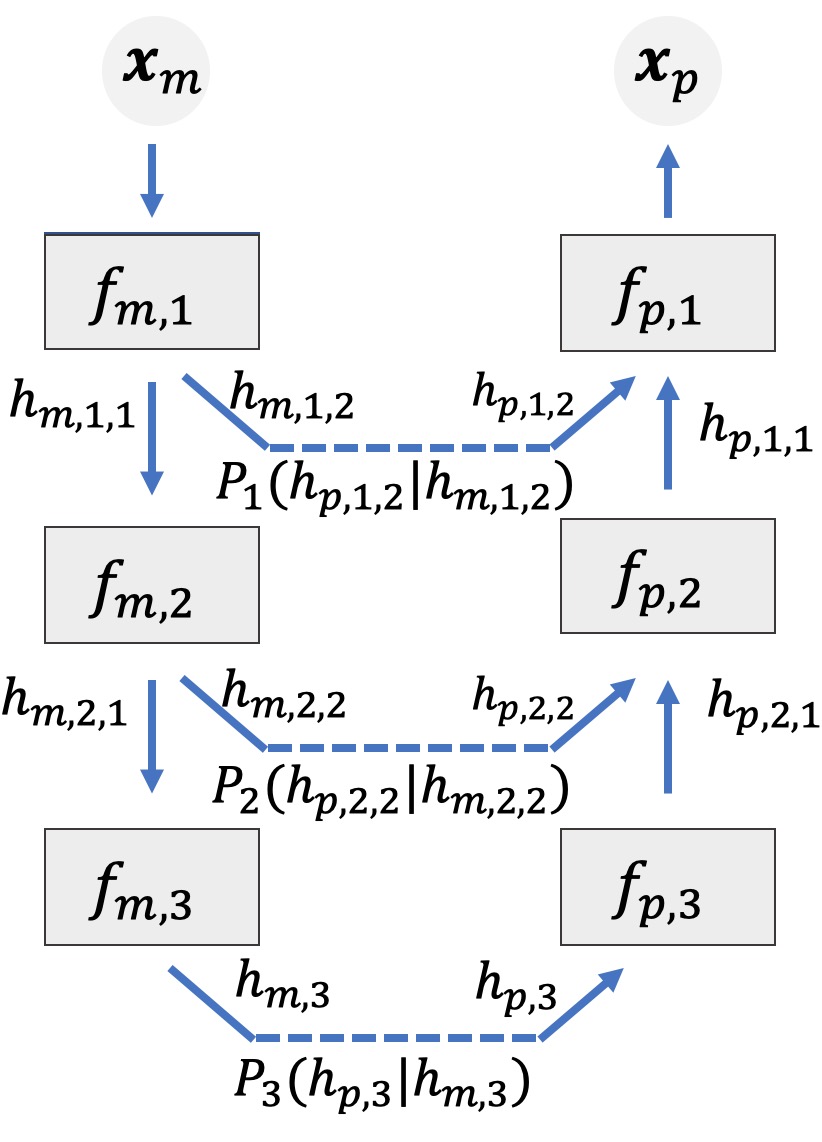
Log-Likelihood of the conditional Distribution. Let the data corresponding to the MR and PET images be denoted as $\mathcal{D}_{m}$ and $\mathcal{D}_{p}$. From a dataset $\mathcal{D}_{m}=\{{\bf x}_{m}^{i}\}_{i=1}^{n}$, we are interested in generating images which have the same properties as images in the dataset $\mathcal{D}_{p}=\{{\bf x}_{p}^{i}\}_{i=1}^{n}$. In our DUAL-GLOW model, we assume that there exists a flow-based invertible function $f_{p}$ which maps the PET image ${\bf x}_{p}$ to ${\bf z}_{p}=f_{p}({\bf x}_{p})$ and a flow-based invertible function $f_{m}$ which maps the MR image ${\bf x}_{m}$ to ${\bf z}_{m}=f_{m}({\bf x}_{m})$. The latent variables ${\bf z}_{p}$ and ${\bf z}_{m}$ help set up a conditional probability $p_{\theta}({\bf z}_{p}|{\bf z}_{m})$, given by

$$p_{\theta}({\bf z}_{p}|{\bf z}_{m})=\mathcal{N}({\bf z}_{p};\mu_{\theta}({\bf z}_{m}),\sigma_{\theta}({\bf z}_{m}))$$ (6)

The full mapping composed of $f_{p}$, $f_{m}$, $\mu_{\theta}$ and $\sigma_{\theta}$ formulates our DUAL-GLOW framework:

$${\bf x}_{m}{\mathrel{\to}^{f_{m}}}{\bf z}_{m}\xrightarrow{\mu_{\theta},\sigma_{\theta}}{\bf z}_{p}{\mathrel{\to}^{{f_{p}}^{-1}}}{\bf x}_{p},$$ (7)

see Figure 2. The invertible functions $f_{p}$ and $f_{m}$ are designed as flow-based invertible functions. The mean function $\mu_{\theta}$ and the covariance function $\sigma_{\theta}$ for $p_{\theta}({\bf z}_{p}|{\bf z}_{m})$ are assumed to be specified by neural networks. In this generating process, our goal is to maximize the log conditional probability $p_{\theta}({\bf x}_{p}|{\bf x}_{m})$. By the change of variable rule, we have that

$$\log p_{\theta}({\bf x}_{p}|{\bf x}_{m})=\log\left(p_{\theta}({\bf x}_{p},{\bf x}_{m})/p_{\theta}({\bf x}_{m})\right)$$ (8)

$$=\log p_{\theta}({\bf z}_{p}|{\bf z}_{m})+\log\left(\frac{|det(d({\bf z}_{p},{\bf z}_{m})/d({\bf x}_{p},{\bf x}_{m}))|}{|det(d{\bf z}_{m}/d{\bf x}_{m})|}\right)$$ (9)

$$=\log p_{\theta}({\bf z}_{p}|{\bf z}_{m})+\log\left(|det(d{\bf z}_{p}/d{\bf x}_{p})|\right).$$ (10)

Note that the Jacobian $d({\bf z}_{p},{\bf z}_{m})/d({\bf x}_{p},{\bf x}_{m})$ in (9) is, in fact, a block matrix

$$\frac{d({\bf z}_{p},{\bf z}_{m})}{d({\bf x}_{p},{\bf x}_{m})}=\left[\begin{array}[]{cc}d{\bf z}_{p}/d{\bf x}_{p}&0\\ 0&d{\bf z}_{m}/d{\bf x}_{m}\end{array}\right].$$ (11)

Recall that calculating the deteriminant of such a matrix is straightforward (see [38]), which leads directly to (10).

Without any regularization, maximizing such a conditional probability can make the optimization hard. Therefore, we may add a regularizer by controlling the marginal distribution $p_{\theta}({\bf z}_{m})$, which leads to our objective function

$$\max_{f_{m},f_{p},\mu_{\theta},\sigma_{\theta}} \log p_{\theta}({\bf z}_{p}|{\bf z}_{m})+\log(|det(\frac{d{\bf z}_{p}}{d{\bf x}_{p}})|)+\lambda\log p_{\theta}({\bf x}_{m})$$

$$=\log p_{\theta}({f_{p}}({\bf x}_{p})|f_{m}({\bf x}_{m}))+\log(|det(\frac{d{\bf z}_{p}}{d{\bf x}_{p}})|)$$

$$\quad+\lambda\log(p_{\theta}(f_{m}({\bf x}_{m}))|det(\frac{d{\bf z}_{m}}{d{\bf x}_{m}})|),$$ (12)

where $\lambda$ is a hyperparameter, $p_{\theta}({\bf z}_{m})=\mathcal{N}({\bf z}_{m};0,{\bf I})$ and $p_{\theta}({\bf z}_{p}|{\bf z}_{m})=\mathcal{N}({\bf z}_{p};\mu_{\theta}({\bf z}_{m}),\sigma_{\theta}({\bf z}_{m}))$.

Interestingly, compared to GLOW, our model does not introduce much additional complexity in computation. Let us see why. First, the marginal distribution $p_{\theta}({\bf z})$ in GLOW is replaced by $p_{\theta}({\bf z}_{p}|{\bf z}_{m})$ and $p_{\theta}({\bf z}_{m})$, which still has a simple and tractable density. Second, instead of one flow-based invertible function in GLOW, our DUAL-GLOW has two flow-based invertible functions $f_{p}$, $f_{m}$. Those functions are setup in parallel based on (12), extending the model size by a constant factor.

Flow-based Invertible Functions. In our work, we use an affine coupling layer to design the flows for the invertible functions $f_{p}$ and $f_{m}$. Before proceeding to the details, we omit subscripts $p$ and $m$ to simplify notations in this subsection. The invertible function $f$ is composed of a sequence of transformations $f=f_{k}\circ\cdots\circ f_{2}\circ f_{1}$, as introduced in (3). In DUAL-GLOW, $\{f_{i}\}_{i=1}^{k}$ are designed by using the affine coupling layer [8] following these equations:

$$\bf{\displaystyle h}_{i}=f_{i}({\bf h}_{i-1})\Leftrightarrow$$ (13)

$$\begin{cases}{\bf h}_{i;1:d_{1}}={\bf h}_{i-1;1:d_{1}}\\ \begin{aligned} {\bf h}_{i;d_{1}+1:d_{1}+d_{2}}=&({\bf h}_{i-1;d_{1}+1:d_{1}+d_{2}}\odot\,\exp(\textrm{s}({\bf h}_{i-1;1:d_{1}}))\\ &+\;\;\textrm{t}({\bf h}_{i-1;1:d_{1}}),\end{aligned}\end{cases}$$

where $\,\odot\,$ denotes element-wise multiplication, ${\bf h}_{i}\in R^{d_{1}+d_{2}}$, ${\bf h}_{i;1:d_{1}}$ the first $d_{1}$ dimensions of ${\bf h}_{i}$, and ${\bf h}_{i;d_{1}+1:d_{1}+d_{2}}$ the remaining $d_{2}$ dimensions of ${\bf h}_{i}$. The functions $s(\cdot)$ and $t(\cdot)$ are nonlinear transformations where it makes sense to use deep convolutional neural networks (DCNNs). This construction makes the function $f$ invertible. To see this, we can easily write the inverse function ${f_{i}}^{-1}$ for $f_{i}$ as

$$\bf{\displaystyle h}_{i-1}=(f_{i})^{-1}({\bf h}_{i})\Leftrightarrow$$ (14)

$$\begin{cases}{\bf h}_{i-1;1:d_{1}}={\bf h}_{i;1:d_{1}}\\ \begin{aligned} {\bf h}_{i-1;d_{1}+1:d_{1}+d_{2}}=&({\bf h}_{i;d_{1}+1:d_{1}+d_{2}}-\textrm{t}({\bf h}_{i;1:d_{1}}))\\ &\;\odot\;\exp(-\textrm{s}({\bf h}_{i;1:d_{1}})).\end{aligned}\end{cases}$$

In addition to invertibility, this structure also tells us that the $\log(|det(d{\bf z}_{p}/d{\bf x}_{p})|)$ term in our objective (12) has a simple and tractable form. Computing the Jacobian, we have:

$$\frac{\partial f_{i}({\bf h}_{i-1})}{\partial{\bf h}_{i-1}}=\left[\begin{array}[]{cc}\textrm{I}_{1:d_{1}}&0\\ \frac{\partial f_{i;d_{1}+1:d_{1}+d_{2}}}{\partial{\bf h}_{i-1;1:d_{1}}}&\;\;\textrm{diag}\big(\exp\big(\textrm{s}({\bf h}_{i-1;1:d_{1}})\big)\big)\end{array}\right],$$ (15)

where $I_{1:d_{1}}\in R^{d_{1}\times d_{1}}$ is an identity matrix. Therefore,

$$\log(|det(d{\bf z}_{p} /d{\bf x}_{p})|)=\sum_{i=1}^{k}\log(|det(d{\bf h}_{i}/d{\bf h}_{i-1})|)$$

$$=\sum_{i=1}^{k}\log(|det(\textrm{diag}\big(\exp\big(\textrm{s}({\bf h}_{i-1;1:d_{1}})\big)\big))|)$$

$$=\sum_{i=1}^{k}\log\left|\exp\left(\sum_{j=1}^{d_{1}}\textrm{s}({\bf h}_{i-1;j})\right)\right|$$

which can be computed easily and efficiently, requiring no on-the-fly matrix inversions [21].

Efficiency from Hierarchical Structure. The flow $f=f_{k}\circ\cdots f_{2}\circ f_{1}$ can be viewed as a hierarchical structure. For the two datasets $\mathcal{D}_{m}=\{{\bf x}_{m}^{i}\}_{i=1}^{n}$ and $\mathcal{D}_{p}=\{{\bf x}_{p}^{i}\}_{i=1}^{n}$, it is computationally expensive to make all features of all samples go through the entire flow. Following implementation strategies in previous flow-based models, we use the splitting technique to speed up DUAL-GLOW in practice, see Figure 3. When a sample ${\bf x}$ reaches the $i$-th transformation $f_{i}$ in the flow as ${\bf h}_{i-1}$, we split ${\bf h}_{i-1}$ in two parts ${\bf h}_{i-1,1}$ and ${\bf h}_{i-1,2}$, and take only one part ${\bf h}_{i-1,1}$ through $f_{i}$ to become ${\bf h}_{i}=f_{i}({\bf h}_{i-1,1})$. The other part ${\bf h}_{i-1,2}$ is taken out from the flow without further transformation. Finally, all those split parts $\{{\bf h}_{i,2}\}_{i=1}^{k-1}$ and the top-most ${\bf h}_{k}$ are concatenated together to form ${\bf z}$. By using this splitting technique in the flow hierarchy, the part leaving the flow “early” goes through fewer transformations. As discussed in GLOW and previous flow-based models, each transformation $f_{i}$ is usually rich enough that splitting saves computation without losing much quality in practice. We provide the computational complexity in the appendix. Additionally, this hierarchical representation enables a more succinct extension to allow side information manipulation.

How to condition based on side information? As stated above, additional covariates should influence the PET image we generate, even with a very similar MRI. A key assumption in many conditional side information frameworks is that these two inputs (the input MR and the covariate) are independent of each other. Clearly, however, there exists a high correlation between MRI and side information such as age or gender or disease status. In order to effectively incorporate this into our model, it is necessary to disentangle the side information from the intrinsic properties encoded in the latent representation ${\bf z}_{m}$ of the MR image.

Let $c$ denote the side information, typically a high-level semantic label (age, sex, disease status, genotype). In this case, we expect that the effect of this side information would be at a high level in relation to individual image voxels. As such, we expect that only the highest level of DUAL-GLOW should be affected by this. The latent variables ${\bf z}_{p}$ should be conditioned on side variable $c$ and ${\bf z}_{m}=\{{\bf h}_{i,2}\}_{i=1}^{k}$ except ${\bf h}_{k}$. Thus, we can rewrite the conditional probability in (12) by adding $c$:

$$\max_{f_{m},f_{p},\mu_{\theta},\sigma_{\theta}} \log p_{\theta}({\bf z}_{p}|{\bf z}^{\prime}_{m},c)$$ (16)

$$+\log(|det(\frac{d{\bf z}_{p}}{d{\bf x}_{p}})|)+\lambda\log p_{\theta}({\bf x}_{m}),$$

where ${\bf z}^{\prime}_{m}=\{{\bf h}_{i,2}\}_{i=1}^{k-1}$ is independent on $c$, and

$$p_{\theta}({\bf z}_{p}|{\bf z}^{\prime}_{m},c)=\mathcal{N}({\bf z}_{p};\mu_{\theta}({\bf z}^{\prime}_{m},c),\sigma_{\theta}({\bf z}^{\prime}_{m},c)).$$ (17)

To disentangle the latent representation ${\bf z}^{\prime}_{m}$ and exclude the side information in ${\bf z}^{\prime}_{m}$, we leverage the well-designed conditional framework composed of both flow and discriminators. Specifically, the condition framework tries to exclude the side information from $\{{\bf h}_{i,2}\}_{i=1}^{k-1}$ and keep it in ${\bf h}_{k}$ at the top level during training time. To achieve this, we concatenate a simple discriminator for each $\{f_{i}\}_{i=1}^{k-1}$ and add a Gradient Reversal Layer (GRL), introduced in [10], at the beginning of the network. These classifiers are used for distinguishing the side information in a supervised way. The GRL acts as the identity function during the forward-propagation and reverses the gradient in back-propagation. Therefore, minimizing the classification loss in these classifiers is equivalent to pushing the model to exclude the information gained by this side information, leading to the exclusive representation ${\bf z}^{\prime}_{m}=\{{\bf h}_{i,2}\}_{i=1}^{k-1}$. We also add a classifier without GRL at the top level of $f_{m},f_{p}$ that explicitly preserves this side information at the highest level.

Finally, the objective is the log-likelihood loss in (16) plus the classification losses, which can be jointly optimized by the popular optimizer AdaMax [20]. The gradient is calculated in a memory efficient way inspired by [5]. After training the conditional framework, we achieve PET image generation influenced both by MRI and side information.

4 Experiments

Figure 4: Box plot of MAE metrics for different methods.

MRI GroundTruth Synthetic

MRI GroundTruth Synthetic

MRI GroundTruth Synthetic

Figure 5: Synthetic images are meaningful for subjects in both extremes of disease spectrum. Left: CN. Middle: MCI. Right: AD. The generated PET images show consistency of hypometabolism (less red, more yellow) with the ground truth image. (Best viewed in color; montages shown in the appendix).

We evaluate the model’s efficacy on the ADNI dataset both against ground truth images and for downstream applications. We conduct extensive quantitative experiments which show that DUAL-GLOW outperforms the baseline method consistently. Our generated PET images show desirable clinically meaningful properties which is relevant for their potential use in Alzheimer’s Disease diagnosis. The conditional framework also shows promise in tracking hypometabolism as a function of age.

4.1 ADNI Dataset

Data. The Alzheimer’s Disease Neuroimaging Initiative (ADNI) provides a large database of studies directly aimed at understanding the development and pathology of Alzheimer’s Disease. Subjects are diagnosed as cognitively normal (CN), significant memory concern (SMC), early mild cognitive impairment (EMCI), mild cognitive impairment (MCI), late mild cognitive impairment (LMCI) or having Alzheimer’s Disease (AD). FDG-PET and T1-weighted MRIs were obtained from ADNI, and pairs were constructed by matching images with the same subject ID and similar acquisition dates.

Preprocessing. Images were processed using SPM12 [2]. First, PET images were aligned to the paired MRI using coregistration. Next, MR images were nonlinearly mapped to the MNI152 template. Finally, PET images were mapped to the standard MNI space using the same forward warping identified in the MR segmentation step. Voxel size was fixed for all volumes to $1.5\times 1.5\times 1.5\>mm^{3}$, and the final volume size obtained for both MR and PET images was $64\times 96\times 64$. Through this workflow, we finally obtain 806 MRI/PET clean pairs. The demographics of the dataset are provided in the appendix. In the following experiments, we randomly select 726 subjects as the training data and the remaining 80 as testing within a 10-fold evaluation scheme.

Framework Details. The DUAL-GLOW architecture outlined above was trained using Nvidia V100 GPUs with Tensorflow. There are $4$ “levels” in our invertible network, each containing $16$ affine coupling layers. The nonlinear operators $\textrm{s}(\cdot)$ and $\textrm{t}(\cdot)$ are small networks with three 3D convolutional layers. For the hierarchical correction learning network, we split the hidden codes of the output of the first three modules in the invertible network and design four 3D convolutional networks for all latent codes. For the conditional framework case, we concatenate the five discriminators to the tail of all four levels of the MRI inference network and the top-most level of the PET inference network. The GRL is added between the inference network and the first three discriminators. The hyperparameter $\lambda$ is the regularizer and set to $0.001$. For all classification losses, we set the weight to $0.01$. The model was trained using the AdamMax optimizer with an initial learning rate set to $0.001$ and exponential decay rates $0.9$ for the moment estimates. We train the model for $90$ epochs. Our implementation is available at https://github.com/haolsun/dual-glow.

	MRI	50	60	70	80	90	100
AD
CN

Figure 6: Conditioning on age should yield generated images that show increased hypometabolism with age. These are representative results from our PET generation as a function of age. As we scan left to right, we indeed see a decrease in metabolism (less red, more yellow) which is completely consistent with what we would expect in aging. (Best viewed in color; montages shown in the appendix).

4.2 Generated versus Ground Truth consistency

We begin our model evaluation by comparing outputs from our model to 4 state-of-the-art methods used previously for similar image generation tasks, conditional GANs (cGANs) [32], cGANs with U-Net architecture (UcGAN) [36], Conditional VAE (C-VAE) [9, 39], pix2pix [16]. Additional experimental setup details are in the appendix. We compare using commonly-used quantitative measures computed over the held out testing data. These include Mean Absolute Error (MAE), Correlation Coefficients (CorCoef), Peak Signal-to-Noise Ratio (PSNR), and Structure Similarity Index (SSIM). For Cor_Coef, PSNR and SSIM, higher values indicate better generation of PET images. For MAE, the lower the value, the better is the generation. As seen in Table 1 and Figure 4, our model competes favorably against other methods.

Table 1: Quantitative comparison results on 10-fold cross-validation.

METHOD	cGAN	UcGAN	C-VAE	pix2pix	DUAL-GLOW
CorCoef	$0.956$	$0.963$	$\bm{0.980}$	$0.967$	$0.975$
PSNR	$27.37\pm 2.07$	$27.84\pm 1.23$	$28.69\pm 2.06$	$27.54\pm 1.95$	$\bm{29.56}\pm\bm{2.66}$
SSIM	$0.761\pm 0.08$	$0.780\pm 0.06$	$0.817\pm 0.06$	$0.783\pm 0.05$	$\bm{0.898}\pm\bm{0.06}$

Figure 9 shows test images generated after 90 epochs for Cognitively Normal and Alzheimer’s Disease individuals. Qualitatively, not only is the model able to accurately reconstruct large scale anatomical structures but it is also able to identify minute, sharp boundaries between gray matter and white matter. While here we focus on data from individuals with a clear progression of Alzheimer’s disease from those who are clearly cognitively healthy, in preclinical cohorts where disease signal may be weak, accurately constructing finer-grained details may be critical in identifying those who may be undergoing neurodegeneration due to dementia. More results are shown in the appendix.

4.3 Scientific Evaluation of Generation

As we saw above, our method is able to learn the modality mapping from MRI to PET. However, often image acquisition is used as a means to an end: typically towards disease diagnosis or informed preventative care. While the generated images may seem computationally and visually coherent, it is important that the images generated add some value towards these downstream analyses.

We also evaluate the generated PET images for disease prediction and classification. Using the AAL atlas, we obtain all 116 ROIs via atlas-based segmentation [45] and use the mean intensity of each as image features. A support vector machine (SVM) is trained with the standard RBF kernel (e.g., see [14]) to predict binary disease status (Normal, EMCI, SMC vs. MCI, LMCI, AD) for both the ground truth and the generated images. The SVM trained on generated images achieves comparable accuracy and false positive/negative rates (Table 2), suggesting that the generated images contain sufficient discriminative signal for disease diagnosis.

Table 2: Validation on the ground truth and synthetic images for the AD/CN classification.

	Ground Truth	Synthetic
Accuracy	$94\%$	$91\%$
False Negative Rate	$6\%$	$6\%$
False Positive Rate	$0\%$	$3\%$

Adjusting for Age with Conditioning. The conditional framework naturally allows us to evaluate potential developing pathology as an individual ages. Training the full conditional DUAL-GLOW model, we use ground truth “side” information (age) as the conditioning variable described above. Figure 13 shows the continuous change in the $3$ generated images given various age labels for the same MRI. The original image (left) is at age $50$, and as we increase age from $60$ to $100$, increased hypometabolism becomes clear. To quantitatively evaluate our conditional framework, we plot the mean intensity value of a few key ROIs. As we see in Figure 7, the mean intensity values show a downward trend with age, as expected. While there is a clear ‘shift’ between AD, MCI, and CN subjects (blue dots lie above red dots, etc.), the wide variance bands indicate a larger sample size may be necessary to derive statistically sound conclusions (e.g., regarding group differences). Additional results and details can be found in the appendix.

Figure 7: The mean intensity with 95% standard deviation bands of $3$ ROIs with the change of age for all test subjects. The clear downward trend reflects expected hypometabolism as a function of age.

4.4 Other Potential Applications

While not a key focus of our work, to show the model’s generality on visually familiar images we directly test DUAL-GLOW’s ability to generate images on a standard computer vision modality transfer task. Using the UT-Zap50K dataset [48, 47] of shoe images, we construct HED [46] edge images as “sketches”, similar to [16]. We aim to learn a mapping from sketch to shoe. We also create a cartoon face dataset based on CelebA [26] and train our model to generate a realistic image from the cartoon face. Fig. 8 shows the results of applying our model (and ground truth). Clearly, more specialized networks designed for such a task will yield more striking results, but these experiments suggest that the framework is general and applicable in additional settings. These results are available on the project homepage and in the appendix.

Input	Generated	Ground Truth

Figure 8: Sample generation using DUAL-GLOW. The first row: UT-Zap50K dataset. The second row: CartoonFace dataset.

5 Conclusions

We propose a flow-based generative model, DUAL-GLOW, for inter-modality transformation in medical imaging. The model allows for end-to-end PET image generation from MRI for full three-dimensional volumes, and takes advantage of explicitly characterizing the conditional distribution of one modality given the other. While inter-modality transfer has been reported using GANs, we present improved results along with the ability to condition the output easily. Applied to the ADNI dataset, we are able to generate sharp synthetic PET images that are scientifically meaningful. Standard correlation and classification analysis demonstrates the potential of generated PET in diagnosing Alzheimer’s Disease, and the conditional side information framework is promising for assessing the change of spatial metabolism with age.

Acknowledgments. HS was supported by Natural Science Foundation of China (Grant No. 61876098, 61573219) and scholarships from China Scholarship Council (CSC). Research was also supported in part by R01 AG040396, R01 EB022883, NSF CAREER award RI 1252725, UW Draper Technology Innovation Fund (TIF) award, UW CPCP AI117924 and a NIH predoctoral fellowship to RM via T32 LM012413.

6 Appendix

In this supplement, We provide extensive additional details regarding the neuroimaging experiments and some theoretical analysis.

6.1 The ADNI dataset

Data used in the experiments for this work were obtained directly from the Alzheimer’s Disease Neuroimaging Initiative (ADNI) database (adni.loni.usc.edu). As such, the investigators within the ADNI contributed to the design and implementation of ADNI and/or provided data but did not participate in analysis or writing of this report. A complete listing of ADNI investigators can be found at: http://adni.loni.usc.edu/wp-content/uploads/how_to_apply/ADNI_Acknowledgement_List.pdf. The ADNI was launched in 2003 as a public-private partnership, led by Principal Investigator Michael W. Weiner, MD. The primary goal of ADNI has been to test whether serial magnetic resonance imaging (MRI), positron emission tomography (PET), other biologicalmarkers, and clinical and neuropsychological assessment can be combined to measure the progression of mild cognitive impairment (MCI) and early Alzheimer’s disease (AD).For up-to-date information, see www.adni-info.org.

Pre-processing details are described in the main paper. MR images were segmented such that the skull and other bone matter were masked, leaving only grey matter, white matter, and cerebrospinal fluid (CSF). After pre-processing, we obtain $806$ clean MRI/PET pairs. The demographics of the final dataset are shown in Table 3. As voxel size was fixed for all volumes to $1.5mm^{3}$, processed images were of dimension $121\times 145\times 121$. Images were cropped and downsampled slightly after skull extraction to allow for faster training.

Table 3: Demographic details of the full ADNI dataset in our experiments.

CATEGORY	CN	SMC	EMCI	MCI	LMCI	AD
# of subjects	$259$	$18$	$88$	$263$	$64$	$114$
Age (mean)	$76.47$	$70.94$	$71.64$	$77.86$	$73.14$	$75.98$
Age (std)	$5.26$	$4.76$	$6.55$	$7.42$	$6.43$	$7.27$
Gender (F/M)	$116/143$	$11/7$	$38/50$	$66/197$	$24/40$	$42/72$

6.2 Architecture Details

ADNI Brain Imaging Experiments. There are $4$ “levels” in our two invertible networks, each “level” containing $16$ affine coupling layers. The small network with three 3D convolutional layers is shared by two nonlinear operators $s(\cdot)$ and $t(\cdot)$. There are $512$ channels in the intermediate layers. For the hierarchical correction learning network, we split the hidden codes of the output of the first three modules in the invertible network and design four 3D CNNs (relation networks) with $1$ convolutional layer for all latent codes. For the conditional framework case, we concatenate the five discriminators with the adaptive number of layers to the tail of all four levels of the MRI inference network and the top-most level of the PET inference network.

For other compasion methods, we have $13$ resBlocks of $34$ convs with the U-net architecture for C-VAE, $12$ convs in G and $8$ resBlocks in D for the cGAN, $15$ convs in G and $8$ resBlocks in D for UcGAN. Flow-based methods for image translation do not currently exist. But we implemented an iterative Glow (iGlow: 4 levels, $4\times 10$ coupling layers), concatenating paired MRI and PET as input. After training, we fix networks and set input PET as trainable variables and obtain PET by iteratively optimizing the log-likelihood w.r.t. these variables. But the unstable gradient ascent gives bad results.

Natural Image Experiments. For natural image experiments, the settings of the hypersparameters are shown in Table 4. The depth is equal to the number of coupling layers in each ”level”. Since the resolution of images in UT-Zap50K is $128\times 128$, we use the ”level” of $5$. For the celebA dataset (resolution: $256\times 256$), the number of the ”level” is $6$. The relation network is a CNNs with $8$ conv layers in both two experiments.

Table 4: Main hyperparameters in our natural image experiments.

DATASET	Levels	Depth	Layers (Relation Nets)
UT-Zap50K	$5$	$8$	$8$
Cartoon-Celeba	$6$	$8$	$8$

6.3 Generated Samples

Brain Imaging Experiments. The images that follow are additional representative samples from our framework. Figures 9, 10, 11 show ground truth and reconstructions of cognitively healthy, mildly cognitively impaired, and Alzheimer’s diseased patients within our test group.

Figure 12 shows the comparison visualization results, which shows that DUAL-GLOW outperforms other methods in most regions.

Figure 13 shows additional age conditioning results, again for each of the three disease groups (CN, MCI, and AD). We also plot the mean intensity of other $30$ ROIs of $3$ subjects given $6$ age labels (from 50 to 100) in Fig 14, which shows a clear decreasing trend, i.e., decreased metabolism with aging.

MRI	GT	Synthetic	MRI	GT	Synthetic

Figure 9: Two synthetic CN subjects. From left to right: input of MRI, the ground truth, the synthetic subject.

MRI	GT	Synthetic	MRI	GT	Synthetic

Figure 10: Two synthetic MCI subjects. From left to right: input of MRI, the ground truth, the synthetic subject.

MRI	GT	Synthetic	MRI	GT	Synthetic

Figure 11: Two synthetic AD subjects. From left to right: input of MRI, the ground truth, the synthetic subject.

Figure 12: DUAL-GLOW can produce more accurate prediction in dashed rectangles.

	MRI	50	60	70	80	90	100
AD
MCI
CN

Figure 13: Age information manipulation. There are 3 subjects, AD, MCI, and CN, each subject provides $6$ results w.r.t. a variant of age labels. As we scan left to right, we indeed see a decrease trend in metabolism (less red, more yellow) which is completely consistent with what we would expect in aging.

Figure 14: Decreasing trends for $30$ ROIs (related to aging).

Other Experiments. While not the focus of our work, we show some additional results on two standard imaging datasets: the cartoon-to-face translation in Figure 15; the sketch-to-shoe snynthesis in Figure 16. The input of the CelebA face dataset is the cartoon image processed by using the technique in opencv. For UT-Zap50K shoe dataset, we extract edge images as “sketches” by using HED (Holistically-nested edge detection) and learn a mapping from sketch to shoe.

Figure 15: Input cartoon images and generated/reconstructed faces applying our DUAL-GLOW framework to the CelebA dataset.

Figure 16: Input “sketch” images and generated/reconstructed shoes applying our DUAL-GLOW framework to the UT-Zap50K dataset.

6.4 Theoretical Analysis

Hierarchical architecture. In Fig 3/paper, half of the feature map is used as input to the next level. The computational complexity is mainly dependent on the input of each coupling layer. Let $\ell$ denote the number of levels. Supposing the input size is $2^{\ell}$ and the time complexity for each level is $\mathcal{O}(N)$, we have the time complexity of $\mathcal{O}(2^{\ell}N\ell)$ for the flat architecture and $\mathcal{O}((2^{\ell+1}-2)N)$ for the hierarchical one. A larger $\ell$ leads to further reduction.

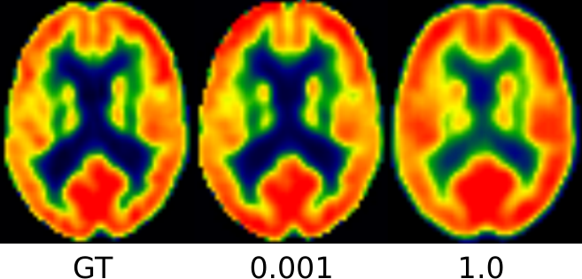
The choice of $\lambda$. $\lambda$ regularizes networks for MRI. Our goal is to model the conditional distribution rather than the joint distribution. A lower weight on this constraint ($0.001$ in all experiments) leads to easier optimization and better qualitative results (Fig 17).

Figure 17: Better for the small $\lambda$.

References

- [1] Martin Arjovsky, Soumith Chintala, and Léon Bottou. Wasserstein gan. arXiv preprint arXiv:1701.07875, 2017.
- [2] John Ashburner, Gareth Barnes, C Chen, Jean Daunizeau, Guillaume Flandin, Karl Friston, Stefan Kiebel, James Kilner, Vladimir Litvak, Rosalyn Moran, et al. Spm12 manual. Wellcome Trust Centre for Neuroimaging, London, UK, 2014.
- [3] Andrew Brock, Jeff Donahue, and Karen Simonyan. Large scale gan training for high fidelity natural image synthesis. arXiv preprint arXiv:1809.11096, 2018.
- [4] Tong Che, Yanran Li, Athul Paul Jacob, Yoshua Bengio, and Wenjie Li. Mode regularized generative adversarial networks. arXiv preprint arXiv:1612.02136, 2016.
- [5] Tianqi Chen, Bing Xu, Chiyuan Zhang, and Carlos Guestrin. Training deep nets with sublinear memory cost. arXiv preprint arXiv:1604.06174, 2016.
- [6] Yunjey Choi, Minje Choi, Munyoung Kim, Jung-Woo Ha, Sunghun Kim, and Jaegul Choo. Stargan: Unified generative adversarial networks for multi-domain image-to-image translation. In Proceedings of the IEEE Conference on Computer Vision and Pattern Recognition, pages 8789–8797, 2018.
- [7] Laurent Dinh, David Krueger, and Yoshua Bengio. Nice: Non-linear independent components estimation. arXiv preprint arXiv:1410.8516, 2014.
- [8] Laurent Dinh, Jascha Sohl-Dickstein, and Samy Bengio. Density estimation using real nvp. arXiv preprint arXiv:1605.08803, 2016.
- [9] Patrick Esser, Ekaterina Sutter, and Björn Ommer. A variational u-net for conditional appearance and shape generation. In Computer Vision and Pattern Recognition, pages 8857–8866, 2018.
- [10] Yaroslav Ganin and Victor Lempitsky. Unsupervised domain adaptation by backpropagation. arXiv preprint arXiv:1409.7495, 2014.
- [11] Abel Gonzalez-Garcia, Joost van de Weijer, and Yoshua Bengio. Image-to-image translation for cross-domain disentanglement. In Advances in Neural Information Processing Systems, pages 1294–1305, 2018.
- [12] Ian Goodfellow, Jean Pouget-Abadie, Mehdi Mirza, Bing Xu, David Warde-Farley, Sherjil Ozair, Aaron Courville, and Yoshua Bengio. Generative adversarial nets. In Advances in neural information processing systems, pages 2672–2680, 2014.
- [13] Xiao Han. Mr-based synthetic ct generation using a deep convolutional neural network method. Medical physics, 44(4):1408–1419, 2017.
- [14] Chris Hinrichs, Vikas Singh, Guofan Xu, and Sterling Johnson. Mkl for robust multi-modality ad classification. In International Conference on Medical Image Computing and Computer-Assisted Intervention, pages 786–794. Springer, 2009.
- [15] Xun Huang, Ming-Yu Liu, Serge Belongie, and Jan Kautz. Multimodal unsupervised image-to-image translation. In European Conference on Computer Vision, pages 172–189, 2018.
- [16] Phillip Isola, Jun-Yan Zhu, Tinghui Zhou, and Alexei A Efros. Image-to-image translation with conditional adversarial networks. In Computer Vision and Pattern Recognition, pages 1125–1134, 2017.
- [17] Jiayin Kang, Yaozong Gao, Feng Shi, David S Lalush, Weili Lin, and Dinggang Shen. Prediction of standard-dose brain pet image by using mri and low-dose brain [18f] fdg pet images. Medical physics, 42(9):5301–5309, 2015.
- [18] Tero Karras, Timo Aila, Samuli Laine, and Jaakko Lehtinen. Progressive growing of gans for improved quality, stability, and variation. arXiv preprint arXiv:1710.10196, 2017.
- [19] Taeksoo Kim, Moonsu Cha, Hyunsoo Kim, Jung Kwon Lee, and Jiwon Kim. Learning to discover cross-domain relations with generative adversarial networks. In International Conference on Machine Learning, pages 1857–1865. JMLR. org, 2017.
- [20] Diederik P Kingma and Jimmy Ba. Adam: A method for stochastic optimization. arXiv preprint arXiv:1412.6980, 2014.
- [21] Durk P Kingma and Prafulla Dhariwal. Glow: Generative flow with invertible 1x1 convolutions. In Advances in Neural Information Processing Systems, pages 10235–10244, 2018.
- [22] Hsin-Ying Lee, Hung-Yu Tseng, Jia-Bin Huang, Maneesh Singh, and Ming-Hsuan Yang. Diverse image-to-image translation via disentangled representations. In European Conference on Computer Vision, pages 35–51, 2018.
- [23] Rongjian Li, Wenlu Zhang, Heung-Il Suk, Li Wang, Jiang Li, Dinggang Shen, and Shuiwang Ji. Deep learning based imaging data completion for improved brain disease diagnosis. In International Conference on Medical Image Computing and Computer-Assisted Intervention, pages 305–312. Springer, 2014.
- [24] Jianxin Lin, Yingce Xia, Tao Qin, Zhibo Chen, and Tie-Yan Liu. Conditional image-to-image translation. In Computer Vision and Pattern Recognition, pages 5524–5532, 2018.
- [25] Ming-Yu Liu, Thomas Breuel, and Jan Kautz. Unsupervised image-to-image translation networks. In Advances in Neural Information Processing Systems, pages 700–708, 2017.
- [26] Ziwei Liu, Ping Luo, Xiaogang Wang, and Xiaoou Tang. Deep learning face attributes in the wild. In International Conference on Computer Vision, pages 3730–3738, 2015.
- [27] Liqian Ma, Xu Jia, Stamatios Georgoulis, Tinne Tuytelaars, and Luc Van Gool. Exemplar guided unsupervised image-to-image translation with semantic consistency. In International Conference on Learning Representations, 2019.
- [28] Matteo Maspero, Mark HF Savenije, Anna M Dinkla, Peter R Seevinck, Martijn PW Intven, Ina M Jurgenliemk-Schulz, Linda GW Kerkmeijer, and Cornelis AT van den Berg. Dose evaluation of fast synthetic-ct generation using a generative adversarial network for general pelvis mr-only radiotherapy. Physics in Medicine & Biology, 63(18):185001, 2018.
- [29] Mehdi Mirza and Simon Osindero. Conditional generative adversarial nets. arXiv preprint arXiv:1411.1784, 2014.
- [30] Sangwoo Mo, Minsu Cho, and Jinwoo Shin. Instance-aware image-to-image translation. In International Conference on Learning Representations, 2019.
- [31] Zak Murez, Soheil Kolouri, David Kriegman, Ravi Ramamoorthi, and Kyungnam Kim. Image to image translation for domain adaptation. In Computer Vision and Pattern Recognition, pages 4500–4509, 2018.
- [32] Dong Nie, Roger Trullo, Jun Lian, Caroline Petitjean, Su Ruan, Qian Wang, and Dinggang Shen. Medical image synthesis with context-aware generative adversarial networks. In International Conference on Medical Image Computing and Computer-Assisted Intervention, pages 417–425. Springer, 2017.
- [33] Aaron van den Oord, Nal Kalchbrenner, and Koray Kavukcuoglu. Pixel recurrent neural networks. arXiv preprint arXiv:1601.06759, 2016.
- [34] Yongsheng Pan, Mingxia Liu, Chunfeng Lian, Tao Zhou, Yong Xia, and Dinggang Shen. Synthesizing missing pet from mri with cycle-consistent generative adversarial networks for alzheimer’s disease diagnosis. In International Conference on Medical Image Computing and Computer-Assisted Intervention, pages 455–463. Springer, 2018.
- [35] Danilo Jimenez Rezende and Shakir Mohamed. Variational inference with normalizing flows. arXiv preprint arXiv:1505.05770, 2015.
- [36] Olaf Ronneberger, Philipp Fischer, and Thomas Brox. U-net: Convolutional networks for biomedical image segmentation. In International Conference on Medical image computing and computer-assisted intervention, pages 234–241. Springer, 2015.
- [37] Apoorva Sikka, Skand Vishwanath Peri, and Deepti R Bathula. Mri to fdg-pet: Cross-modal synthesis using 3d u-net for multi-modal alzheimer’s classification. In International Workshop on Simulation and Synthesis in Medical Imaging, pages 80–89. Springer, 2018.
- [38] John R Silvester. Determinants of block matrices. The Mathematical Gazette, 84(501):460–467, 2000.
- [39] Kihyuk Sohn, Honglak Lee, and Xinchen Yan. Learning structured output representation using deep conditional generative models. In Advances in neural information processing systems, pages 3483–3491, 2015.
- [40] Haoliang Sun, Xiantong Zhen, Chris Bailey, Parham Rasoulinejad, Yilong Yin, and Shuo Li. Direct estimation of spinal cobb angles by structured multi-output regression. In International Conference on Information Processing in Medical Imaging, pages 529–540. Springer, 2017.
- [41] Haoliang Sun, Xiantong Zhen, Yuanjie Zheng, Gongping Yang, Yilong Yin, and Shuo Li. Learning deep match kernels for image-set classification. In Computer Vision and Pattern Recognition, pages 3307–3316, 2017.
- [42] Chaoyue Wang, Chang Xu, Chaohui Wang, and Dacheng Tao. Perceptual adversarial networks for image-to-image transformation. IEEE Transactions on Image Processing, 27(8):4066–4079, 2018.
- [43] Yaxing Wang, Joost van de Weijer, and Luis Herranz. Mix and match networks: encoder-decoder alignment for zero-pair image translation. In Proceedings of the IEEE Conference on Computer Vision and Pattern Recognition, pages 5467–5476, 2018.
- [44] Jelmer M Wolterink, Anna M Dinkla, Mark HF Savenije, Peter R Seevinck, Cornelis AT van den Berg, and Ivana Išgum. Deep mr to ct synthesis using unpaired data. In International Workshop on Simulation and Synthesis in Medical Imaging, pages 14–23. Springer, 2017.
- [45] Minjie Wu, Caterina Rosano, Pilar Lopez-Garcia, Cameron S Carter, and Howard J Aizenstein. Optimum template selection for atlas-based segmentation. NeuroImage, 34(4):1612–1618, 2007.
- [46] Saining Xie and Zhuowen Tu. Holistically-nested edge detection. In International Conference on Computer Vision, pages 1395–1403, 2015.
- [47] Aron Yu and Kristen Grauman. Fine-grained visual comparisons with local learning. In Computer Vision and Pattern Recognition, Jun 2014.
- [48] Aron Yu and Kristen Grauman. Semantic jitter: Dense supervision for visual comparisons via synthetic images. In International Conference on Computer Vision, Oct 2017.
- [49] Jun-Yan Zhu, Taesung Park, Phillip Isola, and Alexei A Efros. Unpaired image-to-image translation using cycle-consistent adversarial networks. In International Conference on Computer Vision, pages 2223–2232, 2017.
- [50] Jun-Yan Zhu, Richard Zhang, Deepak Pathak, Trevor Darrell, Alexei A Efros, Oliver Wang, and Eli Shechtman. Toward multimodal image-to-image translation. In Advances in Neural Information Processing Systems, pages 465–476, 2017.