Dimension constraints improve hypothesis testing for large-scale, graph-associated, brain-image data

Abstract

For large-scale testing with graph-associated data, we present an empirical Bayes mixture technique to score local false discovery rates. Compared to empirical Bayes procedures that ignore the graph, the proposed method gains power in settings where non-null cases form connected subgraphs, and it does so by regularizing parameter contrasts between testing units. Simulations also show that GraphMM controls the false discovery rate in a variety of settings. We apply GraphMM to magnetic resonance imaging data from a study of brain changes associated with the onset of Alzheimer’s disease.empirical Bayes, graph-respecting partition, GraphMM, image analysis, local false discovery rate, mixture model

1 Introduction

The development of empirical Bayesian methods for large-scale hypothesis testing addresses important practical challenges to do with identifying distributional changes while controlling the false discovery rate. Often, these methods are applied relatively late in the data-analysis pipeline, after p-values, test statistics, or other summary statistics are computed for each testing unit. Essentially, the analyst performs univariate testing en masse, with the final unit-specific scores and discoveries dependent upon the choice of empirical Bayesian methodology. Empirical Bayes tools account for the collective properties of the univariate statistics and thereby gain their advantage (e.g., Storey (2003), Efron (2010), Stephens (2017)). These methods may be underpowered in some applied problems when the underlying effects are relatively weak. Motivated by tasks in neuroscience and brain imaging, we describe an empirical-Bayesian approach that operates earlier in the data-analysis pipeline and that leverages regularities achieved through constraining the dimension of the parameter space. Our approach is restricted to data sets in which the variables constitute nodes of a known, undirected graph, which we use to guide regularization. We report simulation and empirical studies with structural magnetic resonance imaging to demonstrate the striking operating characteristics of the new methodology. We conjecture that power is gained for graph-associated data by moving upstream in the data reduction process and by recognizing low complexity parameter states.

The following toy problem illustrates in a highly simplified setting the phenomenon we leverage for improved power. Suppose we have two sampling conditions, and two variables measured each condition, say $X_{1}$ and $X_{2}$ in the first condition and $Y_{1}$ and $Y_{2}$ in the second. We aim to test the null hypothesis that $X_{1}$ and $Y_{1}$ have the same expected value; say $H_{0}:\mu_{X_{1}}=\mu_{Y_{1}}$. Conditional upon target values $\mu_{X_{1}}$, $\mu_{Y_{1}}$ and nuisance mean values $\mu_{X_{2}}$ and $\mu_{Y_{2}}$, the four observations are mutually independent, with normal distributions and some constant, known variance $\sigma^{2}$. We further imagine that these four variables are part of a larger system, throughout which the distinct expected values themselves fluctuate, say according to a standard normal distribution. Within this structure, a test of $H_{0}$ may be based upon the local false discovery rate

$${\rm lfdr}_{1}=P(H_{0}|X_{1},Y_{1})=\frac{p_{0}f(X_{1},Y_{1})}{p_{0}f(X_{1},Y_{1})+(1-p_{0})g(X_{1})g(Y_{2})}$$

where we are mixing discretely over null (with probablity $p_{0}$) and non-null cases. Notice in this setting the across-system variation in expected values may be handled analytically and integrated out; thus in this predictive distribution $g$ is the density of a mean 0 normal distribution with variance $1+\sigma^{2}$; and $f$ is the bivariate normal density with margins $g$ and with correlation $1/(1+\sigma^{2})$ between $X_{1}$ and $Y_{1}$. In considering data $X_{2}$ and $Y_{2}$ on the second variable, it may be useful to suppose that the expected values here are no different from their counterparts on the first variable. We say the variables are blocked if both $\mu_{X_{1}}=\mu_{X_{2}}$ and $\mu_{Y_{1}}=\mu_{Y_{2}}$, and we consider this a discrete possibility that occurs with probablity $p_{\rm block}$ throughout the system, independently of $H_{0}$. In the absence of blocking there is no information in $X_{2}$ and $Y_{2}$ that could inform the test of $H_{0}$ (considering the independence assumptions). In the presence of blocking, however, data on these second variables are highly relevant. Treating blocking as random variable across the system, we would score $H_{0}$ using the local false discovery rate ${\rm lfdr}_{2}=P(H_{0}|X_{1},X_{2},Y_{1},Y_{2})$, which requires consideration of a 4-variate normal and joint discrete mixing over the blocking and null states for full evaluation. Fig. 1 shows the result of simulating a system with $10^{4}$ variable pairs, where the marginal null frequency $p_{0}=0.8$, $\sigma^{2}=1/2$, and the blocking rate $p_{\rm block}$ varies over three possibilities. Shown is the false discovery rate of the list formed by ranking instances by either ${\rm lfdr}_{1}$ or ${\rm lfdr}_{2}$. The finding in this toy problem is that power for detecting differences between $\mu_{X_{1}}$ and $\mu_{Y_{1}}$ increases by accounting for the blocking, since the list of discovered non-null cases by ${\rm lfdr}_{2}$ is larger for a given false discovery rate than the list constructed using ${\rm lfdr}_{1}$. In other words, when the dimension of the parameter space is constrained by blocking, more data become relevant to the test of $H_{0}$ and power increases.

Figure 1: False discovery rate (vertical) as a function of list size (horizontal) for various testing procedures. ${\rm lfdr}_{1}$ refers to the procedure to list the unit if the local false discovery rate $P(\mu_{X_{1}}=\mu_{Y_{1}}|X_{1},Y_{1})$ is sufficiently small (black). Blue lines refer to the operating characteristics when using ${\rm lfdr}_{2}$ which is $P(\mu_{X_{1}}=\mu_{Y_{1}}|X_{1},X_{2},Y_{1},Y_{2})$, for various probabilities $p_{\rm block}$ that the two units share parameters. By accounting for blocking, we benefit through increased yield for a given false-discovery-rate.

Making a practical tool from the blocking observation requires that a number of modeling and computational issues be resolved. Others have recognized the potential, and have designed computationally intensive Bayesian approaches based on Markov chain Monte Carlo (Do and others (2005), Dahl and Newton (2007), Dahl and others (2008), Kim and others (2009)). We seek simpler methodology that may be more readily adapted in various applications. In many contexts data may be organized at nodes of an undirected graph, which will provide a basis for generalizing the concept of blocking using special graph-respecting partitions. Having replicate observations per group is a basic aspect of the data structure, but we must also account for statistical dependence among variables for effective methodology. In the proposed mixture formulation we avoid the product-partition assumption which entails independencies that greatly simplify computations but at the expense of model validity and robustness; we gain numerical efficiency and avoid Markov chain Monte Carlo through a graph-localization of the mixture computations. The resulting tool we call GraphMM, for graph-based mixture model. It is deployed as a freely available open-source R package available at https://github.com/tienv/GraphMM/. We investigate its properties using a variety of synthetic-data scenarios, and we also apply it to identify statistically significant changes in brain structure associated with the onset of mild cognitive impairment.

2 Methods

2.1 Data structure and inference problem

Let $G=(V,E)$ denote a simple, connected, undirected graph with vertex set $V=\{1,2,...,N\}$ and edge set $E$, and consider partitions of $V$, such as $\Psi=\{b_{1},...,b_{K}\}$; that is, blocks (also called clusters) $b_{k}$ constitute non-empty disjoint subsets of $V$ for which $\cup_{k=1}^{K}b_{k}=V$. In the application in Section 3.2, vertices correspond to voxels at which brain-image data are measured, edges connect spatially neighboring voxels, and the partition conveys a dimension-reducing constraint. The framework is quite general and includes, for example, interesting problems from genomics and molecular biology. Recall that for any subset $b\subset V$, the induced subgraph $G_{b}=(b,E_{b})$, where $E_{b}$ contains all edges $e=(v_{1},v_{2})$ for which $e\in E$ and $v_{1},v_{2}\in b$. For use in constraining a parameter space, we introduce the following property: we say that $\Psi$ respects $G$, or that $\Psi$ is graph-respecting, if for all $b_{k}\in\Psi$, the induced graph $G_{b_{k}}$ is connected. Fig.  2 presents a simple illustration.

Figure 2: Examples of partitions on a graph. Different colors represent different blocks. The partition on the left is graph-respecting while the one on the right is not (the blue block induces a subgraph with two components).

It happens that any graph-respecting partition may be encoded with a vector of binary edge variables $Z=\{Z_{e}:e\in E\}$, say with $Z_{e}\in\{0,1\}$. Connected vertices in the same block have $Z_{e}=1$, and those in different blocks have $Z_{e}=0$. For general graphs not every binary edge vector corresponds to a graph-respecting partition, however if $G$ is a tree then the graph-respecting partitions are in one-to-one correspondence with length-$(N-1)$ binary vectors. In case the graph is complete, then the set of possible graph-respecting partitions is the same as the set of all partitions of $V$; i.e. the graph provides no reduction in the complexity of the set of partitions. It becomes relevant to statistical modeling that the size of the set of graph-respecting partitions, though large, still is substantially smaller than the set of all partitions as the graph itself becomes less complex. For example there are 21147 partitions of $N=9$ objects (the 9th Bell number), but if these 9 objects are are arranged as vertices of a regular $3\times 3$ lattice graph, then there are only 1434 graph-respecting partitions. In certain modeling settings, such as with Dirchlet-process mixture models, latent partitions allow for modeling parameter heterogeneity. We use the graph-respecting property to regularize the otherwise unwieldy set of such partitions.

In our setting, the graph $G$ serves as a known object that provides structure to a data set being analyzed for the purpose of a two-group comparison. This is in contrast, for example, to graphical-modeling settings where the possibly unknown graph holds the dependency patterns of the joint distribution. We write the two-group data as $\boldsymbol{X}=(X_{v,m})$ and $\boldsymbol{Y}=(Y_{v,r})$, where $v\in V$, $m=1,\dots,M_{X}$ and $r=1,\dots,M_{Y}$. Here $M_{X}$ and $M_{Y}$ denote the numbers of replicate samples in both groups. In Section 3.2, for example, $m$ indexes the brain of a normal control subject and $r$ indexes the brain of a subject with mild cognitive impairment. For convenience, let $\boldsymbol{X_{m}}=(X_{v,m},\;v\in V)$ and $\boldsymbol{Y_{r}}=(Y_{v,r},\;v\in V)$ denote the across-graph samples on subjects $m$ and $r$, which we treat as identically distributed within group and mutually independent over $m$ and $r$ owing to the two-group, unpaired experimental design.

Our methodology tests for changes between the two groups in the expected-value vectors: $\boldsymbol{\mu_{X}}=E(\boldsymbol{X_{m}})=(\mu_{X_{1}},\dots,\mu_{X_{N}})$ and $\boldsymbol{\mu_{Y}}=E(\boldsymbol{Y_{r}})=(\mu_{Y_{1}},\dots,\mu_{Y_{N}})$. Specifically, we aim to test, for any vertex $v\in V$,

$$H_{0,v}:\mu_{X_{v}}=\mu_{Y_{v}}\,\,\,\textrm{ vs. }\,\,\,H_{1,v}:\mu_{X_{v}}\neq\mu_{Y_{v}}.$$ (2.1)

We seek to gain statistical power over contemporary testing procedures by imposing a dimension constraint on the expected values. Although it is not required to be known or even estimated, we suppose there exists a graph-respecting partition $\Psi=\{b_{k}\}$ that constrains the expected values:

$$\begin{cases}\mu_{X_{v}}=\mu_{X_{u}}\quad\quad\textrm{if for some $k$, both}\,v,u\in b_{k}\\ \mu_{X_{v}}\neq\mu_{X_{u}}\quad\quad\textrm{if}\,v,u\textrm{ belong to different blocks }\end{cases}$$ (2.2)

$$\begin{cases}\mu_{Y_{v}}=\mu_{Y_{u}}\quad\quad\textrm{if for some $k$, both}\,v,u\in b_{k}\\ \mu_{Y_{v}}\neq\mu_{Y_{u}}\quad\quad\textrm{if}\,v,u\textrm{ belong to different blocks }\end{cases}$$

All vertices $v$ in block $b_{k}$ have a common mean in the first group, say $\varphi_{k}$, and a common mean $\nu_{k}$ in the second group. The contrast on test, then, is $\delta_{k}=\nu_{k}-\varphi_{k}$; together with $\Psi$, the binary vector $\boldsymbol{\Delta}=(\Delta_{1},\dots,\Delta_{K})$ holding indicators $\Delta_{k}=1[\delta_{k}\neq 0]$ is equivalent to knowing whether or not $H_{0,v}$ in (2.1) is true for each vertex $v$. When data are consistent with a partition $\Psi$ in which the number of blocks $K$ is small compared to the number of vertices $N$, then it may be possible to leverage this reduced parameter-space complexity for the benefit of hypothesis-testing power.

2.2 Graph-based Mixture Model

2.2.1 Discrete mixing.

We adopt an empirical Bayes, mixture-based testing approach, which requires that for each vertex we compute a local false discovery rate:

$$l_{v}:=P(H_{0,v}|\boldsymbol{X},\boldsymbol{Y})=\sum_{\Psi,\boldsymbol{\Delta}}(1-\Delta_{k})\mathds{1}(v\in b_{k})P(\boldsymbol{\Delta},\Psi|\boldsymbol{X},\boldsymbol{Y}).$$ (2.3)

Our list $\mathcal{L}$ of discovered (non-null) vertices is $\mathcal{L}=\{v:l_{v}\leq c\}$ for some threshold $c$. Conditional on the data, the expected rate of type-I errors within $\mathcal{L}$ is dominated by the threshold $c$ (Efron (2007), Newton and others (2004)). The sum in (2.3) is over the finite set of pairs of partitions $\Psi$ and block-change indicator vectors $\boldsymbol{\Delta}$. This set is intractably large for even moderate-sized graphs. We have experimented with Markov-chain Monte Carlo for general graphs, but present here exact computations in the context of very small graphs. Specifically, for each vertex $v$ in the original graph we consider a small local subgraph in which $v$ is one of the central vertices, and we simply deploy GraphMM on this local graph. Further details are in Supplementary Material.

By summing in (2.3) we perform marginal posterior inference, and thus have a mechanism for borrowing strength among vertices $v$. Of course by Bayes’s rule,

$$P(\boldsymbol{\Delta},\Psi|\boldsymbol{X},\boldsymbol{Y})\propto f(\boldsymbol{X},\boldsymbol{Y}|\boldsymbol{\Delta},\Psi)\,P(\boldsymbol{\Delta},\Psi),$$

and both the prior mass $P(\boldsymbol{\Delta},\Psi)$ and the prior predictive density $f(\boldsymbol{X},\boldsymbol{Y}|\boldsymbol{\Delta},\Psi)$ need to be specified to compute inference summaries. Various modeling approaches present themselves. For example, we could reduce data per vertex to a test statistic (e.g., t-statistic) and model the predictive density nonparametrically, as in the R package locFDR (see Efron (2010)). Alternatively, we could reduce data per vertex less severely, retaining effect estimates and estimated standard errors, as in adaptive shrinkage (Stephens (2017)). In either case we would need to retain information about statistical dependencies between vertices; numerical experiments show that badly mis-specifying this dependence leads to inflated false discovery rate. The approach reported here takes an explicit parametric-model formulation for the predictive distribution of data given the discrete state $(\Psi,\boldsymbol{\Delta})$. This restricts the sampling model to be Gaussian, but allows general covariance among vertices and is not reliant on the product-partition assumption commonly used in partition-based models (Barry and Hartigan (1992)).

In the present work we use a simple specification for $P(\Psi,\Delta)$; namely $P(\Psi)\propto 1$ and $P(\Delta|\Psi)$ encodes independent and identically distributed block-specific Bernoulli$(p_{0})$ indicators of a block shift. In numerical experiments we use univarite empirical-Bayes techniques to estimate $p_{0}$ (Supplementary Material).

2.2.2 Predictive density given discrete structure.

We take a multivariate Gaussian sampling model:

$$\boldsymbol{X_{m}}|\boldsymbol{\mu_{X}},U,\Psi,\boldsymbol{\Delta} \sim_{\rm i.i.d.} \mathcal{N}(\boldsymbol{\mu_{X}},U)\quad\quad m=1,\dots,M_{X}$$

$$\boldsymbol{Y_{r}}|\boldsymbol{\mu_{Y}},W,\Psi,\boldsymbol{\Delta} \sim_{\rm i.i.d.} \mathcal{N}(\boldsymbol{\mu_{Y}},W)\quad\quad r=1,\dots,M_{Y}.$$

We do not constrain the $N\times N$ covariance matrices $U$ and $W$, though we place a conjugage inverse Wishart prior distribution on them:

$$U|\Psi,\boldsymbol{\Delta},\boldsymbol{\mu_{X}},\boldsymbol{\mu_{Y}}\sim\mathcal{IW}(A,\textrm{df}),\qquad W|\Psi,\boldsymbol{\Delta},\boldsymbol{\mu_{X}},\boldsymbol{\mu_{Y}}\sim\mathcal{IW}(B,\textrm{df}).$$

Our predictive densities are conditional on the blocking and change patterns in $\Psi$ and $\boldsymbol{\Delta}$; in general there is no simple conjugate reduction owing to the less-than-full dimension of free parameters in $\boldsymbol{\mu_{X}}$ and $\boldsymbol{\mu_{Y}}$. On these free parameters we further specify independent Gaussian forms:

$$\varphi_{k}\sim\mathcal{N}\left(\mu_{0},\tau^{2}\right),\quad{\rm and}\quad\delta_{k}\sim\mathcal{N}\left(\delta_{0},\sigma^{2}\right)\quad\textrm{ if }\Delta_{k}\neq 0.$$

Hyperparameters in GraphMM include scalars $\delta_{0}$, $\mu_{0}$, $\tau^{2}$, $\sigma^{2}$, df and matrices $A$, $B$, which we estimate from data across the whole graph following the empirical Bayes approach (for details see Supplementary Material).

Model (2.2.2) specifies the joint density $f(\boldsymbol{X},\boldsymbol{Y},\boldsymbol{\mu_{X}},\boldsymbol{\mu_{Y}},U,W|\boldsymbol{\Delta},\Psi)$. For the purpose of hypothesis testing, we need to marginalize most variables, since $H_{0,v}$ is equivalent to $\Delta_{k}=0$ and $v\in b_{k}$ for block $b_{k}$ in partition $\Psi$, and local false discovery rates require marginal posterior probabilities. Integrating out inverse Wishart distributions over the covariance matrices is possible analytically. We find:

$$f(\boldsymbol{X},\boldsymbol{Y}\,\,|\,\,\boldsymbol{\mu_{X}},\boldsymbol{\mu_{Y}},\boldsymbol{\Delta},\Psi) = C\frac{|A|^{\frac{\textrm{df}}{2}}|B|^{\frac{\textrm{df}}{2}}}{|\widetilde{A}|^{\frac{\textrm{{df}}+M_{X}}{2}}|\widetilde{B}|^{\frac{\textrm{{df}}+M_{Y}}{2}}}$$ (2.4)

where

$$C=\dfrac{\Gamma_{N}\left(\frac{\textrm{df}+M_{X}}{2}\right)\Gamma_{N}\left(\frac{\textrm{df}+M_{Y}}{2}\right)}{\pi^{\frac{(M_{X}+M_{Y})N}{2}}\left[\Gamma_{N}(\frac{\textrm{df}}{2})\right]^{2}}\,\,,\,\,\Gamma\textrm{ stands for multivariate gamma function}$$

$$\widetilde{A}=A+(M_{X}-1)S_{1}+M_{X}S_{2}$$

$$S_{1}=\dfrac{1}{M_{X}-1}\sum_{m=1}^{M_{X}}(\boldsymbol{X_{m}}-\overline{\boldsymbol{X}})(\boldsymbol{X_{m}}-\overline{\boldsymbol{X}})^{\tau}$$

$$S_{2}=(\overline{\boldsymbol{X}}-\boldsymbol{\mu_{X}})(\overline{\boldsymbol{X}}-\boldsymbol{\mu_{X}})^{\tau}$$

$$\widetilde{B}=B+(M_{Y}-1)T_{1}+M_{Y}T_{2}$$

$$T_{1}=\dfrac{1}{M_{Y}-1}\sum_{r=1}^{M_{Y}}(\boldsymbol{Y_{r}}-\overline{\boldsymbol{Y}})(\boldsymbol{Y_{r}}-\overline{\boldsymbol{Y}})^{\tau}$$

$$T_{2}=(\overline{\boldsymbol{Y}}-\boldsymbol{\mu_{Y}})(\overline{\boldsymbol{Y}}-\boldsymbol{\mu_{Y}})^{\tau}$$

In the above, notation $|.|$ denotes matrix determinant and $\overline{\boldsymbol{X}}$ and $\overline{\boldsymbol{Y}}$ are sample means

$$\overline{\boldsymbol{X}}=\frac{1}{M_{X}}\sum_{m=1}^{M_{X}}\boldsymbol{X_{m}},\qquad\overline{\boldsymbol{Y}}=\frac{1}{M_{Y}}\sum_{r=1}^{M_{Y}}\boldsymbol{Y_{r}}.$$

Note that $S_{1}$ and $T_{1}$ are sample covariance matrices of $\boldsymbol{X}$ and $\boldsymbol{Y}$ respectively. We using Laplace approximation to numerically integrate the freely-varying means in order to obtain the marginal predictive density $f(\boldsymbol{X},\boldsymbol{Y}|\boldsymbol{\Delta},\Psi)$. Our explicit formula is presented in Supplementary Material.

Notably, by not constraining the sample covariance matrices $U$ and $V$ the GraphMM model does not adopt a product-partition form. In such, the predictive density would factor over blocks in the graph-respecting partition, and this would lead to simpler computations. We found in preliminary numerical experiments that various data sets are not consistent with this simplified dependence pattern, and we therefore propose the general form here. In working on relatively small local graphs the computations remain relatively straightforward in this case.

2.3 Data-driven simulations

Our primary evaluation of GraphMM is through an extensive set of simulations. As we have been motivated by a brain science problem (Section 3.2), we design these simulations to have summary empirical characteristics matching the empirical characteristics of our primary data set (Section 3.2). This data set comes from the Alzheimer’s Disease Neuroimaging Initiative 2 (ADNI-2), and provides a template for the simulation. Briefly, we consider brain MRI data from a group of $M_{X}=123$ normal control subjects (group 1) and a second group of $M_{Y}=148$ subjects suffering from late-stage mild cognitive impairment (late MCI), a precursor to Alzheimer’s disease. The simulation-guiding data involve a single coronal slice with $N=5236$ voxels. Fig. 3 illustrates the general framework for all simulation scenarios; further details are in Algorithm 2, Supplementary Material. We use greedy clustering (Collins, 2014) on the empirical mean profiles to generate blocks for the synthetic expected values, and we adjust the empirical covariances by adding diagonal weight to assure invertibility. Three synthetic data sets are simulated in each scenario. The first three scenarios address the issue of block size; the next two investigate the role of the distribution of condition effects. To assess robustness, we also consider parameter settings where partitions are not graph respecting, and condition effects are not uniform over blocks. We also deploy two permutation experiments; the first uses sample label permutation to confirm the control of the false discovery rate, and the second uses voxel permutation to confirm that sensitivity drops when we disrupt the spatially coordiated signal.

Figure 3: Structure of data-driven simulation (Scenarios 1-5): Steps 1-4 make the correlation structure of synthetic data similar to that of MRI data. Steps 5-7 aim to mimic the mean structure and clustering pattern of MRI data. Steps 8-11 simulate data following multivariate normal distribution with specified correlation and mean structure.

When applying GraphMM to each synthetic data set, we estimate hyperparameters for all distributional components and consider discoveries as ${\mathcal{L}}(c)=\{v:l_{v}\leq c\}$ for various thresholds $c$. We call the controlled FDR the mean $\sum_{v}l_{v}1[v\in{\mathcal{L}}(c)]/\sum_{v}1[v\in{\mathcal{L}}(c)]$, as this is the conditional expected rate of type-1 errors on the list, given data (and computable from data). We know the null status in each synthetic case, and so we also call the empirical FDR to be that rate counting latent null indicators; likewise the true positive rate counts the non-null indicators. We compare GraphMM to several contemporary testing methods, including Benjamini-Hochberg correction (BH adj), Benjamini and Hochberg (1995), local FDR, (locfdr) Efron (2007), and $q$-value (qvalue), Storey (2003), that are all applied to voxel-specific t-tests. We also compare results to adaptive shrinkage, Stephens (2017), both the local FDR statistic (ash_lfdr) and the $q$-value (ash_qval). These methods all work on summaries of voxel-specific tests; summaries may be p-values (for BH and q-value), or t-statistics (for locFDR), or effect estimates and estimated standard errors (for ASH). In any case, none of the methods leverages the graphical nature of the data in the way done by GraphMM.

3 Results

3.1 Operating characteristics of GraphMM

We first do a sanity check to confirm that statistical efficiency gains may arise by regularizing the expected values through the graph-respecting assumption. In a predictive simulation of the $3\times 3$ lattice, we generate synthetic Gaussian data $D$ as follows: expected values are guided by some generative graph-respecting partition $\Psi^{*}$ (drawn from a prior); block-specific means are realized as i.i.d. Gaussian$(0,\sigma^{2}=1/4)$ variables; the 9 data elements in $D$ deviate from these means by realizations of i.i.d. Gaussian$(0,\sigma^{2}=1)$ variables. Each simulated data set is one instance of data when the generative setting is graph-respecting. We take each such simulated data set and work out what two different analysts would surmise about the generative partition. Analyst A knows that the expected values follow some partition structure. Analyst B knows also that the expected values follow a graph-respecting partition. Each analyst computes a posterior distribution, say $P_{\rm analyst}(\Psi|D)$, over the set of partitions; indeed each posterior distribution is concentrated at some level around the generative partition $\Psi^{*}$. A simple measure of the concentration is through the induced distribution on the Adjusted Rand Index, which measures a similarity $S(\Psi,\Psi^{*})$ between two partitions. For any level of similarity, $s$, each analyst has a posterior probability $p_{\rm analyst}(s,D)=P\left[S(\Psi,\Psi^{*})\leq s|D\right]$. Figure 4 compares analysts by the average of these posterior similarity distributions $p_{\rm analyst}(s,D)$ over data sets $D$. It reveals that by enforcing regularity on the prior distribution over partitions (i.e., by enforcing the graph-respecting property), we tend to place greater posterior probability mass near the generative partition. In applications where the graph conveys structure of expected values, the graph-respecting assumption may usefully regularize the local FDR computations to benefit sensitivity.

Figure 4: Shown are predictive averages of posterior similarity distributions between the generative mean partition and the posterior distribution over partitions for two analysts. For each similarity value $s$ (Adjusted Rand Index), each curve records the predictive average $E\left[P(S(\Psi,\Psi^{*})\leq s|D)|{\rm OK}\right]$, where OK is the event that the true partition $\Psi^{*}$ is graph-respecting. One analyst uses a prior that ignores the graph; the other uses a graph-respecting prior. The analyst who has regularized posterior computations tends to place more posterior probability near the generative partition.

Next we address operating characteristics of the GraphMM methodology itself, aiming to find FDR-controlled lists of non-null vertices. Synthetic data sets mimic the structure and empirical characteristics of the brain MRI study data described in Section 3.2. The first three synthetic-data scenarios consider a single MRI brain slice measured on replicates from two conditions, with characteristics approximately matching the characteristics of observed data (Table 2). These scenarios vary the underlying size distribution of blocks, but follow the GraphMM model in having graph-respecting partitions of the underlying signal, block-level shifts between conditions, and multivariate Gaussian errors. The left panel of Figure 5 shows that all methods on test are able to control the false discovery rate. All methods display sensitivity for the signals, though GraphMM demonstrates superior power in the first two cases where blocks extend beyond the individual voxel. The high sensitivity in Scenario 2 may reflect that the prior distribution of block sizes used in the local GraphMM more closely matches the generative situation. Notably, even when this block-size distribution is not aligned with the GraphMM prior, we do not see an inflation of the false discovery rate.

Scenarios 4 and 5 are similar to the first cases, however they explore different forms of signals between the two groups; both have an average block size of 4 voxels, but in one case the changed block effects are fewer, relatively strong and in the other case they are more frequent, and relatively weaker (Table 3). In both regimes, GraphMM retains its control of FDR and exhibits good sensitivity compared to other methods (Fig. 6).

		Scenario 1 12-14 vx/block
		Scenario 2 2-5 vx/block
		Scenario 3 1 vx/block

Figure 5: Operating characteristics on synthetic data. Rows correspond to simulation scenarios (1=top, large blocks; 2=middle, small blocks; 3=bottom, tiny blocks). On the left we compare the empirical FDR with the target controlling FDR. Dominance by the diagonal (black) confirms that all methods are controlling FDR at the target rates. The right panels show how well different methods identify voxels that are truly different between the two groups. Substantial power gains are evident by GraphMM. Table 2 provides simulation details.

		Scenario 4 low frequency large shifts
		Scenario 5 high frequency small shifts

Figure 6: Operating characteristics on synthetic data (Scenarios 4 and 5).

GraphMM is designed for the case where partition blocks are graph respecting and the changes between conditions affect entire blocks. Our next numerical experiment checks the robustness of GraphMM when this partition/change structure is violated Fig. 7 shows that GraphMM continues to control FDR and also retains a sensitivity advantage even when its underlying model is not fully correct.

Figure 7: Robustness to graph-respecting assumption. FDR (left) and sensitivity (right) in a case where latent partitions are not graph respecting, but have similarity 0.48 (Rand index).

To further assess the properties of GraphMM, we performed several permutation experiments. Both started with the data set from Section 3.2. In the first, we simply permuted the sample labels of the 148 control subjects and 123 late MCI subjects, repeating for ten permuted sets. On each permuted set we applied various methods to detect differences. All discoveries are false discoveries in this null case. The left panel of Figure 8 shows that GraphMM and other methods are correctly recognizing the apparent signals as being consistent with the null hypothesis.

The second permutation experiment retains the sample-grouping information, but permutes the voxels within the brain slice on test. This permutation disrupts both spatial measurement dependencies and any spatial structure in the signal. Since GraphMM is leveraging spatially-coherent patterns in signal, we expect it to produce fewer statistically significant findings in this voxel-permutation case. The right panel of Fig. 8 shows this dampening of signal as we expect, when looking at the empirical cdf of computed values $l_{v}=P(H_{0,v}|X,Y)$.

sample label permutation	voxel permutation

Figure 8: Permutation experiments:

3.2 Analysis of Magnetic Resonance Images from the ADNI dataset

The data set used in this section comes from the Alzheimer’s disease Neuroimaging Initiative-II (ADNI-2^∗). Our goal here was two fold:

1. evaluate the sensitivity of our proposal in identifying group-level differences between participants corresponding to different disease stages in a real scientific analysis task, and

2. assess, via scientific interpretation of the results, the extent to which the findings from our analysis is corroborated by known results in the literature on aging and Azheimer’s disease (AD).

The latter sub-goal is feasible because one could utilize standard pre-processing steps, described shortly, on our cohort of brain images and identify the brain regions pertinent to the clinical condition. Since the spatial location of these gray matter anatomical regions can be identified, we can evaluate whether the results are meaningful from the scientific perspective.

Dataset and pre-processing steps used. For the experimental analysis that is presented in this section, gray matter tissue probability maps derived from the co-registered T1-weighted magnetic resonance imaging (MRI) data, downloaded from ADNI using pre-processing steps provided in the commonly used voxel-based morphometry (VBM) toolbox in Statistical Parametric Mapping software (SPM, http://www.fil.ion.ucl.ac.uk/spm). Note that prior to registration to a common template or atlas (which provides a common coordinate system for conducting the analysis), standard artifact removal and other corrections were performed, consistent with existing literature Ithapu and others (2015). Our dataset included brain images of $148$ healthy control subjects (cognitively normal, abbreviated by CN) and $123$ subjects with late mild cognitively impairment (LMCI). We also pre-filter voxels with very low marginal standard deviation (Bourgon and others, 2010), which leaves $464441$ voxels in total. We then apply rank-based inverse normal transformation in order to make data approximately normal.

Analysis task and baselines. Our goal is to detect or identify regions (i.e., voxels) where the distribution of gray matter intensities is significantly different across the clinical conditions, i.e., healthy controls (CN) and late stage Mild Cognitive impaired individuals (LMCI). To keep the computational burden manageable, instead of processing the entire 3D image volume at once, we applied GraphMM (as well as a number of baseline methods) to 2D image slices in the coronal direction. Our baseline methods include Statistical non-parametric Mapping toolbox using Matlab SnPM, a popular image analysis method used by various groups, and $q$-value with adaptive shrinkage using R package ashr, which represents an advanced voxel-specific empirical-Bayes method.

Summary of main experimental findings. Fig. 9 shows a representative example output of our analysis for a montage of 4 coronal slices extracted from the 3D image volume. The color bar (red to yellow), for each method presented, is a surrogate for the strength of some score describing the group-level difference: for instance, for SnPM, the color is scaled based on adjusted $p$-values, for the $q$-value method, it is scaled based on $q$-values, whereas for GraphMM, the color is scaled based on local false discovery rates $l_{v}$. It is clear that while the regions reported as significantly different between CN and LMCI have some overlap between the different methods, GraphMM is able to identify many more significantly different voxels compared to baseline methods, at various FDR thresholds (Fig. 11). A closer inspection of one case is informative (Fig.10). 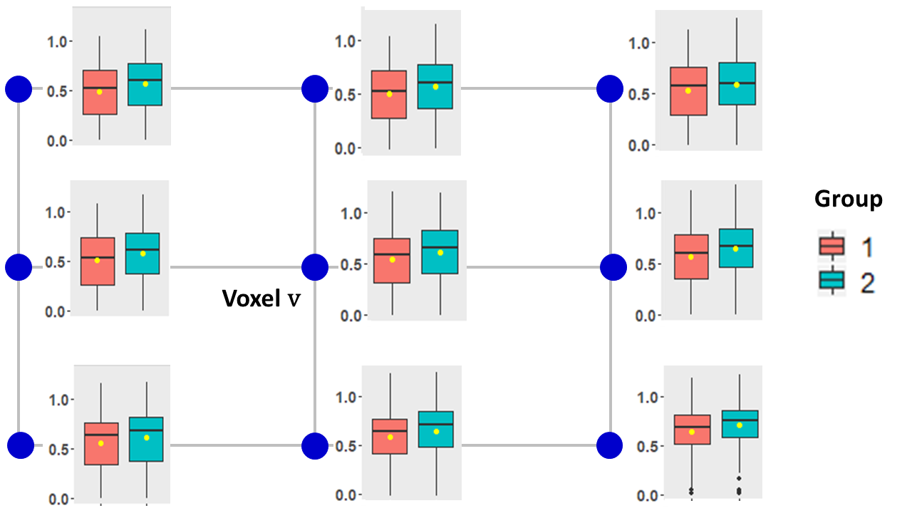Voxel $v$ at coordinates $(x=31,y=53,z=23)$ is not found to be different between CN and MCI according to SnPM (adjusted $p$-value = 0.578) and $q$-value method ($q$-value = 0.138). But when we look at the results provided by GraphMM, the local FDR is $0.001$. It is clear that part of the reason behind the increased sensitivity is that GraphMM is leveraging the consistent pattern of shifts among neighboring voxels.

Figure 9: Figure shows significantly different voxels at 5% FDR (colored area) for 4 coronal slices, found by Statistical non-parametric mapping (SnPM), adaptive shrinkage (ASH) and the proposed GraphMM.

Figure 10: Boxplots for voxel $v$ at coordinates $(x=31,y=53,z=23)$ and its neighbors. Voxel $v$ is altered according to GraphMM but not according to SnPM or $q$-value. Similar shifts nearby $v$ lead to the increased evidence reported by GraphMM.

Clusters. Another statistical measure often reported in the neuroimaging literature is the size of significant clusters, where clusters refer to spatially connected set of voxels that are significantly altered by the sampling condition (e.g., clinical condition). The rational here is that stray voxels reported as significantly different are more likely to be an artifact relative to a group of anatomically clustered voxels. In the literature, results are often reported for clusters with size greater than or equal to 20. In the setting of graph-associated data, a significant cluster forms a connected component of the 3-dimensional lattice graph associated with the data. Fig. 12 shows a bar plot for the size of significant cluster. Here, we see that GraphMM performs favorably relative to the baseline methods and consistently reports larger clusters.

Figure 11: Plot of Controlled FDR vs. Number of significant voxels on the whole brain data. The figure confirms the high yield of GraphMM.

Figure 12: Bar plot for summary on the size of significant clusters. By definition, a significant region is a collection of significant voxels that is spatially connected.

Scientific interpretation of the results. To better interpret the statistical results, we use the Matlab package xjview to link anatomical information associated with those voxels that reported to be significantly different by the various methods. The xjview package maps the significant clusters from the analysis to the brain template or atlas (i.e., common coordinate system) using automated anatomical labeling information (Tzourio-Mazoyer and others, 2002). This is helpful because one can then easily assign anatomically meaningful names to the voxel clusters that are significantly different. The results are summarized in Table 1 where we report the brain regions associated with significant findings from GraphMM as well as SnPM. Specifically, Column 3 in the table provides comparisons from both methods listing the number of significant voxels in the corresponding regions. This process provides additional evidence to assess if our analysis indeed revealed regions known to be associated with AD. We can answer this question by inspecting the neurological functions of the identified brain regions shown in column 4. Here, we only show the top 15 brain regions that contain most number of significant voxels. From Table 1, we see that GraphMM discovers all the brain regions found by SnPM, with many more significant voxels in each region with more pronounced evidence of statistical significance. The only exception is the hippocampus where both methods identify a large number of voxels but GraphMM finds fewer significant voxels than SnPM. In addition, there are regions revealed to be significant by GraphMM but not by SnPM, including the precentral gyrus, middle frontal gyrus, inferior frontal gyrus opercular, insular, anterior cingulate, and supramarginal gyrus, which are relevant in the aging and AD literature. GraphMM consolidates known alterations between CN and LMCI and reveals potentially important new findings.

Table 1: Brain regions with significant ( 5% FDR ) change in gray matter volume. found by GraphMM.

No.	Brain region	# Voxels  GraphMM     SnPM	Neurological function
1	Hippocampus	1411 1646	Receives and consolidates new memory about experienced events, allowing for establishment of long-term memories. [Cohen and Eichenbaum (1993)]
2	Parahippocampal Gyrus	1008 410	Involved in episodic memory and visuospatial processing [Aminoff and others (2013)].
3	Amygdala	710 365	Plays an essential role in the processing and memorizing of emotional reactions [Knafo (2012)]
4	Temporal Gyrus (superior, middle and inferior)	2031 287	Involved in various cognitive processes, including language and semantic memory processing (middle) as well as visual perception (inferior) and sound processing (superior) [Onitsuka and others (2004), Bigler and others (2007)]
5	Putamen	793 12	Linked to various types of motor behaviors, including motor planning, learning, and execution.[Marchand and others (2008)].
6	Fusiform Gyrus	735 308	Influence various neurological phenomena including face perception, object recognition, and reading [Weiner and Zilles (6 03)].
7	Temporal Pole (superior, middle)	882 74	Involved with multimodal analysis, especially in social and emotional processing. [Plotzker and others (2007)].
8	Precentral Gyrus	829 0	Consists of primary motor area, controlling body’s movements. [Graziano and others (2002)].
9	Middle Frontal Gyrus	635 0	Plays essential role in attentional reorienting. [Japee and others (2015)].
10	Inferior Frontal Gyrus Opercular	573 0	Linked to language processing and speech production. [Greenlee and others (2007)].
11	Calcarine	381 22	Where the primary visual cortex is concentrated, processes visual information. [Meadows (2011)].
12	Caudate	437 46	Plays essential roles in motor processes and a variety of executive, goal-directed behaviours [Grahn and others (2008)].
13	Insular	275 0	Involved in consciousness, emotion and the regulation of the body’s homeostasis [Gogolla (2017)].
14	Anterior Cingulate	260 0	Plays a major role in mediating cognitive influences on emotion. [Stevens and others (2011)].
15	Supramarginal Gyrus	225 0	Linked to phonological processing and emotional responses. [Hartwigsen and others (2010)].

4 Discussion

Mass univariate testing remains the dominant approach to detect statistically significant changes in comparative brain-imaging studies (e.g., Groppe and others (2011)). Here, a classical testing procedure, like the test of a contrast in a regression model, is applied in parallel over all testing units (voxels), leading to a large number of univariate test statistics and p-values. Subsequently, significant voxels are identified through some filter, such as the Benjamini-Hochberg (BH) procedure, that aims to control the false discovery rate. The approach is often very effective and has supported numerous important applied studies of brain function. In structural magnetic resonance image studies of Alzheimer’s disease progression, such mass univaraiate testing has failed in some cases to reveal subtle structural changes between phenotypically distinct patient populations. The underlying problem is limited statistical power for relatively small effects, even with possibly hundreds of subjects per group. Empirical Bayes procedures improve power somewhat over BH by recognizing properties of the collection of tests. In case the data are associated with a graph and are consistent with a relatively low dimension of parameter states, we have shown one way to further enhance the empirical Bayes procedures.

Empirical Bayesian procedures trace their beneficial operating characteristics to “information sharing”, or, equivalently, “borrowing strength”. In isolation, the parameters governing data at a given testing unit are inferred locally from data at that unit. Having limited data at each unit limits any inferences we may try to make. But in treating the unit-level parameters – considered over many units – as draws from some common, system-level population of parameters, Bayesian theory provides a formal approach to link information between units (e.g., Bernardo and Smith (1994)). Relatively elaborate information sharing is provided by highly flexible Bayesian models. For example, the Dirichlet process mixture (DPM) model engenders a clustering of the inference units, with units in the same cluster block if (and only if) they share the same parameter values. The DPM model has been effective at representing heterogeneity in a system of parameters (e.g., Muller and Quintana (2004)), and in improving sensitivity in large-scale testing (e.g., Dahl and Newton (2007), Dahl and others (2008)). Benefits come at a high computational cost, since in principle the posterior summaries require averaging over all partitions of the units (e.g., Blei and Jordan (2006)). There are also modeling costs: DPM’s usually have a product-partition form in which the likelihood function factors as a product over blocks of the partition (Hartigan (1990)). In applications, such as brain imaging, we observe that independence between blocks is violated in a way that may lead to inflation of the actual false discovery rate over a target value.

The application of main focus in our research is structural magnetic resonance imaging (sMRI) data that arise in studies of brain structure and function. sMRI provides information to describe the shape, size, and integrity of brain structures. Briefly, the contrast and brightness of structural magnetic resonance images is determined by the characteristics of brain tissues. Depending on the types of sMRI sequences (e.g, T1-weighted, T2-weighted, proton density-weighted), different aspects of brain tissues are emphasized. We are particularly interested in T1-weighted sMRI, which provides good contrast between gray matter tissue (darker gray) and white matter tissue (lighter gray), while the cerebrospinal fluid is void of signal (black). Because brain function depends to some extent on the integrity of brain structure, sMRI has become an integral part for clinical assessment of patients with suspected Alzheimer’s disease (Vemuri and Jack (2010)). By studying structural magnetic resonance images, we are able to make inference about gray matter atrophy in the brain, which has been shown to be one of classic symptoms for Alzheimer’s disease (AD) in the neuroscience literature (e.g., Frisoni and others (2002), Scheltens and others (2002), Moller and others (2013)). Essentially, conclusions regarding the atrophy of gray matter may come from detecting changes in gray matter volume across different stages of Alzheimer’s degenerative process. Furthermore, identifying subtle changes at early stages could help with early detection of gray matter atrophy, which ultimately facilitates AD diagnosis, interventions and treatments.

The crux of methodological research on large-scale testing in neuroimaging has been how to find thresholds on voxel-wise test statistics that control a specified false positive rate and maintain testing power. The two approaches that are most popular to neuroimaging researchers include: family-wise error control using Random Field Theory (e.g., Worsley and others (2004)) and false discovery rate control using Benjamin-Hochberg procedure (e.g., Genovese and others (2002)). The former is based on additional assumptions about the spatial smoothness of the MRI signal. There have been criticisms. e.g., in Eklund and others (2016), that these smoothness assumptions are usually not satisfied by the data, which would lead to alarmingly high degree of false positive. The voxel-wise test statistic can be either parametric (implemented in SPM Matlab package Penny and others (2007)) or non-parametric (implemented in Statistical Nonparametric mapping (SnPM) Matlab toolbox Nichols (2001)). A review of available methods for large-scale testing in neuroimaging inference can be found in Nichols (2012) and the references therein. Tansey and others (2018) presented an FDR tool that processes unit-specific test statistics in a way to spatially smooth the estimated prior proportions. As the clinical questions of interest move towards identifying early signs of AD, the changes in average brain profiles between conditions invariably become more subtle and increasingly hard to detect; the result is that very few voxels or brain regions may be detected as significantly different by standard methods. The methodology we study in this thesis aims to increase the sensitivity of large-scale tests for neuroimaging and related data.

Graphs provide powerful tools for representing diverse patterns of interactions between entities of a system and have been widely used for modeling data arising in various fields of science (e.g., Gross and Yellen (2004)). In the present work, vertices of the graph correspond to variables in a data set and the undirected edges convey relational information about the connected variables, due to associations with the context of the data set, such as temporal, functional, spatial, or anatomical information. The graphs we consider constitute an auxiliary part of observed data. For clarity, these graphs may or may not have anything to do with undirected graphical representations of the dependence in a joint distribution (e.g. Lauritzen (1996)), as in the graphical models literature. For us, the graph serves to constrain patterns in the expected values of measurements. By limiting changes in expected values over the graph, we aim to capture low complexity of the system. An alternative way to model low-complexity is through “smoothed/bandlimited” signals (e.g., Ortega and others (2018), Chen and others (2016)). Comparisons between the approaches are warranted.‘

We have advanced the idea of latent graph-respecting partitions that constrain expected values into low-dimensional space. The partition is paired with a vector of block-specific change indicators to convey the discrete part of the modeling specification. We used a uniform distribution over graph-respecting partitions in our numerical experiments, and have also considered more generally the distribution found by conditioning a product partition model (PPM) to be graph-respecting. In either case, two vertices that are nearby on the graph are more likely to share expected values, in contrast to the exchangeability inherent in most partition models. Graph restriction greatly reduces the space of partitions; we simply enumerated all such partitions in our proposed graph-local computations and thereby avoided MCMC over partition space. When the generative situation is similarly graph restricted, we expect improved statistical properties; but we also showed that false discovery rates are controlled even if the generative situation is not graph respecting. Special cases of graph-restricted partitions have been studied by others. When $G$ is a lattice graph, we have induces a spatial random partition distribution, which is the topic of study in Page and Quintana (2016). When $G$ is a decomposable graph, the random partition distribution proposed here and the one introduced in Caron and Doucet (2009) are similar in the sense that they are both restricted only on the set of graph-respecting partitions. For a general graph $G$, the distance dependent Chinese restaurant process (ddCPR) introduced in Blei and Frazier (2011) can induce a partition distribution that is also restricted on the graph-respecting partitions, though it differs from the distributions used here. When $G$ is a complete graph there is no restriction and all partitions have positive mass. When $G$ is a line graph the graph-respecting partition model matches Barry and Hartigan (1992) for change-point analysis.

Supplementary Material

Local approximation

Our model considers a general correlation structure. Therefore, it is impractical to apply the model on the entire graph due to high dimensionality. Instead, we derive a divide and conquer heuristic strategy, called local approximation, to overcome computational obstacle, which can take advantage of parallel computing. For each node $v$, consider a neighborhood $\mathcal{N}_{v}$ of node $v$. $\mathcal{N}_{v}$ is chosen such that it is a connected component of graph G. GraphMM, then, is applied to model the data in this neighborhood

$$(\boldsymbol{X_{\mathcal{N}_{v}}},\boldsymbol{Y_{\mathcal{N}_{v}}}):=\{(\boldsymbol{X_{u}},\boldsymbol{Y_{u}}):u\in\mathcal{N}_{v}\}$$

The node-specific posterior probabilities (2.3) is approximated by

$$l_{v}:=P(H_{0,v}|\boldsymbol{X_{\mathcal{N}_{v}}},\boldsymbol{Y_{\mathcal{N}_{v}}})=\sum_{\Psi,\boldsymbol{\Delta}}\mathds{1}({\Delta_{k}=0})1(v\in b_{k})P(\boldsymbol{\Delta},\Psi|\boldsymbol{X_{\mathcal{N}_{v}}},\boldsymbol{Y_{\mathcal{N}_{v}}})$$ (4.1)

The local approximation procedure is illustrated by Fig. 13.

Figure 13: Illustration for local approximation pipeline. (a) shows pre-processed MRI images of two conditions. (b) shows lattice graphs associated with the data. (c) shows local approximation procedure, in which neighborhood $\mathcal{N}_{v}$ of node $v$ includes $v$ and eight adjacent nodes. GraphMM model is applied to neighborhood data to get approximated posterior probability of null effects $l_{v}$ as in (4.1).

Algorithm 1 Local approximation

1: pre-processed MRI data $\boldsymbol{X}$, $\boldsymbol{Y}$.

2: per voxel posterior probability of differential structure.

3: procedure GraphMM($\boldsymbol{X}$, $\boldsymbol{Y}$)

4:   for $v$ in nodes do

5:    $G_{\textrm{local}}$ $\leftarrow$ local graph around $v$

6:    $(\boldsymbol{X_{\mathcal{N}_{v}}},\boldsymbol{Y_{\mathcal{N}_{v}}})\leftarrow$ local data around $v$

7:    $hyp$ $\leftarrow$ estimated hyperparameters($\boldsymbol{X_{\mathcal{N}_{v}}},\boldsymbol{Y_{\mathcal{N}_{v}}}$)

8:    for $(\Psi,\boldsymbol{\Delta})$ in graph-respecting partitions of $G_{\textrm{local}}$ do

9:      $p(\boldsymbol{X_{\mathcal{N}_{v}}},\boldsymbol{Y_{\mathcal{N}_{v}}}|\Psi,\boldsymbol{\Delta})$ $\leftarrow$ marginal density of data local to $v$

10:      $p(\Psi,\boldsymbol{\Delta})$ $\leftarrow$ prior mass of local state.

11:    end for

12:    Scale to get $p(\Psi,\boldsymbol{\Delta}|\boldsymbol{X_{\mathcal{N}_{v}}},\boldsymbol{Y_{\mathcal{N}_{v}}})$ for all graph-respecting partitons $(\Psi,\boldsymbol{\Delta})$

13:    $l_{v}$ $\leftarrow$ $P(H_{0,v}|\boldsymbol{X_{\mathcal{N}_{v}}},\boldsymbol{Y_{\mathcal{N}_{v}}}))$ # Using formula 4.1

14:   end for

15: end procedure

For results in Sections 3.1 and 3.2, we did local approximation on a $3\times 3$ neighborhood of each node, as illustrated in Fig. 13. In this case we can enumerate all the graph-respecting partitions (we devised a data-augmentation sampling scheme that makes use of spanning trees within the input graph; not shown). Then, we are able to enumerate all the pairs $(\Psi,\boldsymbol{\Delta})$ and compute the exact posterior distribution.

Simulation study details

Algorithm 2 General framework for all the simulation scenarios

1: MRI dataset for condition 1, G1, a $N\times M_{X}$ matrix; real dataset for condition 2, G2, a $N\times M_{Y}$ matrix.

2: synthetic dataset 1 $\boldsymbol{X}$; synthetic dataset 2 $\boldsymbol{Y}$.

3:

4: $S_{1}$ $\leftarrow$ sample-covariance(G1).

5: $S_{2}$ $\leftarrow$ sample-covariance(G2).

6: $\textbf{V}\leftarrow S_{1}+0.5\textbf{I}$ # 82.92189pt I is identity matrix.

7: $\textbf{W}\leftarrow S_{2}+0.5\textbf{I}$ # Add a small value to the diagonal of $S_{1},S_{2}$ to get positive definite matrices.

8: $Avg\leftarrow$ average-over-replicate(G1, G2) # 108.5843pt $Avg$ is a vector of length $N$                 

9:

10: ##### Implement for step 6 to 9 depends on specific scenario #####

11: $\Psi\leftarrow$ cluster($Avg$) # $\Psi=\{b_{1},\dots,b_{K}\}$ is a graph-respecting partition on $Avg$

12: $\boldmath{\Delta}\leftarrow$ changed-block indicator # $\boldmath{\Delta}=\{\Delta_{1},...,\Delta_{K}\}$ is a binary vector, $\Delta_{k}=1$ iff $b_{k}$ is a changed-block.

13:

14:

15: # $\delta_{k}=0$ iff $\Delta_{k}=0$; when $\Delta_{k}\neq 0$, $\delta_{k}$ is simulated from some distribution (e.g beta, uniform)

16: # $\nu$ is simulated block means for condition 2.

17:

18: # $\boldmath{\mu_{X}},\boldmath{\mu_{Y}}$ satisfy clustering constraints on the means w.r.t $\Psi$ as in (2.2).

19:

20: ##########

21: $\boldsymbol{X}\leftarrow$ Multivariate Normal ($\mu_{X},\textbf{V}$)

22: $\boldsymbol{Y}\leftarrow$ Multivariate Normal ($\mu_{Y},\textbf{W}$)

Table 2: Description for simulation 1, 2 and 3. Text with blue color and figures emphasizes that these simulations differ in the average size of latent blocks. In the figures, area with magenta color shows changed-blocks. We can see that the size of changed-blocks decreases in simulation 1, 2 and 3. Especially simulation 3 has no clustering effect, i.e the block size is 1 for all blocks.

	Scenario 1	Scenario 2	Scenario 3
Step 6	* Use greedy clustering method [Collins (2014)] * Partition is adjusted to respect lattice graph. * There are 1313 blocks, average block size is 3.9	Same as scenario 1	* Each node itself is a block. * There are 5236 blocks, block size is 1
Step 7	* 50 blocks with size from 12 to 14 are chosen to be changed-block * Average size of changed-block is 13.6 * Percentage of changed-nodes: 14.3%	* 300 blocks with size from 2 to 5 are chosen to be changed-block * Average size of changed-block is 2.6 * Percentage of changed-nodes: 14.9%	* 15% of the nodes are chosen to be changed-nodes
Step 8, 9	$m_{x}$ $\leftarrow$ block average of MRI data group 1 $m_{y}$ $\leftarrow$ block average of MRI data group 2 $max.d\leftarrow$ max($m_{y}-m_{x}$) $min.d\leftarrow$ min($m_{y}-m_{x}$) $\varphi\leftarrow m_{x}$ For changed-blocks: $\delta\sim$ Uniform($min.d,max.d$)	Same as scenario 1	$m_{x}$ $\leftarrow$ block average of MRI data group 1 $sd_{x}$ $\leftarrow$ sample block standard deviation group 1 $mar.m\leftarrow$ mean($m_{x}$) $mar.sd\leftarrow$ mean($sd_{x}$) $\varphi\sim$ Normal($mar.m,mar.sd$) $m_{y}$ $\leftarrow$ block average of MRI data group 2 $max.d\leftarrow$ max($m_{y}-m_{x}$) $min.d\leftarrow$ min($m_{y}-m_{x}$) For changed-blocks: $\delta\sim$ Beta(2, 2) $\delta\leftarrow\delta*(max.d-min.d)+min.d$
Figure

Table 3: Description for simulation 4 and 5. Text with blue color and figures emphasizes that these simulations differ in the percentage of changed-nodes. The figures show histogram of block avergage shifts across 2 groups for all blocks (red area) and for changed-blocks (green area).

	Simulation 4	Simulation 5
Step 6	* Use greedy clustering method [Collins (2014)] * Partition is adjusted to respect lattice graph. * There are 1313 blocks, average block size is 3.9	Same as Simulation 4
Step 7	$m_{x}$ $\leftarrow$ block average of MRI data group 1 $m_{y}$ $\leftarrow$ block average of MRI data group 2 $diff\leftarrow m_{y}-m_{x}$ $prob\leftarrow$ increasing function of $|diff|$ and belongs in (0,1) $\Delta\sim$ Bernoulli($prob$) * Percentage of changed-nodes: 16.4%	* Similar to simulation 4, except that * Percentage of changed-nodes: 50.3%
Step 8 & 9	* If block $k$ is a changed-block: $\varphi[k]\leftarrow m_{x}[k]$ $\delta[k]\leftarrow diff[k]$ * If block $k$ is not a changed-block: $\varphi[k]\leftarrow(m_{x}[k]+m_{y}[k])/2$ $\delta[k]\leftarrow 0$	Same as Simulation 4
Figure

The graph associated with data is a lattice graph representing spatial dependence, in which the vertices are the pixels and the edges connect neighboring voxels. The analysis of GraphMM involves estimating hyper parameters: prior null probability $p_{0}$, prior mean $\mu_{0}$ and standard deviation $\tau^{2}$ of block mean of group 1, prior mean $\delta_{0}$ and standard deviation $\sigma^{2}$ of difference in block mean between 2 groups, prior covariance matrix $A$ for group 1 and matrix $B$ for group 2. Different strategies for estimating hyperparameters have been considered,

• Estimating prior null probability $p_{0}$: We experimented with both qvalue or ahsr to get the estimated value of $p_{0}$. Package qvalue produces conservative estimate of $p_{0}$ without any assumption on the distribution of effects. Hence it is a safe and conservative choice under general settings. Package ashr, on the other hand, provides conservative estimate under the assumption that the distribution of effects is unimodal. This unimodal assumption has been discussed intensively in Stephens (2017) and has been argued to be both plausible and beneficial in many contexts. Furthermore, in our graph-based mixture model 2.2, the distribution of effects $\delta_{k}$ was assumed to be a mixture of probability mass at 0 and normal distribution, which satisfies unimodal assumption. Therefore, using package ashr to estimate for $p_{0}$ meshes with our GraphMM. The estimation of $p_{0}$ is based on the whole dataset, computing prior to the local approximation procedure. In reported computations we used ashr package for $p_{0}$.

• Estimating other hyperparameters: We consider 3 approaches: global, local and mixed estimation. With global estimation, the hyperparameters are estimated using the whole dataset and computed prior to the local approximation procedure. With local estimation, hyperparameters are estimated for each neighborhood, during the local approximation procedure. With mixed estimation, all hyperparameters are estimated locally except for matrices $A$ and $B$, which are estimated globally. These approaches, local, mixed and global provides increasingly conservative estimates in that order. In following simulation and application, we present results using mixed estimation.

Computing marginal likelihood

We derive the marginal likelihood using Laplace approximation. Consider the notations as in section 2.2. Let $K_{\Psi}$ be the number of blocks corresponding to partition $\boldsymbol{\Psi}$ and $K_{\textrm{diff}}$ be the number of changed blocks, which means

$$K_{\textrm{diff}}=\sum_{k=1}^{K_{\Psi}}\mathds{1}({\Delta_{k}=1})$$

Denote the ordered indices of changed blocks as $(j_{1},j_{2},\dots,j_{K_{\textrm{diff}}})$. We re-parametrize the model in order to remove the clustering constraints on the means

$$\boldsymbol{\epsilon}:=(\delta_{j_{1}},\delta_{j_{2}},\dots,\delta_{j_{K_{\textrm{diff}}}})$$

Then, the free parameters are $(\boldsymbol{\varphi},\boldsymbol{\epsilon})$ and the marginal likelihood function can be written as

$$f(\boldsymbol{X},\boldsymbol{Y}|\boldsymbol{\Psi},\boldsymbol{\Delta}) = \int f(\boldsymbol{X},\boldsymbol{Y},\boldsymbol{\varphi},\boldsymbol{\boldsymbol{\epsilon}}|\boldsymbol{\Psi},\boldsymbol{\Delta})\rm{dP}(\boldsymbol{\varphi})\rm{dP}(\boldsymbol{\epsilon})$$

$$= C_{1}C_{2}\int_{\mathbb{R}^{K_{\Psi}+K_{\textrm{diff}}}}\exp\left[(\textrm{df}+M_{X})F(\boldsymbol{\varphi},\boldsymbol{\epsilon})\right]\rm{d}\boldsymbol{\varphi}~\rm{d}\boldsymbol{\epsilon}$$

where

$$C_{1}=C_{1}(N,M_{X},M_{Y},\textrm{df})=\dfrac{(|A||B|)^{\frac{d}{2}}\Gamma_{N}\left(\frac{\textrm{df}+M_{X}}{2}\right)\Gamma_{N}\left(\frac{\textrm{df}+M_{Y}}{2}\right)}{\left[\Gamma_{N}\left(\frac{\textrm{df}}{2}\right)\right]^{2}}$$

$$C_{2}=C_{2}(\boldsymbol{\Psi},\boldsymbol{\Delta},\tau,\sigma)=\exp\left[-K_{\Psi}\log(\tau\sqrt{2\pi})-K_{\textrm{diff}}\log(\sigma\sqrt{2\pi})\right]$$

$$F(\boldsymbol{\varphi},\boldsymbol{\delta}) = -\dfrac{1}{2}\log|\widetilde{A}|-\dfrac{\textrm{df}+M_{Y}}{2(\textrm{df}+M_{X})}\log|\widetilde{B}|-\dfrac{1}{2\tau^{2}(\textrm{df}+M_{X})}\sum_{k=1}^{K_{\Psi}}(\varphi_{k}-\mu_{0})^{2}$$

$$-\dfrac{1}{2\sigma^{2}(\textrm{df}+M_{X})}\sum_{l=1}^{K_{\textrm{diff}}}(\epsilon_{l}-\delta_{0})^{2}$$

$$\widetilde{A}=A+(M_{X}-1)S_{1}+M_{X}S_{2}$$

$$S_{1}=\dfrac{1}{M_{X}-1}\sum_{m=1}^{M_{X}}(\boldsymbol{X_{m}}-\overline{\boldsymbol{X}})(\boldsymbol{X_{m}}-\overline{\boldsymbol{X}})^{\tau}$$

$$S_{2}=(\overline{\boldsymbol{X}}-\boldsymbol{\mu_{X}})(\overline{\boldsymbol{X}}-\boldsymbol{\mu_{X}})^{\tau}$$

$$\widetilde{B}=B+(M_{Y}-1)T_{1}+M_{Y}T_{2}$$

$$T_{1}=\dfrac{1}{M_{Y}-1}\sum_{r=1}^{M_{Y}}(\boldsymbol{Y_{r}}-\overline{\boldsymbol{Y}})(\boldsymbol{Y_{r}}-\overline{\boldsymbol{Y}})^{\tau}$$

$$T_{2}=(\overline{\boldsymbol{Y}}-\boldsymbol{\mu_{Y}})(\overline{\boldsymbol{Y}}-\boldsymbol{\mu_{Y}})^{\tau}$$

Apply Laplace’s approximation, we get

$$~~~\log f(\boldsymbol{X},\boldsymbol{Y}|\boldsymbol{\Psi},\boldsymbol{\Delta}) \approx \log C_{1}+\log C_{2}+\dfrac{K_{\Psi}+K_{\textrm{diff}}}{2}\log\dfrac{2\pi}{\textrm{df}+M_{X}}$$ (4.2)

$$+(\textrm{df}+M_{X})\textit{F}(\widehat{\boldsymbol{\varphi}},\widehat{\boldsymbol{\epsilon}})-\dfrac{1}{2}\log\left|-\textit{H(F)}(\widehat{\boldsymbol{\varphi}},\widehat{\boldsymbol{\epsilon}})\right|$$

In the next step, we derive the explicit formula for the gradient and Hessian matrix of $F$. Let $L$ be the allocation matrix with size $N\times K_{\Psi}$ where $c_{vk}=1$ if and only iff node $v$ belong to block $k$. Let $R$ be a $K_{\Psi}\times K_{\textrm{diff}}$ matrix such that column $l$th of $R$ has value $1$ at position $j_{l}$ and has value $0$ at other postions. Then we can relate the mean vectors with the new parameters $(\boldsymbol{\varphi},\boldsymbol{\epsilon})$ as follows

$$\boldsymbol{\delta}=R\boldsymbol{\epsilon}$$

$$\boldsymbol{\mu_{X}}=L\boldsymbol{\varphi}~~~~~~\boldsymbol{\mu_{Y}}=L(\boldsymbol{\varphi}+\boldsymbol{\delta})$$

We consider following notations.

$$S_{3}=\dfrac{1}{M_{X}-1}A+S_{1}~~~~~~~~T_{3}=\dfrac{1}{M_{Y}-1}B+T_{1}$$

$$v_{X}=S_{3}^{-1}\overline{\boldsymbol{X}}~~~~~~~~v_{Y}=T_{3}^{-1}\overline{\boldsymbol{Y}}$$

$$s_{0}=\dfrac{M_{X}-1}{M_{X}}+\overline{\boldsymbol{X}}^{\tau}v_{X}~~~~~~~~t_{0}=\dfrac{M_{Y}-1}{M_{Y}}+\overline{\boldsymbol{Y}}^{\tau}v_{Y}$$

$$Q_{X}=L^{\tau}S_{3}^{-1}L~~~~~~~~Q_{Y}=L^{\tau}T_{3}^{-1}L$$

$$w_{X}=S_{3}^{-1}\boldsymbol{\mu_{X}}~~~~~~~~w_{Y}=T_{3}^{-1}\boldsymbol{\mu_{Y}}$$

$$u_{X}=L^{\tau}(w_{X}-v_{X})~~~~~~~~u_{Y}=L^{\tau}(w_{Y}-v_{Y})$$

$$b_{X}=\dfrac{1}{s_{0}-2{v_{X}}^{\tau}\boldsymbol{\mu_{X}}+\boldsymbol{\mu_{X}}^{\tau}w_{X}}$$

$$b_{Y}=\dfrac{1}{t_{0}-2{v_{Y}}^{\tau}\boldsymbol{\mu_{Y}}+\boldsymbol{\mu_{Y}}^{\tau}w_{Y}}$$

The formula for the gradient of $F$ is.

$$\dfrac{\partial F}{\partial\boldsymbol{\varphi}}=\left[-b_{X}u_{X}-\dfrac{\textrm{df}+M_{Y}}{\textrm{df}+M_{X}}b_{Y}u_{Y}-\dfrac{1}{\tau^{2}(\textrm{df}+M_{X})}(\varphi_{k}-\mu_{0}\boldsymbol{J}_{K_{\Psi}})\right]^{\tau}$$

$$\dfrac{\partial F}{\partial\boldsymbol{\epsilon}}=\left[-\dfrac{\textrm{df}+M_{Y}}{\textrm{df}+M_{X}}b_{Y}u_{Y}-\dfrac{1}{\sigma^{2}(\textrm{df}+M_{X})}(\delta_{k}-\delta_{0}\boldsymbol{J}_{K_{\Psi}})\right]^{\tau}R$$

$$\dfrac{\partial F}{\partial(\boldsymbol{\varphi},\boldsymbol{\epsilon})}=\left[\dfrac{\partial F}{\partial\boldsymbol{\varphi}}~~\dfrac{\partial F}{\partial\boldsymbol{\epsilon}}\right]$$

where $\boldsymbol{J}_{K_{\Psi}}$ is a vector of ones with size $K_{\Psi}$.

Next, the formula for Hessian matrix of $F$ is

$$\dfrac{\partial^{2}F}{\partial\boldsymbol{\varphi}~\partial\boldsymbol{\varphi}^{\tau}}=-b_{X}(Q_{X}-2b_{X}u_{X}{u_{X}}^{\tau})-\dfrac{\textrm{df}+M_{Y}}{\textrm{df}+M_{X}}b_{Y}(Q_{Y}-2b_{Y}u_{Y}{u_{Y}}^{\tau})-\dfrac{1}{\tau^{2}(\textrm{df}+M_{X})}\mathbb{1}_{K_{\Psi}\times K_{\Psi}}$$

$$\dfrac{\partial^{2}F}{\partial\boldsymbol{\epsilon}~\partial\boldsymbol{\epsilon}^{\tau}}=R^{\tau}\left[-\dfrac{\textrm{df}+M_{Y}}{\textrm{df}+M_{X}}b_{Y}(Q_{Y}-2b_{Y}u_{Y}{u_{Y}}^{\tau})\right]R-\dfrac{1}{\sigma^{2}(\textrm{df}+M_{X})}\mathbb{1}_{K_{\textrm{diff}}\times K_{\textrm{diff}}}$$

where $\mathbb{1}_{K\times K}$ is the identity matrix of size $K\times K$.

$$\dfrac{\partial^{2}F}{\partial\boldsymbol{\varphi}~\partial\boldsymbol{\epsilon}^{\tau}}=\left[-\dfrac{\textrm{df}+M_{Y}}{\textrm{df}+M_{X}}b_{Y}(Q_{Y}-2b_{Y}u_{Y}{u_{Y}}^{\tau})\right]R$$

$$H(F)=\left[\begin{array}[]{cc}\dfrac{\partial^{2}F}{\partial\boldsymbol{\varphi}~\partial\boldsymbol{\varphi}^{\tau}}&\dfrac{\partial^{2}F}{\partial\boldsymbol{\varphi}~\partial\boldsymbol{\epsilon}^{\tau}}\\ \\ \dfrac{\partial^{2}F}{\partial\boldsymbol{\epsilon}~\partial\boldsymbol{\varphi}^{\tau}}&\dfrac{\partial^{2}F}{\partial\boldsymbol{\epsilon}~\partial\boldsymbol{\epsilon}^{\tau}}\end{array}\right]$$

Finally, the maximizer $((\widehat{\boldsymbol{\varphi}},\widehat{\boldsymbol{\epsilon}}))$ can be found using Broyden–Fletcher–Goldfarb–Shanno algorithm.

References

- Aminoff and others (2013) Aminoff, Elissa, Kveraga, Kestutis and Bar, Moshe. (2013, 07). The role of the parahippocampal cortex in cognition. Trends in cognitive sciences 17.
- Barry and Hartigan (1992) Barry, Daniel and Hartigan, J. A. (1992, 03). Product partition models for change point problems. Ann. Statist. 20(1), 260–279.
- Benjamini and Hochberg (1995) Benjamini, Yoav and Hochberg, Yosef. (1995). Controlling the false discovery rate: A practical and powerful approach to multiple testing. Journal of the Royal Statistical Society. Series B (Methodological) 57(1), 289–300.
- Bernardo and Smith (1994) Bernardo, J. M. and Smith, A. F. (1994). Bayesian Theory, Wiley series in probability and mathematical statistics. John Wiley & Sons, Ltd.
- Bigler and others (2007) Bigler, Erin D., Mortensen, Sherstin, Neeley, E. Shannon, Ozonoff, Sally, Krasny, Lori, Johnson, Michael, Lu, Jeffrey, Provencal, Sherri L., McMahon, William and Lainhart, Janet E. (2007). Superior temporal gyrus, language function, and autism. Developmental Neuropsychology 31(2), 217–238. PMID: 17488217.
- Blei and Frazier (2011) Blei, David M. and Frazier, Peter I. (2011, November). Distance dependent chinese restaurant processes. J. Mach. Learn. Res. 12, 2461–2488.
- Blei and Jordan (2006) Blei, David M. and Jordan, Michael I. (2006, 03). Variational inference for dirichlet process mixtures. Bayesian Anal. 1(1), 121–143.
- Bourgon and others (2010) Bourgon, Richard, Gentleman, Robert and Huber, Wolfgang. (2010, 05). Independent filtering increases detection power for high-throughput experiments. Proceedings of the National Academy of Sciences of the United States of America 107, 9546–51.
- Caron and Doucet (2009) Caron, François and Doucet, Arnaud. (2009). Bayesian nonparametric models on decomposable graphs. In: Proceedings of the 22Nd International Conference on Neural Information Processing Systems, NIPS’09. USA: Curran Associates Inc. pp. 225–233.
- Chen and others (2016) Chen, S., Varma, R., Singh, A. and Kovacevic, J. (2016). Signal recovery on graphs: Fundamental limits of sampling strategies. IEEE Transactions on Signal and Information Processing over Networks 2(4), 539–554.
- Cohen and Eichenbaum (1993) Cohen, N. J. and Eichenbaum, H. (1993). Memory, amnesia, and the hippocampal system. MIT Press.
- Collins (2014) Collins, Maxwell. (2014). Project page http://pages.cs.wisc.edu/~mcollins/software/greedy-clustering.html.
- Dahl and others (2008) Dahl, David B, Mo, Qianxing and Vannucci, Marina. (2008). Simultaneous inference for multiple testing and clustering via a dirichlet process mixture model. Statistical Modelling 8(1), 23–39.
- Dahl and Newton (2007) Dahl, David B and Newton, Michael A. (2007). Multiple hypothesis testing by clustering treatment effects. Journal of the American Statistical Association 102(478), 517–526.
- Do and others (2005) Do, Kim Anh, Müller, Peter and Tang, Feng. (2005). A bayesian mixture model for differential gene expression. Journal of the Royal Statistical Society. Series C: Applied Statistics 54(3), 627–644.
- Efron (2007) Efron, Bradley. (2007, 08). Size, power and false discovery rates. Ann. Statist. 35(4), 1351–1377.
- Efron (2010) Efron, Bradley. (2010). Large-Scale Inference: Empirical Bayes Methods for Estimation, Testing, and Prediction, Institute of Mathematical Statistics Monographs. Cambridge University Press.
- Eklund and others (2016) Eklund, Anders, Nichols, Thomas E. and Knutsson, Hans. (2016). Cluster failure: Why fmri inferences for spatial extent have inflated false-positive rates. Proceedings of the National Academy of Sciences 113(28), 7900–7905.
- Frisoni and others (2002) Frisoni, Giovanni, Testa, C, Zorzan, A, Sabattoli, F, Beltramello, A, Soininen, Hilkka and Laakso, Mikko. (2002, 12). Detection of grey matter loss in mild alzheimer’s disease with voxel based morphometry. Journal of neurology, neurosurgery, and psychiatry 73, 657–64.
- Genovese and others (2002) Genovese, Christopher R., Lazar, Nicole A. and Nichols, Thomas. (2002). Thresholding of statistical maps in functional neuroimaging using the false discovery rate. NeuroImage 15(4), 870 – 878.
- Gogolla (2017) Gogolla, Nadine. (2017). The insular cortex. Current Biology 27(12), R580 – R586.
- Grahn and others (2008) Grahn, Jessica A., Parkinson, John A. and Owen, Adrian M. (2008). The cognitive functions of the caudate nucleus. Progress in Neurobiology 86(3), 141 – 155.
- Graziano and others (2002) Graziano, Michael S.A, Taylor, Charlotte S.R and Moore, Tirin. (2002). Complex movements evoked by microstimulation of precentral cortex. Neuron 34(5), 841 – 851.
- Greenlee and others (2007) Greenlee, Jeremy D.W., Oya, Hiroyuki, Kawasaki, Hiroto, Volkov, Igor O., Severson III, Meryl A., Howard III, Matthew A. and Brugge, John F. (2007). Functional connections within the human inferior frontal gyrus. Journal of Comparative Neurology 503(4), 550–559.
- Groppe and others (2011) Groppe, David M., Urbach, Thomas P. and Kutas, Marta. (2011). Mass univariate analysis of event-related brain potentials/fields i: A critical tutorial review. Psychophysiology 48(12), 1711–1725.
- Gross and Yellen (2004) Gross, J.L. and Yellen, J. (2004). Handbook of Graph Theory, Discrete Mathematics and Its Applications. CRC Press.
- Hartigan (1990) Hartigan, J. A. (1990, 01). Partition models. 19, 2745–2756.
- Hartwigsen and others (2010) Hartwigsen, Gesa, Baumgaertner, Annette, Price, Cathy J, Koehnke, Maria, Ulmer, Stephan and Siebner, Hartwig R. (2010, September). Phonological decisions require both the left and right supramarginal gyri. Proceedings of the National Academy of Sciences of the United States of America 107(38), 16494—16499.
- Ithapu and others (2015) Ithapu, Vamsi K, Singh, Vikas, Okonkwo, Ozioma C, Chappell, Richard J, Dowling, N Maritza, Johnson, Sterling C, Initiative, Alzheimer’s Disease Neuroimaging and others. (2015). Imaging-based enrichment criteria using deep learning algorithms for efficient clinical trials in mild cognitive impairment. Alzheimer’s & Dementia 11(12), 1489–1499.
- Japee and others (2015) Japee, Shruti, Holiday, Kelsey, Satyshur, Maureen D., Mukai, Ikuko and Ungerleider, Leslie G. (2015). A role of right middle frontal gyrus in reorienting of attention: a case study. Frontiers in Systems Neuroscience 9, 23.
- Kim and others (2009) Kim, Sinae, B. Dahl, David and Vannucci, Marina. (2009, 01). Spiked dirichlet process prior for bayesian multiple hypothesis testing in random effects models. 4, 707–732.
- Knafo (2012) Knafo, Shira. (2012, 12). Amygdala in Alzheimer’s Disease.
- Lauritzen (1996) Lauritzen, S.L. (1996). Graphical Models, Oxford Statistical Science Series. Clarendon Press.
- Marchand and others (2008) Marchand, William, Lee, James, W Thatcher, John, W Hsu, Edward, Rashkin, Esther, Suchy, Yana, Chelune, Gordon, Starr, Jennifer and Steadman Barbera, Sharon. (2008, 06). Putamen coactivation during motor task execution. Neuroreport 19, 957–60.
- Meadows (2011) Meadows, Mary-Ellen. (2011). Calcarine Cortex. New York, NY: Springer New York, pp. 472–472.
- Moller and others (2013) Moller, Christiane, Vrenken, Hugo, Jiskoot, Lize, Versteeg, Adriaan, Barkhof, Frederik, Scheltens, Philip and van der Flier, Wiesje M. (2013). Different patterns of gray matter atrophy in early- and late-onset alzheimer’s disease. Neurobiology of Aging 34(8), 2014 – 2022.
- Muller and Quintana (2004) Muller, Peter and Quintana, Fernando A. (2004, 02). Nonparametric bayesian data analysis. Statistical Science 19(1), 95–110.
- Newton and others (2004) Newton, Michael A., Noueiry, Amine O, Sarkar, Deepayan and Ahlquist, Paul. (2004). Detecting differential gene expression with a semiparametric hierarchical mixture method. Biostatistics 5 2, 155–76.
- Nichols (2001) Nichols, Tom. (2001). Statistical nonparametric mapping - a toolbox for spm.
- Nichols (2012) Nichols, Thomas E. (2012). Multiple testing corrections, nonparametric methods, and random field theory. NeuroImage 62(2), 811 – 815. 20 YEARS OF fMRI.
- Onitsuka and others (2004) Onitsuka, Toshiaki, Shenton, Martha E., Salisbury, Dean F., Dickey, Chandlee C., Kasai, Kiyoto, Toner, Sarah K., Frumin, Melissa, Kikinis, Ron, Jolesz, Ferenc A. and McCarley, Robert W. (2004). Middle and inferior temporal gyrus gray matter volume abnormalities in chronic schizophrenia: An mri study. American Journal of Psychiatry 161(9), 1603–1611. PMID: 15337650.
- Ortega and others (2018) Ortega, Antonio, Frossard, Pascal, Kovacevic, Jelena, Moura, Jose and Vandergheynst, Pierre. (2018, 05). Graph signal processing: Overview, challenges, and applications. 106, 808–828.
- Page and Quintana (2016) Page, Garritt L. and Quintana, Fernando A. (2016, 03). Spatial product partition models. Bayesian Anal. 11(1), 265–298.
- Penny and others (2007) Penny, William, Friston, Karl, Ashburner, John, J. Kiebel, S and E. Nichols, T. (2007, 01). Statistical Parametric Mapping: The Analysis of Functional Brain Images.
- Plotzker and others (2007) Plotzker, Alan, Olson, Ingrid R. and Ezzyat, Youssef. (2007, 03). The Enigmatic temporal pole: a review of findings on social and emotional processing. Brain 130(7), 1718–1731.
- Scheltens and others (2002) Scheltens, Philip, Fox, Nick, Barkhof, Frederik and Carli, Charles De. (2002). Structural magnetic resonance imaging in the practical assessment of dementia: beyond exclusion. The Lancet Neurology 1(1), 13 – 21.
- Stephens (2017) Stephens, Matthew. (2017). False discovery rates: a new deal. Biostatistics 18(2), 275–294.
- Stevens and others (2011) Stevens, Francis L., Hurley, Robin A., Taber, Katherine H., Hurley, Robin A., Hayman, L. Anne and Taber, Katherine H. (2011). Anterior cingulate cortex: Unique role in cognition and emotion. The Journal of Neuropsychiatry and Clinical Neurosciences 23(2), 121–125. PMID: 21677237.
- Storey (2003) Storey, John D. (2003, 12). The positive false discovery rate: a bayesian interpretation and the q -value. Ann. Statist. 31(6), 2013–2035.
- Tansey and others (2018) Tansey, Wesley, Koyejo, Oluwasanmi, Poldrack, Russell A. and Scott, James G. (2018). False discovery rate smoothing. Journal of the American Statistical Association 113(523), 1156–1171.
- Tzourio-Mazoyer and others (2002) Tzourio-Mazoyer, N., Landeau, B., Papathanassiou, D., Crivello, F., Etard, O., Delcroix, N., Mazoyer, B. and Joliot, M. (2002). Automated anatomical labeling of activations in spm using a macroscopic anatomical parcellation of the mni mri single-subject brain. NeuroImage 15(1), 273 – 289.
- Vemuri and Jack (2010) Vemuri, Prashanthi and Jack, Clifford R. (2010, Aug). Role of structural mri in alzheimer’s disease. Alzheimer’s Research & Therapy 2(4), 23.
- Weiner and Zilles (6 03) Weiner, Kevin S. and Zilles, Karl. (2016-03). The anatomical and functional specialization of the fusiform gyrus. Neuropsychologia 83, 48,62.
- Worsley and others (2004) Worsley, Keith J., Taylor, Jonathan E., Tomaiuolo, Francesco and Lerch, Jason. (2004). Unified univariate and multivariate random field theory. NeuroImage 23, S189 – S195. Mathematics in Brain Imaging.