

Recurrent Neural Networks: An Embedded Computing Perspective
Abstract
Recurrent Neural Networks (RNNs) are a class of machine learning algorithms used for applications with time-series and sequential data. Recently, a strong interest has emerged to execute RNNs on embedded devices. However, RNN requirements of high computational capability and large memory space is difficult to be met. In this paper, we review the existing implementations of RNN models on embedded platforms and discuss the methods adopted to overcome the limitations of embedded systems.
We define the objectives of mapping RNN algorithms on embedded platforms and the challenges facing their realization. Then, we explain the components of RNNs models from an implementation perspective. Furthermore, we discuss the optimizations applied on RNNs to run efficiently on embedded platforms. Additionally, we compare the defined objectives with the implementations and highlight some open research questions and aspects currently not addressed for embedded RNNs.
Overall, applying algorithmic optimizations on RNN models and decreasing the memory access overhead is vital to reach high efficiency. To further increase the achievable efficiency, the article points up the more promising optimizations to be applied in future research. Additionally, this article observes that high performance has been targeted by many implementations while flexibility was still less attempted. Thus, the article provides some guidelines for RNNs hardware designers to support flexibility in a better manner.
Index Terms:
Compression, Flexibility, Efficiency, Embedded computing, Long Short Term Memory (LSTM), Quantization, Recurrent Neural Networks (RNNs)I Introduction
Recurrent Neural Networks (RNNs) are a class of Neural Networks (NNs) that deal with applications that have sequential data inputs or outputs. RNNs capture the temporal relationship between input/output sequences by introducing feedback to FeedForward (FF) neural networks. Thus, many applications with sequential data such as speech recognition [36], language translation [101], and human activity recognition [27] can benefit from RNNs.
In contrast to cloud computing, edge computing can guarantee better response time and enhance security for the running application. Augmenting edge devices with RNNs grant them the intelligence to process and respond to sequential problems. In this paper, we study RNN models and specifically focus on RNN optimizations and implementations on embedded platforms at edge devices.

I-A Survey scope
This survey article focuses on embedded solutions for RNN models. The article compares the recent implementations of RNN models on embedded systems in the literature. For a research paper to be included in the comparison, it should satisfy the following conditions:
- •
Discussing the implementation of an RNN model or the recurrent layer of an RNN model.
- •
The target platform is an embedded platform such as FPGA, ASIC, etc.
To provide a complete study, the survey studies the methods used for optimizing the RNN models and realizing them on embedded systems as well.
Other surveys focus on one or two aspects as compared to the ones covered in this article. Some articles look at NN applications from the algorithmic point of view and RNN applications are treated as one of these NN applications [26] or study RNNs only from an algorithmic point of view [87, 61]. While another group of survey articles look at the hardware implementations. For instance, a survey on neural networks efficient processing [102] studied CNNs, CNN optimizations, and CNN implementations and another CNN survey [106] studied CNN mappings on FPGAs. For hardware implementations, some articles were specialized in algorithmic optimizations such as quantization [39] and compression [18]. All algorithmic Optimizations for both CNNs and RNNs were surveyed in one article that discussed their implementations as well [108]. The article main scope was optimizations. Thus, RNN models and their components were not studied. Furthermore, the RNN implementations understudy were limited to speech recognition applications. Our survey distinguishes itself from other related works as none of these survey articles grouped RNN models with optimizations and implementations in one study.
I-B Contributions
This survey article provides the following:
- •
A detailed comparison of RNN models components from a computer architecture perspective that looks into the computations and memory requirements.
- •
A study of the optimizations applied to RNNs to execute it on embedded platforms.
- •
An application-independent comparison of the recent implementations of RNNs on embedded platforms.
- •
Determining the possible opportunities for future research.
I-C Survey Structure
This survey article is organized as shown in Figure 1. Section II defines the objectives of realizing RNN models on embedded platforms and the challenges making that difficult. Following that, we define a general model for RNN applications and discuss different variations for the recurrent layers in RNN models in Section III. However, it is difficult to run RNN models in its original form efficiently on embedded platforms. Therefore, researchers have applied optimizations to both the RNN model and the target platform. The optimizations applied to the RNN model are called algorithmic optimizations and discussed in Section IV-A and the optimizations applied to the hardware platform are called platform-specific optimizations and discussed in Section IV-B. Then, in Section V, we present the hardware implementations of RNNs suggested in the literature. In Section VI, we compare the implementations analyzed in Section V with the objectives defined in Section II to define the gap between them and propose research opportunities to fill this gap. Finally, in Section VII, we summarize our survey.
II Objectives and Challenges
Implementation efficiency is the primary objective in implementing RNN applications on embedded systems. Implementation efficiency requires the implementation to have high throughput, low energy consumption, and meet real-time requirements. A secondary objective for the implementation would be flexibility. Flexibility requires the implementation to support variations in the RNN model, allow for online training, and meet different applications requirements. To meet these objectives there exist some challenges in mapping these applications onto embedded systems, such as the large number of computations to be performed within the limited available memory. These objectives and challenges are discussed in detail as follows.
II-A Objectives of realizing RNNs on embedded platforms
To realize RNN models on embedded platforms, we define some objectives that will influence the solution. These objectives are divided into implementation efficiency objectives and flexibility objectives.
II-A1 Implementation Efficiency
Since we target embedded platforms, we consider the online execution of the application. To satisfy the implementation efficiency objective, the implementation should have a high throughput, low energy consumption, and meet real-time requirements of the application. The real-time requirements of the application pose additional demands for the throughput, energy consumption and the accuracy of the implementation. Accuracy indicates how correct is the model in doing the recognition, classification, translation, etc.
- •
High throughput Throughput is a measure of performance. It measures the number of processed input/output samples per second. Applications inputs and outputs are diverse. For some applications, the input can be frame and the throughput can be the number of consumed frames per second, which depends on the frame size as well. For another application, it can be the number of predicted words per second. Thus, for different input and outputs types and sizes, throughput can have different units and different interpretation for the throughput value. To compare the throughput of different applications, we choose to use the number of operations per second as a unit for throughput.
- •
Low energy consumption For an implementation to be considered efficient, the energy consumption of the implementation should meet embedded platforms energy constraints. To compare the energy consumption of different implementations, we use the number of operations per second per watt as a unit for energy efficiency.
- •
Real-time requirements At real-time, a response cannot be delayed beyond a predefined deadline and energy consumption cannot exceed a predefined limit. The deadline is defined by the application and is affected by the frequency of sensor inputs and the system response time. Normally, the RNN execution should meet the predefined deadline.
II-A2 Flexibility
The flexibility of the solution in this context is the ability of the solution to run different models under different constraints without being restricted to one model or one configuration. For an implementation to be flexible, we define the following requirements that should be satisfied:
- •
Supporting variations in RNN layer The recurrent layers of RNN models can vary in the type of the layer (different types of the recurrent layer are discussed in Section III-B), the number of hidden cells, and the number of recurrent layers.
- •
Supporting other NN layers RNN model has other types of NN layers as well. A solution that supports more NN layers shall be considered a complete solution for RNN models not only a flexible solution. Convolution layers, fully connected layers, and pooling layers might be required in an RNN model.
- •
Supporting algorithmic optimization variations Different algorithmic optimizations are applied to RNN models to implement it efficiently on embedded systems (Section IV). Supporting at least one algorithmic optimization in the hardware solution in many cases is mandatory for a feasible execution of the RNN models on an embedded system. Supporting more optimizations would make the hardware solution both efficient and flexible as it gives the algorithmic designer more choices while optimizing the model for embedded execution.
- •
Online training Training is a process that targets setting the neural network with parameter values. In embedded platforms, training is done offline and inference is what runs at run-time on the platform. Comparing this to real-life problems, it is not enough to run only inference on the embedded platforms. Some level of training is required at run-time as well. Online training allows the neural network to adapt to the new data that was not met within the training data and adapt to the changes in the environment. For instance, online training is required in autonomous cars object recognition to achieve lifelong learning by continuously receiving new training data from fleets of robots and update the model parameters [103]. One other example is in automated visual monitoring systems that receive new labelled data continuously [47].
- •
Meeting different application domains requirements One aspect of flexibility is to support different application domains requirements. This is an attractive property of the implementation as the solution can support a wider range of applications. However, different application domains can have different performance criterion. Some application domains might require very high throughput with moderate power consumption such as autonomous vehicles [111]. In contrast, other application domains might require extremely low power consumption and be less strict on the throughput such as mobile applications [51, 122].
II-B Challenges in mapping RNNs on embedded platforms
Let us now take a look at the challenges faced by hardware solutions to meet all the objectives discussed earlier in this section.
II-B1 Computation challenge
The main computation bottleneck in RNNs is the matrix to vector multiplications. LSTM layer (Explained in Section III-B) has four computation blocks, each of them has one matrix to vector multiplication. For instance, if the size of the vector is 1280 and the size of the matrices is 1280 1024. Each matrix to vector multiplication requires MAC (Multiply And Accumulate) operations. The total number of MAC operations in the LSTM would be Mega MAC, which is approximately equivalent to 10.5 MOP. The high number of computations affects the throughput of implementation and energy consumption as well.
One other problem in RNNs is the recurrent structure of the RNN. In RNNs, the output is fed back as an input in such a way that each time-step computations need to wait for the previous time-step computations completion. This temporal dependency makes it difficult to parallelize the implementation over time-steps.
II-B2 Memory challenge
The memory required for the matrix to vector multiplications can be very large. The size and the access time of these matrices become a memory bottleneck. Using the previous example of the LSTM layer, it requires four matrices each of size . Consider 32-bit floating point operations, the size of the required memory for weights would be . Nevertheless, the high number of memory accesses affects the throughput and energy consumption of the implementation [17].
II-B3 Accuracy challenge
To overcome the previous two challenges (computation and memory challenges), some optimizations can be applied to RNN models as discussed in Section IV. These optimizations may affect accuracy. The accepted decrease in accuracy varies from one application domain to the other. For instance, in aircraft anomaly detection, the accepted range of data fluctuation is only [99].
III Recurrent Neural Networks
The intelligence of human as well as most animals depends on having a memory of the past. Both in the short-term; like combining sounds to words as well as long-term, where a word “she” can refer back to “Anne” mentioned hundreds of words earlier. That is exactly what RNN does in neural networks. It adds feedback that enables using previous time step outputs while processing the current time-step input. Nevertheless, it adds memory cells that should function as human long-term and short-term memories.
The RNNs add the recurrent layers to the NN (Neural Network) model. Figure 2 presents the generic model for RNN models that consists of three sets of layers (input, recurrent, output). Input layers are to take the sensor output and convert it into a vector that carries the features of the input. Input layers are followed by the recurrent layers. Recurrent layers are the layers with feedback. In most of the recent recurrent layers, memory cells exist as well. Afterwards, the model completes like most of the NNs models with Fully Connected (FC) layers and an output layer that can be a softmax layer. FC layers and output layer are grouped into the set of output layers in Figure 2. In this section, we show the input layers, different types of the recurrent layer, output layers, RNN modes of operation, deep RNN, and RNN applications and their corresponding datasets.

III-A Input layers (features extractor)
As discussed earlier, input layers are needed by many implementations to prepare the sensor output for processing (also called feature extraction layers). In many situations, the raw sensor data, e.g. the audio samples or video frames, are in a form that is unsuitable for direct processing of the recurrent layer. Also, the RNN performance (in learning rate and accuracy) can be significantly improved if we extract suitable features in the input layer. In this section, we will discuss examples from three domains where we find input layer pre-processing: audio, video, and text.
III-A1 Audio inputs
Audio features extractors translate sound signals into features vectors. In speech processing, we often want to extract a frequency content from the audio signal (in a similar way as the ear is doing). [91]. There are many ways to do this, for instance, by using short-time Fourier transform (STFT), mel frequency cepstral coefficients (MFCC) and linear predictive coding (LPC) coefficients [40].
III-A2 Video inputs
When the input is a video signal, that is, a sequence of images or frames, it is quite natural to use a convolutional neural networks (CNNs) as an input layer. CNN layers are then extracting image features from each video frame and feed the resulting feature vector to the recurrent layer. This use of CNN, as an input layer before a recurrent layer, has been used for many applications with video inputs, like activity recognition, image description [27, 48], or video description [123].
The use of CNN as an input layer can also be found for audio signals [115]. In this case, a short segment of audio samples is transformed into a frequency domain vector using, for example, STFT or MFCC. By combining a number of these segments into a spectrogram, we can show information about the frequency and amplitude against time. This visual representation is then fed into a CNN as an image. The CNN then extract speech or audio features suitable for the recurrent layer.
III-A3 Text inputs
When the input is in the form of text, we often want to represent words as vectors, and word embedding is one common way to do this [119]. The word embedding layer extracts the features in each word with relation to the rest of the vocabulary. The output of the word embedding is a vector. The distance between the two vectors of two words that have a similar context is short and between two words that have different contexts is large.
In the recurrent layers, following an input layer with word embedding, deeper text analysis or natural language processing is performed. One example is sentiment analysis (or emotional AI) that captures the feelings behind the text and words [58].
III-B Recurrent layers
In this section, we cover the types of recurrent layers. For each layer, we discuss the structure of the layer and the gates equations. The most popular recurrent layer is the Long Short Term Memory (LSTM) [45]. There have been changes proposed to the LSTM to enhance the algorithmic efficiency or enhance the computational complexity. Enhancing algorithmic efficiency means improving the accuracy the RNN model can achieve such as LSTM with peepholes and ConvLSTM discussed in Sections III-B2 and III-B3, respectively. While enhancing computational complexity means decreasing the number of computations and size of memory required by an LSTM to run efficiently on hardware platforms such as LSTM with projection, GRU, and QRNN/SRU discussed in Sections III-B4, III-B5, and III-B6, respectively. These changes can be applied to the gate equations, interconnections, or even the number of gates. Finally, we compare all different layers against the number of operations and the number of parameters in Table I.
III-B1 LSTM
First, we explain the LSTM (Long Short Term Memory) layer. Looking at LSTM as a black box, the input to the LSTM is a vector combined from the input vector and the previous time-step output vector . The output vector at time is denoted as . Looking at the structure of an LSTM, it has a memory cell state and three gates. These gates control what is to be forgotten and memorized by the memory state (forget and input gates). They also control the part of the memory state that will be used as an output (output gate). Our description of the LSTM unit is based on its relationship with hardware implementations. Thus, in Figure 3(a), we show the LSTM as four blocks instead of three gates. The reason for it is that LSTM is composed of four similar computation blocks.
The computation block is the matrix to vector multiplication of the combination of and with one of the weight matrices {}, which is considered the dominant computation in LSTMs. Each block is composed of a matrix to vector multiplication followed by the addition of a bias vector , and then applying a nonlinear function. Each block might have element-wise multiplication operations as well. The nonlinear functions used in the LSTM are and functions. The four computation blocks are as follow:
- •
Forget gate The role of the forget gate is to decide the information to be forgotten. Forget gate output is calculated as
(1) where is the input vector, is the hidden state output vector, is the weight matrix, is the bias vector, and is the function.
- •
Input gate The role of the input gate is to decide which information to be memorized. Input gate output is computed similarly to the forget gate output as
(2) using the weight matrix and the bias vector .
- •
State computation The role of this computation is to compute the new memory state of the LSTM cell. First, it computes the possible values for the new state
(3) where is the input vector, is the hidden state output vector, is the weight matrix, and is the bias vector. Then, the new state vector is calculated by the addition of the previous state vector element-wise multiplied with the forget gate output vector and the new state candidate vector element-wise multiplied with the input gate output vector as
(4) where is used to denote the element-wise multiplication.
- •
Output gate The role of the output gate is to compute the LSTM output. First, the output gate vector is computed as
(5) where is the input vector, is the hidden state output vector, is the weight matrix, is the bias vector, and is the function. Then, the hidden state output is computed by applying the element-wise multiplication of the output gate vector (that holds the decision of which part of the state is the output) to the of the state vector as
(6)


The number of computations and parameters for LSTM are shown in Table I. The matrix to vector multiplications dominate the number of computations and parameters. For each matrix to vector multiplication, the input vector of size and the hidden state output vector of size are multiplied with weight matrices of size . That requires MAC operations, which is equivalent to multiplications and additions. The number of parameters in the weight matrices is as well. Since this computation is repeated four times within the LSTM computation, these numbers are multiplied by four in the total number of operations and parameters for an LSTM. For the models in the studied papers, is larger than . Thus, has a dominating effect on the computational complexity of the LSTM.
III-B2 LSTM with peepholes
Peepholes connections were added to LSTMs to make them able to count and measure the time between events [32]. As seen in Figure 3(b), the output from the state computation is used as input for the three gates. The LSTM gate equations will change to
| (7) |
| (8) |
and
| (9) |
where is the input vector, is the hidden state output vector, is the state vector at time , , , and are the weight matrices, and , , and are the bias vectors.
The number of operations and computations for an LSTM with peepholes are shown in Table I. There exist two rows for an LSTM with peepholes. The first one considers the multiplication with the cell state in the three gates as a matrix to vector multiplication. The number of multiplications, additions, and weights would increase by . However, the weight matrices multiplied with the cell state can be diagonal matrices [34]. Thus, the matrix to vector multiplication can be considered as element-wise vector multiplication, which was widely used for LSTM with peepholes later on. In this case, the number of multiplications, additions, and weights will increase by only.
III-B3 ConvLSTM
ConvLSTM is an LSTM with all matrix to vector multiplications replaced with 2D convolutions [94]. The idea is that if the input to the LSTM is data that holds spatial relations like visual frames, it is better to apply 2D convolutions than matrix to vector multiplications. Convolution is capable of extracting the spatial information from the data. The vectors , , and are replaced with 3-D tensors. One can think of each element in the LSTM vectors as a 2D frame in the ConvLSTM vectors. Convolution weights need less memory than matrix to vector matrices weights. However, they need more computations.
The number of operations and parameters required for a convLSTM are shown in Table I. The calculated numbers are for a convLSTM without peepholes. If peepholes are added, the number of multiplications, additions, and weights will increase by . Since the main change from an LSTM is the replacement of the matrix to vector multiplications with convolutions. The change in the number of operations and parameters would be to the factor that appears in multiplications, additions, and the number of weight equations. The number of multiplications and additions (MACs) in convolutions of input vector and hidden state output vector is , where is the number of rows and is the number of columns in the frames, is the number of frames in input , is the number of frames in output (or the number of hidden cells), is the size of the filter used with , and is the size of the filter used with . While the number of weights is the size of the filters used for convolutions.
III-B4 LSTM with projection layer
The LSTM is changed by adding one extra step after the last gate [86]. This step is called a projection layer. The output of the projection layer is the output of the LSTM and the feedback input to the LSTM in the next time-step as shown in Figure 3(c). Simply, a projection layer is like an FC layer. The purpose of this layer is to allow an increase in the number of hidden cells while controlling the total number of parameters. This is performed by using a projection layer that has a number of units less than the number of hidden cells. The dominating factor in the number of computation and the number of weights will be instead of , where is the number of hidden cells and is the size of the projection layer. Since , can increase with a smaller effect on the size of the model and the number of computations.
In Table I, we show the number of operations and parameters required for an LSTM with a projection layer. In the original paper proposing the projection layer, the authors considered the output layer of the RNN as a part of the LSTM [86]. The output layer was an FC layer that changes the size of the output vector from to , where is the output size. Thus, there is an extra term in the number of multiplications, additions, and weights. After adding the projection layer, the extra term will be as the LSTM output vector is of size now. We put the extra terms between curly brackets to show that they are optional terms. The projection layer can be applied to an LSTM with peepholes as well. In Table I, we show the number of operations and parameters for an LSTM with peepholes and a projection layer.
III-B5 GRU
Gated Recurrent Unit (GRU) was proposed in 2014 [20]. The main purpose was to make the recurrent layer able to capture the dependencies of different time scales in an adaptive manner [22]. However, the fact that GRU has only two gates (three computational blocks) instead of three (four computational blocks) like LSTM makes it more computationally efficient and more promising for high-performance hardware implementations. The three computational blocks are as follows:
- •
Reset gate The reset gate is used to decide whether to use the previously computed output or treat the input as the first symbol in a sequence. The reset gate output vector is computed as
(10) where is the input vector, is the hidden state output vector, is the weight matrix, and is the function.
- •
Update gate The update gate is to decide how much of the output is updated. The output of the update gate is computed as the reset gate output using the weight matrix as
(11) - •
Output computation The role of this computation is to compute the hidden state vector . First, it computes the possible values for the hidden state vector
(12) where is the input vector, is the hidden state output vector, and is the weight matrix. The reset gate output vector decides how much of can contribute in the computation of . Then, the hidden state vector is computed from the old output and the new possible output relying on the update gate output vector (that decides how much of the output will be updated) as
(13)
Similar to LSTM, we visualize a GRU in Figure 3(d) as three blocks, not two gates, as it has three blocks of matrix to vector multiplications. In Table I, we show the number of operations and parameters required for a GRU. The number of operations and parameters is approximately 0.75 the number of operations and parameters in the LSTM.
III-B6 QRNN and SRU
The purpose of Quasi-RNN (QRNN) [12] and Simple Recurrent Unit (SRU) [54] is to make the recurrent unit friendlier for computation and parallelization. The bottleneck in LSTM/GRU is the matrix to vector multiplications. It is difficult to parallelize this part because it depends on the previous time-step output and previous time-step state . In QRNN/SRU, and are removed from all matrix to vector multiplications and appear only in element-wise operations. QRNN has two gates and a memory state. It has three heavy computational blocks. In these blocks, only the input vector is used as input. It replaces the matrix to vector multiplications with 1D convolutions with inputs along the time-step dimension. For instance, if the filter dimension is two, convolution is applied on and . The first computation block is to compute the candidate for new state
| (14) |
where is the convolutional filters bank and “” is to denote the convolution operation. The second computation block is to compute the forget gate vector that decides what to forgot from the old state using the equation
| (15) |
where is the convolutional filters bank. The last computation block to compute is the output gate vector that decides what information from the current state will be used in the output using the equation
| (16) |
where is the convolutional filters bank. After these three blocks are computed, and are computed by two element-wise multiplication operations. is computed from the old state and the candidate for new state controlled by the forget gate vector (that decides what would be forgotten and what would be new) as
| (17) |
The QRNN output is computed in by the element-wise multiplication of the current state and the output gate output (that decides what information from the state will be in the output) as
| (18) |
Figure 3(e) is used to visualize the QRNN layer. The number of operations and parameters required for a QRNN is shown in Table I, where is the size of the convolution filter.
The SRU has two gates and a memory state as well. The heavy computational blocks (three blocks) are matrix to vector multiplications, not convolutions. The two gates (forget and update gates) are computed using the equations
| (19) |
and
| (20) |
respectively. In both gates calculations, is used but consumed by element-wise multiplications. The parameter vectors and are to be learned with weight matrices and biases during training.
| RNN layer | Number of Operations | Number of Parameters | |||
| Multiplications | Additions | Nonlinear | Weights | Biases | |
| LSTM | |||||
| LSTM + peepholes | |||||
| LSTM + peepholes (diagonalized) | |||||
| LSTM + projection | |||||
| LSTM + peepholes (diagonalized) + projection | |||||
| ConvLSTM | |||||
| GRU | - | ||||
| - | |||||
| QRNN | - | ||||
| SRU | |||||
-
In the table, we are using the following symbols: is the size of input vector , is the number of hidden cells in , is the size of the projection layer, is the size of the output layer, is the number of rows in a frame, is the number of columns in a frame, is size of the 2D filter applied to , is the size of the 2D filter applied to , and is the size of 1D convolution filter. The term is an optional term as discussed in Section III-B4.
The third computational block is the state computation
| (21) |
where is the old state vector and is the input vector. The computation is controlled by the forget gate output vector (that decides what to be forgotten and what to be new).
Finally, the SRU output is computed in from the new state and the input vector controlled by the update gate (that decides the parts of output that are taken from state and the parts that are taken from input) using the equation
| (22) |
Figure 3(f) visualizes the SRU. The output computation is done in the same block with the update gate. It is worth observing that in both QRNN and SRU, is not used in the equations. Only the old state is used. The number of operations and parameters for an SRU is shown in Table I.
In Table I, we compare the LSTM and all of its variations against the memory requirements for the weights and the number of computation per one time-step. This comparison helps to understand the needed hardware platform for each of them. To make it easier for the reader to understand the difference between the LSTM and the other variants, we show the equations for operations and parameters in terms of LSTM operations and parameters if they are comparable.
III-C Output layers
The output layers in the RNN model are the FC layers and the output function.
III-C1 FC (Fully Connected) Layers
RNN model might have one or more FC layers after the recurrent layers. Non-linear functions may be applied between FC layers as well. It is called fully connected because each neuron in the input is connected to each neuron of the output. Computationally, it is done by matrix to vector multiplication using a weight matrix of size , where is the size of the input vector and is the size of the output vector. One purpose of the FC layer in RNN models can be the change of the dimension of the hidden state output vector to the dimension of the RNN model output to prepare it for the output function. In this case, the FC layer might be replaced by adding a projection layer in the recurrent layer.
III-C2 Output function
The output function is the final step in the neural networks inference. It generates the output of the neural network model. This output can be a prediction, classification, recognition, etc. For instance, in a text prediction problem, softmax function will be used as an output function. The output will be a vector of probabilities that sum to one. Each probability is corresponding to one word. The word with the highest probability is the prediction of the neural network [9].
III-D Processing of data in RNN models
Processing of data in RNN models can vary in different ways. The first is to vary through time steps. This is affected by the nature of the application, as the application may have inputs with temporal relations, outputs with temporal relations, or both. The second is related to bidirectional RNNs. We discuss how RNN can process inputs forward and backwards in time in the bidirectional RNN. Furthermore, we discuss how an RNN model can be a deep RNN model.
III-D1 RNN unfolding variations through time-steps
RNN unfolding/Unrolling is done to show the repetition in the recurrent layer and show the number of time steps required to complete a task. Unfolding the RNN shows the different types of RNN models one can meet.
- •
One to many One to many model is the model that generates a sequence of outputs for every single input as shown in Figure 4(a). Image captioning is one example [27]. The model takes one image as input and generates a sentence as an output. The words of the sentence compose a sequence of temporally related data. Thus, the sequence, in this case, is only in the output.

(a) One to Many RNN. 
(b) Many to One RNN. 
(c) Many to Many RNN. Fig. 4: Unfolding RNN model through time steps. - •
Many to one Many to one model is the model that for a sequence of inputs generate one output, as shown in Figure 4(b). Activity recognition [27] and sentiment analysis [104] are two examples. In activity recognition applications, the model takes a sequence of images to decide on the activity happening in the images. In sentiment analysis, the model takes a sequence of words (sentence) as input and generates one feeling at the end. Thus, the sequence, in this case, is only in the input.
- •
Many to many Many to many model is the model that has a sequence in the input and a sequence in the output as shown in Figure 4(c). Language translation [101] and video description [27] are two examples. In language translation, the model has a sequence of words (sentence) as an input and a sequence of words (sentence) as an output. In video description applications, the model has a sequence of image frames as input and a sequence of words (sentence) as output.
- •
One to one There is no RNN model with one to one unrolling. One to one simply means that there is no temporal relation within inputs or outputs (Feedforward neural network).
III-D2 Bi-directional RNN
In Bidirectional, RNN input can be fed into the recurrent layer from two directions: past to future and future to past. That requires the duplication of the recurrent layer to have two recurrent layers working simultaneously each processing input in a different direction. That would help the network to understand the context better by getting data from past and future at the same time. This concept can be applied to different variations of recurrent layers such as BiLSTM [57] and BiGRU [107].
III-E Deep Recurrent Neural Networks (DRNN)
Having a neural network as a deep neural network is done by adding non-linear layers between the input layer and the output layer [8]. This is straightforward in feedforward NNs. However, in RNNs, there are different approaches that can be tackled. Similar to feedforward NNs, we can have a stack of recurrent layers (stacked RNN) [35] as shown in Figure 5, where we have a stack of two recurrent layers. The output of the first layer is considered as the input for the second layer. Alternatively, the extra non-linear layers can be within the recurrent layer computations [79]. Extra non-linear layers can be embedded within the hidden layer vector calculation, where and vectors used to calculate , pass through extra non-linear layers. This model is called deep transition RNN model. Nevertheless, the extra non-linear layers can be added in computing the output from the hidden state vector; this model is called deep output RNN model. It is possible to have an RNN model that is both a deep transition and a deep output RNN model [25]. One other way to have extra non-linear functions within the recurrent layer is to have them within the gate calculations. The later layer is called H-LSTM (Hidden LSTM).

III-F Applications and their corresponding datasets
In this article, we study different optimizations applied to different models with a different effect on accuracy. To fully understand these optimizations, it is important to understand to which application the RNN model was applied and on which dataset. Datasets are used by researchers to apply their methods and modifications on it to show their success. Each application has its own corresponding datasets. These datasets differ in the size of the data samples, values of data samples, and the total size of the dataset. The Success of NN models is measured by accuracy. Accuracy indicates how correct is the model in doing the recognition, classification, translation, etc. Different datasets use different units to measure the accuracy of the model. In Table II, we summarize the application domains and their corresponding datasets. For different datasets, different accuracy measure metrics are used. The application domains are as follows.
| Application domain | Dataset | Accuracy measure metric |
|---|---|---|
| Speech recognition | TIDIGITS [55] | Word Error Rate (WER) (Lower is better) & Phone Error Rate (PER) (Lower is better) |
| AN4 [3] | ||
| TIMIT [31] | ||
| Wall Street Journal(WSJ) [30] | ||
| LibriSpeech ASR corpus [75] | ||
| Text generation | Penn Treebank (PTB) [67] | Perplexity per word (PPW) |
| wikitext [68] | (Lower is better) | |
| Text8 [65] | & Bilingual Evaluation Understudy (BLEU) | |
| WMT’14 [4] | (Higher is better) | |
| Sentiment analysis | IMDB [64] | Testing accuracy (Higher is better) |
| Image/video applications | COCO [60] | BLEU (Higher is better) |
| Moving MNIST [96] | Cross entropy loss (Lower is better) | |
| comma.ai driving dataset [89] | RMS prediction error (Lower is better) | |
| Music generation | Nottingham [11] | Testing accuracy (Higher is better) |
- •
Speech recognition
Speech recognition applications receive audio as input, understand it, and translate it into words. Speech recognition can be used for phonetic recognition, voice search, conversational speech recognition, and speech to text processing [26].
- •
Text generation RNN models can be used for language-related applications like text generation. RNN model can predict the next words after taking the previous words as inputs.
- •
Sentiment analysis Sentiment analysis is the task of understanding the opinion behind words [76]. Since the input words are composing a sequence, then sentiment analysis is a problem for RNNs to solve.
- •
Image/Video applications Image/video applications cover any application that takes images as input. For instance, image captioning, activity recognition, and video description applications.
IV Optimizations for RNNs
RNN applications —as all neural network applications— rely on intensive operations between high precision values. Thus, they require high computation power, large memory bandwidth, and high energy consumption. Due to the resource constraints of embedded platforms, there is a need for decreasing the computation and memory requirements of RNN applications. Researchers have been working on two types of optimizations. The first type is related to the RNN algorithms themselves, where RNN algorithms are modified to decrease the computation and memory requirements without affecting the accuracy or with a limited effect on accuracy. The second type of optimizations is related to the embedded platform, where hardware improvements are applied to increase the parallelization of the application and decrease the overhead of memory accesses. Figure 6 illustrates the two types of optimizations.

IV-A Algorithmic optimizations
In this section, we discuss the different algorithmic optimizations performed on the recurrent layer of an RNN application to decrease the computation and memory needs of the application. We discuss how these optimizations are carried out and how accuracy is being affected. Applying optimizations directly to inference may affect the accuracy in an unaccepted manner. Thus, training the network would be required to enhance the accuracy where optimizations may be applied before training or after the model is trained and then the model is retrained for some epochs (training cycles).
Different datasets have different accuracy measuring units. For some units, higher values are better and for the others, lower values are better. To provide a unified measure of the change in accuracy, we calculate the percentage of change in accuracy from the original value to the value after applying the optimization method as
| (23) |
where is the effect of the optimization method on accuracy as a percentage of the original accuracy value, is the value of accuracy before optimization, is the value of accuracy after optimization, and is an indicator that has a value of 0 if higher accuracy values are better and if lower accuracy values are better. Thus, if the baseline accuracy achieved by the original model without optimizations is 96 and the accuracy after optimization is 94, the effect of optimization on accuracy is . If the accuracy after optimization is , the effect of optimization on accuracy is . If the optimization has no effect on accuracy, then the effect on accuracy is .
As shown in Figure 6, algorithmic optimizations are quantization, compression, deltaRNN, and nonlinear. The first three optimizations are applied to the matrix to vector multiplications operations and the last one is applied to the non-linear functions computations. The table in Figure 6 compares quantization, compression, and deltaRNN with their effect on memory requirement, number of memory accesses, number of computations, and MAC operation cost. MAC operation cost can decrease by decreasing operands precision.
IV-A1 Quantization
Quantization is decreasing the precision of the operands. Quantization can be applied to the network parameters only or to the activations and inputs as well. While discussing quantization, there are three important factors to consider. First, the number of bits used for weights, biases, activations, and inputs. Second, the quantization method. The quantization method defines how to store the full precision values in less number of bits. Third, discussing whether quantization was applied with training from the beginning of training or the model was re-trained after applying quantization. These three factors affect accuracy. But, these are not the only factors affecting accuracy. Accuracy is affected by model architecture, dataset, and other factors. However, these three factors are more related to applying quantization to the RNN model.
Discussing quantization methods, we cover fixed-point quantization, multiple binary codes quantizations, and exponential quantization. We study whether the selection of the quantized value is deterministic or stochastic as well. In deterministic methods, the selection is based on static thresholds. In contrast, selection in stochastic methods can rely on probabilities and random numbers. Relying on random numbers is more difficult for hardware.
Quantized values representation
There are different methods for representing quantized values. Next, we explain three commonly used methods.
- 1.
Fixed-point quantization In this quantization method, the 32-bit floating-point values are quantized into fixed-point representation notated as , where is the number of integer bits, is the number of fractional bits. The total number of bits required is . The sign bit may be included in the number of integer bits [74] or added as an extra bit added to and [84]. For instance, in the first case [74], is used to represent 2 bits fixed-point that has three values {0.5,0,0.5}. This quantization method is called Pow2-ternarization as well [98]. Usually, fixed-point quantization is deterministic that for each floating-point value there is one quantized fixed-point value defined by an equation (i.e. rule-based). Fixed-point quantization is done by clipping the floating-point value between the minimum and the maximum boundaries and rounding it.
- 2.
Exponential quantization Exponential quantization quantizes a value into an integer power of two. Exponential quantization is very beneficial for the hardware as multiplying with exponentially quantized value is equivalent to shift operations if the second operand is a fixed-point value and addition to exponent if the second operand is a floating-point value [74, 112]. Exponential quantization can be both deterministic and stochastic.
- 3.
Binary and multi-bit codes quantization The lowest precision in RNNs is the binary precision [46]. Each full precision value is quantized into one of two values. The most common two values are {1, 1}. It can also be {0, 1}, {0.5, 0}, {0.5, 0.5}, or any combination of two values [74]. Binarization can be deterministic or stochastic. For deterministic binarization, sign function can be used for binarization. While for stochastic binarization, selection thresholds depend on probabilities to compute the quantized value
(24) where is the “hard sigmoid” function defined as
(25) Binarization has a great value for hardware computation as it turns multiplication into addition and subtraction. The greatest value comes when having full binarization, where both of the weights and the activations have binary precision. In this case, it is possible to concatenate weights and activations into 32-bit operands and do multiple MAC operations by XNOR and bit-count operations. Full binarization can reduce memory requirement by 32 and decrease the computation time considerably [82].
Adding one more value to binary precision is called ternarization. Weights in ternarized NN are restricted to three values. These three values can be {1, 0, 1} [56]. Power two ternarization discussed earlier while discussing fixed-point quantization is an example of ternarization with different three values {0.5, 0, 0.5}. Both deterministic and stochastic ternanrization have been applied on RNNs [74]. While having four possible values for quantization is called Quaternarization. In quaternarization, the possible values can be {1, 0.5, +0.5, +1} [5]. In order to benefit from the high computation benefit of having binary weights and activations while using more number of bits, multiple binary codes {1,+1} was used for quantization [114]. For instance, two bit quantization has four possible values {{1,1}, {1,1}, {1,1}, {1,1}}.
The most common method for deterministic quantization is uniform quantization. Uniform quantization may not be the best quantization method as it may change the distribution of the original data especially for non-uniform data, which can affect the accuracy. One solution is balanced quantization [125]. In balanced quantization, data is divided into groups of the same amount of data before quantization to ensure a balanced distribution of data after quantization. Other suggested solutions treat quantization as an optimization problem such as greedy quantization, refined greedy quantization, and alternating multi-bit quantization [38, 114].
Training/Retraining
As mentioned earlier, there are three options to retain accuracy loss due to quantization. The first is to apply quantization with training [23]. Where quantized weights are used during the forward and backward propagation only. Full precision weights are used for the parameters update step in the (Stochastic Gradient Descent) SGD. Copies for both quantized and full precision weights are kept to decide at inference time which one to use [74]. In the second approach, quantization is applied to pre-trained parameters and the RNN model is retrained to decrease the accuracy loss. Authors in one of RNN implementations [84] adopted a mix of training and retraining approaches, where only the activations were not quantized from the beginning. Activations were quantized after training and then the model was retrained for 40 epochs. The third approach is to use quantized parameters without training/retraining. It is very common to be used with 16-bit fixed-point quantization. Usually, training happens at training servers and quantization is applied at the inference platform without having the opportunity to re-train the model. It is very common as well to use 16-bit fixed-point quantization with other optimization techniques such as circulant matrices compression [109], pruning [15], and deltaRNN (discussed later in Section IV-A3) [29].
| Method | W/A | RNN type | Dataset | Training | Accuracy | Paper |
|---|---|---|---|---|---|---|
| Fixed Point | 2/2 | 1*BiLSTM*128 | OCR dataset | With training | 0.7% | [84] |
| P2T/real | 4*BiLSTM*250 | WSJ | With training | 6% | [74] | |
| Exponential | EQ/real | 1*GRU*200 | TIDIGITS | With training | 1% | [74] |
| Mixed | EQ+ fixed6/8 | 3*BiLSTM*512 | AN4 | Retraining | 10.7%1 | [112] |
| Binary | B/real | 1*GRU*128 | IMDB | With training | 5.3% | [5] |
| B/real | ConvLSTM | Moving MNIST | With training | 2 | [5] | |
| B/1 | 1*BiLSTM*128 | OCR dataset | With training | 3.7% | [84] | |
| B/4 | 1*BiLSTM*128 | OCR dataset | With training | 1% | [84] | |
| B/real | 1*GRU*200/400 | TDIGITS | With training | 80.9% | [74] | |
| Ternary | T/real | 1*GRU*128 | IMDB | With training | 4% | [5] |
| T/real | ConvLSTM | Moving MNIST | With training | 2 | [5] | |
| T/real | 1*GRU*200 | TDIGITS | With training | 1.6% | [74] | |
| Quaternary | Q/real | 1*GRU*128 | IMDB | With training | 1.7% | [5] |
| Q/real | ConvLSTM | Moving MNIST | With training | 2 | [5] | |
| Multi-Binary | 3/3 | 1*LSTM*512 | WikiText2 | Retraining | [114] | |
| 2/2 | 1*LSTM*512 | WikiText2 | Retraining | [114] | ||
| 1/4 | 2*LSTM*256 | PTB | With training | [118] |
- 1
Accuracy is also affected by the compression scheme and nonlinear functions approximation used in this work.
- 2
We calculate the error at the tenth frame (third predicted frame).
- •
In the table we have used the symbols: W/A for number of bits for weights/number of bits for activations, P2T for power two ternarization, EQ for exponential quantization, B for binary quantization, T for ternary quantization, and Q for quaternary quantization.
Effect on accuracy
In Table III, we gather the research work that had experiments on the quantization of RNN models. Not all of the studied work have a hardware implementation as the purpose was to show that quantization can be done while keeping accuracy high. In the table, we put the three factors affecting the accuracy and discussed earlier (number of bits, quantization method, and training) with an addition to the type of recurrent layer (LSTM, GRU…) and the dataset. Then, we show the effect of quantization on accuracy computed with respect to the accuracy achieved by full precision parameters and activation using Eq.( 23). For the number of bits, we use W/A where W is the number of bits used for weights and A is the number of bits used for activations. For the RNN type, we put the recurrent layers used in the experiments. All recurrent layers are explained in Section III. We use x*y*z, where x is the number of layers, y is type of the layers, and z is the number of hidden cells in each layer. For training, if quantization was applied with training from the beginning we write “With training”. If quantization was applied after training and the model was later retrained, we write “Retraining”. Positive values for accuracy means that quantization enhanced the accuracy and negative values for accuracy means that quantization caused the model to be less accurate.
Each experiment in Table III is applied to a different model, different dataset, and might have used different training methods. Thus, conclusions about accuracy from Table III cannot be generalized. Still, we can discuss some observations:
- •
Fixed point quantization, exponential quantization and mixed quantization has no negative effect on accuracy. Accuracy has increased after applying such quantization methods.
- •
Regarding binary quantization, the negative effect on accuracy varied within small ranges in some experiments [5, 84]. Experiments showed that using more bits for activations may enhance the accuracy [84]. Using binary weights with convLSTM is not solely responsible for the bad accuracy reached. Ternary and Quaternary quantization reached bad accuracy numbers with convLSTM as well [5]. Nevertheless, The quantization methods applied on convLSTM was successful when applied on LSTM and GRU in the same work [5].
IV-A2 Compression
Compression is decreasing the model size by decreasing the number of parameters/connections. As the number of parameters decreases the memory requirement and the number of computation decrease. Table IV compares different compression methods. Compression ratio shows the ratio between the number of parameters of models before and after applying compression methods. Accuracy degradation is computed using Equation 23.
- 1.
Pruning Pruning is the process of eliminating redundancy. Computations in RNNs are mainly dense matrix operations. To improve computation time, dense matrices are transformed into sparse matrices, which affect accuracy. However, choosing the method of transforming a dense matrix to a sparse matrix carefully may result in a limited impact on accuracy, while making significant gains in computation time. Especially, in the memory domain, reduction in memory footprint along with computation optimization is essential to making RNNs viable. However, pruning results in two undesirable effects. The first is a loss in the regularity of memory organization due to sparsification of the dense matrix and the second is a loss in accuracy on account of removal of weights and nodes in the model under consideration. The transformation from a regular matrix computation to an irregular application often results in the use of additional hardware and computation time to manage data. Whereas, to compensate for the loss in accuracy on account of pruning, methods such as retraining have been applied. The following sections describe methods of pruning and the compensation techniques found in the literature. Table IV summarizes the methods of pruning and its impact on sparsity and accuracy. Sparsity in this context refers to the number of empty entries in the matrices. In Table IV, sparsity indicates the impact on the number of entries eliminated on account of the method of pruning used. Within RNNs, pruning can be classified as magnitude pruning for weight matrix sparsification and structure-based pruning.
Magnitude pruning Magnitude pruning relies on eliminating all weight values, below a certain threshold. In this method, the choice of the right threshold is crucial in minimizing the negative impact on accuracy. Magnitude pruning is primarily based on identifying the right threshold for pruning weights.
- •
Weight Sub-groups For weight matrix sparsification, the RNN model is trained to eliminate redundant weights and only retain weights that are necessary. There are three categories to create weight subgroups to select the pruning threshold [90]. These three categories are class-blind, class-uniform, and class-distribution. In class-blind, of weights with the lowest magnitude are pruned, irrespective (blind) of the class. In class-uniform, lower pruning of weights is uniformly performed in all classes. In class-distribution, weights within the standard deviation of that class are pruned.
- •
- •
Gradual thresholding This method [70] uses a set of weight masks and a monotonically increasing threshold. Each weight is multiplied with its corresponding mask. This process is iterative, where the masks are updated by setting all parameters that are lower than the threshold to zero. As a result, this technique gradually prune weights introduced within the training process in contrast to hard thresholding.
- •
Block Pruning In block pruning [71], magnitude thresholding is applied to blocks of a matrix instead of individual weights during training. The weight with the maximum magnitude is used as a representative for the entire block. If the representative weight is below the current threshold, all the elements in the blocks are set to zero. As a result, block sparsification mitigates the indexing over-head, irregular memory accesses, and incompatibility with array-data-paths present in unstructured random pruning.
- •
Grow and prune Grow and prune [25] combines gradient-based growth [24] and magnitude-based pruning [41] of connections. The training starts with randomly initialized seed architecture. Next, in the growth phase new connections, neurons and feature maps are added based on the average gradient over the entire training set. Once the required accuracy has been reached, redundant connections and neurons are eliminated based on magnitude pruning.
Structure pruning Modifying the structure of the network by eliminating nodes or connections is termed as structure pruning. Connections that may be important are learned in the training phase or pruned using probability-based techniques.
- •
Network sparsification Pruning through network sparsification [83] introduces sparsity for the connections at every neuron output, such that each output has the same number of inputs. Further, an optimization strategy is formulated that replaces non-zero elements in each row with the highest absolute value. This step avoids any retraining, which may be compute-intensive and difficult in privacy critical applications. However, the impact on this method on pruning on accuracy is not directly measured. Design space exploration over different levels of sparsity measures the quality of output and gives an indication of the relationship between the level of approximation and the application-level accuracy .
- •
Drop-out DeepIoT [117] compresses neural network structures into smaller dense matrices by finding the minimum number of non-redundant hidden elements without affecting the performance of the network. For LSTM networks, Bernoulli random probabilities are used for dropping out hidden dimensions used within the LSTM blocks.
Retaining accuracy levels Pruning alongside training and retraining have been employed to retain the accuracy levels of the pruned models. Retraining works on the pruned weights and/or pruned model until convergence to a specified level of accuracy is achieved.
Handling irregularity in pruned matrices
Pruning to maximize sparsity results in a loss in regularity (or structure) of memory organization due to sparsification of the original dense matrix. Pruning techniques that are architecture agnostic, mainly result in unstructured irregular sparse matrices. Methods such as load balancing-aware pruning [41] and block pruning (explained earlier within magnitude pruning) [71] have been applied to minimize these effects. Load balancing-aware pruning [41] works towards ensuring the same sparsity ratio among all the pruned sub-matrices, thereby achieving an even distribution of non-zero weights. These techniques introduce regularity in the sparse matrix to improve performance and avoid index tracking.
- •
- 2.
Structured matrices
Circulant matrices A circulant matrix is a matrix that has each column (row) a cyclic shift of its above column (row) [112]. It is considered as a special case of Toeplitz-like matrices. The weight matrices are reorganized into circular matrices. The redundancy of values in the matrices reduces the space complexity of weights matrices. Circulant matrices can save nearly 4 the memory space required for large matrices.
Block-circulant matrices Despite transforming the weight matrix into a circulant matrix, it is transformed into a set of circulant sub-matrices [109, 59]. Figure 7 shows a weight matrix that has 32 parameters. The block size of the circular sub-matrices is 4. The weight matrix has transformed into two circulant sub-matrices with 8 parameters (4 parameters each). The compression ratio is 4 , where 4 is the block size. Thus, having larger block sizes will result in a higher reduction in model size. However, a high compression ratio may degrade the prediction accuracy. In addition, the matrix to vector multiplications can be replaced for DFT and IDFT operations that reduce the computational complexity to .

Fig. 7: Regular weight matrix transformed into block-circulant sub-matrices of block size 4 [109]. - 3.
Tensor decomposition Tensors are multidimensional arrays. A vector is tensor of rank one, a 2-D matrix is a tensor of rank two and so on. Tensors can be decomposed into lower ranks tensors and tensors operations can be approximated using these decompositions in order to decrease the number of parameters in the NN model. Canonical polyadic (CP) decomposition, tucker decomposition and tensor train decomposition are different techniques used to apply tensor decomposition [105]. Tensor decomposition techniques can be applied to the FC layers [73], convolution layers [52], and recurrent layers [105] . In Table IV, we show an example of applying tensor decomposition on a GRU layer using CP technique. Tensor decomposition techniques can achieve a high compression ratio compared to other compression methods.
- 4.
Weight sharing Weight sharing replaces each weight with an approximate obtained through k-means clustering. For instance, deep compression [43] uses Huffman coding with weight sharing to reduce the length of the weight indices. Huffman coding relies on using the occurrence probability of used weights, more common symbols are encoded with fewer bits. However, we did not find any work applying weight-sharing on RNNs.
- 5.
Knowledge distillation Knowledge distillation is a method that replaces the large model with a smaller model that should behave like a large model. Starting from a large model (teacher) with trained parameters and a dataset, the small model (student) is trained to behave as the large model [49]. In addition to knowledge distillation, pruning can be applied to the resulted model to increase the compression ratio as shown in Table IV.
| Method | Technique | RNN Type | Dataset |
Compression ratio
(Sparsity for pruning ) |
Training | Accuracy | Paper |
|---|---|---|---|---|---|---|---|
| Magnitude pruning | Weight subgroups | 4*LSTM*1024 + 4*LSTM*1024 | WMT’14 | 5 (80%)-10 | Retraining | +2.1%-% | [90] |
| Hard thresholding | 2*LSTM*512 | TIMIT | 1.1 (10%) -1.3(24%) | None | 0% | [77] | |
| Gradual pruning | 2*LSTM*1500 | PTB | 20 ( 90%) | With training | % | [126] | |
| Block pruning | 7*BiLSTM*2560 | Speech Data2 | 12.5 (92%) | With training | % | [70] | |
| Grow&Prune | 1*H-LSTM*512 1 | COCO | 8 (87.5%) -19 (95%) | With training | 0%-% | [25] | |
| Structured pruning | Network sparsification | 2*LSTM*512 | COCO | 2 (50%) | None | 0% | [83] |
| Drop-out | 5*BiLSTM*512 | LibriSpeech ASR corpus | 10 (90%) | None | 0% | [117] | |
| Structured matrices | Circulant | 3*BiLSTM*512 |
AN4
|
nearly 4 | With training | 10.7%3 | [112] |
| Block-circulant | 2*LSTM*1024 | TIMIT | 15.9 | With training | -5.5% | [109] | |
| Tensor decomp. | CP | 1*GRU*512 | Nottingham | 101 - 481 | With training | % - % | [105] |
|
Knowledge
distillation |
Plain | 4*LSTM*1000 | WMT’14 | 3 | With training | % | [49] |
| +Pruning | 4*LSTM*1000 | WMT’14 | 26 | With training + Retraining | % |
IV-A3 DeltaRNN
Delta Recurrent Neural Networks (DeltaRNN) [72] invests the temporal relation between input sequences. For two consecutive input vectors and , the difference between corresponding values in the two vectors may be zero or close to zero. The same holds for the hidden state output vector. The idea is to skip the computations for input/hidden state values that when compared to input/hidden state values of the last time step, the difference is less than a pre-defined threshold called delta (). The gain would be decreasing the number of computations and the number of memory accesses required by the recurrent unit. However, the memory requirement will not decrease as we still need to store all the weights as we cannot predict which computations will be skipped.
The value of delta threshold affects both accuracy and speedup. In Table V, we summarize the effect of DeltaRNN on accuracy for two different datasets. In some occasions, it was required to train the RNN using delta algorithm before inference to get better accuracy at inference time. Furthermore, the speedup gained by delta algorithm at one delta value is not static. It depends on the relation between the input sequences. The highest speedup could be reached when having video frames (open driving dataset) as input data as seen in Table V. However, the time-consuming CNN before the recurrent layer covered the speedup gained by deltaRNN. Thus, the 100x speedup in GRU execution will drop down to a non-significant speedup for the whole model. On the other hand, CNN-Delta [14] applied a similar delta algorithm on CNNs. Applying delta algorithms to both recurrent layers and CNN layers might be beneficial.
IV-A4 Nonlinear function approximation
Nonlinear functions are the second most used operations in the RNN after matrix to vector multiplications as observed in Table I. The nonlinear functions used in the recurrent layers are tanh and sigmoid, respectively. Both functions require floating-point division and exponential operations, which are expensive in terms of hardware resources. In order to have an efficient implementation for an RNN, nonlinear function approximations are implemented in hardware. This approximation should satisfy a balance between high accuracy and low hardware cost. Next, we present the used approximations found in the implementations understudy.
Look-up tables (LUTs): Replacement of non-linear functions computation with look-up tables is the fastest method [80]. The input range is divided into segments with constant output values. However, for achieving high accuracy, large LUTs will be required and that will consume a large area of silicon, which is not practical. In order to decrease the LUTs size while preserving high accuracy, several methods have been proposed.
Piece-wise linear approximation: This approximation method is done by dividing the nonlinear function curve into a number of line segments. Any line segment can be represented by only two values: the slope and the bias. Thus, for each segment, only two values are stored in the LUTs. The choice of the number of segments affects both accuracy and the size of LUTs. Thus, the choice of the number of segments is done wisely to keep the accuracy high while having as small LUTs as possible. The computation complexity of the nonlinear function changes to be a single comparison, multiplication and addition, which might be implemented using shifts and additions. Comparing this method to Look-up tables method, piece-wise linear approximation requires less LUTs and more computations.
Hard tanh / Hard sigmoid: Hard tanh and hard sigmoid are two examples of piece-wise linear approximation with three segments. The first segment is saturation to zero or (zero in case of sigmoid and in case of tanh), the last segment is saturation to one, and the middle segment is a line segment that joins the two horizontal lines.
There is a variation of piece-wise linear approximation called piece-wise non-linear approximation. The line segments are replaced by nonlinear segments and the use of multipliers cannot be avoided as in the linear version. That made the linear approximation more preferable in hardware design.
RALUT One other method to reduce the size of the LUTs is to use RALUT (Range Addressable Look Up Tables) [69]. In RALUTs, each group of inputs is mapped into a single output.
IV-B Platform specific optimizations
In this section, we discuss the optimizations performed on the hardware level to run an RNN model efficiently. These optimizations may be related to computation or memory. For computation-related optimizations, techniques are applied to speedup the computations and get higher throughput. While for memory-related optimizations, techniques are applied to utilize memory usage and accesses for less memory overhead.
IV-B1 Compute-specific
The bottleneck in RNNs computations is the matrix to vector multiplications. Furthermore, it is difficult to fully parallelize matrix to vector multiplications over time-steps as the RNN model has a feedback part. Each time-step computation is waiting for the preceding time-step computations to be completed to use the hidden state output as an input for the new time step computation.
- •
Loop unrolling Loop unrolling is used to allow pipelining of loops computation. There are two kinds of loop unrolling used in RNN implementations. The first is inner loop unrolling, where the inner loop of the matrix to vector multiplication is unrolled [37, 123]. The second kind is unrolling over time-steps. RNN needs to run for multiple time-steps for each task to be completed. The computation of the recurrent unit can be unrolled over time-steps [85, 84]. However, this cannot be fully parallelized as discussed earlier. Only computations that rely on inputs can be parallelized while computations relying on hidden state outputs are performed in sequence. One solution to this problem can be using QRNN or SRU as discussed in Section III-B. In QRNN and SRU, the matrix to vector multiplications does not operate on the hidden state output and thus can be fully parallelized over unrolled time steps [100].
- •
Tiling Tiling is dividing one matrix to vector multiplication into multiple matrix to vector multiplications. Usually, tiling is used when a hardware solution has built-in support to the matrix to vector multiplication of a specific size in one clock cycle. When the input vector or the weight matrix size is larger than the size of the vector or the matrix supported by the hardware, tiling is used to divide the matrix to vector multiplication to be done on the hardware in multiple cycles [112, 37]. Figure 8 shows a vector that is broken into three vectors and a matrix that is broken into nine matrices. Thus, one matrix to vector multiplication is broken into nine matrix to vector multiplications. Each vector is multiplied with the matrices having a similar colour. The output vector is built from three vectors, where each three output vectors are accumulated together to form one vector in the output. This computation requires nine cycles to be completed assuming that new weights can be loaded into the hardware multiplication unit within the cycle time.

Fig. 8: Tiling of matrix to vector multiplication. - •
Hardware sharing In the GRU recurrent layer, the execution of and has to be in sequence as computation depends on as shown in Eq.( 12). Thus, the computation of and is the critical path in the GRU computation. While can be computed in parallel as it is independent on and . The same hardware can be shared for computing and to save hardware resources [16].
- •
Analog computing Analog computing is a good candidate for neural network accelerators [124]. Analog neural networks [66] and analog CNNs [10] have been studied recently. Interestingly, RNNs implementations using analog computing started to get research focus [124, 6]. Analog computing bring significant benefits, especially for the critical matrix-vector computation, by making it both faster and more energy efficient. This is true for the non-linear functions that normally is calculated between the NN layers as well. Analog computing furthermore allows for more efficient communication as a wire can represent many values instead of only a binary value. The performance of an analog computer will however critically depend on the digital to analog and analog to digital converters, both for speed and energy consumption.
IV-B2 Memory specific
For the processing of an RNN algorithm, memory is needed to store weight matrices, biases, inputs and activations, where the weight matrices have the highest memory requirement. The first decision related to memory is the location of weights storage. If all the weights are stored in the off-chip memory, accessing the weights will be of the highest cost with respect to both latency and energy [37, 42].
On-chip memory After applying the algorithmic optimizations introduced in Section IV-A, the memory requirement of the RNN layer decreases which increases the possibility of storing the weights on the on-chip memory. However, this will result in a restriction on the model size that can run on the embedded platform. On-chip memory has been used for storing the weights by many implementations [84, 109, 29, 112, 53].
Hybrid memory Storing all the weights on the on-chip memory restricts the size of the model executed on the embedded solution. Storing parts of the weights on the on-chip memory and the rest of the weights are on the off-chip memory might be the solution [15].
In addition to maximizing the use of on-chip memory and using algorithmic optimizations, some researchers use techniques to decrease the number and the cost of memory accesses.
- •
Multi time-step parallelization
The fact that QRNN and SRU removed hidden state output from the matrix to vector multiplications can be invested to allow multi time-step parallelization [100]. Multi time-step parallelization is done by converting multiple matrix to vector multiplication into a fewer matrix to matrix multiplications. This method will decrease the number of memory accesses by reusing the weights for multiple time-steps computations.
- •
Reordering weights Reordering weights in memory in the same order of computation helps in decreasing the memory access time [37]. Reordering the parameters in memory is done in a way that ensures that the memory accesses will be sequential.
- •
Compute/load overlap In order to compute matrix to vector multiplications, weights need to be accessed and loaded from memory and then used for computations. The total time will be the sum of the access time and computation time. To decrease this time, memory access and computations can be overlapped. This overlap can be done by fetching the weights for the next time-step while doing the computation of the current time-step. The overlap would require the existence of extra buffers for storing the weights of the next time-step while using the weights of the current time-step as well [41].
- •
Doubling memory fetching In this method, double the required weights for computation are fetched [33]. Half of the weights will be consumed at the current time step computations and the rest will be buffered for the next time step . Doubling memory fetching can decrease the memory bandwidth to its half.
Domain-wall memory (DWM) DWM is a new technology for non-volatile memories proposed by Parkin et al. from IBM in 2008 [78]. DWM technology is based on a magnetic spin [88, 110, 120, 21]. Information is stored by setting the spin orientation of magnetic domains in a nanoscopic permalloy wire. Multiple magnetic domains can occupy one wire which is called race-tracking. Race-tracking allows the representation of up to 64 bits. DWM density is hoped to اheighten SRAM by 30x and DRAM by 10x [7]. Using DWM in RNN accelerator can achieve better performance and lower energy consumption [88].
Processing In Memory (PIM) PIM gets rid of data fetching problem by making computation happens in memory. Thus, no memory access overhead exists anymore. In such architecture, a memory bank is divided into three sub-arrays segments: memory sub-arrays, buffer sub-arrays, and processing sub-arrays that are used as conventional memory, data buffer and processing sub-arrays respectively. ReRAM based PIM has been approached to accelerate CNNs [19, 95, 121] and RNNs [62]. ReRAM that support XNOR and bit counting operations only would be sufficient for RNN implementation if binary or multi-bit codes (Section IV-A1) quantization have been applied [118]. Nevertheless, Memristors crossbar arrays have been used as an analog dot product engine to accelerate both CNNs [92] and RNNs [6].
V RNN implementations on hardware
In the previous section, we have discussed the optimizations applied to decrease the RNN models computation and memory requirements. In this section, we study the recent implementations of RNN applications on embedded platforms. The implementations are divided into FPGA, ASIC, and other implementations. In the study, the optimizations applied in each implementation are presented. However, the effect of each optimization is not shown separately. Instead, the outcomes of applying the mix of optimizations are discussed with respect to the objectives presented in Section II.
First, for the implementation efficiency objective, the implementations are compared in terms of throughput, energy consumption, and meeting the real-time requirements. Then, for the flexibility objective, implementations that supported variations in the models, online training, or different application domains are discussed.
Table VI shows the details of the implementations under study. Authors names are shown, the name of the architecture; if named; the affiliation, and the year of publication. Table VII and Table VIII present the implementations understudy. Table VII shows implementations performed on FPGAs, while Table VIII shows implementations performed on other platforms. Each implementation has an index. The index starts with “F” for FPGA implementations, “A” for ASIC implementations, and “C” for other implementations. For each implementation, the tables show the platform, the RNN model, the applied optimizations, and the runtime performance. For the RNN model, in most of the cases, only the recurrent layers are shown as most of the implementation papers provided the implementation for these layers only. The recurrent layers are written in the format of x*y*z, where x is the number of recurrent layers, y is the type of recurrent layers (e.g LSTM, GRU, ..), and z is the number of hidden cells in each layer. If the model has different modules (e.g two different LSTM models or LSTM + CNN), we mention the number of executed time-steps of the RNN model. Both algorithmic and platform optimizations are shown in the tables. All the optimizations found in the tables are previously explained in Section IV entitled under the same keywords in the tables. For quantized models, “Quantization X” is written in the optimizations column where X is the number of bits used to store the weights. The effective throughput and the energy efficiency given in the tables are discussed in details in the next sub-section.
| Index | Authors | Name | Affiliation | Year |
|---|---|---|---|---|
| F1 [59] | Li et al. | E-RNN |
Syracuse University, Northeastern University,
Florida International University, Mellon University, Carnegie University of Southern California, SUNY University |
2019 |
| F2 [109] | Wang et al. | C-LSTM |
Peking University, Syracuse University,
City University of New York |
2018 |
| F3 [84] | Rybalkin et al. | FINN-L |
University of Kaiserslautern,
Xilinix Research Lab |
2018 |
| F4 [41] | Han et al. | ESE |
Stanford University, DeePhi Tech,
Tsinghua University, NVIDIA |
2017 |
| F5 [29] | Gao et al. | DeltaRNN | University of Zurich & ETH Zurich | 2018 |
| F6 [85] | Rybalkin et al. | - |
University of Kaiserslautern,
German Research Center for Artificial Intelligence |
2017 |
| F7 [123] | Zhang et al. |
University of Illinois, Inspirit IoT Inc,
Tsinghua University, Beihang University |
2017 | |
| F8 [53] | Lee et al. | - | Seoul National University | 2016 |
| F9 [99] | Sun et al. | - |
Shanghai Jiao Tong University,
Chinese Academy of Sciences, University of Cambridge, Imperial College |
2018 |
| F10 [37] | Guan et al. | - |
Peking University, University of California
PKU/UCLA Joint Research Institute in Science and Engineering |
2017 |
| F11 [83] | Rizakis et al. | - | Imperial College London | 2018 |
| F12 [15] | Chang et al. | DeepRnn | Purdue University | 2017 |
| A1 [6] | Ankit et al. | PUMA |
Purdue University, Hewlett Packard Enterprise,
University of Illinois at Urbana-Champaign |
2019 |
| A2 [112] | Wang et al. | - | Nanjing University | 2017 |
| A3 [124] | Zhao et al. | - | Louisiana State University | 2019 |
| A8 [62] | Long et al. | - | Georgia Institute of Technology, Atlanta | 2018 |
| A4 [16] | Chen et al. | Ocean |
Fudan University, Zhejiang University,
University of Washington |
2017 |
| A5 [77] | Park et al. | - | Pohang University of Science and Technology | 2018 |
| A6 [33] | Giraldo et al. | Laika | KU Leuven | 2018 |
| A7 [118] | Yin et al. | - | Arizona State University | 2018 |
| A9 [50] | Kwon et al. | MAERI | Goergia Institute of Technology | 2018 |
| A10 [93] | Sharma et al. | Bit Fusion |
Goergia Institute of Technology, Arm Inc.
University of California (San Diego) |
2018 |
|
C1 [100]
C2 [100] |
Sung et al. | - | Seoul National University | 2018 |
| C3 [13] | Cao et al. | MobiRNN | Stony Brook University | 2017 |
V-A Implementation efficiency
To study the efficiency of the implementations understudy, we focus on three aspects. The first is the throughput, the second is energy consumption, and the third is meeting the real-time requirements.
V-A1 Effective Throughput
To compare the throughput of different implementations, we use the number of operations per second (OP/s) as a measure. Some of the papers surveyed did not directly state the throughput. For these papers, we have tried to deduce the throughput from other information given. One other aspect to consider is that compression optimization results in decreasing the number of operations in the model before running it. Consequently, the number of operations per second is not a fair indicator for the implementation efficiency. For this case, the throughput is calculated using the number of operations in the dense RNN model, not the compressed model. Thus, we call it Effective Throughput. Next, we list the methods used to deduce the throughput values for the different papers.
- •
Case q1: Effective throughput is given in the paper.
- •
Case q2: Number of operations in the dense model and computation time are given. By dividing number of operations by time, we get the effective throughput as shown in Eq.( 26). In some papers, the number of operations and the computation time were given for multiple time steps (multiple inputs), which would require running the LSTM times.
(26) - •
Case q3: The implemented RNN model information is provided in the paper. Thus, we calculate the number of operations from the model information and then divide it by computation time to get the throughput as shown in Eq.( 26). To compute the number of operations, the number of operations in the matrix to vector multiplications is counted as they have the dominant effect on the performance. For instance, if the model is built using LSTM layers, we use the equation
(27) where is the number of operations in an LSTM layer, the term between the brackets is the number of the matrix to vector multiplications in one gate ( is the input vector size and is the number of hidden cells). This term is multiplied by four as the LSTM has four matrix to vector multiplications and multiplied by two to convert the matrix to vector multiplications into operations as each MAC operation in the matrix to vector multiplication is multiply then add (two operations).
If the LSTM has a projection layer, the number of operations is calculated as
(28) where the term is replaced by the term ( is the size of the projection layer). In the worst case, if the paper is not giving enough information to calculate the number of operations, the number of operations can be approximately calculated by multiplying the number of parameters by two. Furthermore, if the recurrent layer is bidirectional, the number of operations is multiplied by two.
- •
Case q4: The energy efficiency is given in terms of OP/s/watt and the power consumption is given in watt. By multiplying the two values throughput is calculated.
- •
Case q5: Effective throughput could not be computed.
| Index | Platform | Model |
Algorithmic
Optimizations |
Platform
Optimizations |
1
GOP/s |
2 GOP/s/watt |
|---|---|---|---|---|---|---|
| F1 [59] | Alpha Data ADM-7V3 @200MHz | 1*LSTM*1024 |
Block-circulant 16
Piecewise approx. Quantization 12 |
On-chip
pipelining |
79560 | 3182 |
| F2 [109] | Alpha Data ADM-7V3 @200MHz | 1*LSTM*1024 |
Block-circulant 8
Piecewise approx. Quantization 16 |
On-chip
pipelining |
37375 | 1699 |
| F3 [84] | Zync XCZU7EV @266 MHz | 1*BiLSTM*128 | Quantization 1-8 |
On-chip
Unrolling-timesteps |
3435 | - |
| F4 [41] | XCKU060 @200 MHz | 1*LSTM*1024 |
Pruning, Quantization 12
|
Compute/load overlap | 2515 | 61.4 |
| F5 [29] | Zync 7100 @125 MHz | 1*GRU*256 |
DeltaRNN, RALUT
Quantization 16 |
On-chip | 1198.3 | 218 |
| F6 [85] | Zynq- 7000 XC7Z045 @142 MHz | 1*BiLSTM*100 | Quantization 5 | On-chip, Loop-unrolling | 308 | 44 |
| F7 [123] | Virtex-7 VC709 @100 MHz | AlexNet + 15steps:1*LSTM*256 | Quantization 16 |
Loop-unrolling
Reordering weights |
36.253 | - |
| F8 [53] | XC7Z045 @ 100 MHz |
100steps:3*LSTM*256
3840steps:2*LSTM*256 |
Quantization 6 | On-chip | 304 | 5.4 |
| F9 [99] | VC707 @150 MHz | 1*LSTM*10 + FC | Hard Sigmoid | Loop-unrolling | 13.5 | - |
| F10 [37] | VC707 @150 MHz | 3*LSTM*250 | Piecewise approx. |
Tiling, Loop-unrolling
Compute/load overlap Reordering weights |
7.3 | - |
| F11 [83] | Zynq ZC706 @100 MHz | 2 * LSTM*512 | Pruning | Tiling | 1.55 | - |
| F12 [15] | Zynq-7000 XC7Z045 @142MHz | 2*LSTM*128 |
Quantization 16
Piecewise approx. |
Hybrid memory
Compute/load overlap |
0.2 | 0.11 |
- 1
The cases q1-q4 are explained in Section V-A1.
- 2
The cases e1-e4 are explained in Section V-A2.
- 3
The throughput is for running CNN and LSTM combined together.
- 4
The number of time steps the model should run per second to reach real-time behavior is given. We computed the number of operations in the model and multiplied by the number of time steps in one second then multiplied by the speedup gained over the real-time threshold to get the implementation throughput.
| Category | Index | Platform | Model |
Algorithmic
Optimizations |
Platform
Optimizations |
1 GOP/s (original/scaled)3 | 2 GOP/s/watt (original/scaled)3 |
|---|---|---|---|---|---|---|---|
| ASIC | A1 [6] | CMOS 32nm @1GHz | LSTM 9 | Quantization 16 |
Memristor PIM
Analog computing |
52300/16000 | 837/250 |
| A2 [112] |
TSMC 90nm
@600MHz &1v |
1*LSTM*512 |
Quantization 6
Circulant matrices Piecewise approx. |
On-chip
Tiling |
2460/3406 | 2436/2787 | |
| A3 [124] |
CMOS 180nm
&1.8v |
1*LSTM*16 | Quantization 4 |
Analog computing
On-chip |
473.3/1211 | 950/7044 | |
| A4 [16] |
CMOS 65nm
@400 MHz &1.2v |
GRU8 |
Quantization 16
Piecewise approx. |
On-chip
Hardware sharing |
311.6 | 2000/2380 | |
| A5 [77] |
CMOS 65nm
@200MHz |
2*LSTM*512 | Pruning | Load balancing | 295 | 122.9 | |
| A6 [33] |
CMOS 65nm
@239 KHz &0.575v |
2*LSTM*32 |
Quantization 4
Piecewise approx. |
On-chip
Doubling memory fetching |
0.002 5 | 469.3/128 | |
| A7 [118] | CMOS 65nm | 1*LSTM*256 | Quantization 17 |
ReRAM PIM
Analog computing |
- | 27000 | |
| Others | C1 [100] |
ARMv8
@ 2GHz |
1*SRU*1024 | SRU | Multi time-step parallelization | 22.3 | - |
| C2 [100] |
Intel Core i7
@ 3.2GHz |
1*SRU*1024 | SRU | Multi time-step parallelization | 19.2 | - | |
| C3 [13] |
Adreno 330 GPU
@ 450 MHz |
2*LSTM*32 | - | RenderScript6 | 0.0011 | - |
- 1
The cases q1-q4 are explained in Section V-A1.
- 2
The cases e1-e4 are explained in Section V-A2.
- 3
- 4
The throughput is not high as the purpose was to reach very low power consumption while doing inference within 16ms.
- 4
The shown numbers are for running FC layers of a CNN as it reproduces throughput numbers for the LSTM layer experimented in the paper.
- 6
RenderScript is a mobile-specific parallelization framework [1].
- 7
Quantization used 1 bit for weights and 4 bits for activations.
- 8
A4 proposed a GRU core without providing a specific model details.
- 9
A1 did not specify which model achieved the provided throughput and energy efficiency.
For a fair comparison for the ASIC implementations, we have applied scaling to 65nm technology at 1.1v using the general scaling equations in Rabaey book [81] and scaling estimate equations for 45nm and smaller technologies [97]. If the voltage value is not mentioned in the paper, we assume the standard voltage for the implementation technology. For instance, since A7 was implemented on 65nm, we assume the voltage value to be 1.1v.
To analyze Table VII and Table VIII and understand the effect of different optimizations on throughput, the entries of the tables are ordered in a descending order starting from the implementation with the highest throughput. There exist two optimizations groups that appear more frequently in the high throughput implementations. The first optimization group is related to decreasing memory access time. Memory access time is decreased either by using on-chip memory for all weights or overlapping the computation time and the weights loading time.
The second group is related to algorithmic optimizations. Algorithmic optimizations present in all high throughput implementations are compression (pruning, block-circulant matrices, etc.), deltaRNN, and low precision quantization. Non-linear function approximations and 16-bit quantization are not within the groups of high effect optimizations. Quantization with 16-bit is present in many implementations that do not go for lower precision and it does not have a great effect on computation cost. Thus, it is not a differentiating factor. Non-linear function approximations are not contributing in the most used operations (matrix to vector multiplications). Implementations that defined real-time requirements are marked by an “RT” sign.
Finally, the throughput values are plotted against the implementations in Figure 9. The scaled effective throughput values for the ASIC implementations are used. Implementations that have memory access optimizations or/and algorithmic optimizations are highlighted by putting them inside an extra square or/and circle. It can be observed from Figure 9 that all of the implementations with high throughput have some algorithmic optimization and applied memory access optimization. For instance, F3 [84] applied low precision quantization and placed all the weights on the on-chip memory. F1 [59], F2 [109], F5 [29], and A2 [112], all applied both on-chip memory optimization and algorithmic optimizations. In F4 [41], the architecture had a scheduler that overlaps computation with memory accesses. All the weights required for computation are fetched before the computation starts. Thus, they managed to eliminate the off-chip memory access overhead by having an efficient compute/load overlap. The lack of algorithmic optimizations in A1 [6] was compensated by the use of analog crossbar based matrix to vector multiplication units. Analog crossbar units allowed low latency matrix to vector multiplications. Thus, implementations that used analog computing are marked with an “A” sign.
One implementation that stands out is A6 [33], which has a very low throughput for an ASIC implementation while applying on-chip and algorithmic optimizations. The reason is that this particular implementation was meant to meet a latency deadline of 16ms while consuming low power in micro-watt. Thus, high throughput was not the objective from the beginning. Another implementation that needs inspection is F8. Despite applying the two mentioned optimizations, it could not reach as high performance as expected. The conclusion here is that applying memory access optimization and algorithmic optimization is necessary but not sufficient for high performance.
Furthermore, Figure 9 shows that the ASIC implementations were not exceeding FPGA implementations in terms of throughput. We think the reason is that the ASIC implementations understudy did not use the latest ASIC technologies as shown in Table VIII. Both F1 and F2 (the implementations with the highest throughput) applied block-circulant matrices optimization. In addition, A2 ( An ASIC implementation with the high throughput) applied circulant matrices optimization. This indicates that restructuring weight matrices into circulant matrices and sub-matrices is one of the most fruitful optimizations. The reason can be that circulant matrices optimization does not cause the irregularity of weight matrices such as pruning [109]. Nevertheless, circulant matrices can be accompanied by low precision quantization without a harsh effect on accuracy as in A2 (6-bit) and F1 (12-bit). It is observed in Table VII that F1 and F2 optimizations are almost identical but the performance is different. F1 and F2 have differences in the hardware architecture and F1 applied lower precision than F2 but the most important reason is that F1 used a better approach in training the compressed RNN model. F1 was able to reach the same accuracy level reached by F2 with block size 8 while using block size 16. Thus, the RNN model size in F1 is approximately 2x less than F2. For the low throughout implementations, Figure 9 shows that some implementations did not apply any of the two optimizations (memory access and algorithmic), such as F9 [99] that had a strict accuracy constraint bounding the use of algorithmic optimizations and C3 [13]. In addition to the implementations that applied only one of the two optimizations such as F11 [83] and F12 [15].
V-A2 Energy efficiency
To compare the implementations understudy from the energy consumption perspective, we use the number of operations per second per watt as a measure. The last columns in Table VII and Table VIII show the energy efficiency. Energy efficiency is calculated based on the dense model, not the sparse model as for effective throughput. However, it was not possible to get values for energy efficiency in all implementations. In some cases, the power consumption was not mentioned in the paper. While, in other cases, the consumed power was not provided in a precise manner. For instance, the power of the whole FPGA board may be provided, which does not indicate how much power is used by the implementation with respect to the peripherals [123, 37].


Next, we list the cases we had for computing the energy efficiency that appears in Table 7 and Table 8. The case number appears in ¡¿ before the numeric value
- •
Case e1: The energy efficiency is given in the paper.
- •
Case e2: The power consumption is given in the paper. To compute the energy efficiency , the effective throughput (OP/s) is divided by the power (watt) as
- •
Case e3: Energy and computation time are provided. First, we divide energy by time to get power. Next, we divide effective throughput by the power to get energy efficiency, as we did in case e2.
- •
Case e4: energy efficiency could not be computed.
Figure 10 is a plot of the energy efficiency found or deduced for the implementations understudy against the implementation index. Implementations are plot sorted according to energy efficiency and the scaled values for the ASIC implementations are used. Again, to show the effect of optimizations, we chose the two most effective optimizations from Table VII and Table VIII and put them in the figure. They are the same used in Figure 9: memory access optimization (on-chip memory usage for weights) and algorithmic optimizations. The observations from Figure 10 agree with the observations from Figure 9. Algorithmic optimizations are applied in most of the efficient implementations and on-chip memory has been used for weights storage for most of the efficient implementations. Comparing effective throughput and energy efficiency of FPGA and ASIC implementations, it is observed that FPGA and ASIC have close values for effective throughput while ASIC implementations are more energy efficient. The credit can go for ASIC technology.
It can be observed that the highest energy efficiency was achieved by A7 [63] and A3 [124]. Both implementations used analog crossbar based matrix to vector multiplications. Nevertheless, A7 managed to save the memory access time by computing in memory. The quantization method used is multi-bit code quantization (1-bit for weights and 4-bit for activations). Multi-bit code quantization enables replacing the MAC operation with XNOR and bit-counting operations as discussed in Section IV-A1. It was sufficient to use an XNOR-RRAM based architecture to implement the RNN. Therefore, in Figure 10, we consider PIM as a memory access optimization.
V-A3 Meeting real-time requirements
In some of the implementations understudy, real-time requirements for throughput and power have been determined. For instance, in F8 [53], the speech recognition system had two RNN models. One model for acoustic modelling and the other for character-level language modelling. The real-time requirement was to run the first model 100 times per second and the second model 3,840 times per second. While in A6 [33], an LSTM accelerator for an always-on Keyword Spotting System (KWS), the real-time response demanded that a new input vector should be consumed every 16 ms and the power consumption should not exceed watt.
V-B Flexibility
Flexibility, as defined in Section II is the ability of the solution to support different models and configurations. The flexibility of the solution can be met by supporting variations in the model. Models can vary in the number of layers, the number of hidden units per layer, optimizations applied on the model, and more. Nevertheless, flexibility can be met by supporting online training or meeting different application domain requirements.
Flexibility is not quantitative like throughput. Thus, we use a subjective measure for flexibility to reach a flexibility score for each implementation. Table IX shows the flexibility aspects supported by each implementation as discussed in the papers and the flexibility score for each implementation. Papers that do not discuss any flexibility aspects are omitted from Table IX. In A4 [16], the architecture should support various models. The number of cells and layers the architecture can support are not mentioned in the paper. Hence, we cannot deduce how the implementation can support variations in the RNN model. Nevertheless, the variations should be supported on the hardware platform and not only by the method before fabrication. In A2 [112], the design method can support two different RNN layers. However, the fabricated chip will support only one of them. Thus, we do not consider A2 [112] meeting the flexibility objective.
| Index | Flexibility aspects in papers | Score |
|---|---|---|
| F1 [59] |
Varying layer (LSTM/GRU)
Varying number of cells Varying block size (block circulant matrices) |
✓✓✓ |
| F2 [109] |
Varying layer (LSTM/BiLSTM)
Varying number of layers Varying number of cells |
✓✓✓ |
| F3 [84] |
Varying layer (LSTM/BiLSTM)
Varying precision FC supported |
✓✓✓ |
| F6 [85] |
Varying layer (LSTM/BiLSTM)
FC supported |
✓✓ |
| F7 [123] |
Convolution supported
FC supported |
✓✓ |
| F8 [53] |
Varying number of layers
Varying number of cells Input layer |
✓✓✓ |
| F10 [37] |
Varying number of layers
Varying number of cells |
✓✓ |
| A4 [16] | Online training | ✓ |
| A5 [77] |
Varying number of cells
FC supported |
✓✓ |
| A6 [33] |
Varying number of layers
Varying number of cells Linear/nonlinear quantization FC supported |
✓✓✓✓ |
| A8 [62] |
Varying type of layer(LSTM/GRU)
Convolution supported FC supported |
✓✓✓ |
| A9 [50] |
Varying number of cells
Varying number of layers Dense/Sparse Convolution supported |
✓✓✓✓ |
| A10 [93] |
Varying number of cells
Varying number of layers Convolution supported Varying precision |
✓✓✓✓ |
| A1 [6] |
Varying number of cells
Varying number of layers Varying type of layers Convolution supported FC supported |
✓✓✓✓✓ |
| C2 [100] |
Varying layer (LSTM/SRU/QRNN)
Varying number of cells |
✓✓ |
| C3 [13] |
Varying number of layers
Varying number of cells |
✓✓ |
To figure out how far flexibility is met by the implementations understudy, Figure 11 shows the percentage of implementations supporting each flexibility aspect. Flexibility is visualized as levels. Level 0 is used to indicate no flexibility. Level 0 requires the implementation to support only one recurrent layer configuration. All papers meet level 0 requirement and then they vary in meeting other flexibility aspects. The flexibility aspects and how they can be met are discussed in the following:
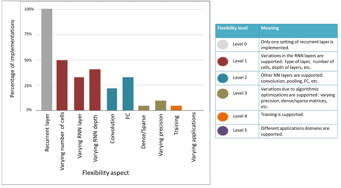
Supporting variations in RNN layers (level 1) Recurrent layers can vary in the type of layers, the number of cells in each layer, and the number of layers (the depth of an RNN model). One optimization that might have a side effect on the flexibility of the solution is the choice of using the on-chip/off-chip memory to store the weights. Being able to store all the weights in the on-chip memory is very beneficial. It leads to better performance and less energy consumption by decreasing the cost of memory accesses. However, the solution may be unfeasible for larger problems. For instance, in F8 [53], the number of weights in the model and their precision are restricted by the on-chip memory size. It is not possible to run a model with an increased number of hidden cells or increased precision. A possible solution is to use an adaptable approach, where the choice of the location of storing the weights is dependent on the model size and thus can support a wide range of models. Another solution was adopted in F12 [15], where part of the weights is stored in the internal memory and the rest is stored in the off-chip memory (Hybrid memory).
Supporting other NN layers (level 2) Supporting other NN layers would allow the solution to run a broader range of NN applications. Nevertheless, other NN layers may exist in the RNN model such as convolutions as a feature extractor. Thus, supporting convolution in the implementation increases the flexibility of the solution, as it can run RNN models with visual inputs and run CNN independent applications.
Supporting algorithmic optimization variations (Level 3) Variations in the optimizations applied are considered as variations in the model as well. For instance, variation due to applying/not applying pruning is the presence of sparse/dense matrices in the matrix to vector multiplications computations. The design in A9 [50] employed a configurable interconnection network topology to increase the flexibility of the accelerator. The accelerator in A9 [50] supported both LSTM and CNN layers. The accelerators supported both sparse and dense matrices. One other variation is the variation in weights and activations precision. The design in A10 [93] supported varying precision models by allowing dynamic precision per layer for both CNN and RNN models. Similarly, Microsoft NPU brainwave architecture [28] supported varying precision using a narrow precision block floating-point format [113].
Online training (Level 4) Incremented online training was supported in A4 [16] to support retraining pre-trained networks to enhance accuracy. Changes in hardware design have been applied to support both training and inference without affecting the quality of inference. For instance, three modes of data transfer were applied. The first is to load new weights. The second is to load input sequences and the third is to update certain weights. Nevertheless, extra precision was used in case of training only. Meeting different applications domains constraints (Level 5) None of the implementations understudy target variations in the application domains constraints. NetAdapt is a good example of an implementation that can adapt to different metric budgets [116]. However, it only targets CNNs.
VI Discussions and opportunities
In the previous section, we studied the implementations of RNN on embedded platforms. Furthermore, in Section II, we have defined the objectives of realizing RNN models on embedded platforms. In this section, we inspect how the objectives are being met by the implementations.
Throughput It is clear that throughput was the main objective for most of the implementations. As seen in Figure 9, high throughput was achieved by many implementations understudy. Algorithmic and memory optimizations are present in most of the high throughput implementations. The algorithmic optimizations applied were effective as they decrease both the computation and memory requirements of the RNN models. For instance, If 4-bit precision is used instead of 32-bit for weights storage, the memory requirement is decreased to . Multiple 4-bit weights can be concatenated during weights fetching. Thus, the number of memory accesses can decrease as well. Furthermore, the hardware required for 4-bit operations is simpler than the hardware required for 32-bit floating-point operations.
Memory specific optimizations are effective because they decrease/hide the overhead of accessing the large number of weights used in RNN computations. Memory access time can be decreased by storing all weights in on-chip memory. However, this can bound the validity of the solution for larger models as on-chip memory may not be enough to store the weights. Overlapping the memory access time with computation and computation in memory are considered as memory optimizations as well.
Energy efficiency
Applying algorithmic and memory access optimizations have a positive effect on energy efficiency as well. The decrease of the number of computations, the complexity of computations, and the number of memory accesses achieved by algorithmic optimizations decrease the amount of energy consumed by the implementation. Nevertheless, minimizing the off-chip memory use by storing weights on on-chip memory enhances the energy efficiency effectually. Analog computing and processing in memory implementations showed superior energy efficiency in ASIC implementations.
Meeting real-time requirements was not used as an objective for many implementations. In a few of the implementations understudy, real-time deadlines were mentioned and followed in the design of the solution.
Flexibilty In Section II-A, flexibility is defined as a secondary objective. Thus, we do not expect flexibility to be fully met by the implementations. Variations in RNN model was partially fulfilled by many implementations. However, the number of variations covered by each implementation is quite low. Few implementations approached other NN layers and variations in algorithmic optimizations. Online-training was targeted by only one implementation. Embedded implementations do not usually support Online-training. While at the algorithmic side, researchers are doing interesting work based on online/continuous training [103, 47]. Supporting different applications was never met by any of the RNN implementations. It has been met by the CNN solution in [116]. Following a similar method in RNNs with addition to supporting models variations can lead to an interesting solution.
Opportunities for future research
Based on the study provided in this article, we list some opportunities for future research.
QRNN and SRU: QRNN and SRU (Section III-B6) are two alternatives to LSTM where the matrix to vector computations at the current time-step are independent on the previous time-step computations. Thus, using them in RNN models can make the parallelization more efficient and consequently lead to better performance.
DeltaRNN [72] and DeltaCNN [14]: We believe that applying the delta algorithm on both recurrent and convolution layers is a logical step due to the temporal relation between the input sequences. Adding delta step to other algorithmic optimizations such as pruning and quantization would decrease the memory access and computation requirements.
Block-circulant matrices Using block-circulant matrices as an algorithmic optimization decreases the RNN size while avoiding irregularity of computation as introduced by pruning [109]. Applying circulant matrices can be accompanied by low precision parameters and activations with a small effect on accuracy [112]. With the addition to applying the delta algorithm as mentioned earlier, RNN inference can achieve a promising throughput and energy efficiency.
Hybrid optimizations: It has been shown that a mix of algorithmic optimizations can be applied to an RNN model with an acceptable loss in accuracy [112]. Applying a mix of optimizations would enable the implementations to benefit from each optimization. For an RNN implementation, three classes of optimizations can be mixed with tuning. The first optimization as mentioned earlier is the delta algorithm and the corresponding parameter is delta. The second is quantization and the corresponding parameters are the number of bits and quantization method. The third optimization is compression. If the applied compression technique is block-circulant matrices, the parameter will be the block size. Tuning the three parameters delta, number of bits, quantization method, and block size, the designer can reach the highest performance while keeping the accuracy within an acceptable range (the range is dependant on the application).
Analog computing and processing in memory: Analog computing [124] and processing in memory [118, 6] have shown promising performance, especially in energy efficiency. Analog crossbar based matrix to vector multiplication units can provide low latency and computing in memory overcomes the memory access problems.
Flexible neural networks domain-specific architectures Domain-specific architectures (DSAs) are pointed out as a future opportunity in the field of computer architecture [44]. DSAs (called accelerators or custom hardware as well) for neural networks applications can reach high performance and energy efficiency. Designing an architecture for neural networks applications as a specific domain with a known memory access patterns enhances the parallelism and the use of memory hierarchy. Nevertheless, it is possible to use less precision and benefit from domain-specific languages (DSLs). Google Edge TPU is an example for a DSA for neural networks inference using 8-bit precision [2]. Based on the study in this article, we add that the neural networks DSA needs to support flexibility. For flexibility aspects defined earlier in Section II to be fulfilled, there are some features need to be supported in the underlying hardware.
- •
Variable bit-width operations as in A10 [93] to support different quantization schemes.
- •
Some optimizations require pre/post-processing on input vectors and weights. Support for weights reordering, delta vectors computation, retaining circulant matrices from equivalent vectors, and other operations required by miscellaneous optimizations would be useful.
- •
Support for training that would imply the support of back-propagation and the allowance of weights modification.
VII Summary
Today we see a trend towards more intelligent mobile devices that are processing applications with stream data in the form of text, voice, and video. To process these applications, RNNs are important due to their efficiency in processing sequential data. In this article, we study the state-of-the-art in RNN implementations from the embedded systems perspective. The article includes all the aspects required for the efficient implementation of an RNN model on embedded platforms. To do so, we study the different components of RNN models from an implementation point of view more than an algorithmic point of view. Nevertheless, we define the objectives that are required to be met by the hardware solutions for RNN applications and the challenges making them difficult. For an RNN model to run efficiently on an embedded platform, some optimizations need to be applied. Thus, we study both algorithmic and platform-specific optimizations. Then, we analyze the implementations of RNN models on embedded systems. Finally, we discuss how the objectives defined earlier in the article have been met and highlight possible directions for research in this field in the future.
We conclude from the analysis of the implementations that there exist two common optimizations for most of the efficient implementations. The first is the algorithmic optimizations. The second is to decrease the memory access time for weights retrieval either by relying on the on-chip memory for storing the weights, applying an efficient overlap between weights loading and computations, or computing in memory. However, using analog crossbar based multipliers can achieve high performance without relying much on algorithmic optimizations. Nevertheless, the study of the implementations in the literature shows enough performance for many streaming applications while showing a lack of flexibility. Finally, we deduce some opportunities for research to fill in the gap between the defined objectives and the research work understudy. We highlight some hardware efficient recurrent layers and algorithmic optimizations that can enhance implementations efficiency. Additionally, we state how can custom embedded hardware implementations support flexible RNNs solutions.
References
- [1] Android RenderScript kernel description. https://developer.android.com/guide/topics/renderscript/compute.html. Accessed: 2019-01-05.
- [2] Google edge TPU. https://cloud.google.com/edge-tpu/. Accessed: 2019-11-5.
- [3] AN4 dataset, 1991 (accessed October 30, 2018). http://www.speech.cs.cmu.edu/databases/an4/.
- [4] WMT’14 dataset, (accessed January 7, 2019). https://nlp.stanford.edu/projects/nmt/.
- [5] Md. Zahangir Alom, Adam T. Moody, Naoya Maruyama, Brian C. Van Essen, and Tarek M. Taha. Effective quantization approaches for recurrent neural networks. CoRR, abs/1802.02615, 2018.
- [6] Aayush Ankit, Izzat El Hajj, Sai Rahul Chalamalasetti, Geoffrey Ndu, Martin Foltin, R. Stanley Williams, Paolo Faraboschi, Wen-Mei Hwu, John Paul Strachan, Kaushik Roy, and Dejan S. Milojicic. PUMA: A programmable ultra-efficient memristor-based accelerator for machine learning inference. CoRR, abs/1901.10351, 2019.
- [7] A. J. Annunziata, M. C. Gaidis, L. Thomas, C. W. Chien, C. C. Hung, P. Chevalier, E. J. O’Sullivan, J. P. Hummel, E. A. Joseph, Y. Zhu, T. Topuria, E. Delenia, P. M. Rice, S. S. P. Parkin, and W. J. Gallagher. Racetrack memory cell array with integrated magnetic tunnel junction readout. In 2011 International Electron Devices Meeting, pages 24.3.1–24.3.4, Dec 2011.
- [8] Yoshua Bengio. Learning deep architectures for ai. Found. Trends Mach. Learn., 2(1):1–127, January 2009.
- [9] Yoshua Bengio, Réjean Ducharme, Pascal Vincent, and Christian Janvin. A neural probabilistic language model. J. Mach. Learn. Res., 3:1137–1155, March 2003.
- [10] K. Bong, S. Choi, C. Kim, S. Kang, Y. Kim, and H. Yoo. 14.6 a 0.62mw ultra-low-power convolutional-neural-network face-recognition processor and a cis integrated with always-on haar-like face detector. In 2017 IEEE International Solid-State Circuits Conference (ISSCC), pages 248–249, Feb 2017.
- [11] Nicolas Boulanger-Lewandowski, Y Bengio, and Pascal Vincent. Modeling temporal dependencies in high-dimensional sequences: Application to polyphonic music generation and transcription. Proceedings of the 29th International Conference on Machine Learning, ICML 2012, 2, 06 2012.
- [12] James Bradbury, Stephen Merity, Caiming Xiong, and Richard Socher. Quasi-recurrent neural networks. CoRR, abs/1611.01576, 2016.
- [13] Qingqing Cao, Niranjan Balasubramanian, and Aruna Balasubramanian. Mobirnn: efficient recurrent neural network execution on mobile GPU. CoRR, abs/1706.00878, 2017.
- [14] Lukas Cavigelli, Philippe Degen, and Luca Benini. Cbinfer: change-based inference for convolutional neural networks on video data. CoRR, abs/1704.04313, 2017.
- [15] A. X. M. Chang and E. Culurciello. Hardware accelerators for recurrent neural networks on fpga. In 2017 IEEE International Symposium on Circuits and Systems (ISCAS), pages 1–4, May 2017.
- [16] C. Chen, H. Ding, H. Peng, H. Zhu, R. Ma, P. Zhang, X. Yan, Y. Wang, M. Wang, H. Min, and R. C. . Shi. Ocean: an on-chip incremental-learning enhanced processor with gated recurrent neural network accelerators. In ESSCIRC 2017 - 43rd IEEE European Solid State Circuits Conference, pages 259–262, Sept 2017.
- [17] Yu-Hsin Chen, Joel Emer, and Vivienne Sze. Eyeriss: a spatial architecture for energy-efficient dataflow for convolutional neural networks. In Proceedings of the 43rd International Symposium on Computer Architecture, ISCA ’16, pages 367–379, Piscataway, NJ, USA, 2016. IEEE Press.
- [18] Yu Cheng, Duo Wang, Pan Zhou, and Tao Zhang. A survey of model compression and acceleration for deep neural networks. CoRR, abs/1710.09282, 2017.
- [19] P. Chi, S. Li, C. Xu, T. Zhang, J. Zhao, Y. Liu, Y. Wang, and Y. Xie. Prime: A novel processing-in-memory architecture for neural network computation in reram-based main memory. In 2016 ACM/IEEE 43rd Annual International Symposium on Computer Architecture (ISCA), pages 27–39, June 2016.
- [20] KyungHyun Cho, Bart van Merrienboer, Dzmitry Bahdanau, and Yoshua Bengio. On the properties of neural machine translation: encoder-decoder approaches. CoRR, abs/1409.1259, 2014.
- [21] Jinil Chung, Jongsun Park, and Swaroop Ghosh. Domain wall memory based convolutional neural networks for bit-width extendability and energy-efficiency. In Proceedings of the 2016 International Symposium on Low Power Electronics and Design, ISLPED ’16, pages 332–337, New York, NY, USA, 2016. ACM.
- [22] Junyoung Chung, Çaglar Gülçehre, KyungHyun Cho, and Yoshua Bengio. Empirical evaluation of gated recurrent neural networks on sequence modeling. CoRR, abs/1412.3555, 2014.
- [23] Matthieu Courbariaux, Yoshua Bengio, and Jean-Pierre David. Binaryconnect: training deep neural networks with binary weights during propagations. CoRR, abs/1511.00363, 2015.
- [24] Xiaoliang Dai, Hongxu Yin, and Niraj K. Jha. Nest: a neural network synthesis tool based on a grow-and-prune paradigm. CoRR, abs/1711.02017, 2017.
- [25] Xiaoliang Dai, Hongxu Yin, and Niraj K. Jha. Grow and prune compact, fast, and accurate lstms. CoRR, abs/1805.11797, 2018.
- [26] Li Deng. A tutorial survey of architectures, algorithms, and applications for deep learning. APSIPA Transactions on Signal and Information Processing, 3:e2, 2014.
- [27] Jeff Donahue, Lisa Anne Hendricks, Sergio Guadarrama, Marcus Rohrbach, Subhashini Venugopalan, Kate Saenko, and Trevor Darrell. Long-term recurrent convolutional networks for visual recognition and description. CoRR, abs/1411.4389, 2014.
- [28] J. Fowers, K. Ovtcharov, M. Papamichael, T. Massengill, M. Liu, D. Lo, S. Alkalay, M. Haselman, L. Adams, M. Ghandi, S. Heil, P. Patel, A. Sapek, G. Weisz, L. Woods, S. Lanka, S. K. Reinhardt, A. M. Caulfield, E. S. Chung, and D. Burger. A configurable cloud-scale dnn processor for real-time ai. In 2018 ACM/IEEE 45th Annual International Symposium on Computer Architecture (ISCA), pages 1–14, June 2018.
- [29] Chang Gao, Daniel Neil, Enea Ceolini, Shih-Chii Liu, and Tobi Delbrück. Deltarnn: a power-efficient recurrent neural network accelerator. In FPGA, 2018.
- [30] John Garofalo, D Graff, D Paul, and D Pallet. Csr-i (wsjo) sennheiser. Linguistic Data Consortium, Philadelphia.
- [31] J. S. Garofolo, L. F. Lamel, W. M. Fisher, J. G. Fiscus, D. S. Pallett, and N. L. Dahlgren. Darpa timit acoustic phonetic continuous speech corpus cdrom, 1993.
- [32] F. A. Gers and J. Schmidhuber. Recurrent nets that time and count. In Proceedings of the IEEE-INNS-ENNS International Joint Conference on Neural Networks. IJCNN 2000. Neural Computing: New Challenges and Perspectives for the New Millennium, volume 3, pages 189–194 vol.3, July 2000.
- [33] J. S. P. Giraldo and M. Verhelst. Laika: a 5uw programmable lstm accelerator for always-on keyword spotting in 65nm cmos. In ESSCIRC 2018 - IEEE 44th European Solid State Circuits Conference (ESSCIRC), pages 166–169, Sept 2018.
- [34] Alex Graves. Generating sequences with recurrent neural networks. CoRR, abs/1308.0850, 2013.
- [35] Alex Graves. Generating sequences with recurrent neural networks. CoRR, abs/1308.0850, 2013.
- [36] Alex Graves, Abdel-rahman Mohamed, and Geoffrey E. Hinton. Speech recognition with deep recurrent neural networks. CoRR, abs/1303.5778, 2013.
- [37] Y. Guan, Z. Yuan, G. Sun, and J. Cong. Fpga-based accelerator for long short-term memory recurrent neural networks. In 2017 22nd Asia and South Pacific Design Automation Conference (ASP-DAC), pages 629–634, Jan 2017.
- [38] Yiwen Guo, Anbang Yao, Hao Zhao, and Yurong Chen. Network sketching: exploiting binary structure in deep CNNs. CoRR, abs/1706.02021, 2017.
- [39] Yunhui Guo. A survey on methods and theories of quantized neural networks, 2018.
- [40] Kartiki Gupta and Divya Gupta. An analysis on lpc, rasta and mfcc techniques in automatic speech recognition system. In 2016 6th International Conference-Cloud System and Big Data Engineering (Confluence), pages 493–497. IEEE, 2016.
- [41] Song Han, Junlong Kang, Huizi Mao, Yiming Hu, Xin Li, Yubin Li, Dongliang Xie, Hong Luo, Song Yao, Yu Wang, Huazhong Yang, and William J. Dally. ESE: efficient speech recognition engine with compressed LSTM on FPGA. CoRR, abs/1612.00694, 2016.
- [42] Song Han, Xingyu Liu, Huizi Mao, Jing Pu, Ardavan Pedram, Mark A. Horowitz, and William J. Dally. EIE: efficient inference engine on compressed deep neural network. CoRR, abs/1602.01528, 2016.
- [43] Song Han, Huizi Mao, and William J. Dally. Deep compression: compressing deep neural network with pruning, trained quantization and huffman coding. CoRR, abs/1510.00149, 2015.
- [44] John L. Hennessy and David A. Patterson. A new golden age for computer architecture. Commun. ACM, 62(2):48–60, January 2019.
- [45] Sepp Hochreiter and Jürgen Schmidhuber. Long short-term memory. Neural Comput., 9(8):1735–1780, November 1997.
- [46] Itay Hubara, Matthieu Courbariaux, Daniel Soudry, Ran El-Yaniv, and Yoshua Bengio. Binarized neural networks. In Proceedings of the 30th International Conference on Neural Information Processing Systems, NIPS’16, pages 4114–4122, USA, 2016. Curran Associates Inc.
- [47] Christoph Käding, Erik Rodner, Alexander Freytag, and Joachim Denzler. Fine-tuning deep neural networks in continuous learning scenarios. In ACCV Workshops, 2016.
- [48] A. Karpathy and L. Fei-Fei. Deep visual-semantic alignments for generating image descriptions. In 2015 IEEE Conference on Computer Vision and Pattern Recognition (CVPR), pages 3128–3137, June 2015.
- [49] Yoon Kim and Alexander M. Rush. Sequence-level knowledge distillation. CoRR, abs/1606.07947, 2016.
- [50] Hyoukjun Kwon, Ananda Samajdar, and Tushar Krishna. Maeri: Enabling flexible dataflow mapping over dnn accelerators via reconfigurable interconnects. SIGPLAN Not., 53(2):461–475, March 2018.
- [51] N. D. Lane, S. Bhattacharya, P. Georgiev, C. Forlivesi, L. Jiao, L. Qendro, and F. Kawsar. Deepx: a software accelerator for low-power deep learning inference on mobile devices. In 2016 15th ACM/IEEE International Conference on Information Processing in Sensor Networks (IPSN), pages 1–12, April 2016.
- [52] Vadim Lebedev, Yaroslav Ganin, Maksim Rakhuba, Ivan Oseledets, and Victor Lempitsky. Speeding-up convolutional neural networks using fine-tuned cp-decomposition. 12 2014.
- [53] Minjae Lee, Kyuyeon Hwang, Jinhwan Park, Sungwook Choi, Sungho Shin, and Wonyong Sung. Fpga-based low-power speech recognition with recurrent neural networks. In Signal Processing Systems (SiPS), 2016 IEEE International Workshop on, pages 230–235. IEEE, 2016.
- [54] Tao Lei, Yu Zhang, and Yoav Artzi. Training RNNs as fast as CNNs. CoRR, abs/1709.02755, 2017.
- [55] R. Leonard. A database for speaker-independent digit recognition. In ICASSP ’84. IEEE International Conference on Acoustics, Speech, and Signal Processing, volume 9, pages 328–331, March 1984.
- [56] Fengfu Li and Bin Liu. Ternary weight networks. CoRR, abs/1605.04711, 2016.
- [57] J. Li and Y. Shen. Image describing based on bidirectional lstm and improved sequence sampling. In 2017 IEEE 2nd International Conference on Big Data Analysis (ICBDA)(, pages 735–739, March 2017.
- [58] Yang Li, Quan Pan, Tao Yang, Suhang Wang, Jiliang Tang, and Erik Cambria. Learning word representations for sentiment analysis. Cognitive Computation, 9(6):843–851, Dec 2017.
- [59] Zhe Li, Caiwen Ding, Siyue Wang, Wujie Wen, Youwei Zhuo, Chang Liu, Qinru Qiu, Wenyao Xu, Xue Lin, Xuehai Qian, and Yanzhi Wang. E-RNN: design optimization for efficient recurrent neural networks in fpgas. CoRR, abs/1812.07106, 2018.
- [60] Tsung-Yi Lin, Michael Maire, Serge J. Belongie, Lubomir D. Bourdev, Ross B. Girshick, James Hays, Pietro Perona, Deva Ramanan, Piotr Dollár, and C. Lawrence Zitnick. Microsoft COCO: common objects in context. CoRR, abs/1405.0312, 2014.
- [61] Zachary Chase Lipton. A critical review of recurrent neural networks for sequence learning. CoRR, abs/1506.00019, 2015.
- [62] Y. Long, T. Na, and S. Mukhopadhyay. Reram-based processing-in-memory architecture for recurrent neural network acceleration. IEEE Transactions on Very Large Scale Integration (VLSI) Systems, 26(12):2781–2794, Dec 2018.
- [63] Y. Long, T. Na, and S. Mukhopadhyay. Reram-based processing-in-memory architecture for recurrent neural network acceleration. IEEE Transactions on Very Large Scale Integration (VLSI) Systems, pages 1–14, 2018.
- [64] Andrew L. Maas, Raymond E. Daly, Peter T. Pham, Dan Huang, Andrew Y. Ng, and Christopher Potts. Learning word vectors for sentiment analysis. In Proceedings of the 49th Annual Meeting of the Association for Computational Linguistics: Human Language Technologies, pages 142–150, Portland, Oregon, USA, June 2011. Association for Computational Linguistics.
- [65] Matt Mahoney. About the test data, 2006 (accessed October 30, 2018). http://mattmahoney.net/dc/textdata.
- [66] D. Maliuk and Y. Makris. An experimentation platform for on-chip integration of analog neural networks: A pathway to trusted and robust analog/rf ics. IEEE Transactions on Neural Networks and Learning Systems, 26(8):1721–1734, Aug 2015.
- [67] Mitchell P. Marcus, Mary Ann Marcinkiewicz, and Beatrice Santorini. Building a large annotated corpus of english: the penn treebank. Comput. Linguist., 19(2):313–330, June 1993.
- [68] Stephen Merity, Caiming Xiong, James Bradbury, and Richard Socher. Pointer sentinel mixture models. CoRR, abs/1609.07843, 2016.
- [69] R. Muscedere, V. Dimitrov, G. A. Jullien, and W. C. Miller. Efficient techniques for binary-to-multidigit multidimensional logarithmic number system conversion using range-addressable look-up tables. IEEE Transactions on Computers, 54(3):257–271, March 2005.
- [70] Sharan Narang, Gregory F. Diamos, Shubho Sengupta, and Erich Elsen. Exploring sparsity in recurrent neural networks. CoRR, abs/1704.05119, 2017.
- [71] Sharan Narang, Eric Undersander, and Gregory Diamos. Block-sparse recurrent neural networks. arXiv preprint arXiv:1711.02782, 2017.
- [72] Daniel Neil, Junhaeng Lee, Tobi Delbrück, and Shih-Chii Liu. Delta networks for optimized recurrent network computation. CoRR, abs/1612.05571, 2016.
- [73] Alexander Novikov, Dmitry Podoprikhin, Anton Osokin, and Dmitry P. Vetrov. Tensorizing neural networks. CoRR, abs/1509.06569, 2015.
- [74] Joachim Ott, Zhouhan Lin, Ying Zhang, Shih-Chii Liu, and Yoshua Bengio. Recurrent neural networks with limited numerical precision. CoRR, abs/1608.06902, 2016.
- [75] V. Panayotov, G. Chen, D. Povey, and S. Khudanpur. Librispeech: an asr corpus based on public domain audio books. In 2015 IEEE International Conference on Acoustics, Speech and Signal Processing (ICASSP), pages 5206–5210, April 2015.
- [76] Bo Pang and Lillian Lee. Opinion mining and sentiment analysis. Found. Trends Inf. Retr., 2(1-2):1–135, January 2008.
- [77] J. Park, J. Kung, W. Yi, and J. J. Kim. Maximizing system performance by balancing computation loads in lstm accelerators. In 2018 Design, Automation Test in Europe Conference Exhibition (DATE), pages 7–12, March 2018.
- [78] Stuart SP Parkin, Masamitsu Hayashi, and Luc Thomas. Magnetic domain-wall racetrack memory. Science, 320(5873):190–194, 2008.
- [79] Razvan Pascanu, Çaglar Gülçehre, Kyunghyun Cho, and Yoshua Bengio. How to construct deep recurrent neural networks. CoRR, abs/1312.6026, 2013.
- [80] F. Piazza, A. Uncini, and M. Zenobi. Neural networks with digital lut activation functions. In Proceedings of 1993 International Conference on Neural Networks (IJCNN-93-Nagoya, Japan), volume 2, pages 1401–1404 vol.2, Oct 1993.
- [81] Jan M. Rabaey. Digital Integrated Circuits: A Design Perspective. Prentice-Hall, Inc., Upper Saddle River, NJ, USA, 1996.
- [82] Mohammad Rastegari, Vicente Ordonez, Joseph Redmon, and Ali Farhadi. Xnor-net: imagenet classification using binary convolutional neural networks. CoRR, abs/1603.05279, 2016.
- [83] Michalis Rizakis, Stylianos I. Venieris, Alexandros Kouris, and Christos-Savvas Bouganis. Approximate fpga-based lstms under computation time constraints. CoRR, abs/1801.02190, 2018.
- [84] Vladimir Rybalkin, Alessandro Pappalardo, Muhammad Mohsin Ghaffar, Giulio Gambardella, Norbert Wehn, and Michaela Blott. Finn-l: library extensions and design trade-off analysis for variable precision lstm networks on fpgas. CoRR, abs/1807.04093, 2018.
- [85] Vladimir Rybalkin, Norbert Wehn, Mohammad Reza Yousefi, and Didier Stricker. Hardware architecture of bidirectional long short-term memory neural network for optical character recognition. In Proceedings of the Conference on Design, Automation & Test in Europe, pages 1394–1399. European Design and Automation Association, 2017.
- [86] Haşim Sak, Andrew Senior, and Françoise Beaufays. Long short-term memory recurrent neural network architectures for large scale acoustic modeling. In Fifteenth annual conference of the international speech communication association, 2014.
- [87] Hojjat Salehinejad, Julianne Baarbe, Sharan Sankar, Joseph Barfett, Errol Colak, and Shahrokh Valaee. Recent advances in recurrent neural networks. CoRR, abs/1801.01078, 2018.
- [88] Mohammad Hossein Samavatian, Anys Bacha, Li Zhou, and Radu Teodorescu. Rnnfast: An accelerator for recurrent neural networks using domain wall memory. CoRR, abs/1812.07609, 2018.
- [89] Eder Santana and George Hotz. Learning a driving simulator. CoRR, abs/1608.01230, 2016.
- [90] Abigail See, Minh-Thang Luong, and Christopher D. Manning. Compression of neural machine translation models via pruning. CoRR, abs/1606.09274, 2016.
- [91] Ervin Sejdić, Igor Djurović, and Jin Jiang. Time–frequency feature representation using energy concentration: An overview of recent advances. Digital signal processing, 19(1):153–183, 2009.
- [92] A. Shafiee, A. Nag, N. Muralimanohar, R. Balasubramonian, J. P. Strachan, M. Hu, R. S. Williams, and V. Srikumar. Isaac: A convolutional neural network accelerator with in-situ analog arithmetic in crossbars. In 2016 ACM/IEEE 43rd Annual International Symposium on Computer Architecture (ISCA), pages 14–26, June 2016.
- [93] Hardik Sharma, Jongse Park, Naveen Suda, Liangzhen Lai, Benson Chau, Joon Kyung Kim, Vikas Chandra, and Hadi Esmaeilzadeh. Bit fusion: Bit-level dynamically composable architecture for accelerating deep neural networks. CoRR, abs/1712.01507, 2017.
- [94] Xingjian Shi, Zhourong Chen, Hao Wang, Dit-Yan Yeung, Wai-Kin Wong, and Wang-chun Woo. Convolutional LSTM network: a machine learning approach for precipitation nowcasting. CoRR, abs/1506.04214, 2015.
- [95] L. Song, X. Qian, H. Li, and Y. Chen. Pipelayer: A pipelined reram-based accelerator for deep learning. In 2017 IEEE International Symposium on High Performance Computer Architecture (HPCA), pages 541–552, Feb 2017.
- [96] Nitish Srivastava, Elman Mansimov, and Ruslan Salakhutdinov. Unsupervised learning of video representations using lstms. CoRR, abs/1502.04681, 2015.
- [97] Aaron Stillmaker and Bevan Baas. Scaling equations for the accurate prediction of cmos device performance from 180nm to 7nm. Integration, 58:74 – 81, 2017.
- [98] Evangelos Stromatias, Daniel Neil, Michael Pfeiffer, Francesco Galluppi, Steve B. Furber, and Shih-Chii Liu. Robustness of spiking deep belief networks to noise and reduced bit precision of neuro-inspired hardware platforms. Frontiers in Neuroscience, 9:222, 2015.
- [99] Z. Sun, Y. Zhu, Y. Zheng, H. Wu, Z. Cao, P. Xiong, J. Hou, T. Huang, and Z. Que. Fpga acceleration of lstm based on data for test flight. In 2018 IEEE International Conference on Smart Cloud (SmartCloud), pages 1–6, Sept 2018.
- [100] Wonyong Sung and Jinhwan Park. Single stream parallelization of recurrent neural networks for low power and fast inference. CoRR, abs/1803.11389, 2018.
- [101] Ilya Sutskever, Oriol Vinyals, and Quoc V. Le. Sequence to sequence learning with neural networks. CoRR, abs/1409.3215, 2014.
- [102] V. Sze, Y. Chen, T. Yang, and J. S. Emer. Efficient processing of deep neural networks: a tutorial and survey. Proceedings of the IEEE, 105(12):2295–2329, Dec 2017.
- [103] A. Teichman and S. Thrun. Practical object recognition in autonomous driving and beyond. In Advanced Robotics and its Social Impacts, pages 35–38, Oct 2011.
- [104] Aditya Srinivas Timmaraju. Sentiment analysis on movie reviews using recursive and recurrent neural network architectures. 2015.
- [105] Andros Tjandra, Sakriani Sakti, and Satoshi Nakamura. Tensor decomposition for compressing recurrent neural network. CoRR, abs/1802.10410, 2018.
- [106] Stylianos I. Venieris, Alexandros Kouris, and Christos-Savvas Bouganis. toolflows for mapping convolutional neural networks on fpgas: a survey and future directions. CoRR, abs/1803.05900, 2018.
- [107] Vedran Vukotic, Christian Raymond, and Guillaume Gravier. A step beyond local observations with a dialog aware bidirectional GRU network for Spoken Language Understanding. In Interspeech, San Francisco, United States, September 2016.
- [108] Erwei Wang, James J. Davis, Ruizhe Zhao, Ho-Cheung Ng, Xinyu Niu, Wayne Luk, Peter Y. K. Cheung, and George A. Constantinides. Deep neural network approximation for custom hardware: Where we’ve been, where we’re going. CoRR, abs/1901.06955, 2019.
- [109] Shuo Wang, Zhe Li, Caiwen Ding, Bo Yuan, Yanzhi Wang, Qinru Qiu, and Yun Liang. C-LSTM: enabling efficient LSTM using structured compression techniques on fpgas. CoRR, abs/1803.06305, 2018.
- [110] Y. Wang, H. Yu, L. Ni, G. Huang, M. Yan, C. Weng, W. Yang, and J. Zhao. An energy-efficient nonvolatile in-memory computing architecture for extreme learning machine by domain-wall nanowire devices. IEEE Transactions on Nanotechnology, 14(6):998–1012, Nov 2015.
- [111] Yu Wang, Shuang Liang, Song Yao, Yi Shan, Song Han, J. Peng, and Hong Luo. Reconfigurable processor for deep learning in autonomous vehicles. 2017.
- [112] Z. Wang, J. Lin, and Z. Wang. Accelerating recurrent neural networks: a memory-efficient approach. IEEE Transactions on Very Large Scale Integration (VLSI) Systems, 25(10):2763–2775, Oct 2017.
- [113] James H. Wilkinson. Rounding Errors in Algebraic Processes. Dover Publications, Inc., New York, NY, USA, 1994.
- [114] Chen Xu, Jianqiang Yao, Zhouchen Lin, Wenwu Ou, Yuanbin Cao, Zhirong Wang, and Hongbin Zha. Alternating multi-bit quantization for recurrent neural networks. CoRR, abs/1802.00150, 2018.
- [115] Yong Xu, Qiuqiang Kong, Qiang Huang, Wenwu Wang, and Mark D Plumbley. Convolutional gated recurrent neural network incorporating spatial features for audio tagging. In 2017 International Joint Conference on Neural Networks (IJCNN), pages 3461–3466. IEEE, 2017.
- [116] Tien-Ju Yang, Andrew G. Howard, Bo Chen, Xiao Zhang, Alec Go, Vivienne Sze, and Hartwig Adam. Netadapt: platform-aware neural network adaptation for mobile applications. CoRR, abs/1804.03230, 2018.
- [117] Shuochao Yao, Yiran Zhao, Aston Zhang, Lu Su, and Tarek Abdelzaher. Deepiot: compressing deep neural network structures for sensing systems with a compressor-critic framework. In Proceedings of the 15th ACM Conference on Embedded Network Sensor Systems, SenSys ’17, pages 4:1–4:14, New York, NY, USA, 2017. ACM.
- [118] S. Yin, X. Sun, S. Yu, J. Seo, and C. Chakrabarti. A parallel rram synaptic array architecture for energy-efficient recurrent neural networks. In 2018 IEEE International Workshop on Signal Processing Systems (SiPS), pages 13–18, Oct 2018.
- [119] Tom Young, Devamanyu Hazarika, Soujanya Poria, and Erik Cambria. Recent trends in deep learning based natural language processing. CoRR, abs/1708.02709, 2017.
- [120] H. Yu, Y. Wang, S. Chen, W. Fei, C. Weng, J. Zhao, and Z. Wei. Energy efficient in-memory machine learning for data intensive image-processing by non-volatile domain-wall memory. In 2014 19th Asia and South Pacific Design Automation Conference (ASP-DAC), pages 191–196, Jan 2014.
- [121] S. Yu, Z. Li, P. Chen, H. Wu, B. Gao, D. Wang, W. Wu, and H. Qian. Binary neural network with 16 mb rram macro chip for classification and online training. In 2016 IEEE International Electron Devices Meeting (IEDM), pages 16.2.1–16.2.4, Dec 2016.
- [122] Chaoyun Zhang, Paul Patras, and Hamed Haddadi. Deep learning in mobile and wireless networking: a survey. CoRR, abs/1803.04311, 2018.
- [123] X. Zhang, X. Liu, A. Ramachandran, C. Zhuge, S. Tang, P. Ouyang, Z. Cheng, K. Rupnow, and D. Chen. High-performance video content recognition with long-term recurrent convolutional network for fpga. In 2017 27th International Conference on Field Programmable Logic and Applications (FPL), pages 1–4, Sept 2017.
- [124] Zhou Zhao, Ashok Srivastava, Lu Peng, and Qing Chen. Long short-term memory network design for analog computing. J. Emerg. Technol. Comput. Syst., 15(1):13:1–13:27, January 2019.
- [125] Shuchang Zhou, Yuzhi Wang, He Wen, Qinyao He, and Yuheng Zou. Balanced quantization: an effective and efficient approach to quantized neural networks. CoRR, abs/1706.07145, 2017.
- [126] M. Zhu and S. Gupta. To prune, or not to prune: exploring the efficacy of pruning for model compression. ArXiv e-prints, October 2017.