Towards Linearization Machine Learning Algorithms

Abstract

This paper is about a machine learning approach based on the multilinear projection of an unknown function (or probability distribution) to be estimated towards a linear (or multilinear) dimensional space E’. The proposal transforms the problem of predicting the target of an observation x into a problem of determining a consensus among the k nearest neighbors of x’s image within the dimensional space E’. The algorithms that concretize it allow both regression and binary classification. Implementations carried out using Scala/Spark and assessed on a dozen LIBSVM datasets have demonstrated improvements in prediction accuracies in comparison with other prediction algorithms implemented within Spark MLLib such as multilayer perceptrons, logistic regression classifiers and random forests.

Introduction

This work focuses on the supervised learning problem: exploitation of historical data for classification (prediction of discrete values) [1] and regression (prediction of continous values) purposes [2].

Several approaches are proposed to solve the supervised learning problem like for instance:

• Linear regression [3] which consists in using an equation such as $Y=W^{t}X$ to predict the output $Y$ that corresponds to an observation $X=(1,x_{1},...,x_{n})$. Vector $W=(w_{0},w_{1},...,w_{n})$ represents the parameters estimated from historical data $(X_{0},Y_{0})$: $W=(X_{0}^{t}X_{0})^{-1}X_{0}^{t}Y_{0}$ (least squares estimate).

• Logistic regression [4] which is widely used to predict a binary response and consists in using an equation such as $p=1/(1+e^{-(W^{t}X)})$ to predict the output $y$ that corresponds to an observation $X=(1,x_{1},...,x_{n})$: here, $y$ is a binary class whose value depends on whether $p>0.5$.

• Random forests [5] which combine separately trained decision trees [6] to improve prediction accuracy. Randomness is injected when training decision trees to reduce the risk of overfitting. Each prediction is obtained through consensus (aka aggregating the results) from the combined decision trees: majority vote in case of classification and averaging in case of regression.

• Multilayer perceptron [7] which consists of several layers of nodes forming a network, each layer being fully connected to the next layer in the network. Nodes in the input layer represent the input data while the other nodes represent linear combinations acting on inputs associated with an activation function. Nodes in the output layer are used to produce the prediction and their number corresponds to the number of classes (number of possible output values).

This paper introduces a novel machine learning approach based on the multilinear projection of an unknown function (or probability distribution) to be estimated towards a linear (or multilinear) dimensional space E’. This transforms the supervised learning problem into a problem of determining a consensus among the k nearest neighbors of image of an input observation x, within the dimensional space E’. The proposal is concretized into algorithms that allow both regression and binary classification. For a multiclass classification, one can consider transformation to binary multi-class classification techniques such as one-against-all [8]. Implementations [9] carried out using Scala/Spark [10, 11] and assessed on a dozen LIBSVM datasets (breast-cancer, a1a, a2a, iris_libsvm, square root function dataset, etc. [12, 13] have demonstrated improvements in prediction accuracies in comparison with Spark MLLib [14] implementations of multilayer perceptrons, logistic regression classifiers and random forests.

In the following, we present the approach, describe the algorithms and discuss the assessments performed.

1 The Linearization Machine Learning Approach

1.1 Overview

Figure 1: Overview of the linearization machine learning approach

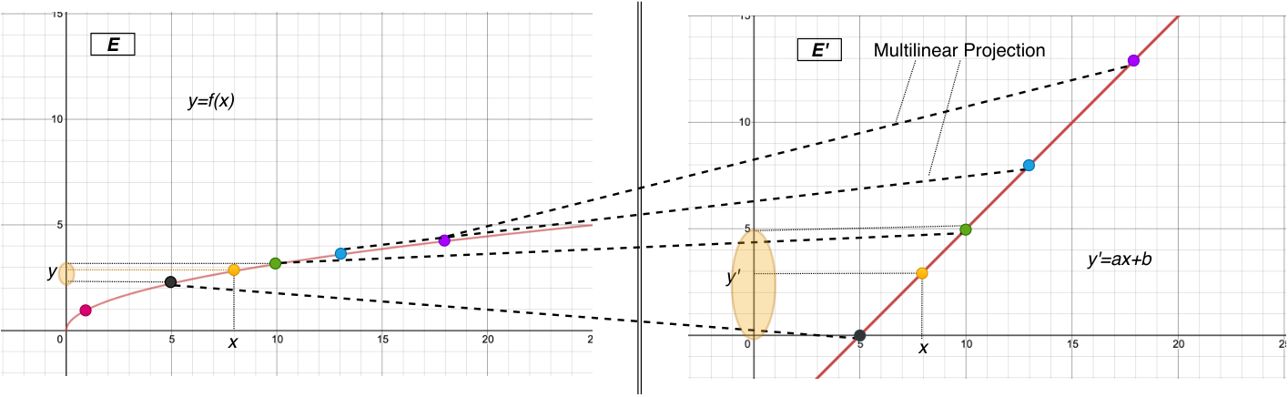
Figure 1 provides an overview of the linearization machine learning approach. Its Scala implementation is available at [9]. An unknown function (or probability distribution) $f(x)$ (respectively $f(X)$ with $X=(1,x_{1},...,x_{n})$) is projected within a space E’ into a linear (respectively multilinear) function $f^{\prime}(x)=ax+b$ (respectively $f^{\prime}(X)=W^{t}X$ with $W=(w_{0},w_{1},...,w_{n})$). The multilinear projection consists of linear transformations of points of the historical dataset (or learning dataset): each linear transformation is defined to map a point $(x_{i},y_{i}=f(x_{i}))$ of $E$ into a point $(x_{i},y^{\prime}_{i}=f^{\prime}(x_{i}))$ of $E^{\prime}$. Coefficients $(a,b)or(w_{0},w_{1},...,w_{n})$ are parameters of the learning model. They must be fine tuned using optimization algorithms.

Let $x$ be a new observation and $(y^{\prime}_{j_{1}},...y^{\prime}_{j_{k}})$ be the k nearest neighbors of $y^{\prime}=f^{\prime}(x)$ following a distance such as the absolute value of the difference ($k\in 1..n$ is also a parameter of the learning model which must be fine tuned). The prediction $y$ is given by:

$$y=\frac{1}{k}{{\sum}}_{t=j_{1}}^{j_{k}}\frac{y^{\prime}*y_{j_{t}}}{y^{\prime}_{j_{t}}}$$

This estimate is obtained by average. The median can also be considered.

1.2 Algorithms

1.2.1 Regression

1. Estimate the best parameter values using an optimization algorithm

2. For an input $X$:

   1. Compute the subset $(y^{\prime}_{j_{1}},...y^{\prime}_{j_{k}})$ of the k nearest neighbors of $y^{\prime}=f^{\prime}(X)$

   2. output $y:=\frac{1}{k}{{\sum}}_{t=j_{1}}^{j_{k}}\frac{y^{\prime}*y_{j_{t}}}{y^{\prime}_{j_{t}}}$

1.2.2 Binary Classification

Let 0 and 1 be the labels and $random$ be a function that allows to randomly choose a value in a given set.

1. For each historical data point $(X_{i},c_{i})$ where $i\in 1..n$:

   1. If $c_{i}=0$, set $p_{i}:=random(]0,0.5[)$

      Else, set $p_{i}:=random(]0.5,1[)$

2. Set $(y_{i})_{i\in 1..n}:=Learn((X_{i})_{i\in 1..n},(c_{i})_{i\in 1..n},(p_{i})_{i\in 1..n})$

3. For an input $x$:

   1. Compute the subset $(y^{\prime}_{j_{1}},...y^{\prime}_{j_{k}})$ of the k nearest neighbors of $y^{\prime}=f^{\prime}(x)$

   2. If $\frac{1}{k}{{\sum}}_{t=j_{1}}^{j_{k}}\frac{y^{\prime}*y_{j_{t}}}{y^{\prime}_{j_{t}}}>0.5$, output 1

      Else, output 0

1.2.3 Function Learn

1. For each historical data point $(X_{i},c_{i})$ where $i\in 1..n$:

   1. Compute the subset $(y^{\prime}_{j_{1}},...y^{\prime}_{j_{k}})$ of the k nearest neighbors of $y^{\prime}_{i}=f^{\prime}(X_{i})$

   2. Set $q_{i}:=\frac{1}{k}{{\sum}}_{t=j_{1}}^{j_{k}}\frac{y^{\prime}_{i}*p_{j_{t}}}{y^{\prime}_{j_{t}}}$

   3. If $|q_{i}-p_{i}|>>0$

      1. If $((c_{i}=0\wedge q_{i}<0.5)\vee(c_{i}=1\wedge q_{i}\in[0.5,1]))$, set $p_{i}:=q_{i}$

         Else if $(q_{i}>>p_{i}\wedge((c_{i}=0\wedge p_{i}+inc<0.5)\vee(c_{i}=1\wedge p_{i}+pas\leq 1)))$ , set $p_{i}:=p_{i}+inc$

         Else if $(q_{i}<<p_{i}\wedge((c_{i}=0\wedge p_{i}-inc\geq 0)\vee(c_{i}=1\wedge p_{i}-inc\geq 0.5)))$, set $p_{i}:=p_{i}-inc$

2. If $(p_{i})_{i\in 1..n}$ has not changed, output $(p_{i})_{i\in 1..n}$

   Else output $Learn((X_{i})_{i\in 1..n},(c_{i})_{i\in 1..n},(p_{i})_{i\in 1..n})$

2 Discussion

The datasets and approach implementations are available at [9]. Our experience, without proper parameter tuning, has been that the linearization machine learning implementations are in many cases more accurate and must be further investigated.

Table 1: Overview of assessment accuracies

Dataset	Multilayer perceptrons	Logistic regression	Linearization ML Approach
breast-cancer	96% (238/248)	86% (213/248)	98% (241/248)
a1a	79% (459/582)	75% (436/582)	74% (425/582)
square root	73% (2560/3507)	57% (1999/3507)	90% (3147/3507)
exp	77% (3087/4010)	77% (3087/4010)	78% (3107/4010)
cod-rna	93% (19463/20929)	66% (13813/20929)	86% (17790/20929)

References

- [1] L. Breiman, Classification and regression trees, Routledge, 2017.
- [2] J. R. Quinlan, et al., Learning with continuous classes, in: 5th Australian joint conference on artificial intelligence, Vol. 92, World Scientific, 1992, pp. 343–348.
- [3] G. A. Seber, A. J. Lee, Linear regression analysis, Vol. 329, John Wiley & Sons, 2012.
- [4] D. G. Kleinbaum, K. Dietz, M. Gail, M. Klein, M. Klein, Logistic regression, Springer, 2002.
- [5] L. Breiman, Random forests, Machine learning 45 (1) (2001) 5–32.
- [6] L. Rokach, O. Z. Maimon, Data mining with decision trees: theory and applications, Vol. 69, World scientific, 2008.
- [7] S. K. Pal, S. Mitra, Multilayer perceptron, fuzzy sets, and classification, IEEE Transactions on neural networks 3 (5) (1992) 683–697.
- [8] C. M. Bishop, Pattern recognition and machine learning, springer, 2006.
- [9]
Scala implementation of