The arithmetic geometry of AdS₂
and its continuum limit

Minos Axenides${}^{(a)},$ Emmanuel Floratos^(a,b) and Stam Nicolis^(c)

^(a) Institute of Nuclear and Particle Physics, NRCPS “Demokritos”
Aghia Paraskevi, GR–15310, Greece

^(b) Physics Department, University of Athens, Zografou University Campus
Athens, GR-15771, Greece

^(c) Institut Denis Poisson, Université de Tours, Université d’Orléans, CNRS (UMR7013)
Parc Grandmont, 37200 Tours, France

We present and study in detail the construction of a discrete and finite arithmetic geometry AdS${}_{2}[N]$ and show that an appropriate scaling limit exists, as $N\to\infty,$ that can be identified with the universal AdS₂ radial and time near horizon geometry of extremal black holes.

The AdS${}_{2}[N]$ geometry has been proposed as a toy model for describing the nonlocal and chaotic dynamics of the horizon microscopic degrees of freedom, that carry the finite black hole entropy. In particular, it supports exact quantum mechanical bulk-boundary holography for single particle wave packet probes, that possess an $N-$dimensional Hilbert space of states.

This costruction amounts, in fact, to a compression of the information about the continuous AdS₂ geometry and it provides an example of a framework for the study of quantum complexity of spacetime geometries.

1 Introduction

At Planck scale energies, quantum mechanics and gravity, together, imply that the notion of spacetime itself becomes ill–defined, through the appearance of black holes, with horizons (and singularities) of Planck length size.

Indeed, the above remarks imply that probably one has to abandon continuity of spacetime, locality of interactions and regularity of dynamics.Indeed there are arguments that quantization of gravity implies discretization of space time [1].

On the other hand, at this point, we would like to ponder about an old question, namely the nature of spacetime at very short distances–of the order of the Planck scale–is that of “continuum” vs. “discretum”. It is argued that, for resolving power of our experiments, much smaller than that of the Planck scale, the continuum description of all physical phenomena on spacetime is perfectly adequate.

As the resolving power increases about the Planck scale, scattering experiments of any sort of particle–like objects will produce, by definition, black holes and the strength of the gravitational interaction will be of O(1), which leads to a breakdown of the usual continuum spacetime description.

In string theory the underlying hypothesis is that spacetime geometry and, thus, gravity, is an emergent phenomenon. This has been shown successfully only for distances much larger than the Planck scale, however, while, at Planck–scale distances, perturbative string theory breaks down and resummation of all string loop scattering amplitudes is, at present, not known [2, 3].

Various efforts, using duality symmetries, between string compactifications at weak and strong coupling, have produced very interesting results in the direction of the unification of all superstring theories to M-theory [4] with the M(atrix) model approach [5, 6], for the moment, the best candidate to represent M-theory.

In the framework of the AdS/CFT correspondence, where unitarity is manifest on both sides, strong coupling–closed–string theory, in the bulk, implies Planck scale curvature for the AdS spacetime(s). In the same limit, the holographically dual conformal field theory (CFT) on the boundary, becomes a free field theory and the problem then boils down to determining infinitely “complicated” operators, in order to represent “local events” in the bulk, as well as the local diffeomorphisms within the bulk, in the language of the boundary theory (the so-called “problem of locality” in the AdS/CFT correspondence–for instance in [7]).

Although the Planck scale energy frontier is very far from any imaginable experimentally accessible scale, there do exist instances in Nature, where the understanding of Planck scale physics becomes imperative. The most important one is the Planck scale spacetime regions at the creation of the Universe (the vicinity of the Big Bang singularity). Although there are interesting theoretical efforts in string theory cosmology [8, 9], they avoid, in essence, addressing the question of the structure of spacetime at sub-Planck scales, by assuming that spacetime doesn’t exist as a fundamental notion at all.

The second instance, where Planck scale physics plays a vital role, is in understanding the near horizon geometry of black holes, as well as the question of quantum mechanical resolution of the (classical) black hole singularity.

In this paper we shall focus on the study of the near horizon geometry of black holes, assuming some general principles, which have emerged during the last forty years.

These principles are:

• Black holes behave like thermodynamic systems, in particular they can be assigned a finite entropy, proportional to the horizon area, which is a universal law for all black holes (the Bekenstein–Christodoulou–Hawking entropy) [10, 11, 12, 13, 14]

• All the information about the “interior” and “exterior” phenomena, with respect to the black hole horizon, is carried by degrees of freedom, that live at a Planck scale “distance” from the horizon (this region is known as the “stretched horizon”). This statement has become known as the “holographic principle” [15, 16, 17, 18].

• The holographic principle implies that there is a finite number of bits of information that can be assigned to any Planck scale area [19, 20].

• The interactions of the horizon degrees of freedom cannot be described by any local field theory and they are strongly chaotic and they exhibit maximal mixing [21, 22, 23].

These general principles have motivated very active research, in order to construct explicit models, that incorporate them, while remaining consistent with the general principles of quantum mechanics, in particular unitarity, thus resolving the old “information paradox”, that was stated by Hawking [24, 25].

The most intense activity, in attempting to resolve the paradox, has taken place in the framework of the AdS/CFT correspondence.

This correspondence consists in constructing a dictionary in order to describe the calculation of physical observables, either in the language of conformal field theory, which lives on the flat boundary of the AdS spacetime, or in the language of gravity, which lives in the bulk [26, 27].

The success of this program has been immense and the hope is that it will be, indeed, the appropriate framework for understanding black hole physics, in full generality [28, 29].

A less intense, but more adventurous, activity is to construct, directly, in the bulk and, in particular, in the vicinity of the black hole horizon, non–local models, that do capture the chaotic and mixing dynamics of the degrees of freedom that reside within Planck scale distance of the horizon as well as deriving general, rigorous, constraints from quantum information theory and entanglement.

In our framework space-time at Planck scales is intrinsically discrete, random (following [1]) and is not emergent from anything else; on the contrary it is from these properties that, at large distances, continuous spacetime geometry can be described as an infrared limit thereof.

This assumption amounts to using appropriate mathematical tools, that can describe the emergence of continuous geometries.

Of paramount importance for the definition of a geometry is its isometry group. This is true, locally, for any known geometry and, globally, for the simplest ones (prominent examples are provided by the spacetimes that are of constant curvature: de Sitter, anti-de Sitter and spheres). For discrete geometries, the relevant mathematical framework is arithmetic geometry, that is, geometries over the rationals ($\mathbb{Q}$), the $p-$adics ($\mathbb{Q}_{p}$) and over finite Galois fields ($\mathrm{Gal}(\mathbb{F}_{p^{n}})$) [30]. The relation between these arithmetic geometries and the continuous ones (over the real, $\mathbb{R},$ or the complex, $\mathbb{C}$ numbers) is the focus of the Langlands program [31].

In our previous work we have proposed a discrete and finite model of the continuous bulk AdS₂ geometry, which we have called AdS${}_{2}[N],$ for any, positive, integer $N.$ This geometry is defined as the set of points of integer entries, $(k,l,m),$ that satisfy the relation $k^{2}+l^{2}-m^{2}\equiv\,1\,\mathrm{mod}\,N.$ Thus, we have replaced, in the definition of the continuous AdS₂ geometry, the real numbers with the integers mod $N.$

AdS${}_{2}[N],$ defined this way, has a random structure, due to the modular arithmetic. As explained in [32, 33, 34], this particular discretization is chosen because it provides a way of constructing a holographic correspondence between the bulk, AdS${}_{2}[N],$ and its boundary, $\mathbb{RP}^{1}[N],$ the discrete projective line.

The reason this discrete holography exists at all is that it is possible to realize the action of the discrete and finite symmetry group of AdS${}_{2}[N],$ which is PSL${}_{2}[N]$: It acts as an isometry group of the bulk and as the (Möbius) conformal group on the boundary.

This geometry provides, also, a natural framework for describing the single particle dynamics, via observers, with time evolution operators that are elements of the isometry group. This is a discrete analog of the superconformal quantum mechanics of probes near the horizon of large extremal black holes [35].

We have studied the quantum mechanics of single particle probes in the AdS${}_{2}[N]$ geometry and we have found that, for observers whose time evolution operator is the Arnol’d cat map, scrambling of, initially Gaussian, wavepackets occurs in a way consistent with the Eigenstate Thermalization Hypothesis and, when the dimension of the Hilbert space takes values in the set of Fibonacci integers, the “fast scrambling bound” [21, 22, 36, 37, 38, 39] is saturated.

In our approach a long–standing question has been the existence of a continuum limit of the finite and random, modular, geometry, AdS${}_{2}[N],$ for $N\to\infty.$ It is easy to see that, using the prime number decomposition $p_{1}^{r_{1}}\cdots p_{n}^{r_{n}}$ of any integer, $N,$ AdS${}_{2}[N]$ factorizes into the factors AdS${}_{2}[p_{1}^{r_{1}}]\times\cdots\times$AdS${}_{2}[p_{n}^{r_{n}}].$

In the present paper we shall demonstrate that the continuous, geometry of AdS₂ emerges from the discrete AdS${}_{2}[N]$ geometry in two steps. The first step involves the discretization of AdS${}_{2},$ using an appropriate spacetime lattice in the embedding 2+1–dimensional, Minkowski, spacetime. This requires introducing an ultraviolet cutoff $a=R_{\mathrm{AdS_{2}}}/M,$ for any integer $M.$ In units of $a,$ $R_{\mathrm{AdS_{2}}}=M.$

The continuum limit is defined by $a\to 0$ and $M\to\infty,$ keeping $R_{\mathrm{AdS_{2}}}$ fixed.

The second step involves the introduction of an infrared cutoff, $L=aN,$ where $N>M,$ such that, in the limit when $M\to\infty$ and $a\to 0$–and $N\to\infty,$ also–$L/R_{\mathrm{AdS_{2}}}\to\mathrm{const}>1.$

The introduction of the infrared cutoff is realized by symmetrically enclosing a region of the throat of the AdS₂ hyperboloid, as large as desired, in a box, of size $L,$ in the embedding spacetime and then imposing periodic boundary conditions.

The lattice, of spacing $a,$ has as symmetries the discrete Lorentz group SO$(2,1,\mathbb{Z})$ and induces, on the continuum AdS${}_{2},$ an infinite set of integral points. This set defines the integral lattice of AdS${}_{2},$ which we shall call henceforth AdS${}_{2}[\mathbb{Z}].$

Obviously, this integral lattice, as a whole, is invariant under the action of SO$(2,1,\mathbb{Z}),$ the discrete Lorentz group in two time and one space-like dimensions [40, 41]. On the other hand, the introduction of the periodic box of size $L=Na$ identifies all the points of the integral lattice, whose coordinates differ by integer multiples of $N.$

This equivalence relation implies that all the integral points of AdS${}_{2},$ which lie outside the box, can be identified with points inside the box, that, however, need not lie on the part of AdS${}_{2},$ that’s enclosed by this box. We observe that the IR cutoff, $N,$ deforms the $SO(2,1,\mathbb{Z})$ symmetry of the integral lattice to its $\mathrm{mod}\,N$ reduction, $SO(2,1,\mathbb{Z}_{N}).$

The images of all points $(k,l,m),$ of AdS${}_{2}[\mathbb{Z}],$ inside this box, satisfy the equation $k^{2}+l^{2}-m^{2}\equiv M^{2}\,\mathrm{mod}\,N.$

In order to identify the solutions of this equation with the elements of AdS${}_{2}[N],$ it is necessary to impose that $M^{2}\equiv\,1\,\mathrm{mod}\,N.$ This conditions provides a relation between the points of AdS${}_{2}[\mathbb{Z}]$ and those of AdS${}_{2}[\mathbb{Z}_{N}],$ as well as an important constraint between the UV and IR cutoffs, $M$ and $N.$

The introduction of the UV and IR cutoffs grant us the possibility of taking the continuum limit of the geometry AdS${}_{2}[N]$ by taking the limit $a\to 0.$ Finally, as we shall show in this paper–and this is our main result–the continuum limit entails finding infinite sequences of UV/IR cutoff pairs $\{(M_{n},N_{n})\},$ where $M_{n}<N_{n}$ for all $n.$ When $n\to\infty,$ $M_{n}$ and $N_{n}$ will tend to infinity in such a way that $0<\lim_{n\to\infty}\,M_{n}/N_{n}=R_{\mathrm{AdS_{2}}}/L\equiv\gamma<1.$

Another result is the explicit construction of such sequences, using properties of generalized $k-$Fibonacci numbers and the ratio $\gamma$ turns out to be the golden $(k=1)$ or, more generally, the “silver” ratios (for $k=2,3,\ldots$). Introducing the $k-$Fibonacci sequence will allow us to remove the IR cutoff, by taking the limit $k\to\infty,$ while keeping $R_{\mathrm{AdS_{2}}}$ fixed.

The plan of our paper is as follows:

In section 2 we, first, recall the salient, standard, features of the geometry of AdS₂ (in 2.1), as a ruling surface and as a coset space; then we introduce the UV cutoff and the integral lattice of AdS₂ as well as its discrete isometry group SO$(2,1,\mathbb{Z}).$ The structure of this discrete Lorentz group is important for the study of hyperbolic algebras [42], since it plays the role of the Weyl group of its root space.

Since the ruling property of the continuous geometry is lost, we provide a detailed construction of the light cone lines, that can contain the integral points. These lines emanate from the rational points of the circle, on the throat of AdS${}_{2}.$ This construction is relevant for understanding the causality structure of this lattice (known as causal diamonds) and for counting the points of this lattice.

Due to the randomness, that is inherent in the factorization of integers, there is a corresponding randomness in the distribution of the lattice points, which is a well known subject in arithmetic geometry [43].

In subsection 2.3 we introduce, also, the IR cutoff, by enclosing (a part of) AdS${}_{2},$ in a symmetric way, within a cube of size $L$ and imposing periodic boundary conditions.

In section 3 we construct the discrete geometry AdS${}_{2}[N],$ by recovering the ruling property, thanks to the mod $N$ operation and we show that the for all of its points there are “precursors” in AdS${}_{2}[\mathbb{Z}].$ This implies that AdS${}_{2}[N]$ is the set of equivalence classes of points of AdS${}_{2}[\mathbb{Z}]$ under the congruent modular group $\Gamma[N].$

Furthermore, we actually count the number of points of the finite geometry AdS${}_{2}[N],$ for every $N$ and we show that, as $N\to\infty,$ this number grows like $N^{2}.$This is important since it demonstrates that almost all of its point are at the boundary allowing the holographic description of the bulk.

In section 4 we study the key equation, $M^{2}\equiv 1\,\mathrm{mod}\,N,$ which we solve, for all $N,$ using the Chinese Remainder Theorem. Furthermore, we use the properties of the Fibonacci sequence, as well as their generalization, the $k-$Fibonacci sequences $(k=1,2,3,\ldots$) to find the infinite sequence of pairs $(M,N),$ that define the correct continuum limit for the infinite folding of the continuous AdS₂ geometry, inside the periodic box.

Finally, we show that the IR cutoff can be removed and obtain the full, infinite, single copy of the continuum AdS₂ geometry, by taking the limit $k\to\infty.$

In section 5 we draw our conclusions and present our ideas for further inquiry.

2 Continuum AdS₂ near horizon BH geometry and the AdS₂ integral lattice

2.1 AdS₂ geometry as a ruling surface and coset space

In this section we review the salient features of the geometry of AdS${}_{2},$ as the single–sheeted hyperboloid, considered as a ruled surface and a coset space [44, 45].

In the near horizon region of spherically symmetric 4d extremal black holes the geometry is known to be of the form AdS${}_{2}\times S^{2},$ where the AdS${}_{2}=SL(2,\mathbb{R})/SO(1,1,\mathbb{R}),$ factor describes the geometry of the radial and time coordinates and $S^{2}$ is the horizon surface.

The AdS₂ spacetime, is a one-sheeted hyperboloid defined through its global embedding in Minkowski spacetime with one space– and two time–like dimensions by the equation [46, 47].

$$x_{0}^{2}+x_{1}^{2}-x_{2}^{2}=R_{\mathrm{AdS}_{2}}^{2}$$ (2.1)

We shall work in units where $R_{\mathrm{AdS}_{2}}=1.$

The boundaries of AdS₂ consist of two time–like disconnected circles, where AdS₂ approaches, asymptotically, the light cone of ${\mathscr{M}}^{1,2},$

$$x_{0}^{2}+x_{1}^{2}-x_{2}^{2}=0$$ (2.2)

AdS₂ can be, also, described as the homogeneous space, $SO(1,2)/SO(1,1).$ This case is special, in that $SO(1,2)$ has a double cover, $SL(2,\mathbb{R}),$ so we have $\mathrm{AdS}_{2}=SL(2,\mathbb{R})/SO(1,1).$

In order to establish our notation and conventions , we proceed with the Weyl construction of the double covering group, $SL(2,\mathbb{R}).$

To every point, $x_{\mu}\in\mathrm{AdS}_{2},$ $\mu=0,1,2,$ we assign the traceless, real, $2\times 2$ matrix

$${\sf M}(x)\equiv\left(\begin{array}[]{cc}x_{0}&x_{1}+x_{2}\\ x_{1}-x_{2}&-x_{0}\end{array}\right)$$ (2.3)

Its determinant is, $\mathrm{det}\,{\sf M}(x)=-x_{0}^{2}-x_{1}^{2}+x_{2}^{2}=-1.$

The action of any element ${\sf A}$ of the isometry group SL$(2,\mathbb{R})$ on AdS₂ is defined through the mapping

$${\sf M}(x^{\prime})={\sf A}{\sf M}(x){\sf A}^{-1}$$ (2.4)

This induces an $SO(1,2)$ transformation on $(x_{0},x_{+},x_{-}),$ where $x_{\pm}=x_{1}\pm x_{2}.$

$$x^{\prime}\equiv\Lambda({\sf A})x$$ (2.5)

More concretely, when

$${\sf A}=\left(\begin{array}[]{cc}a&b\\ c&d\end{array}\right)$$ (2.6)

then the induced Lorentz transform, $\Lambda({\sf A}),$ in the light cone basis $(x_{0},x_{+},x_{-}),$ is given by the expression

$$\Lambda({\sf A})=\left(\begin{array}[]{ccc}ad+bc&-ac&bd\\ -2ab&a^{2}&-b^{2}\\ 2cd&-c^{2}&d^{2}\end{array}\right)$$ (2.7)

Choosing as the origin of coordinates, the base point $\bm{p}\equiv(1,0,0),$ its stability group $SO(1,1),$ is the group of Lorentz transformations in the $x_{0}=0$ plane of ${\mathscr{M}}^{1,2}$ or equivalently, the “scaling” subgroup, ${\sf D},$ of $SL(2,\mathbb{R})$

$${\sf D}\ni{\sf S}(\lambda)\equiv\left(\begin{array}[]{cc}\lambda&0\\ 0&\lambda^{-1}\end{array}\right)$$ (2.8)

for $\lambda\in\mathbb{R}^{\ast}.$

For this choice of the stability point, we define the coset, $h_{\sf A},$ by decomposing ${\sf A}$ as

$${\sf A}=h_{\sf A}{\sf S}(\lambda_{\sf A})$$ (2.9)

Thus, we associate uniquely to every point $x\in\mathrm{AdS}_{2}$ the corresponding coset representative $h_{\sf A}(x).$

We introduce now, the global coordinate system, defined by the straight lines that generate AdS₂ and for which it can be checked easily that they form its complete set of light cones.

Consider the two lines, $\bm{l}_{\pm}(\bm{p}),$ passing through the point $\bm{p}\in{\mathscr{M}}^{1,2},$ orthogonal to the $x_{0}$ axis and at angles $\pm\pi/4$ to the $x_{1}=0$ plane. They are defined by the intersection of AdS₂ and the plane $x_{0}=1$ cf. fig. 1.

The coordinates of any point, $\bm{q}_{+}\in\bm{l}_{+}(\bm{p}),$ $\bm{q}_{-}\in\bm{l}_{-}(\bm{p})$ are given as $(1,\mu_{\pm},\pm\mu_{\pm}),$ $\mu_{\pm}\in\mathbb{R}$ correspondingly.

We can parametrize any point $x_{\mu},$ of AdS${}_{2},$ by the intersection of the local light cone lines, $\bm{l}_{\pm}(x),$ with coordinates $\mu_{\pm}$ and $\phi_{\pm}$ through the relations

$$\begin{array}[]{l}\displaystyle x_{0}=\cos\phi_{\pm}-\mu_{\pm}\sin\phi_{\pm}\\ \displaystyle x_{1}=\sin\phi_{\pm}+\mu_{\pm}\cos\phi_{\pm}\\ \displaystyle x_{2}=\pm\mu_{\pm}\end{array}$$ (2.10)

These can be inverted as follows:

$$\begin{array}[]{ccc}\displaystyle e^{\mathrm{i}\phi_{\pm}}=\frac{x_{0}+\mathrm{i}x_{1}}{1\pm\mathrm{i}x_{2}}&&\displaystyle\mu_{\pm}=\pm x_{2}\end{array}$$ (2.11)

The geometric meaning of the coordinates $\phi$ and $\mu$ is that $\mu$ parametrizes the $x_{2},$ space–like, coordinate and, thus, $\mu_{\pm}\sqrt{2}$ parametrizes the light cone lines $\bm{l}_{\pm}(x).$ The angle $\phi_{\pm}$ is the azimuthal angle of the intersection of $\bm{l}_{\pm}(x)$ with the plane $(x_{0},x_{1}).$ From eq. (2.11), by re-expressing numerator and denominator in polar coordinates, we find

$$\phi=\tau-\sigma$$ (2.12)

where $\tau$ and $\sigma$ are the arguments of the complex numbers $x_{0}+\mathrm{i}x_{1}$ and $1+\mathrm{i}x_{2}.$

The corresponding coset parametrization (group coset motion which brings the origin to the point $x$) is:

$$h(\mu_{\pm},\phi_{\pm})={\sf R}(\phi_{\pm}){\sf T}_{\pm}(\mu_{\pm})$$ (2.13)

where

$${\sf R}(\phi)=\left(\begin{array}[]{cc}\cos\phi/2&-\sin\phi/2\\ \sin\phi/2&\cos\phi/2\end{array}\right)$$ (2.14)

and

$${\sf T}_{+}(\mu)=\left[{\sf T}_{-}(-\mu)\right]^{\mathrm{T}}=\left(\begin{array}[]{cc}1&-\mu\\ 0&1\end{array}\right)$$ (2.15)

It is easy to see also, that ${\sf T}_{\pm}(\mu_{\pm}),$ acting on the base point $X(\bm{p}),$ generate the light cone $l_{\pm}(\bm{p}),$ so we identify these one parameter subgroups with the light cones at $\bm{p}.$

Figure 1: The light cone of AdS₂ at $\bm{p}=(1,0,0).$

In the literature the study of fields on AdS₂ requires an extension, to the universal covering of this spacetime, $\widetilde{\mathrm{AdS}_{2}},$ together with appropriate boundary conditions, in order to avoid closed time–like geodesics and reflection of waves from the boundary. This extension can be parametrized using as time coordinate the azimuthal angle $\tau,$ by extending its range, $(-\pi,\pi)$ to $(-\pi+2\pi k,\pi+2\pi(k+1)),$ $k=\pm 1,\pm 2,\ldots$ and by the space coordinate $\sigma\in(-\pi/2,\pi/2),$ defined in eqs. (2.12). The extension of the range of $\tau$ parametrizes the infinitely–sheeted Riemann surface of the function $\log(\cdot),$ used in deriving eq. (2.12).

These parametrizations induce specific metrics on AdS₂ and $\widetilde{\mathrm{AdS}_{2}},$ namely:

$$ds^{2}=(1+\mu^{2})d\phi^{2}+2d\phi d\mu$$ (2.16)

and

$$ds^{2}=\frac{1}{\cos^{2}\sigma}\left[-d\tau^{2}+d\sigma^{2}\right]$$ (2.17)

The latter metric, with $\tau\equiv\sigma+\phi\in\mathbb{R}$ describes the Einstein strip, that has two disconnected boundaries at $\sigma\equiv\pm\pi/2.$

The Einstein strip is the union of an infinite number of copies of AdS${}_{2}.$ It is interesting to note that the coset structure of AdS₂ can be elevated to $\widetilde{\mathrm{AdS}_{2}}$ by using the universal covering group of $SL(2,\mathbb{R}),$ $\widetilde{SL(2,\mathbb{R})},$ which has been explicitly constructed in ref. [48].

2.2 AdS₂ integral lattice and its discrete Lorentz group SO$(2,1,\mathbb{Z})$

We shall now present and study in detail the the lattice of integral points of AdS${}_{2},$ which we denote henceforth as AdS${}_{2}[\mathbb{Z}],$ along with its isometries. This is the first step towards the modular discretization of AdS${}_{2}.$

As we shall show, this lattice is sufficient for the reconstruction of the continuous AdS₂ spacetime, in an appropriate scaling limit.

In previous work [32, 33, 34] we have embarked on a program to address the question of “continuum” vs. “discretum” for specific toy model geometries, e.g. AdS${}_{2},$ based on the idea that spacetime is not emergent, but that the continuum description of spacetime, as a whole, emerges as an infrared limit of a discrete description of spacetime itself, beyond the Planck scale. This can be expressed as the “fractionalization” of spacetime, beyond the Planck scale, in the spirit of the parton model discussed in ref. [5].

The starting point of our construction is that, for extremal black holes, the entropy is, not, only, finite, but fixed, since they don’t radiate. Therefore the dimension of the Hilbert space of single-particle probes of the black hole microstates is finite–we shall call it $N$ in what follows. We interpret this finite number as describing a discrete number of points in the spatial direction of AdS${}_{2}.$

Now AdS₂ is a continuous spacetime and, before we arrive at such a finite dicretization, we study, in some detail, the problem of describing and counting the integral points on it, i.e. with coordinates $k,l,m\in\mathbb{Z},$ satisfying the constraint

$$k^{2}+l^{2}-m^{2}=1$$ (2.18)

The solution to this problem isn’t known in closed form; in the literature there has been considerable effort in counting the number of solutions, in particular the asymptotics of the density of such points [49, 50, 51, 43]. This problem can be mapped to a problem whose solution is known, namely the Gauss circle problem, that of finding the number $r_{2}(m),$ of solutions to the equation $k^{2}+l^{2}=1+m^{2}.$ This number is determined by factorizing $1+m^{2}$ into its prime factors [49] and counting the number of primes, $p_{i},$ of the form $p_{i}\equiv 1\,\mathrm{mod}\,4$ (this is described in detail in [52]) (p. 285 and following).

This factorization procedure generates a sequence of primes that contains an element of inherent randomness–and it is this property that captures the random distribution of the integral points on AdS₂–this is illustrated in figs. 2.

Figure 2: Integral points on AdS${}_{2}.$

Therefore, from these facts, the number of integral points of the hyperboloid, up to height $m,$ is given by the expression

$$\mathrm{Sol}(m)=4+2\sum_{j=1}^{m}r_{2}(j)$$ (2.19)

We plot this function–in a log–log plot–in fig. 3, when $m$ runs from $-200$ to 200.

Figure 3: The number of integral points, on AdS${}_{2},$ as a function of the height, $m,$ in log–log coordinates. Due to symmetry, $m\leftrightarrow-m,$ we plot only the positive values of $m.$

It is, indeed, striking that the result is a straight line (up to, probably, logarithmic corrections).

We shall now discuss how to actually construct these points, using the property that they belong to light–cone lines, which emerge from the rational points of the circle on the throat of AdS${}_{2}.$

For, using the ruling property of AdS${}_{2},$ viz.

$$\begin{array}[]{l}k=\cos\phi-\mu\sin\phi\\ l=\sin\phi+\mu\cos\phi\\ m=\mu\end{array}$$ (2.20)

we may repackage these as follows

$$x_{0}+\mathrm{i}x_{1}=k+\mathrm{i}l=e^{\mathrm{i}\phi}(1+\mathrm{i}\mu)=e^{\mathrm{i}\phi}(1+\mathrm{i}m)\Leftrightarrow e^{\mathrm{i}\phi}=\frac{k+\mathrm{i}l}{1+\mathrm{i}m}$$ (2.21)

hence

$$\begin{array}[]{lll}\displaystyle\cos\phi=\frac{k+lm}{1+m^{2}}&\mathrm{and}&\displaystyle\sin\phi=\frac{l-mk}{1+m^{2}}\end{array}$$ (2.22)

We remark that these are rational numbers–therefore they label rational points on the circle [53].

The light cone lines at $(k,l,m)$ are, therefore, parametrized as

$$\begin{array}[]{l}x_{0}=\frac{k+lm}{1+m^{2}}-\mu\frac{l-mk}{1+m^{2}}\\ x_{1}=\frac{l-mk}{1+m^{2}}+\mu\frac{k+lm}{1+m^{2}}\\ x_{2}=\mu\end{array}$$ (2.23)

(When $\mu=x_{2}=m,$ $x_{0}=k$ and $x_{1}=l.$)

On these specific light-cone lines we shall show that there exist infinitely many integral points, when $\mu,$ that labels the space–like direction $x_{2},$ takes integer values.

Proof.

We write

$$x_{0}(\mu)+\mathrm{i}x_{1}(\mu)=e^{\mathrm{i}\phi}(1+\mathrm{i}\mu)$$ (2.24)

where $\phi$ is defined by eq. (2.22).

If $\mu=n\in\mathbb{Z},$ we would like to show that $x_{0}(n)$ and $x_{1}(n)$ are, also, integers.

This implies that

$$x_{0}(n)+\mathrm{i}x_{1}(n)=\frac{k+\mathrm{i}l}{1+\mathrm{i}m}(1+\mathrm{i}n)$$ (2.25)

should be a Gaussian integer, i.e. $(1+\mathrm{i}m)/(1+\mathrm{i}n)=a+\mathrm{i}b$ with $a,b\in\mathbb{Z}.$

Therefore

$$1+\mathrm{i}n=(a-mb)+\mathrm{i}(am+b)\Leftrightarrow\left\{\begin{array}[]{l}1=a-mb\\ n=am+b\end{array}\right.$$ (2.26)

These expressions imply, in turn, that

$$\begin{array}[]{l}\displaystyle x_{0}=k+b(km-l)\\ \displaystyle x_{1}=l+b(k+lm)\\ \displaystyle x_{2}=n=m+b(1+m^{2})\end{array}$$ (2.27)

This completes the dictionary between the rational points on the circle and the integral points on AdS${}_{2}.$ In these expressions $b$ can take any integer value. ∎

Conversely, any rational point on the unit circle,

$$e^{\mathrm{i}\phi}\equiv\frac{a+\mathrm{i}b}{a-\mathrm{i}b}\Leftrightarrow x_{0}+\mathrm{i}x_{1}=\frac{a+\mathrm{i}b}{a-\mathrm{i}b}(1+\mathrm{i}n)$$ (2.28)

with $a,b\in\mathbb{Z},$ to obtain an integral point, for $\mu=n,$ we must have

$$\frac{1+\mathrm{i}n}{a-\mathrm{i}b}=d+\mathrm{i}c$$ (2.29)

with $c,d\in\mathbb{Z}$

We immediately deduce that

$$\begin{array}[]{l}\displaystyle 1=ad-bc\\ \displaystyle n=ac+bd\\ \end{array}$$ (2.30)

These expressions imply that, given the integers $a$ and $b,$ it’s possible to find the integers $c$ and $d$ and to express the coordinates $x_{0},x_{1}$ and $x_{2}$ as

$$\begin{array}[]{l}\displaystyle x_{0}=ad+bc\\ \displaystyle x_{1}=ac-bd\\ \displaystyle x_{2}=ac+bd\end{array}$$ (2.31)

The Diophantine equation $1=ad-bc$ is solved for $c$ and $d,$ given two coprime integers $a$ and $b,$ by the Euclidian algorithm–which seems to lead to a unique solution, implying that the point $(x_{0},x_{1},x_{2})$ is unique.

However there’s a subtlety! There are infinitely many solutions $(c,d),$ to the equation $ad-bc=1$! The reason is that, given any one solution $(c,d),$ the pair $(c+\kappa a,d+\kappa b),$ with $\kappa\in\mathbb{Z},$ is, also, a solution, as can be checked by substitution.

Therefore there is a one–parameter family of points, labeled by the integer $\kappa$:

$$\begin{array}[]{l}\displaystyle x_{0}=ad+bc+2\kappa ab\\ \displaystyle x_{1}=ac-bd+\kappa(a^{2}-b^{2})\\ \displaystyle x_{2}=ac+bd+\kappa(a^{2}+b^{2})\end{array}$$ (2.32)

We remark, however, that the vector $(2ab,a^{2}-b^{2},a^{2}+b^{2})$ is light–like, with respect to the $(++-)$ metric: $(2ab)^{2}+(a^{2}-b^{2})^{2}-(a^{2}+b^{2})^{2}=0.$ So eq. (2.32) describes a shift of the, original, point $(ad+bc,ac-bd,ac+bd),$ along a light–like direction; and since the shift is linear in the “affine parameter”, $\kappa,$ this generates a light–like line, passing through the original point.

In this way we have established the dictionary between the rational points of the circle and the integral points of the hyperboloid.

Now we proceed with the study of the discrete symmetries of the integral, $\mathscr{M}^{2,1},$ Lorentzian lattice, where the lattice of integral points on AdS₂ is embedded. $\mathscr{M}^{2,1},$ with one space-like and two time-like dimensions, carries as isometry group the group of integral Lorentz boosts SO$(2,1,\mathbb{Z}),$ as well as integral Poincaré translations. The double cover of this infinite and discrete group is SL$(2,\mathbb{Z}),$ the modular group. This has been shown by Schild [40, 41] in the 1940s. The group SO$(2,1,\mathbb{Z})$ can be generated by reflections, as has been shown by Coxeter [54], followed by Vinberg [55] and, finally, by Kac in his famous book [42], where he introduced the notion of hyperbolic, infinite dimensional, Lie algebras. The characteristic property of such algebras is that the discrete Weyl group of their root space is an integral Lorentz group. Generalization from $SL(2,\mathbb{Z})$ to other normed algebras has been studied in [56].

The fundamental domain of SO$(2,1,\mathbb{Z})$ is the minimum set of points of the integral lattice of $\mathscr{M}^{2,1},$which are not related by any element of the group and from which, all the other points of the lattice can be generated by repeated action of the elements of the group. It turns out that the fundamental region is an infinite set of points and can be generated by repeated action of reflections in the following way:

Using the metric $h\equiv\mathrm{diag}(1,1,-1)$ on $\mathscr{M}^{2,1}$ the generating reflections, elements of SO$(2,1,\mathbb{Z}),$ are given by the matrices

$$\begin{array}[]{lclcl}R_{1}=\left(\begin{array}[]{ccc}-1&&\\ &1&\\ &&1\end{array}\right),&&R_{2}=\left(\begin{array}[]{ccc}1&&\\ &1&\\ &&-1\end{array}\right),&&R_{3}=\left(\begin{array}[]{ccc}0&1&\\ 1&0&\\ &&1\end{array}\right)\\ &&R_{4}=\left(\begin{array}[]{ccc}1&-2&-2\\ 2&-1&-2\\ -2&2&3\end{array}\right)\end{array}$$ (2.33)

If $(k,l,m)$ are the coordinates of the integral lattice, the fundamental domain of SO$(2,1,\mathbb{Z})$ can be defined by the conditions $m\geq k+l\geq 0$ and $k\geq l\geq 0.$ This fundamental domain, restricted on AdS${}_{2}[\mathbb{Z}],$ defines the corresponding fundamental domain of SO$(2,1,\mathbb{Z}),$ acting on AdS${}_{2}[\mathbb{Z}].$ This region of AdS${}_{2}[\mathbb{Z}]$ lies in the positive octant of $\mathscr{M}^{2,1}$ and between the two planes, that define the conditions–cf.fig. 4. It is of infinite extent.

Figure 4: The fundamental domain of SO$(2,1,\mathbb{Z})$ on AdS${}_{2}[\mathbb{Z}]$ is the dark green part of the hyperoboloid, in the positive octant, that lies between the two planes, $m\geq k+l\geq 0$ and $k\geq l\geq 0.$

2.3 UV/IR cutoff of AdS₂

Having introduced the lattice of integral points on AdS${}_{2},$ which we consider as defining a UV cutoff, we proceed, now, to impose an infrared (IR) cutoff. The crucial reason for such a cutoff is the interpretation of AdS₂ as a phase space of single particles, due to the symplectic nature of the isometry $SL(2,\mathbb{R})=Sp(2,\mathbb{R})$ and the requirement to realize chaotic and mixing dynamics for geodesic infalling observers (fast scrambling) [32].

Finiteness of the volume in phase space is a necessary condition for mixing (for a detailed discussion of this point cf. [57]).

Having embedded the AdS₂ hyperboloid,

$$x_{0}^{2}+x_{1}^{2}-x_{2}^{2}=R_{\mathrm{AdS}_{2}}^{2}$$ (2.34)

in $\mathscr{M}^{2,1},$ the IR cutoff, $L$ is defined by periodically identifying all the spacetime points of $\mathscr{M}^{2,1},$ if the difference of their coordinates is an integral vector$\times L$:

$$x\sim y\Leftrightarrow x-y=(k,l,m)L$$ (2.35)

where $k,l,m\in\mathbb{Z}.$ In this way we have compactified $\mathscr{M}^{2,1}$ to the three-dimensional torus, of size $L,$ $\mathbb{T}^{3}(L).$

More concretely, $\mathbb{T}^{3}(L)$ is the fundamental domain of the group of integral translations, $\mathbb{Z}\times\mathbb{Z}\times\mathbb{Z},$ acting on $\mathscr{M}^{2,1}.$ To describe this geometric property by the algebraic operation, mod $L,$ that acts on the coordinates of $\mathscr{M}^{2,1},$ we are led to identify the fundamental domain with the positive octant of $\mathscr{M}^{2,1},$ i.e. $x_{0},x_{1},x_{2}\geq 0$

After this compactification, the spacetime geometry of AdS₂ becomes a foliation of the 3-torus, with leaves the images of AdS₂ under the operation mod $L.$ So the equation, whose solutions define the points of the compactified AdS${}_{2},$ is

$$x_{0}^{2}+x_{1}^{2}-x_{2}^{2}\equiv\,R_{\mathrm{AdS_{2}}}^{2}\,\mathrm{mod}\,L$$ (2.36)

where $(x_{0},x_{1},x_{2})\in\mathbb{T}^{3}(L).$

It is obvious, that inside the 3-torus, there is a part of the AdS₂ surface, which corresponds to solutions of eq. (2.36), without the mod $L$ operation. On the other hand, the infinite part of AdS${}_{2},$ that lies outside the torus, is partitioned in infinitely many pieces, which belong to images of $\mathbb{T}^{3}(L)$ in $\mathscr{M}^{2,1},$ which, by the mod $L$ operation are brought inside the torus.

It is illuminating, for visualizing this complex foliation of the 3–torus into AdS₂ pieces, to consider the effect of the periodic compactification on the construction of AdS₂ by the rotation of light cone lines around the circle, which is the throat of AdS${}_{2},$ in the $(x_{0},x_{1})$ plane. This is the ruling mechanism, which was described in the previous subsection.This is displayed in fig. 5.

Figure 5: Rotating lines that rule AdS${}_{2}.$

It is easy to observe, for the initial position of the light cone line $\bm{l}_{+}(\bm{p})$ the mod $L$ operation generates copies of the parts of the (infinite) line outside the 3-torus, which are parallel and coplanar with the part of the line, which lies inside the torus, cf. fig. 6.

Figure 6: Light cone lines in the periodic box.

This happens for every position of the light cone line, after rotation around the throat of AdS${}_{2}.$

Let us provide an explicit construction.

From the equations

$$\begin{array}[]{l}\displaystyle x_{0}=\cos\phi-\mu\sin\phi\\ \displaystyle x_{1}=\sin\phi+\mu\cos\phi\\ \displaystyle x_{2}=\mu\end{array}$$ (2.37)

where $\phi\in[0,2\pi)$ labels the point on the throat and $\mu$ the height along the space-like direction, $x_{2},$ we observe that, for fixed value of $\phi$ the light cone line, passing through any such point, is given, in parametric form by these equations.

For any fixed value of $\phi,$ such that $\cos\phi=p/r$ and $\sin\phi=q/r,$ where $p,q,r$ are integers, with $(p,r)=1=(q,r)$ and $p^{2}+q^{2}=r^{2},$ then, as $\mu$ takes values from $-\infty$ to $+\infty,$

$$\begin{array}[]{l}\displaystyle x_{0}=\frac{p}{r}-\mu\frac{q}{r}\\ \displaystyle x_{1}=\frac{q}{r}+\mu\frac{p}{r}\\ \displaystyle x_{2}=\mu\end{array}$$ (2.38)

we split the range of $\mu$ into segments of length $L,$ which is, not only, the size of the box, but, in particular, its height, along the space-like direction $x_{2}.$ Therefore, $\mu=kL+\nu,$ where $k$ integer, and $0\leq\nu<L.$

We observe that, when $k=nr,$ with $n$ integer, then eqs. (2.38) take the form

$$\left.\begin{array}[]{l}\displaystyle x_{0}\equiv\left(-nqL+\frac{p}{r}\right)-\nu\frac{q}{r}\\ \displaystyle x_{1}\equiv\left(npL+\frac{q}{r}\right)+\nu\frac{p}{r}\\ \displaystyle x_{2}\equiv nrL+\nu\end{array}\right\}\,\mod\,L=\begin{array}[]{l}\displaystyle x_{0}=\frac{p}{r}-\nu\frac{q}{r}\\ \displaystyle x_{1}=\frac{q}{r}+\nu\frac{p}{r}\\ \displaystyle x_{2}=\nu\end{array}$$ (2.39)

But the segment, described by the second set of equations, is identical to that when $k=0$ and the number of parallel segments is $r,$ that sets the period of the splitting of the line, as it extends beyond the cube.

Upon rotating all the line segments inside the cube, around the throat, we generate all the leaves of the image of AdS₂ under the mod $L$ operation. However, as $\phi,$ then takes values, for which $\cos\phi$ or $\sin\phi$ aren’t both rational, this implies that the number of segments, inside the cube, is infinite and, indeed, densely fills the cube. This illustrates a generalization of the well–known torus case, where a line with rational slope is folded in a periodic way inside the torus; otherwise, it covers the torus densely [57].

The next step for defining and elucidating the modular discretization, AdS${}_{2}[N],$ of AdS${}_{2},$ entails introducing a UV cutoff, which will reproduce the lattice of integral points of AdS₂ constructed in the previous subsection.

The physical lengthscale in our problem is the radius of the AdS₂ spacetime, $R_{\mathrm{AdS}_{2}}.$ We set $R_{\mathrm{AdS}_{2}}=1$ and we divide it into $M$ segments, of length $a=R_{\mathrm{AdS}_{2}}/M.$ This defines $a$ as the UV cutoff (lattice spacing) and $M\in\mathbb{N}$ and, hence, a lattice in $\mathscr{M}^{2,1}.$

The continuum limit is defined by taking $M\to\infty$ and $a\to 0$ with $R_{\mathrm{AdS}_{2}}=1$ fixed.

The global, embedding, coordinates $(x_{0},x_{1},x_{2})$ of this lattice are $(ka,la,ma)=a(k,l,m),$ where $k,l,m\in\mathbb{Z},$ so are measured in units of the spacing $a.$ Therefore the lattice points, that lie on AdS₂ satisfy the equation

$$k^{2}+l^{2}-m^{2}=M^{2}$$ (2.40)

whose solutions define AdS${}_{2}[\mathbb{Z}],$ the set of all integral points of AdS${}_{2}[Z],$ with integer radius $M.$

Now we choose the IR cutoff $L$ in units of $a,$ so that $L=aN,$ where $N$ is an integer, independent of $M.$ It is constrained by $N>M,$ since the cube should contain, at least, the throat of AdS${}_{2}.$

So the scaling limit will be to take $M\to\infty,$ $N\to\infty,$ but keeping $L,$ also, fixed.

The periodic nature of the IR cutoff implies that, finally, we must take the images of all integral points of AdS${}_{2}[\mathbb{Z}]$ under the mod $N$ operation, inside the cubic lattice of $N^{3}$ points.

The set of these images satisfy the equations

$$k^{2}+l^{2}-m^{2}\equiv M^{2}\,\mathrm{mod}\,N$$ (2.41)

Our definition for AdS${}_{2}[N]$ in our previous work was similar to the one given here, the only difference being that the RHS of eq. (2.41) was $1\,\mathrm{mod}\,N,$ which was chosen for convenience, not for any intrinsic reason. We remark that the two definitions are consistent iff $M^{2}\equiv\,1\,\mathrm{mod}\,N.$

The solutions of eq. (2.41), when $M^{2}\equiv 1\,\mathrm{mod}\,N,$ define AdS${}_{2}[N].$ This is a random set of points, thereby defining a random geometry, through the mod $N$ operation.

For fixed lattice spacing $a$ and large $N,$ this random set defines a limiting distribution on $\mathscr{M}^{2,1}$ and, as we shall see later, the number of points of AdS${}_{2}[N]$ grows as $N^{2}.$ This implies that “most” of its points are close to the boundary.

3 Reduction mod $N$ of the AdS₂ integral lattice

3.1 The discrete modular geometry AdS${}_{2}[N]$ and its precursors

In this section we describe, in detail, the properties of the random set of points, that constitute AdS${}_{2}[N],$ defined previously.

All the points of AdS${}_{2}[N]$ live inside the cube, of side $L=Na.$ Some of them are integral points of AdS${}_{2}.$ The rest are the mod $N$ reduction of integral points of AdS${}_{2},$ outside the cube cf. fig.7.

Figure 7: The integral points, $(k,l,m),$ that satisfy $k^{2}+l^{2}-m^{2}\equiv 1\,\mathrm{mod}\,47,$ i.e. that belong to AdS${}_{2}[47].$

Although, in the continuum, AdS₂ is generated by the rotation of a light cone line around the circle of the throat, for the integral points this isn’t true. Rather, as shown in the previous section, we can identify a set of light cone lines, emerging from the rational points of this circle, on which all the integral points lie.

This means that a globally defined ruling parametrization of the integral points doesn’t exist.

It is interesting to notice, though, that, for the mod $N$ reduction of AdS${}_{2}[\mathbb{Z}],$ i.e. AdS${}_{2}[N],$ it is possible to define such a global ruling parametrization for $N=p^{r},$ where $p$ is a prime of the form (a) $p\equiv\,3\,\mathrm{mod}\,4,$ while when (b) $p\equiv\,1\,\mathrm{mod}\,4,$ we need two charts to obtain all such points.

Below we shall make this construction explicit.

We, therefore, start, by parametrizing the points of AdS${}_{2}[N]$ by the ruling of the discrete line $\bm{l}=(1,\mu,\mu)$ around the discrete circle of the throat of AdS${}_{2}[N]$:

$$\begin{array}[]{l}x_{0}=a-\mu b\\ x_{1}=b+\mu a\\ x_{2}=\mu\end{array}$$ (3.1)

where $a,b,\mu\in\mathbb{Z}_{N}$ and $a^{2}+b^{2}\equiv\,1\,\mathrm{mod}\,N.$

This parametrization suffices to generate all the points, for case (a), as an explicit comparison with direct counting confirms; for case (b), we must add a second parametrization, by exchanging $x_{0}$ and $x_{1}.$ The reason this is necessary is that, in case (b), given $x_{0}$ and $x_{1}$ it’s not possible to obtain $a$ and $b,$ since there exists a $\mu=\mu_{0},$ such that $\mu_{0}^{2}\equiv-1\,\mathrm{mod}\,N$ in this case.

When $N=p_{1}^{r_{1}}\times\cdots\times p_{k}^{r_{k}},$ we can use the factorization properties of AdS${}_{2}[N]$ and choose the appropriate system of charts to generate the points for each factor separately.

Having described AdS${}_{2}[N],$ we shall now show how it’s related with AdS${}_{2}[\mathbb{Z}].$

Indeed, we shall show that the two categories of points of AdS${}_{2}[N]$–those that belong, also, to AdS${}_{2}[\mathbb{Z}]$ and those that don’t–originate, both, from points of AdS${}_{2}[\mathbb{Z}],$ by the mod $N$ operation.

To do that it is crucial to use the ruling parametrization (3.1). We shall call the points of AdS${}_{2}[\mathbb{Z}]$ the “precursors” of AdS${}_{2}[N].$

Given any point

$$Y=\left(\begin{array}[]{cc}k&l+m\\ l-m&-k\end{array}\right)$$ (3.2)

of AdS${}_{2}[\mathbb{Z}],$ which is a precursor of a point $X$ of AdS${}_{2}[N],$ by acting with elements $\gamma$ of the principal congruence subgroup $\Gamma(N),$ as $Y\to\gamma Y\gamma^{-1},$ we find all the precursors of $X$–and their number is infinite, since $\Gamma(N)$ is an infinite group. This implies that AdS${}_{2}[N]$ is a set of representatives for the equivalence relation on AdS${}_{2}[\mathbb{Z}],$ defined by $\Gamma(N).$

The $\Gamma(N)$ “arithmetic” subgroup of $SL_{2}(\mathbb{Z}),$ called the principal congruent subgroup, has certain arithmetic properties derived from its definition:

$$\Gamma(N)=\left\{\left.\left(\begin{array}[]{cc}1+\kappa N&\lambda N\\ \rho N&1+\sigma N\end{array}\right)\equiv\left(\begin{array}[]{cc}1&0\\ 0&1\end{array}\right)\,\mathrm{mod}\,N\right|\kappa,\lambda,\rho,\sigma\in\mathbb{Z}\right\}$$ (3.3)

namely, $\Gamma(N_{1})\subset\Gamma(N_{2})$ if $N_{1}|N_{2}.$ So it suffices to let $N$ take as values all the different powers of primes.

The way to determine explicitly the precursors of AdS${}_{2}[N]$ is simplified if we consider the precursors of the light cone lines $\bm{l}_{\pm}=(1,\mu,\pm\mu),$ and, independently, the precursors of the points of the throat of AdS${}_{2}[N],$ i.e. $x_{2}=0.$

The precursors of the lines $\bm{l}_{\pm}$ are the integral points of the generating light cones of AdS${}_{2}.$ In group theoretical terms we have to find the precursor of group element

$$T(\mu)=\left(\begin{array}[]{cc}1&1\\ 0&1\end{array}\right)^{\mu}=\left(\begin{array}[]{cc}1&\mu\\ 0&1\end{array}\right)$$ (3.4)

in $SL(2,\mathbb{Z}_{N}).$

This precursor in SL${}_{2}(\mathbb{Z})$ is defined by

$$p(T(\nu))=\left(\begin{array}[]{cc}1&\nu\\ 0&1\end{array}\right)$$ (3.5)

where $\nu\in\mathbb{Z}$ and where $\mu\equiv\nu\,\mathrm{mod}\,N.$

The precursors of the discrete circle $\mathscr{C}_{N}=\{(a,b)|a^{2}+b^{2}\equiv 1\,\mathrm{mod}\,N\}$ are determined as follows: The points of this discrete circle are in 1-to-1 correspondence with the elements of the abelian group

$$SO_{2}(N)=\left\{\left.\left(\begin{array}[]{cc}a&-b\\ b&a\end{array}\right)\right|\,a^{2}+b^{2}\equiv\,1\,\mathrm{mod}\,N\right\}$$ (3.6)

It is possible to show that there exist elements of SL${}_{2}(\mathbb{Z}),$ whose mod $N$ reduction generate SO${}_{2}(N).$ These elements define an, infinite, abelian, subgroup of SL${}_{2}(\mathbb{Z}).$

We work out in detail below the construction of these precursors in the case where $N$ is prime, $p$ (and this can be straightforwardly generalized to powers of odd primes). In this case the group SO${}_{2}(p)$ is cyclic and its generator has been found, for the first 2000 primes, of the form $p=4k-1,$ by random search [58]. It suffices, therefore, to find the precursors of the generator.

For primes $p=4k+1,$ the generator is the diagonal element of SL${}_{2}(\mathbb{Z}_{N})$ corresponding to the primitive element of $\mathbb{Z}_{N}.$

For any $p$ prime of the form $4k-1,$ we choose the corresponding generator $R_{0},$ corresponding to $(a_{0},b_{0}),$ and we find a precursor in SL${}_{2}(\mathbb{Z}).$ The precursors of all other elements of SO${}_{2}(p)$ are powers of this element.

If $(a_{0},b_{0})$ are relative primes, then, by the Euclidian algorithm, there exist two, unique, integers $c_{0}$ and $d_{0}$ such that $a_{0}d_{0}-b_{0}c_{0}=1.$

Thus, a precursor of $R_{0}$ in SL${}_{2}(\mathbb{Z}),$ is the element

$$p(R_{0})\equiv\left(\begin{array}[]{cc}a_{0}&c_{0}\\ b_{0}&d_{0}\end{array}\right)$$ (3.7)

If $(a_{0},b_{0})$ aren’t relative primes, then we replace the previous element by

$$p(R_{0})\equiv\left(\begin{array}[]{cc}a_{0}+kp&-b_{0}+lp\\ b_{0}+mp&a_{0}+np\end{array}\right)$$ (3.8)

where $k,l,m,n,$ are integers to be found, are such that the determinant is 1.

Therefore, the precursors of points of the discrete circle $\mathscr{C}_{N},$ which is the neck of AdS${}_{2}[N]$ and which belong to AdS₂ are defined by

$$p(\mathscr{C}_{N})=\left\{\left.p(R_{0})^{l}\sigma_{3}p(R_{0})^{-l}\right|l\in\left\{0,1,\ldots,p+1\right\}\right\}$$ (3.9)

3.2 Counting points of AdS${}_{2}[N]$

The finite geometry, AdS${}_{2}[p],$ has as isometry group the finite projective modular group, PSL${}_{2}[p].$ This group is obtained as the reduction mod$\,p,$ of all elements of $PSL(2,\mathbb{Z}).$ The kernel of this homomorphism is the “principal congruent subgroup”, $\Gamma_{p}.$ The order of PSL${}_{2}[p]$ is $p(p^{2}-1)/2$ and the order of its dilatation subgroup is $(p-1)/2,$ thus, the number of points of AdS${}_{2}[p]$ is $p(p+1).$

It is easy to find the number of points of AdS${}_{2}[N],$ for any integer $N.$

Numerical experiments suggest the following recursion relation for the number of points of AdS${}_{2}[p^{k}],$ ${\sf Sol}(p^{k}),$

$${\sf Sol}(p^{k})=p^{2(k-1)}{\sf Sol}(p)\Rightarrow{\sf Sol}(p^{k})=p^{2k-1}(p+1)$$ (3.10)

where ${\sf Sol}(p)=p(p+1)$ and $k=1,2,\ldots$ for any prime integer $p.$

For $N=2^{n}$ we find ${\sf Sol}(2)=4,$ ${\sf Sol}(4)=24,$ and ${\sf Sol}(2^{k})=4{\sf Sol}(2^{k-1}),$ for $k\geq 3.$ We remark that $N=4$ is an exception. The solution is ${\sf Sol}(2^{k})=2^{2k+1},$ for $k\geq 3.$ We display the results of exact enumeration in fig. 8 for $3\leq N\leq 29.$

Figure 8: The number of solutions to $k^{2}+l^{2}-m^{2}=1$ (blue curve) and $k^{2}+l^{2}-m^{2}\equiv\,1\,\mathrm{mod}\,N$ (yellow curve), for $3\leq N\leq 29$ obtained by exact enumeration.

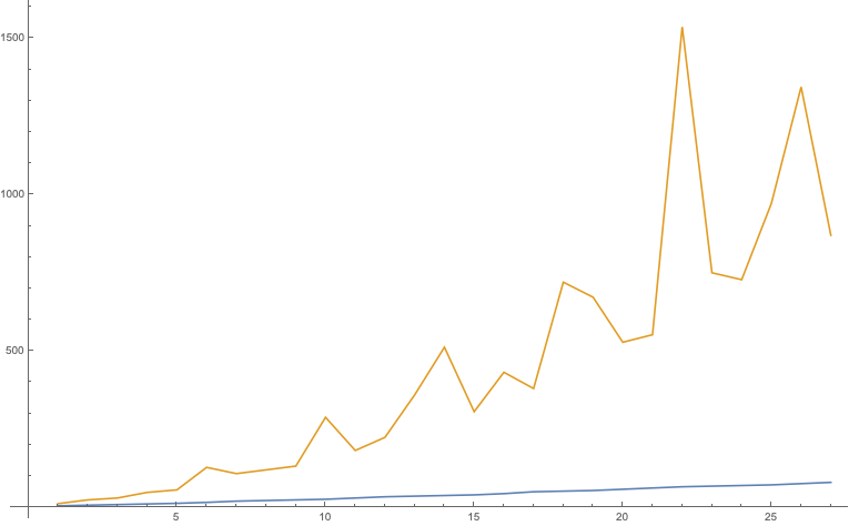
We notice that there are peaks for composite values of $N.$ Therefore we have many more points inside the box, for AdS${}_{2}[N],$ than on AdS${}_{2}[\mathbb{Z}].$ The additional points count the equivalence classes of points of AdS${}_{2}[\mathbb{Z}]$ mod $N.$

From these results we deduce that, for large $N,$ the number of solutions, mod$\,N,$ scales like the area, i.e. $N^{2}.$ So most of the points of AdS${}_{2}[N]$ are close to its boundary and holography is possible in this case too [59].

4 Continuum limit for large $N$

4.1 All solutions of $M^{2}\equiv\,1\,\mathrm{mod}\,N$

In section 2.3, we constructed the discrete geometry AdS${}_{2}[N]$ by introducing, first, a UV cutoff ($a=R_{\mathrm{AdS_{2}}}/M,$ with $M$ integer) and, also, an IR cutoff $L=Na,$ with $N$ another integer, bigger than $M.$

The continuum limit is defined by any sequence of pairs of integers, $(M_{n},N_{n}),$ $n=1,2,3,\ldots,$ such that, for any $n,$ (a) $N_{n}>M_{n},$ (b) $M_{n}^{2}\equiv\,1\,\mathrm{mod}\,N_{n},$ and (c) the limit of the ratio $N_{n}/M_{n}$ takes a finite value, $>1$ (as $n\to\infty$), which we can identify with $L/R_{\mathrm{AdS}_{2}}.$

Below we shall present the general solution to the equation $M^{2}\equiv\,1\,\mathrm{mod}\,N.$ Subsequently, we shall pick those solutions that satisfy the other requirements.

The first step is to factor $N$ into (powers of) primes, $N=q_{1}^{k_{1}}q_{2}^{k_{2}}\cdots q_{l}^{k_{l}}.$ Then the equation $M^{2}\equiv\,1\,\mathrm{mod}\,N,$ is equivalent to the system

$$M_{I}^{2}\equiv\,1\,\mathrm{mod}\,q_{I}^{k_{I}}$$ (4.1)

where $I=1,2,\ldots,l.$ The Chinese Remainder Theorem [52] then implies that all the solutions of eq. (4.1) can be used to construct $M,$ with $M=M_{1}m_{1}n_{1}+\cdots M_{l}m_{l}n_{l},$ where $M_{I}\equiv\,M\,\mathrm{mod}\,q_{I}^{k_{I}},$ $m_{I}=M/M_{I},$ $n_{I}\,\equiv m_{I}^{-1}\,\mathrm{mod}\,M_{I}.$

When $q_{I}\neq 2,$ the solutions are $M_{I}=1$ and $q_{I}^{n_{I}}-1.$ When $q_{I}=2,$ there exist four solutions, $M_{I}=1,2^{n_{I}}-1,2^{n_{I}-1}\pm 1.$

Now we must choose sequences, $N_{n}$ and determine the corresponding $M_{n},$ satisfying the constraints listed above.

In the next subsection(s) we shall present interesting sequences of pairs, $(M_{n},N_{n})$ of such solutions, whose limiting ratio, $\lim_{n\to\infty}N_{n}/M_{n},$ is the “golden” or “silver” ratios.

4.2 Fibonacci sequences for the UV/IR cutoffs

Although it is easy to demonstrate the existence of such sequences–for example, $N_{n}=2^{n}$ and $M_{n}=2^{n-1}\pm 1,$ where $M_{n}^{2}\equiv\,1\,\mathrm{mod}\,N_{n}$ and $N_{n}/M_{n}\to 2,$ in this section we focus on a particular class of sequences, based on the Fibonacci numbers, $f_{n}$ [52]. This case is of particular interest, since, in our previous paper [32], where we studied fast scrambling, we found that, for geodesic observers, moving in AdS${}_{2}[N],$ with evolution operator the Arnol’d cat map, the fast scrambling bound is saturated, when $N$ is a Fibonacci integer.

The Fibonacci sequence, defined by

$$\begin{array}[]{l}f_{0}=0;f_{1}=1\\ f_{n+1}=f_{n}+f_{n-1}\\ \end{array}$$ (4.2)

can be written in matrix form

$$\left(\begin{array}[]{c}f_{n}\\ f_{n+1}\end{array}\right)=\underbrace{\left(\begin{array}[]{cc}0&1\\ 1&1\end{array}\right)}_{\sf A}\left(\begin{array}[]{c}f_{n-1}\\ f_{n}\end{array}\right)$$ (4.3)

We remark that the famous Arnol’d cat map can be written as

$$\left(\begin{array}[]{cc}1&1\\ 1&2\end{array}\right)={\sf A}^{2}$$ (4.4)

Since the matrix ${\sf A}$ doesn’t depend on $n,$ we can solve the recursion relation in closed form, by setting $f_{n}\equiv C\rho^{n}$ and find the equation, satisfied by $\rho$

$$\rho^{n+1}=\rho^{n}+\rho^{n-1}\Leftrightarrow\rho^{2}-\rho-1=0\Leftrightarrow\rho\equiv\rho_{\pm}=\frac{1\pm\sqrt{5}}{2}$$

Therefore, we may express $f_{n}$ as a linear combination of $\rho_{+}^{n}$ and $\rho_{-}^{n}=(-)^{n}\rho_{+}^{-n}$:

$$f_{n}=A_{+}\rho_{+}^{n}+A_{-}\rho_{-}^{n}\Leftrightarrow\left\{\begin{array}[]{l}f_{0}=A_{+}+A_{-}=0\\ f_{1}=A_{+}\rho_{+}+A_{-}\rho_{-}=1\end{array}\right.$$ (4.5)

whence we find that

$$A_{+}=-A_{-}=\frac{1}{\rho_{+}-\rho_{-}}=\frac{1}{\sqrt{5}}$$

therefore,

$$f_{n}=\frac{\rho_{+}^{n}-(-)^{n}\rho_{+}^{-n}}{\sqrt{5}}$$ (4.6)

It’s quite fascinating that the LHS of this expression is an integer!

The eigenvalue $\rho_{+}>1$ is known as the “golden ratio” (often denoted by $\phi$) and it’s straightforward to show that $f_{n+1}/f_{n}\to\rho_{+},$ as $n\to\infty.$

Furthermore, it can be shown, by induction, that the elements of ${\sf A}^{n}$ are, in fact, the Fibonacci numbers themselves, arranged as follows:

$${\sf A}^{n}=\left(\begin{array}[]{cc}f_{n-1}&f_{n}\\ f_{n}&f_{n+1}\end{array}\right)$$ (4.7)

One reason this expression is useful is that it implies that $\mathrm{det}\,{\sf A}^{n}=(-)^{n}=f_{n-1}f_{n+1}-f_{n}^{2}.$

For $n=2l+1,$ we remark that this relation takes the form $f_{2l+1}^{2}=1+f_{2l}f_{2l+2}.$

Now, since $f_{2l+1}$ and $f_{2l+2}$ are successive iterates, they’re coprime, which implies, that $f_{2l+1}^{2}\equiv\,1\,\mathrm{mod}\,f_{2l+2}.$

Therefore, the sequence of pairs, $(M_{l}=f_{2l+1},N_{l}=f_{2l+2}),$ where $l=1,2,3,\ldots,$ satisfy all of the requirements and the corresponding limiting ratio, $L/R_{\mathrm{AdS_{2}}},$ can be found analytically. It is, indeed, equal to $\rho_{+}=(1+\sqrt{5})/2,$ the golden ratio.

We recall here that the periods of the Fibonacci sequence mod $N,$ for any integer $N,$ has been analyzed in the literature (cf. [60]) and, in the case when $N,$ the IR cutoff, is, itself, a Fibonacci integer, then the period of the corresponding Arnol’d cat map grows logarithmically with $N$ and this is the reason for the saturation of the fast scrambling bound [32]. In the next subsection we shall consider the so-called $k-$Fibonacci sequences, which will be important for removing the IR cutoff.

4.3 Generalized Fibonacci sequences and UV/IR cutoffs

It’s possible to generalize the Fibonacci sequence in the following way:

$$g_{n+1}=kg_{n}+g_{n-1}$$ (4.8)

with $g_{0}=0$ and $g_{1}=1$ and $k$ an integer. This is known as the “$k-$Fibonacci” sequence [61].

We may solve for $g_{n}\equiv C\rho^{n}$; the characteristic equation for $\rho,$ now, reads

$$\rho^{2}-k\rho-1=0\Leftrightarrow\rho_{\pm}(k)=\frac{k\pm\sqrt{k^{2}+4}}{2}$$ (4.9)

and express $g_{n}$ as a linear combination of the $\rho_{\pm}$:

$$g_{n}=A_{+}\rho_{+}(k)^{n}+A_{-}\rho_{-}(k)^{n}=\frac{\rho_{+}(k)^{n}-(-)^{n}\rho_{+}(k)^{-n}}{\sqrt{k^{2}+4}}$$ (4.10)

that generalizes eq. (4.6).

In matrix form

$$\left(\begin{array}[]{c}g_{n}\\ g_{n+1}\end{array}\right)=\underbrace{\left(\begin{array}[]{cc}0&1\\ 1&k\end{array}\right)}_{{\sf A}(k)}\left(\begin{array}[]{c}g_{n}\\ g_{n-1}\end{array}\right)$$ (4.11)

Similarly as for the usual Fibonacci sequence, we may show, by induction, that

$${\sf A}(k)^{n}=\left(\begin{array}[]{cc}g_{n-1}&g_{n}\\ g_{n}&g_{n+1}\end{array}\right)$$ (4.12)

We find that $\mathrm{det}\,{\sf A}(k)^{n}=(-)^{n},$ therefore that $g_{2l+1}^{2}\equiv\,1\,\mathrm{mod}\,g_{2l+2}$; thus, $g_{2l+2}/g_{2l+1}\to L/R_{\mathrm{AdS_{2}}}=\rho_{+}(k),$ where the eigenvalue of ${\sf A}(k),$ $\rho_{+}(k),$ that’s greater than 1, of course, depends on $k.$ At this point we have determined $L,$ the IR cutoff, in terms of $R_{\mathrm{AdS_{2}}}.$ This limiting procedure has removed the UV cutoff, since $a\to 0,$ however the IR cutoff, $L$ is, still, present.

What is remarkable is that, using the additional parameter, $k,$ of the $k-$Fibonacci sequence, it is possible to remove the IR cutoff, as well, since it is possible to send $L\to\infty,$ as $k\to\infty,$ keeping $R_{\mathrm{AdS_{2}}}$ fixed.

If $k$ remains finite, the periodic box cannot be removed and, in the continuum limit, $a\to 0,$ we obtain infinitely many foldings of the AdS₂ surface inside the box due to the mod $L$ operation.

The Fibonacci sequence, taken mod $N,$ is periodic, with period $T(N)$; this turns out to be a “random” function of $N.$ The “shortest” periods, as has been shown by Falk and Dyson [60], occur when $N=F_{l},$ for any $l.$ In that case, $T(F_{l})=2l.$

We may, thus, ask the same question for the $k-$Fibonacci sequence, where the ratio of its successive elements, $g_{n+1}/g_{n}$ tend to the so-called “$k-$silver ratio”,

$$\rho_{+}(k)=\frac{k+\sqrt{k^{2}+4}}{2}$$ (4.13)

(the “silver ratio” is $\rho_{+}(k=2)$)

From eq. (4.12), taking mod $g_{l}$ on both sides, we find that, when $n=l,$ the matrix becomes $\pm$(the identity matrix), so $T(g_{l})=l$ or $2l,$ respectively; thereby generalizing the Falk–Dyson result for the $k-$Fibonacci sequences. Since, for large $l,$ $g_{l}\sim e^{l\log\rho_{+}(k)},$ $\log\rho_{+}(k)$ can be identified with the Lyapunov exponent of the dynamics of the ${\sf A}(k)$ map. What is interesting in this generalization is that $\rho_{+}(k)\sim k,$ so, for, large $k,$ can become significantly larger than the Lyapunov exponent of the Arnol’d cat map–so the scrambling time is significantly shorter.

5 Discussion and open issues

In this work we have proposed a construction of the continuum AdS₂ radial and time near horizon geometry of extremal black holes from a finite and arithmetic geometry, AdS${}_{2}[N],$ for every integer $N.$ This entails the introduction of UV and IR cutoffs, respectively $a=R_{\mathrm{AdS_{2}}}/M$ and $L=aN,$ where $L>R_{\mathrm{AdS_{2}}}$ is the size of the periodic box, that encloses the one–sheeted hyperboloid.

The periodic box and the UV cutoff deform the SL$(2,\mathbb{R})$ isometry of AdS₂ to the finite group, $SL_{2}(\mathbb{Z}_{N}),$ which is the mod $N$ reduction of SL${}_{2}[\mathbb{Z}].$

The elements of this finite group are discrete maps and describe the evolution operators of the avatars of infalling observers, with proper time the iteration time of the corresponding maps.

For particular maps, such as the Arnol’d cat map and its $k-$Fibonacci generalizations, we find that they are chaotic, mixing and their mixing time time saturates the scrambling time bound [21, 22].

It seems today that theoretical high energy physics is passing through a paradigm shift from the elementary harmonic oscillator and relativistic quantum mechanics to the qubit of information and the measurement of complexity for discrete or continuous quantum systems. This was necessary in order to understand the gravitational force as an information measure of complex quantum systems. The prominent example is the AdS/CFT correspondence and the relation of quantum entanglemnt of the boundary conformal field theories with purely geometric objects of classical theories of gravitation. This holographic duality is indeed in analogy with the redundacy and the associated compression of information necessary for fast processing in complex systems.

The notion of locality in gravity is expressed in terms of the diffeomorphism invariance of the gravitational action. This implies the absence of local observables and only in the case of well defined asymptotic behavior of the metric, conformal or not, do there exist globally defined observables, that can characterize the gravitational background. In the case of the AdS/CFT correspondence, the holographic dualities are restricted by the UV/IR correspondence and locality is lost both in the boundary as well as in the bulk.

On the other hand,, the present efforts to understand the near horizon region, as well as the interior and the exterior of black holes, which are asymptotically anti-de Sitter, rely exclusively on the boundary CFT point of view. This approach, however, reaches its limit when attempting to resolve features, beyond the Planck scale, where no formalism for performing reliable calculations is, to date, available.

For these reasons our program for using the arithmetic of finite geometries has an intrinsic interest as an alternative way for reconstructing bulk spacetimes, as emerging in an appropriate scaling limit thereof. Among the main advantages are:

• As shown in this paper this scaling limit is the correct one, in that the usual, continuum, AdS₂ geometry is recovered–this is a very important sanity check.

• The relation of finite geometries to quantum information theory and their representation as quantum circuits with measurable complexity [62, 63, 64, 65]. It, also, provides a framework for quantitatively studying the Eigenstate Thermalization Hypothesis [66] and the fast scrambling bound [32].

• Due to the modular arithmetic, an intrinsic number theoretic randomness appears in the geometry itself, as well as in the dynamics of wave packets with finite dimensional Hilbert space [58].

In the present work we established the modular geometry AdS${}_{2}[N]$ as a useful toy model that realizes many of the basic properties, for the near horizon geometries of extremal/near extremal black holes, such as holography, non–locality of the geometry and the fast mixing dynamics of particle probes, that saturate the scrambling time bound.

Along the way, we discussed interesting methods to localize and count the integral points of the AdS₂ continuous geometry and to characterize the points of AdS${}_{2}[N]$ as equivalence classes of the AdS₂ integral points modulo the congruent modular group $\Gamma[N].$ The continuouus limit of the modular geometry AdS${}_{2}[N]$ was constructed explicitly, using infinite sequences of UV/IR cutoffs $(M_{n},N_{n}),n=1,2,\ldots,$ taken from the integer sequences of the $k-$Fibonacci numbers.

The sequence of UV cutoffs,$N_{n}$ describes the dimension of the Hilbert space of states of single–particle probes and, in the case of $k-$Fibonacci sequence, $k=1,2,\ldots,$ the dynamics of the corresponding cat maps saturates the scarmbling time bound with a Lyapunov exponent that grows logarithmically with $k.$

Among the open issues of our approach we may mention:

• The extension to modular discretizations of higher dimensional AdS/CFT duals, using the corresponding arithmetic isometry groups.

• The extension to the BTZ black hole.

• Describing de Siter spacetimes [67] using arithmetic geometry.

• Many–body probe systems and the ensuing questions related to their entanglement and the time behaviour of their OTOC bulk quantum correlators.

These issues are technically feasible and physically interesting with available tools.

We should stress that we are still far from proposing a complete framework suitable to study the fluctutations, due to quantum gravity itself, on such discrete backgrounds.It will be necessary to express the metric in information-theoretic terms,or more directly in the case of AdS${}_{2}[N]$ through the relation of geodesic distance and the quantum mechanical coherent states [34], as well as to formulate a discrete (gravitational) action principle at Planckian scales.In our discrete time setting we should rather construct a unitary evolution operator in the space of metrics.Another possible direction t o this end could the relation of the modular with the $p-$adic AdS₂ geometry, [68, 69] and referencs therein.

Acknowledegements: This work spanned many places and benefitted from discussions with many people. We would like to thank, in particular, Costas Bachas and John Iliopoulos at the LPTENS, Alex Kehagias, Boris Pioline, Kyriakos Papadodimas and Eliezer Rabinovici at CERN. We acknowledge the warm hospitality at Ecole Normale Supérieure, Paris, the Theory Division at CERN and the Institute of Nuclear and Particle Physics of the NRCPS “Demokritos”.

References

- [1] G. ’t Hooft, “How quantization of gravity leads to a discrete space-time,” J. Phys. Conf. Ser. 701 no. 1, (2016) 012014.
- [2] E. Witten, “Superstring Perturbation Theory Revisited,” arXiv:1209.5461 [hep-th].
- [3] E. Witten, “More On Superstring Perturbation Theory: An Overview Of Superstring Perturbation Theory Via Super Riemann Surfaces,” arXiv:1304.2832 [hep-th].
- [4] E. Witten, “String theory dynamics in various dimensions,” Nucl. Phys. B443 (1995) 85–126, arXiv:hep-th/9503124 [hep-th]. [,333(1995)].
- [5] T. Banks, W. Fischler, S. H. Shenker, and L. Susskind, “M theory as a matrix model: A Conjecture,” Phys. Rev. D55 (1997) 5112–5128, arXiv:hep-th/9610043 [hep-th]. [,435(1996)].
- [6] W. Taylor, “M(atrix) theory: Matrix quantum mechanics as a fundamental theory,” Rev. Mod. Phys. 73 (2001) 419–462, arXiv:hep-th/0101126 [hep-th].
- [7] A. Almheiri, X. Dong, and D. Harlow, “Bulk Locality and Quantum Error Correction in AdS/CFT,” JHEP 04 (2015) 163, arXiv:1411.7041 [hep-th].
- [8] G. Veneziano, “A Model for the big bounce,” JCAP 0403 (2004) 004, arXiv:hep-th/0312182 [hep-th].
- [9] L. Cornalba, M. S. Costa, and C. Kounnas, “A resolution of the cosmological singularity in string theory,” Astrophys. Space Sci. 283 (2003) 517–524.
- [10] D. Christodoulou, “Reversible and irreversible transforations in black hole physics,” Phys. Rev. Lett. 25 (1970) 1596–1597.
- [11] J. M. Bardeen, B. Carter, and S. W. Hawking, “The four laws of black hole mechanics,” Communications in Mathematical Physics 31 no. 2, (Jun, 1973) 161–170. https://doi.org/10.1007/BF01645742.
- [12] J. D. Bekenstein, “Black holes and entropy,” Phys. Rev. D7 (1973) 2333–2346.
- [13] S. W. Hawking, “Particle Creation by Black Holes,” Commun. Math. Phys. 43 (1975) 199–220. [,167(1975)].
- [14] S. W. Hawking, “Black Holes and Thermodynamics,” Phys. Rev. D13 (1976) 191–197.
- [15] G. ’t Hooft, “The black hole interpretation of string theory,” Nucl. Phys. B335 (1990) 138–154.
- [16] G. ’t Hooft, “Dimensional reduction in quantum gravity,” Conf. Proc. C930308 (1993) 284–296, arXiv:gr-qc/9310026 [gr-qc].
- [17] L. Susskind, L. Thorlacius, and J. Uglum, “The Stretched horizon and black hole complementarity,” Phys. Rev. D48 (1993) 3743–3761, arXiv:hep-th/9306069 [hep-th].
- [18] L. Susskind, “The World as a hologram,” J. Math. Phys. 36 (1995) 6377–6396, arXiv:hep-th/9409089 [hep-th].
- [19] J. A. Wheeler, “Feynman and computation,” ch. Information, Physics, Quantum: The Search for Links, pp. 309–336. Perseus Books, Cambridge, MA, USA, 1999. http://dl.acm.org/citation.cfm?id=304763.305702.
- [20] R. Bousso, “The Holographic principle,” Rev. Mod. Phys. 74 (2002) 825–874, arXiv:hep-th/0203101 [hep-th].
- [21] P. Hayden and J. Preskill, “Black holes as mirrors: Quantum information in random subsystems,” JHEP 09 (2007) 120, arXiv:0708.4025 [hep-th].
- [22] Y. Sekino and L. Susskind, “Fast Scramblers,” JHEP 10 (2008) 065, arXiv:0808.2096 [hep-th].
- [23] L. Susskind, “Addendum to Fast Scramblers,” arXiv:1101.6048 [hep-th].
- [24] S. W. Hawking, “Black holes and unpredictability.,” Physics Bulletin 29 (Jan, 1978) 23.
- [25] S. W. Hawking, “Information loss in black holes,” Phys. Rev. D72 (2005) 084013, arXiv:hep-th/0507171 [hep-th].
- [26] J. M. Maldacena, “The Large N limit of superconformal field theories and supergravity,” Int. J. Theor. Phys. 38 (1999) 1113–1133, arXiv:hep-th/9711200 [hep-th]. [Adv. Theor. Math. Phys.2,231(1998)].
- [27] E. Witten, “Anti-de Sitter space and holography,” Adv. Theor. Math. Phys. 2 (1998) 253–291, arXiv:hep-th/9802150 [hep-th].
- [28] E. Witten, “Anti-de Sitter space, thermal phase transition, and confinement in gauge theories,” Adv. Theor. Math. Phys. 2 (1998) 505–532, arXiv:hep-th/9803131 [hep-th]. [,89(1998)].
- [29] S. Banerjee, J.-W. Bryan, K. Papadodimas, and S. Raju, “A toy model of black hole complementarity,” JHEP 05 (2016) 004, arXiv:1603.02812 [hep-th].
- [30] R. Penrose, The Road to Reality: A Complete Guide to the Laws of the Universe. Vintage Books, 2007.
- [31] E. Frenkel, “Lectures on the Langlands program and conformal field theory,” in Proceedings, Les Houches School of Physics: Frontiers in Number Theory, Physics and Geometry II: On Conformal Field Theories, Discrete Groups and Renormalization: Les Houches, France, March 9-21, 2003, pp. 387–533. 2007. arXiv:hep-th/0512172 [hep-th].
- [32] M. Axenides, E. Floratos, and S. Nicolis, “The quantum cat map on the modular discretization of extremal black hole horizons,” Eur. Phys. J. C78 no. 5, (2018) 412, arXiv:1608.07845 [hep-th].
- [33] M. Axenides, E. Floratos, and S. Nicolis, “Chaotic Information Processing by Extremal Black Holes,” Int. J. Mod. Phys. D24 no. 09, (2015) 1542012, arXiv:1504.00483 [hep-th].
- [34] M. Axenides, E. G. Floratos, and S. Nicolis, “Modular discretization of the AdS2/CFT1 holography,” JHEP 02 (2014) 109, arXiv:1306.5670 [hep-th].
- [35] P. Claus, M. Derix, R. Kallosh, J. Kumar, P. K. Townsend, and A. Van Proeyen, “Black holes and superconformal mechanics,” Phys. Rev. Lett. 81 (1998) 4553–4556, arXiv:hep-th/9804177 [hep-th].
- [36] J. L. F. Barbón and J. M. Magán, “Fast Scramblers And Ultrametric Black Hole Horizons,” JHEP 11 (2013) 163, arXiv:1306.3873 [hep-th].
- [37] S. Pramodh and V. Sahakian, “From Black Hole to Qubits: Evidence of Fast Scrambling in BMN theory,” JHEP 07 (2015) 067, arXiv:1412.2396 [hep-th].
- [38] N. Lashkari, D. Stanford, M. Hastings, T. Osborne, and P. Hayden, “Towards the Fast Scrambling Conjecture,” JHEP 04 (2013) 022, arXiv:1111.6580 [hep-th].
- [39] J. L. F. Barbon and J. M. Magan, “Fast Scramblers Of Small Size,” JHEP 10 (2011) 035, arXiv:1106.4786 [hep-th].
- [40] A. Schild, “Discrete Space-Time and Integral Lorentz Transformations,” Canadian J. Math. 1 (1949) 29–47.
- [41] A. Schild, “Discrete Space-Time and Integral Lorentz Transformations,” Phys. Rev. 73 (Feb, 1948) 414–415. https://link.aps.org/doi/10.1103/PhysRev.73.414.
- [42] V. G. Kac, Infinite dimensional Lie algebras. Cambridge, UK: Univ. Pr. (1990) 400 p, 1990. http://www.cambridge.org/uk/catalogue/catalogue.asp?isbn=0521372151.
- [43] W. Duke, Z. Rudnick, and P. Sarnak, “Density of integer points on affine homogeneous varieties,” Duke Math. J. 71 no. 1, (07, 1993) 143–179. https://doi.org/10.1215/S0012-7094-93-07107-4.
- [44] I. Bengtsson, Anti-de Sitter space. http://http://3dhouse.se/ingemar/Kurs.pdf.
- [45] G. W. Gibbons, “Anti-de-Sitter spacetime and its uses,” in Mathematical and quantum aspects of relativity and cosmology. Proceedings, 2nd Samos Meeting on cosmology, geometry and relativity, Pythagoreon, Samos, Greece, August 31-September 4, 1998, pp. 102–142. 2011. arXiv:1110.1206 [hep-th]. http://springerlink.metapress.com/openurl.asp?genre=article&issn=1616-6361&volume=537&spage=102.
- [46] M. Cadoni and S. Mignemi, “Asymptotic symmetries of AdS(2) and conformal group in d = 1,” Nucl. Phys. B557 (1999) 165–180, arXiv:hep-th/9902040 [hep-th].
- [47] C. Patricot, “A Group theoretical approach to causal structures and positive energy on space-times,” arXiv:hep-th/0403040 [hep-th].
- [48] J. Rawnsley, “On the universal covering group of the real symplectic group,” Journal of Geometry and Physics 62 no. 10, (2012) 2044 – 2058. http://www.sciencedirect.com/science/article/pii/S039304401200112X.
- [49] D. Shanks, “A sieve method for factoring numbers of the form ,” Mathematical Tables and Other Aids to Computation 13 no. 66, (1959) 78–86. http://www.jstor.org/stable/2001956.
- [50] A. Baragar, “Lattice points on hyperboloids of one sheet,” New York Journal of Mathematics 20 (2014) 1253–1268. http://nyjm.albany.edu/j/2014/20-58.html.
- [51] A. V. Kontorovich, “The Hyperbolic Lattice Point Count in Infinite Volume with Applications to Sieves,” arXiv e-prints (Dec, 2007) arXiv:0712.1391, arXiv:0712.1391 [math.NT].
- [52] D. Bressoud and S. Wagon, A Course in Computational Number Theory. No. vol. 1 in A Course in Computational Number Theory. Key College Pub., 2000. https://books.google.gr/books?id=JEc_AQAAIAAJ.
- [53] L. Tan, “Rational points on the circle,” Mathematics Magazine 69 no. 3, (1996) 163–171.
- [54] H. S. M. Coxeter, “Discrete groups generated by reflections,” Annals of Mathematics 35 no. 3, (1934) 588–621. http://www.jstor.org/stable/1968753.
- [55] È. B. Vinberg, “Discrete Groups generated by reflections in Lobačevskiĭ spaces,” Mathematics of the USSR-Sbornik 1 no. 3, (Apr, 1967) 429–444. https://doi.org/10.1070%2Fsm1967v001n03abeh001992.
- [56] A. J. Feingold, A. Kleinschmidt, and H. Nicolai, “Hyperbolic Weyl groups and the four normed division algebras,” J. Algebra 322 (2009) 1295–1339, arXiv:0805.3018 [math.RT].
- [57] V. I. Arnol’d and A. Avez, Ergodic problems of classical mechanics. The mathematical physics monograph series. W. A. Benjamin, New York, NY, 1968. http://cds.cern.ch/record/1987366.
- [58] G. G. Athanasiu and E. G. Floratos, “Coherent states in finite quantum mechanics,” Nucl. Phys. B425 (1994) 343–364.
- [59] L. Susskind and E. Witten, “The holographic bound in Anti-de Sitter space,” arXiv:hep-th/9805114 [hep-th].
- [60] F. J. Dyson and H. Falk, “Period of a discrete cat mapping,” The American Mathematical Monthly 99 no. 7, (1992) 603–614. http://www.jstor.org/stable/2324989.
- [61] A. F. Horadam, “A Generalized Fibonacci Sequence,” The American Mathematical Monthly 68 no. 5, (1961) 455–459. http://www.jstor.org/stable/2311099.
- [62] L. Susskind, “Black Holes and Complexity Classes,” arXiv:1802.02175 [hep-th].
- [63] L. Susskind, “Three Lectures on Complexity and Black Holes,” 2018. arXiv:1810.11563 [hep-th].
- [64] R. Jefferson and R. C. Myers, “Circuit complexity in quantum field theory,” JHEP 10 (2017) 107, arXiv:1707.08570 [hep-th].
- [65] J. Preskill, “Quantum information and physics: some future directions,” J. Mod. Opt. 47 (2000) 127–137, arXiv:quant-ph/9904022 [quant-ph].
- [66] M. Srednicki, “Chaos and quantum thermalization,” Phys. Rev. E 50 (Aug, 1994) 888–901. https://link.aps.org/doi/10.1103/PhysRevE.50.888.
- [67] E. Witten, “Quantum gravity in de Sitter space,” in Strings 2001: International Conference Mumbai, India, January 5-10, 2001. 2001. arXiv:hep-th/0106109 [hep-th].
- [68] C.-T. Ma, “Lattice AdS Geometry and Continuum Limit,” arXiv:1807.08871 [hep-th].
- [69] S. S. Gubser, “A -adic version of AdS/CFT,” Adv. Theor. Math. Phys. 21 (2017) 1655–1678, arXiv:1705.00373 [hep-th].