How many ways to color the map of America?

Abstract

Although the Four Color Conjecture originated in cartography, surprisingly, there is nothing in the literature on the number of ways to color an actual geographic map with four or less colors. In this paper, we compute these numbers, with exponentially increasing order of difficulty, for the maps of Canada, France, and the USA. Our attempts to compute the latter two lead to some new results on the chromatic polynomial of graphs.

1 Introduction

The Four Color Theorem conjectured by Francis Guthrie in 1852, asserts that no planar graph needs more than four colors to color it properly. A coloring is proper if no two vertices which are adjacent are assigned the same color. A related problem, on which we found no literature for real life graphs, is to determine the number of ways to color the graph $G_{X}$ of a given country X, with $k(G_{X})\leq 4$ colors, $k(G_{X})$ being the smallest number of colors with which $G_{X}$ can be colored properly. It is easy to see that $k(G_{X})=3$ if $G_{X}$ is the graph of the map of the provinces/territories of Canada. However, a Google search found no entry for the number of ways to color the map of Canada with three colors. As we will show this number is 576 and fairly easy to compute by hand. But this is not so easy for the map of the contiguous regions of France. There are programs which use the computing power of a machine that will find this number for the main part of France which has twelve contiguous regions. In fact, we used different programs to compute and compare this number for the map of the 29 counties of the state Utah of USA. However, these programs reach their limit when the number of the vertices of a graph is around 40. Although the Four Color Conjecture originated in Cartography, surprisingly, there is no revert to cartography.

Some years ago, a Google search found only one site that gave without any justification or reference, the number of ways to color the map of USA. This number was claimed to be somewhere between 20 and 21 trillion, but soon taken off the web. This left us wondering what exactly this number is. The purpose of this paper is to compute, just out of curiosity, this number for the metropolitan regions of France and the lower 48 states of the USA and prove some theorems the authors discovered on chromatic polynomials in their attempts to compute this number, for France and for the USA.

2 Preliminaries

A graph is a pair $(V,G)$ with a non-empty set $V=V(G)$ of its vertices and a subset $E=E(G)\subset P_{2}(V)$ of its edges, $E$ possibly empty. Here $P_{2}(V)$ is the set of all sets $T\subset V$ with the carnality $|T|=2$. To fix the notation, the following examples of graphs will appear throughout this paper. It is convenient to represent the elements of V by dots and also call them points, whereas an edge $\{u,v\}$ in $E(G)$ will be represented by . We call u,v adjacent or neighbors. All the Graphs $G$ considered in this paper are finite, i.e. $|V(G)|<\infty$.

1. Path. $P_{n}$ of length $n-1(n\geq 2)$. We call $v_{1}$ and $v_{n}$ its endpoints.

2. Cycle. $C_{n}$ on $n$ vertices $(n\geq 3)$ is obtained from $P_{n+1}$ by identifying its end points.

Figure 1: Cycles

3. Complete graph. $G=K_{n}$ Here $|V(G)|=n$ and $E(G)=P_{2}(V)$, i.e. every two vertices $u,v$ of $G$ are adjacent.

4. Wheel. $W_{n}$ on $n$ vertices $(n\geq 4)$.

Figure 2: Wheels

Two graphs $G_{1}=(V_{1},E_{1})$ and $G_{2}=(V_{2},E_{2})$ are isomorphic, written as $G_{1}\cong G_{2}$, if there is a bijection $f:V_{1}\longrightarrow V_{2}$ such that $\{u,v\}\in E_{1}\Longleftrightarrow\{f(u),f(v)\}\in E_{2}$. For example, $P_{2}\cong K_{2}$ and $K_{4}\cong W_{4}$.

5. Real Life Graphs. By these we mean the graphs associated to, among others, the geographic entities such as the map of the USA. In this graph, the vertices are the states of the USA and two states are adjacent if they share a non-trivial border, a border of positive length. Thus, for our purpose, the states of Arizona and Colorado are not adjacent, and can be given the same color.

A graph $G$ is connected if for any two vertices $u,v$ in $V(G)$, there is a path in $G$ with $u,v$ as its end points. A subgraph of $G=(V,E)$ is a graph $(V^{\prime},E^{\prime})$ with $V^{\prime}\subseteq V$ and $E^{\prime}\subseteq P_{2}(V^{\prime})\cap E$. A largest connected subgraph of a graph is its connected component. For example, the graph of the USA has 3 connected components. We will be concerned only with its largest connected components $G_{A}$, comprising of its lower 48 states.

3 Coloring Problem

A coloring of a graph $G$ with $t$ colors is simply a map $f:V(G)\longrightarrow C$, where $C$ is a set of given $t$ colors. The coloring is proper if $f(u)\neq f(v)$ whenever $\{u,v\}\in E(G)$, i.e. no two adjacent vertices are given the same color. Throughout this paper, by coloring we mean only proper coloring.

The chromatic number of a graph is the cardinality $k(G)=|C|$ of a smallest set $C$ of colors such that there is at least one way $f:V(G)\longrightarrow C$ to color it with $k(G)$ colors in $C$. The following examples will be used throughout our presentation.

1. $k(P_{n})=2$.

2. $k(C_{n})=\begin{cases}2&\text{if {n} is even}\\ 3&\text{if {n} is odd.}\end{cases}$


3. $k(W_{6})=4.$

4. If $G_{C}$ is the graph of the map of Canada, it is easy to check that $k(G_{C})=3$.

5. Since the graph $G_{A}$ of the lower 48 states of America contains a $W_{6}$ centered at Nevada (cf. Figure 16) as a subgraph, $k(G_{A})\geq 4$. By the Four Color Theorem, $k(G_{A})=4$.

A graph is planar if it can be drawn on a plane or equivalently on a sphere, without any edges crossing. All geographic maps with contiguous parts (states, provinces, districts, etc.) are planar. The Petersen graph is an example of a non-planar graph, but it does not concern us as all graphs considered here are planar.

We denote the number of ways to color a graph $G$ by a set $C$ of $t$ colors by $\chi(G,t)$. Clearly it is the cardinality of the set {$f:V(G)\longrightarrow C|\text{ {f} is a proper coloring}$ }. It turns out that the function $\chi(G,t)$ has the following properties(cf. [1], [2]).

1. It is given by a polynomial in $t$ over $\mathbb{Z}$ (called the chromatic polynomial of $G$).

2. The degree $n$ of $\chi(G,t)$ is $|V(G)|$.

3. $\chi(G,t)$ is monic, i.e. its leading coefficient is 1.

4. The coefficient of $t^{n-1}$ is $-|E(G)|$.

5. The constant term of $\chi(G,t)$ is zero.

6. The coefficients of $\chi(G,t)$ are alternately positive and negative.

7. The degree of the lowest term in $\chi(G,t)$ is the number of components of $G$.

8. If $|V(G)|\geq 2$, the sum of all the coefficients of $\chi(G,t)$ is zero.

For convenience of the reader, we prove most of the properties of $\chi(G,t)$ and leave the rest as exercises.

Proofs.

Properties 5 and 8 are trivial. The constant term = $\chi(G,0)=0$, because there is no way to color $G$ with no colors. This proves 5. For 8, the sum of the coefficients of $\chi(G,t)$ is the same as $\chi(G,1)$, which is zero - since there is no way to color a connected graph $G$ with 1 color if $|V(G)|\geq 2$. ∎

The proof of property 1, 2, 3, and 6 we will be given in Section 5.

4 Chromatic Polynomials of Some Standard Graphs

The following is obvious.

Theorem 1. We have

1) $\chi(P_{n},t)=t(t-1)^{n-1}$,
2) $\chi(C_{3},t)=t(t-1)(t-2)$,
3) $\chi(K_{n},t)=t(t-1)(t-2)...(t-n+1)$.

The following requires proofs. A connected graph $T$ is a tree if it contains no cycle as a subgraph.

Theorem 2. If $T$ is a tree with $|V(T)|=n$, then $\chi(T,t)=t(t-1)^{n-1}$.

Theorem 3. If $n\geq 3$, then $\chi(C_{n},t)=(t-1)^{n}+(-1)^{n}(t-1)$.

Theorem 4. If $n\geq 4,$ then

$$\chi(W_{n},t)=t[(t-2)^{n-1}+(-1)^{n-1}(t-2)]$$ (1)

We will prove Theorems 3 and 4 for which, we will need the following two simple but powerful results, known as the Chromatic Reduction Theorems. In order to state and prove them, we recall some notation and terminology. If $e=\{u,v\}$ is an edge of a graph $G$, then $G-e$ is the graph $(V(G),E(G)-e)$, and $G\text{ mod }e$ is the graph $G/e$ obtained from $G-e$ by identifying $u$ and $v$. In the pictorial representation of $G/e$, we keep only one line between $u$ and $v$ if their identification creates extra lines between them.

Example 1. Let $e$ be the peripheral edge $\{2,3\}$ of the wheel $W_{6}$. Then the broken wheel $W^{\prime}_{6}=W_{6}-e$ and $W_{6}/e$ are illustrated in Figure 3.

Figure 3: The broken wheel $W^{\prime}_{6}$ and $W_{6}/e$

Now suppose that $G_{1}$ and $G_{2}$ are two graphs on disjoint sets of vertices and both $G_{1}$ and $G_{2}$ contain subgraphs that are isomorphic to a complete graph $K_{l}$. A graph $G$ is an overlap of $G_{1}$ and $G_{2}$ in $K_{l}$ if it is obtained by identifying the subgraphs of $G_{1}$ and $G_{2}$ that are isomorphic to $K_{l}$.

Example 2. Figure 4 illustrates two non-isomorphic overlaps of $G_{1}$ and $G_{2}$ in $K_{2}$.

Figure 4: Non-Isomorphic overlaps

Chromatic Reduction Theorem 1. (CRT-1) If $G$ is an overlap of $G_{1}$ and $G_{2}$ in $K_{l}$, then

$$\chi(G,t)=\frac{\chi(G_{1},t)\chi(G_{2},t)}{\chi(K_{l},t)}.$$ (2)

To prove it, just note that the denominator in the right hand side of (2) takes care of the repeated counting in the numerator due to the overlap in $K_{l}$.

Chromatic Reduction Theorem 2. (CRT-2) If $e=\{u,v\}$ is an edge of $G$, then

$\chi(G,t)=\chi(G-e,t)-\chi(G/e,t)$.

To prove it, note that $\chi(G-e,t)$ is the number of ways to color $G$ when u,v get the same color, which is $\chi(G/e,t)$, plus the number of ways to color $G$ when $v,u$ get different colors, which is $\chi(G,t)$.

Remarks.

1. It is easy to construct examples to show that CRT-1 is false if the overlap is not a complete graph.

2. Example 2 shows that two non-isomorphic graphs can have the same chromatic polynomial.

3. To compute the chromatic polynomial $\chi(G,t)$, there is no loss of generality to assume that $G$ is connected, because if $G_{1}$ and $G_{2}$ are its two connected components then $\chi(G,t)=\chi(G_{1},t)\chi(G_{2},t)$.

5 Application of Chromatic Reduction Theorems

As an easy application of the Chromatic Reduction Theorems, first we will prove Theorems 3 and 4. The proofs of Theorems 1 and 2 are easy and are left as an exercise for the reader.

Proof of Theorem 3.

We use induction on $n$. If $n=3$, the right hand side of the equation

$\chi(C_{n},t)=(t-1)^{n}+(-1)^{n}(t-1)$

is $(t-1)^{3}-(t-1)=(t-1)((t-1)^{2}-1)=t(t-1)(t-2)$ which is $\chi(C_{3},t)$. If $n\geq 3$, let $e$ be an edge of $C_{n+1}$. Then $C_{n+1}-e\cong P_{n+1}$ and $C_{n+1}/e\cong C_{n}$.
By CRT-2 and the Induction Hypothesis,

$$\chi(C_{n+1},t) =\chi(P_{n+1},t)-\chi(C_{n},t)$$

$$=t(t-n)^{n}-[(t-1)^{n}+(-1)^{n}(t-1)]$$

$$=(t-1)^{n+1}+(-1)^{n+1}(t-1)$$

This completes the proof by induction. ∎

In order to prove Theorem 4, we use the following terminology (See Figure 3). For $n\geq 5$, let $e$ be an edge on the rim of $W_{n}$. We call $W^{\prime}_{n}=W_{n}-e$ a broken wheel. Clearly, $W_{n}/e\cong W_{n-1}$. We also need the following.

Lemma. For $n\geq 4$, $\chi(W^{\prime}_{n+1},t)=t(t-1)(t-2)^{n-1}$.

Proof of Lemma.

Clearly, $W^{\prime}_{n+1}$ is an overlap of $C_{3}$ and $W^{\prime}_{n}$ in $K_{2}$. By CRT-1 and the Induction Hypothesis,

$$\chi(W^{\prime}_{n+1},t) =\frac{\chi(W^{\prime}_{n},t)\chi(C_{3},t)}{\chi(K_{2},t)}$$

$$=\frac{(t(t-1)(t-2)^{n-2})(t(t-1)(t-2))}{t(t-1)}$$

$$=t(t-1)(t-2)^{n-1}.$$

∎

Proof of Theorem 4.

It is again by induction on $n$. First let $n=4$. Since $W_{4}\cong K_{4}$, $\chi(W_{4},t)=\chi(K_{4},t)=t(t-1)(t-2)(t-3)$, which is the same as the right hand side of the equation (1) for $n=4$. Now let $n\geq 4$. Then by CRT-2 and the Induction Hypothesis,

$$\chi(W_{n+1},t) =\chi(W^{\prime}_{n+1},t)-\chi(W_{n},t)$$

$$=t(t-1)(t-2)^{n-1}-t[(t-2)^{n-1}+(-1)^{n-1}(t-2)]$$

$$=t[(t-2)^{n}+(-1)^{n}(t-2)].$$

∎

We now combine some of the properties of the chromatic polynomial as the following result.

Theorem 5. Let $G$ be a connected graph on $n$ vertices. The counting function $\chi(G,t)$ is given by a monic polynomial over $\mathbb{Z}$ of degree $n$. If $n\geq 2$, its coefficients are alternately positive and negative and their sum us zero.

Proof.

We prove it by double induction on $n=|V(G)|$ and $k=|E(G)|$. It is easy to check that it is true for all graphs with $n\leq 3$. Let $n\geq 3$ be any integer such that it is true for all graphs with $n\geq 3$. We will prove it for all graphs with $|V(G)|=n+1$. It is certainly true if $k=0$. We now apply induction to $k=|E(G)|$. Suppose it is true for all graphs with $|V(G)|=n+1$ and $|E(G)|\leq k$ for a given $k\geq 0$. If $G$ is a graph with $|V(G)|=n+1$ and $|E(G)|=k+1$, let $e\in E(G)$. By the Induction Hypothesis,

$$\chi(G-e,t) =t^{n+1}-a_{n}t^{n}+a_{n-1}t^{n-1}-...\hskip 14.22636pt,$$

$$and\hskip 14.22636pt\chi(G/e,t) =t^{n}-b_{n-1}t^{n-1}+...\text{\hskip 28.45274ptwith }a_{j},b_{j}\text{ all positive integers.}$$

Therefore by CRT-2,

$$\chi(G,t) =\chi(G-e,t)-\chi(G/e,t)$$

$$=t^{n+1}-(a_{n}+1)t^{n}+(a_{n-1}+b_{n-1})t^{n-1}-...$$

This completes the proof by double induction. ∎

That the sum of the coefficients is zero, has already been proved earlier in Section 3.

6 Chromatic Polynomials of Geographic Graphs

In this section, we will compute the chromatic polynomials of the graphs that are associated with the geographic maps of Canada, France, and America.

1. Canada. First we take the easy and almost trivial case of the map of the provinces and territories of Canada. Its graph $G_{C}$ is illustrated in Figure 6,

Figure 5: Map of Canada

Figure 6: The graph $G_{C}$ of the map of Canada

which is an overlap of a tree $T$, of 6 vertices and the graph $K$ (see Figure 7) in $K_{1}$ (at the province of Manitoba).

Figure 7: The graph of K

The graph $K$ is an overlap of $C_{4}$ in $K_{2}$ and a subgraph which is a series of repeated overlaps of $C_{3}$ in $K_{2}$. By CRT-1, Theorem 2 and Theorem 3, $\chi(G_{C},t)=\frac{\chi(T,t)\chi(K,t)}{\chi(K_{1},t)}$. But $\chi(K,t)=\frac{\chi(C_{4},t){\chi(C_{3},t)}^{3}}{{\chi(K_{2},t)}^{3}}$. Therefore, $\chi(G_{C},t)=t(t-1)^{6}(t-2)^{3}(t-3t+3)$. Thus the

number of ways to color the map of Canada with 3 colors is $\boldsymbol{\chi(G_{C},3)=576}.$

2. France. The country of France has 18 regions, but we consider only the 12 contiguous regions., to which we associate its graph $G_{F}$, as illustrated in Figure 9.

Figure 8: Map $G_{F}$ of France

Figure 9: The graph $G_{F}$ of the 12 contiguous regions of France

The graph $G_{F}$ contains not only cycles, but also wheels. Computing $\chi(G_{F},t)$ would have been equally easy if they overlapped in complete graphs. Instead the wheels ”interlock” in a double wedge $\wedge_{2}$ (Figure 10 and 11). The computer programs delete and mod out edges and combine the chromatic polynomials of the loads of graphs appearing in the process (cf. Figure 13) but it is exceedingly difficult to do it by hand. We tried in vain, but ultimately had to use a computer program to put the pieces together.

Figure 10: Double wedge $\wedge_{2}$

Figure 11: The interlocking wheel $W_{6}\wedge_{2}W_{7}$

Figure 12: Delete and mod out surgery on $W_{6}\wedge_{2}W_{6}$

One could add the edge $e=\{1,3\}$ to make it complete and apply CRT-2, but when we mod out edges, in the process we end up with graphs that are in general not even planar. Thus computing $\chi(G_{F},t)$ requires some new ideas.

To overcome this difficulty, we prove the following result on interlocking wheels, which resulted in an exponential simplification in our calculations. First we explain our notation. We denote by $W_{m}\wedge_{2}W_{n}$ the graph which is an overlap of two wheels $W_{m}$ and $W_{n}$ in the wedge $\wedge_{2}$. See Figure 11 for $m=6$ and $n=7$.

Main Theorem. If $m,n\geq 4$ and $m+n\geq 9$, then

$$\begin{split}\chi(W_{m}\wedge W_{n},t)&=\frac{1}{t-1}[t(t-2)(t-3)((t-2)^{n-3}+(-1)^{n})((t-2)^{m-3}+(-1)^{m})\\ &+t(t-2)^{3}((t-2)^{n-4}+(-1)^{n-1})((t-2)^{m-4}+(-1)^{m-1}]\end{split}$$ (3)

Proof.

First we remark that by theorem 5, the polynomial in the bracket must have $t-1$ as a factor.

Our proof is by two way induction on $n$ and $m$.
Base Case: For $n=5$ and $m=4$, by CRT-2,

$$\begin{split}\chi(W_{5}\wedge_{2}W_{4},t)&=\chi((W_{5}\wedge_{2}W_{4})-e,t)-\chi((W_{5}\wedge_{2}W_{4})/e,t)\\ \end{split}$$

But,

$$\begin{split}\chi((W_{5}\wedge_{2}W_{4})-e,t)&=\chi(W_{5},t)=t((t-2)^{4}-(-1)^{5}(t-2))\\ \end{split}$$

and

$$\begin{split}\chi((W_{5}\wedge_{2}W_{4})/e,t)&=\frac{\chi(C_{3},t)^{2}}{\chi(K_{2},t)}\\ &=\frac{(t(t-1)(t-2))^{2}}{t(t-1)}\\ &=\frac{t^{2}(t-1)^{2}(t-2)^{2}}{t(t-1)}\\ &=t(t-1)(t-2)^{2}\\ \end{split}$$

Thus

$$\begin{split}\chi(W_{5}\wedge_{2}W_{4},t)&=t((t-2)^{4}-(-1)^{5}(t-2)-t(t-1)(t-2)^{2}\\ &=t(t-1)(t-2)(t-3)^{2}\\ \end{split}$$

On the other hand, for $n=5$ and $m=4$. The right hand side of equation (3) is

$$\begin{split}&=\frac{t(t-2)(t-3)((t-2)^{2}-(-1)^{4})((t-2)-(-1)^{3})}{(t-1)}\\ &+\frac{t(t-2)^{3}((t-2)-(-1)^{3})((t-2)^{0}-(-1)^{2})}{(t-1)}\\ &=\frac{t(t-2)(t-3)((t-2)^{2}-(-1)^{4})((t-2)-(-1)^{3})}{(t-1)}\\ &=\frac{t(t-2)(t-3)((t-2)^{2}-(-1)^{4})(t-1)}{(t-1)}\\ &=t(t-2)(t-3)((t-2)^{2}-(-1)^{4})=t(t-1)(t-2)(t-3)^{2}.\\ \end{split}$$

Therefore, the theorem holds for $m=4$ and $n=5$. We check similarly that the theorem holds for $n=5$ and $m=5$.
By CRT-2,

$$\begin{split}\chi(W_{5}\wedge_{2}W_{5},t)&=\chi((W_{5}\wedge_{2}W_{5})+e,t)+\chi((W_{5}\wedge_{2}W_{5})/e,t)\\ \end{split}$$

But (see Figure 13),

Figure 13: Graph of $G_{1}$ and $G_{2}$

$$\chi((W_{5}\wedge_{2}W_{5})+e,t)=\frac{\chi(G_{1},t)\chi(G_{2},t)}{\chi(K_{4},t)}.$$

But

$$\chi(G_{1},t)=\chi(G_{2},t) =\frac{\chi(W_{4},t)\chi(C_{3},t)}{\chi(K_{2},3)}-\chi(W_{4},t)\hskip 2.84526pt$$

$$=\frac{t^{2}(t-1)^{2}(t-2)^{2}(t-3)}{t(t-1)}-t(t-1)(t-2)(t-3)$$

$$=t(t-1)(t-2)^{2}(t-3)-t(t-1)-t(t-1)(t-2)(t-3)$$

$$=t(t-1)(t-2)(t-3)^{2}.$$

Therefore,

$$\chi((W_{5}\wedge_{2}W_{5})+e,t) =\frac{(t(t-1)(t-2)(t-3)^{2})^{2}}{t(t-1)(t-2)(t-3)}$$

$$=\frac{t^{2}(t-1)^{2}(t-2)^{2}(t-3)^{4}}{t(t-1)(t-2)(t-3)}$$

$$=t(t-1)(t-2)(t-3)^{3},$$

and

$$\chi((W_{5}\wedge_{2}W_{5})/e,t) =\frac{\chi(C_{3},t)^{3}}{\chi(K_{2},t)^{2}}=\frac{(t(t-1)(t-2))^{3}}{(t(t-1))^{2}}$$

$$=\frac{t^{3}(t-1)^{3}(t-2)^{3}}{t^{2}(t-1)^{2}}$$

$$=t(t-1)(t-2)^{3}.$$

Therefore,

$$\chi(W_{5}\wedge_{2}W_{5},t) =t(t-1)(t-2)(t-3)^{3}+t(t-1)(t-2)^{3}$$

$$=t(t-1)(t-2)(t^{3}-8t^{2}+23t-23).$$

On the other hand, for $n=5$ and $m=5$, the right hand side of equation (3) is

$$= \frac{t(t-2)(t-3)((t-2)^{2}-(-1)^{4})((t-2)^{2}-(-1)^{4})}{(t-1)}$$

$$+\frac{t(t-2)^{3}((t-2)-(-1)^{3})((t-2)-(-1)^{3})}{(t-1)}$$

$$= \frac{t(t-2)(t-3)({(t-2)^{2}-(-1)^{4}})^{2}}{(t-1)}$$

$$+\frac{t(t-2)^{3}((t-2)-(-1)^{3})^{2}}{(t-1)}$$

$$= \frac{t(t-2)(t-3)(t-1)^{2}(t-3)^{2}+t(t-2)^{3}((t-1)^{2}}{(t-1)}$$

$$= t(t-2)(t-3)^{3}(t-1)+t(t-2)^{3}(t-1)$$

$$= t(t-1)(t-2)((t-3)^{3}+(t-2)^{2})$$

$$= t(t-1)(t-2)(t^{3}-8t^{2}+23t-23).$$

Thus the theorem holds for $n=5$ and $m=5$.

Now assume that (3) is true for $n=5$ and $m\geq 5$. We must show it’s true for $n=5$ and $m+1\geq 5$.
Again by CRT-2 and by the Inductive Hypothesis,

$$\chi(W_{5}\wedge_{2}W_{m+1},t) =\frac{\chi(W_{5},t)\chi(C_{3},t)^{(m+1)-4}}{\chi(K_{2},t)^{(m+1)-4}}-\chi(W_{5}\wedge_{2}W_{m},t)$$

$$=\frac{t((t-2)^{4}-(-1)^{5}(t-2))t^{m-3}(t-1)^{m-3}(t-2)^{m-3}}{t^{m-3}(t-1)^{m-3}}$$

$$-\frac{t(t-2)(t-3)((t-2)^{2}-(-1)^{4})((t-2)^{m-3}-(-1)^{m-1})}{(t-1)}$$

$$-\frac{t(t-2)^{3}(t-1)((t-2)^{m-4}-(-1)^{m-4})}{(t-1)}$$

$$=t(t-2)^{m-2}((t-2)^{3}+1)$$

$$-t(t-2)(t-3)^{2}((t-2)^{m-3}-(-1)^{m-1})$$

$$-t(t-2)^{3}((t-2)^{m-4}-(-1)^{m-2})$$

$$=t(t-1)(t-2)^{m-2}(t^{2}-5t+7)$$

$$-t(t-2)(t-3)^{2}((t-2)^{m-3}-(-1)^{m-1})$$

$$-t(t-2)^{3}((t-2)^{m-4}-(-1)^{m-2})$$

$$=t(t-2)[(t-1)(t-2)^{m-3}(t^{2}-5t+7)$$

$$-(t-3)^{2}((t-2)^{m-3}-(-1)^{m-1})$$

$$-(t-2)^{2}((t-2)^{m-4}-(-1)^{m-2})$$

$$=e_{1},\text{say}.$$

We want to show that if the right hand side of (3) for $n=5$ and $m+1$, which is

$$t(t-2)[(t-3)^{2}((t-2)^{(m+1)-3}-(-1)^{(m+1)-1})$$

$$+(t-2)^{2}((t-2)^{(m+1)-4}-(-1)^{(m+1)-2})]$$

$$=e_{2},\text{say}$$

then

$$e_{1}=e_{2}.$$

By Wolfram Mathematica

$$e_{1}-e_{2}=0$$

which implies

$$e_{1}=e_{2}$$

.

Now assume (3) is true for $n\geq 5$ and $m\geq 5$. We must prove it true for $n+1\geq 5$ and $m\geq 5$.
First,

$$\chi(W_{n+1}\wedge_{2}W_{m},t)=\frac{\chi(W_{n+1},t)\chi(C_{3},t)^{(m+1)-4}}{\chi(K_{2},t)^{(m+1)-4}}-\chi(W_{n}\wedge_{2}W_{m},t),$$

which by the Inductive Hypothesis is

$$= \frac{t(t-2)((t-2)^{(n+1)-2}-(-1)^{(n+1)-1}(t(t-1)(t-2))^{(m+1)-4}}{(t(t-1))^{(m+1)-4}}$$

$$-\frac{t(t-2)(t-3)((t-2)^{n-3}-(-1)^{n-1})((t-2)^{m-3}-(-1)^{m-1})}{(t-1)}$$

$$-\frac{t(t-2)^{3}((t-2)^{n-4}-(-1)^{n-2})((t-2)^{m-4}-(-1)^{m-2})}{(t-1)}$$

$$= t(t-2)^{(m-2)}((t-2)^{n-1}-(-1)^{n})$$

$$-\frac{t(t-2)(t-3)((t-2)^{n-3}-(-1)^{n-1})((t-2)^{m-3}-(-1)^{m-1})}{(t-1)}$$

$$-\frac{t(t-2)^{3}((t-2)^{n-4}-(-1)^{n-2})((t-2)^{m-4}-(-1)^{m-2})}{(t-1)}.$$

Now we want to show that if

$$e_{1}= t(t-2)^{(m-2)}((t-2)^{n-1}-(-1)^{n})$$

$$-\frac{t(t-2)(t-3)((t-2)^{n-3}-(-1)^{n-1})((t-2)^{m-3}-(-1)^{m-1})}{(t-1)}$$

$$-\frac{t(t-2)^{3}((t-2)^{n-4}-(-1)^{n-2})((t-2)^{m-4}-(-1)^{m-2})}{(t-1)}$$

and

$$e_{2}= \frac{t(t-2)(t-3)((t-2)^{(n+1)-3}-(-1)^{(n+1)-1})((t-2)^{(m+1)-3}-(-1)^{(m+1)-1})}{(t-1)}$$

$$+\frac{t(t-2)^{3}((t-2)^{(n+1)-4}-(-1)^{(n+1)-2})((t-2)^{(m+1)-4}-(-1)^{(m+1)-2})}{(t-1)}$$

then

$$e_{1}=e_{2}$$

Again by Wolfram Mathematica

$$e_{1}-e_{2}=0,$$

which implies

$$e_{1}=e_{2}$$

. This proves (3) for $n+1\geq 5$ and $m\geq 5$.

Now we can switch the role of $m$ and $n$ to complete the proof. ∎

Figure 14: Interlocking wheels as a subgraph of $G_{F}$

Back to France. Now we can compute $\chi(G_{F},t)$. First note that $W_{6}\wedge_{2}W_{7}$ overlaps repeatedly with three 3-cycles in $K_{2}$ to produce $G_{F}$.

Chromatic Polynomial of $G_{F}$.

$$\chi(G_{F},t) =\frac{\chi(C_{3},t)\chi(W_{6}\wedge_{2}W_{7},t)\chi(C_{3},t)\chi(C_{3},t)}{\chi(K_{2},t)\chi(K_{2},t)\chi(K_{2},t)}$$

$$=\frac{\chi(C_{3},t)^{3}\chi(\chi(W_{6}\wedge_{2}W_{7},t)}{\chi(K_{2},t)^{3}}$$

$$=\frac{(t(t-1)(t-2))^{3}\frac{(t(t-2)(t-3)((t-2)^{3}-(-1)^{5})((t-2)^{4}-(-1)^{6})+t(t-2)^{3}((t-2)^{2}-(-1)^{4})((t-2)^{3}-(-1)^{5}))}{(t-1)}}{(t(t-1))^{3}}$$

$$=(t-2)^{3}(t(t-2)(t-3)(t^{2}-5t+7)(t-1)(t-3)(t^{2}-4t+5)$$

$$+t(t-2)^{3}(t-1)(t-3)(t^{2}-5t+7)(t-1)$$

$$=t^{12}-23t^{11}+241t^{10}-1519t^{9}+6400t^{8}-18927t^{7}+40082t^{6}-60751t^{5}+64520t^{4}$$

$$-45656t^{3}+19328t^{2}-3696y.$$

∎

Since $G_{F}$ contains $W_{6}$ as a subgraph, it is obvious it needs at least 4 colors to color it properly. This is confirmed by $\chi(G_{F},t)=0$ for $t=1,2,\text{ and }3$. However, we find that $\chi(G_{F},4)=5184$. Thus the

number of ways to color the map of 12 contiguous regions of France is

5184 . 3. America.

Figure 15: Map A, contains 48 states of the USA

Figure 16: The graph $G_{A}$ with 48 vertices and 105 edges

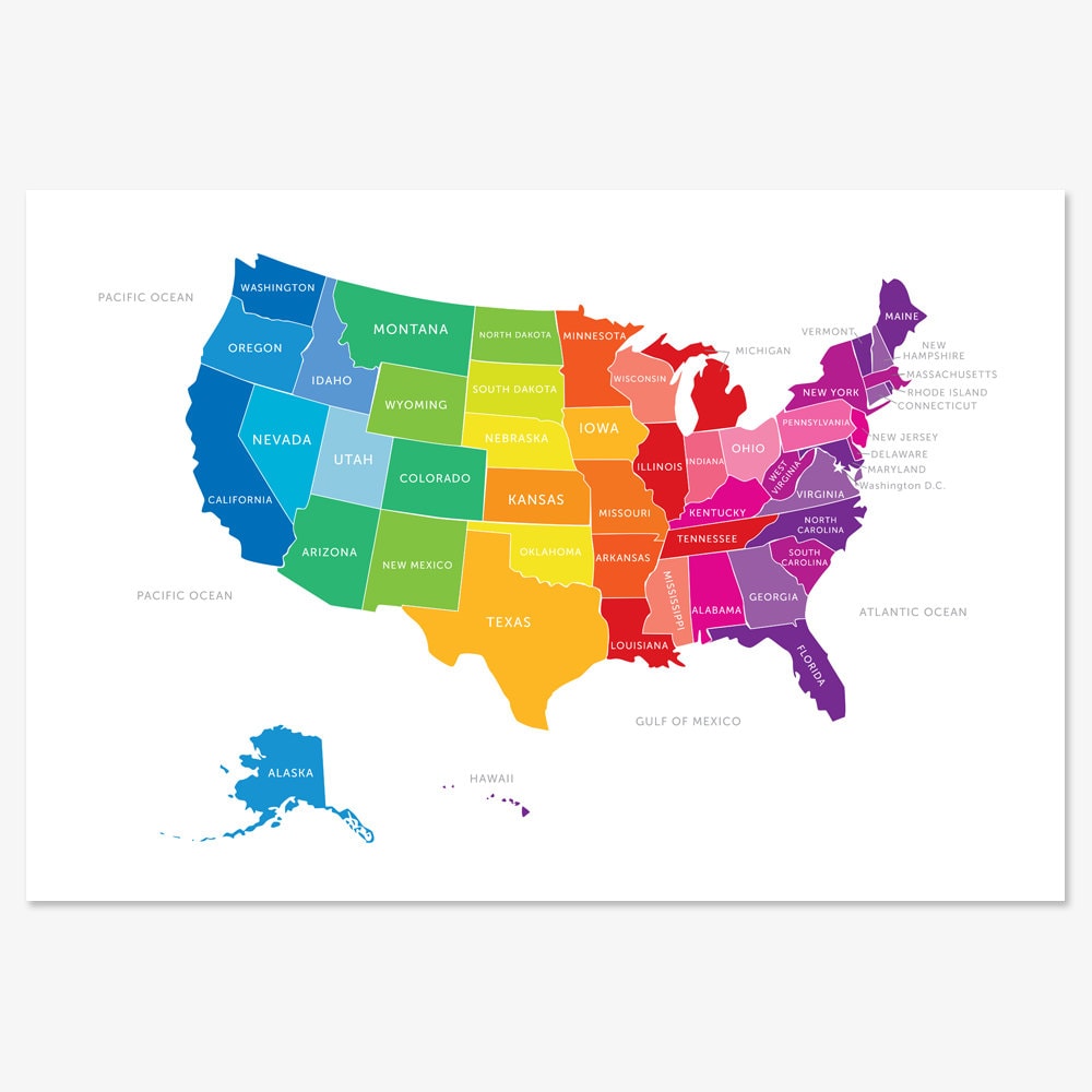
We associate the graph $G_{A}$ of the contiguous 48 States of America to the geographic map of the USA, by placing a vertex on every state, putting an edge between two vertices if the corresponding states share a border (at more than just a corner). We do not include vertices for Hawaii and Alaska, because, it is enought to compute $\chi(G,t)$ for its connected components $G_{j}$ to get $\chi(G,t)=\prod_{j}\chi(G_{j},t)$.

We attempted to calculate the chromatic polynomial for $G_{A}$. This was impossible to do entirely by hand, so we used modern computing technology to help with the calculations.

We tested different computing softwares, such as SAGE, Mathematica, MuPAD, and Maple. Each program was able to compute chromatic polynomials for relatively small graphs, but SAGE reached its limit when the number of vertices and edges was around 30 and 65 respectively. MuPAD couldn’t handle a similarly sized graph either. Given a 39-vertex, 83-edge graph, Maple ran unsuccessfully for over an hour, while Mathematica was able to handle it in just 4 minutes. Mathematica, however, couldn’t handle the entire $G_{A}$ with vertex-edge count of 48-105. From this, we knew our graph of the United States was too large for the best programs available to compute the chromatic polynomial. Because of its combinatorial nature, this is a problem of exponential complexity.

So, we combined the theory with our program of choice (Mathematica) to simplify our calculations.

Using the Chromatic Reduction Theorems, we were able to break down $G_{A}$ into subgraphs until it was reduced enough for Mathematica to compute the chromatic polynomials of these subgraphs. Using this approach, we calculated the chromatic polynomial of $G_{A}$ two different times in two different ways, each slightly differently.

In the first attempt, we consider $G_{A}$ an overlap of $W$ and graphs $N$, $Y$, and 3 $C_{3}$’s(cf. Figure 17). We let $N$ represent the northeastern-most states. We see that $Y$ overlaps $N$ and $W$, in $K_{1}$ and $K_{2}$ respectively. Each $C_{3}$ overlaps $W$ in $K_{2}$.

Figure 17: Attempt 1

Using CRT-1,

$$\chi(Y,t)=\frac{\chi(C_{3},t)^{3}}{\chi(K_{2},t)^{2}}.$$

We calculated $\chi(N,t)$ similarly.

Finally, by a repeated application of CRT-1, we get

$$\chi(G_{A},t)=\frac{\chi(W,t)\chi(Y,t)\chi(N,t)\chi(C_{3},t)^{3}}{\chi(K_{2},t)^{4}\chi(K_{1},t)}$$ (4)

Then using Mathematica to compute $\chi(W,t)$, and plugging it in (4), we get

$\chi(G_{A},t)=t^{48}-105t^{47}\newline +5404t^{46}-181689t^{45}\newline +4487296t^{44}-86797239t^{43}\newline +1369003119t^{42}-18100363324t^{41}\newline +204677484054t^{40}-2009741557171t^{39}\newline +17339117549604t^{38}-132682763002081t^{37}\newline +907423360476887t^{36}-5581169381630167t^{35}\newline +31031575427165032t^{34}-156643500973559120t^{33}\newline +720455907112532420t^{32}-3028205766124900090t^{31}\newline +11660587916045449786t^{30}-41218581559720380212t^{29}\newline +133971262465065322950t^{28}-400893632262902775367t^{27}\newline +1105490166090074304464t^{26}-2811013847987117591939t^{25}\newline +6593222714427581969721t^{24}-14265139633481475975539t^{23}\newline +28463416059570443463946t^{22}-52346700555134790196556t^{21}\newline +88655379811509518107152t^{20}-138105582619332483057236t^{19}\newline +197572598030181111248913t^{18}-259057209010976705704331t^{17}\newline +310574028340459418761423t^{16}-339434199963516594330980t^{15}\newline +336994442997740949240778t^{14}-302626296141859413511498t^{13}\newline +244548011549333689537938t^{12}-176716253459552869763068t^{11}\newline +113323961012010777670232t^{10}-63883998375551455822512t^{9}\newline +31284178773965469140544t^{8}-13106541029265128508800t^{7}\newline +4603738556785058047232t^{6}-1318612298697138044928t^{5}\newline +295742443634384435712t^{4}-48705983353199143936t^{3}\newline +5236695782665893888t^{2}-275716645154500608t$

Evaluating it at $t=4$ gives $\chi(G_{A},4)=12,811,729,152$. Thus,

the number of ways to color the map of the contiguous 48 states of America is

12,811,729,152

7 Conclusion

In Section 3, we listed some properties of the chromatic polynomial of a graph. We now use them to check our answer for $\chi(G_{A},t)$:

1. It is true that $\chi(G_{A},t)$ is monic, with integer coefficients.

2. The degree of $\chi(G_{A},t)$ is 48, the number of vertices in $G_{A}$.

3. The coefficient of $t^{47}$ is $-105$, the number of edges of $G_{A}$ is 105.

4. $G_{A}$ has no constant term, i.e. the constant term is zero.

5. The degree of the lowest term in $\chi(G_{A},t)$ is 1, which corresponds to the single component $G_{A}$ of the map of the contiguous 48 states of America.

6. The coefficients of $\chi(G_{A},t)$ clearly alternate between positive and negative.

7. As Mathematica verified, the sum of the coefficients of $G_{A}$ is indeed zero.

Thus, the polynomial we have found satisfies all of the above necessary conditions for a chromatic polynomial, and we are confident that our answer is correct.

For our second attempt, in order to double check the results of our first attempt, we consider $G_{A}$ an overlap of $X$ and $P$ in $K_{2}$, as pictured in Figure 18.

Figure 18: Attempt 2

We see that

$$\chi(G_{A},t)=\frac{\chi(X,t)\chi(P,t)}{\chi(K_{2},t)}$$

Surprisingly, Mathematica is able to compute the chromatic polynomial for X, a graph with 41 vertices and 93 edges. And of course, using methods previously discussed, $\chi(P,t)$ can be calculated by applying repeatedly the CRT - 1.

Again, it turns out that

$$\chi(G_{A},t)=\frac{\chi(X,t)\chi(P,t)}{\chi(K_{2},t)}=\frac{\chi(W,t)\chi(Y,t)\chi(N,t)\chi(C_{3},t)^{3}}{\chi(K_{2},t)^{4}\chi(K_{1},t)}$$

As expected, $\chi(G,t)=0$ for all $t\leq 3$. However,

$$\chi(G_{A},4)=12,811,591,729,152,$$

the number of ways to color $G_{A}$.

Remarks.
1. To color the entire map of the USA, multiply it with $4\cdot 4=16$ to include Alaska and Hawaii. If and when D.C becomes a state, the largest component $G_{A}$ of the map of the USA has to be enlarged and the new $\chi(G_{A},t)$ computed again.

References

• [1] F. Harary, Combinatorics, Addison-Wesley (1969).
• [2] R.C. Read, An Introduction to Chromatic Polynomials, J. Combinatorial Theory, 4(1968), 52–71.