Robust parametric modeling of Alzheimer’s disease progressionJournal: Journal of NeuroImage

Abstract

Quantitative characterization of disease progression using longitudinal data can provide long-term predictions for the pathological stages of individuals. This work studies robust modeling of Alzheimer’s disease progression using parametric methods. The proposed method linearly maps the individual’s chronological age to a disease progression score (DPS) and robustly fits a constrained generalized logistic function to the longitudinal dynamics of a biomarker as a function of the DPS using M-estimation. Robustness of the estimates is quantified using bootstrapping via Monte Carlo resampling, and the inflection points are used to temporally order the modeled biomarkers in the disease course. Moreover, kernel density estimation is applied to the obtained DPSs for clinical status prediction using a Bayesian classifier. Different M-estimators and logistic functions, including a new generalized type proposed in this study, called modified Stannard, are evaluated on the Alzheimer’s Disease Neuroimaging Initiative (ADNI) database for robust modeling of volumetric magnetic resonance imaging (MRI) and positron emission tomography (PET) biomarkers, as well as cognitive tests. The results show that the modified Stannard function fitted using the modified Huber loss achieves the best modeling performance with a mean absolute error (MAE) of $0.071$ across all biomarkers and bootstraps. In addition, applied to the ADNI test set, this model achieves a multi-class area under the ROC curve (AUC) of $0.87$ in clinical status prediction, and it significantly outperforms an analogous state-of-the-art method with a biomarker modeling MAE of $0.071$ vs. $0.073$ (Wilcoxon signed-rank test, $p<0.001$). Finally, the experiments show that the proposed model, trained using abundant ADNI data, generalizes well to data from the independent National Alzheimer’s Coordinating Center (NACC) database, where modeling performance is significantly improved (Wilcoxon signed-rank test, $p<0.001$) compared with using a model trained on relatively scarce NACC data.

1 Introduction

Figure 1: An illustration of the AD progression modeling method proposed by Jedynak et al. 2012; Jedynak et al. 2015. Left: A Sigmoid function is fitted to the biomarker measurements of each subject. Middle: The biomarker trajectories are aligned by linearly transforming the subjects’ ages to DPSs. Right: The aligned biomarker fit is obtained for all subjects.

Alzheimer’s disease (AD) is the most common type of dementia and leads to progressive neurodegeneration, affecting memory and behavior according to regional damage to brain cells (Ewers et al. 2011). The hippocampus, which is the center of learning and memory, is often one of the first regions of the brain to be damaged. It has also been shown that cerebrospinal fluid (CSF) biomarkers can become abnormal in the presymptomatic phase of the disease, preceding positron emission tomography (PET) and magnetic resonance imaging (MRI) biomarkers followed by clinical markers (Jack Jr et al. 2010; Biagioni and Galvin 2011). Currently, the cause of AD is not clear, and there is no cure or effective treatment to stop its progression, but an early diagnosis of the disease, especially in the pre-symptomatic stages, can provide time to treat symptoms and plan for the future. However, early diagnosis of AD is challenging mainly because elderly subjects under study can suffer from different age-related pathologies and normal aging besides AD. Therefore, methods to stage and identify at-risk individuals are critical to dementia research.

Disease progression modeling uses longitudinal studies to develop data-driven quantitative models that describe the evolution of the disease over time. The approach can therefore provide a complete perspective of the disease by computationally exploring the available data to help with better understanding of the disease for diagnostic, staging, monitorization, and prognostic purposes. Parametric disease progression modeling methods can be divided into two categories, continuous fitting for modeling the dynamic of biomarkers and discrete ordering for abnormality detection of biomarkers, both relying on unsupervised learning, e.g., by using maximum-likelihood estimation. The goal of the continuous approaches is to model biomarker values as a function of disease progression (Jedynak et al. 2012; Oxtoby and Alexander 2017). The discrete approaches, on the other hand, focus on temporally ordering of biomarkers becoming abnormal during the disease stages by discretizing the disease progression trajectory using generative, event-based models subjected to a number of assumptions (Fonteijn et al. 2012; Venkatraghavan et al. 2019).

Continuous, data-driven Alzheimer’s disease progression modeling has been inspired by the hypothetical models assuming sigmoidal evolution of AD biomarkers (Jack Jr et al. 2010; Jack Jr et al. 2013). Accordingly, a variety of approaches have been applied to fit a continuous function to the longitudinal dynamic of each biomarker using statistical models such as differential equations and mixed-effects models (Oxtoby et al. 2014; Yau et al. 2015; Guerrero et al. 2016), in which one needs to align the trajectory of individuals based on some time measure, e.g., time-to-conversion or years-to-onset. These methods are simple and require less data, but parametric assumptions on the biomarker trajectories limit the flexibility of the fits.

Recently, nonparametric disease progression modeling methods has been introduced to model biomarkers jointly while taking temporal dependencies among measurements into account (Lorenzi et al. 2017; Ghazi et al. 2019). These methods are flexible, make less assumption for modeling, and do not require alignment of the trajectories of the individuals. On the other hand, they are less interpretable, need a lot of multidimensional data for successful training, and cannot simply be applied to predict the test data when it includes missing or irregular visits, or when it has fewer biomarkers than what is used to train the network.

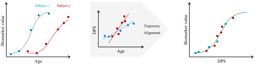
Jedynak et al. 2012; Jedynak et al. 2015 proposed a parametric algorithm, which requires less time-series data to train and incorporates information from multiple biomarkers for modeling progression of AD over a common disease timescale. As shown in Figure 1, the method linearly transforms the chronological age of individual to a disease progression score (DPS) for time-wise alignment of within-cohort measurements, assuming that the visit intervals in the data under study are short relative to the disease duration. Alternating least squares is used to fit a sigmoid function to the longitudinal dynamic of each biomarker. The model results in a reasonable approximation for normal or cognitively impaired subjects; however, it is not robust to outliers that can be found in a more contaminated data and does not generalize well for AD patients due to lack of data covering severe AD.

Figure 2: An illustration of how the proposed method (red curves) tackles the existing biomarker curve fitting problems. Left: A flexible function is used to better fit the asymmetric shape of the data points. Middle: A constrained function is utilized to estimate the exact dynamic of the biomarker considering its known lower and upper asymptotes. Right: A robust estimator is applied to fit a curve to data contaminated with outliers.

In this paper, a robust extension of Jedynak et al. 2012; Jedynak et al. 2015 is proposed that fits a constrained generalized logistic function to the longitudinal dynamic of each biomarker using M-estimation to address potential curve fitting problems in the biomarker modeling. Figure 2 illustrates 1) how the use of a generalized logistic function improves the curve flexibility, 2) how the use of a constrained function moves asymptotes to fit the exact dynamic of the biomarker, and 3) how the use of M-estimation reduces the influence of outliers. The estimated parameters are quantified using bootstrapping via Monte Carlo resampling, and the inflection points are used to temporally order the biomarkers in the disease course. In addition, kernel density estimation with normal bases is applied to the estimated DPSs for clinical status prediction using a Bayesian classifier. Different logistic functions, including a new generalized type proposed in this study called modified Stannard, and loss functions are applied to AD progression modeling of the Alzheimer’s Disease Neuroimaging Initiative (ADNI) (Petersen et al. 2010) and the National Alzheimer’s Coordinating Center (NACC) (Beekly et al. 2007) data using volumetric MRI biomarkers, PET measurements, and cognitive tests. The obtained results indicate that the proposed generalized logistic function (modified Stannard) fitted using the modified Huber loss achieves the best modeling performance over different bootstraps, and it consistently outperforms the basic algorithm of Jedynak et al. 2012; Jedynak et al. 2015 in all the considered experiments.

The main contribution of this study is four-fold. First, the introduction of different generalized logistic functions including the new type proposed in this study called modified Stannard allows for more flexibility, e.g., asymmetry, improving the biomarker trajectory modeling capabilities of the method compared to using a standard sigmoid function. Second, the use of M-estimation suppresses the effect of outliers on the fit. Third, the across-cohort generalizability of the proposed model is evaluated by applying the model trained using ADNI data to the test data from the NACC cohort. Finally, an end-to-end approach is introduced that performs biomarker trajectory modeling (unsupervised learning), biomarker’s significant change detection (event ordering), and clinical status prediction (supervised learning). This is a holistic way to implement a system suitable for both research and clinical applications to better study and monitor AD.

2 The proposed method

The main objective of this work is to minimize the error of parametric disease progression modeling while making the estimates stable and robust to outliers. This is achieved by fitting a constrained generalized logistic function using a maximum likelihood type estimator (M-estimator).

Table 1: Details of the utilized logistic functions for AD progression modeling. Note that the range of each function can be controlled by two additional parameters.

Logistic function	$g(s;\bm{\theta})$	$\bm{\theta}$	$(min,max)\,\forall\,b>0$	$g^{\prime}(s;\bm{\theta})$	$g^{\prime\prime}(c;\bm{\theta})$
Verhulst	$\left[1+e^{-b(s-c)}\right]^{-1}$	$\{b,c\}$	$(0,1)$ at $(-\infty,+\infty)$	$be^{-b(s-c)}\left[1+e^{-b(s-c)}\right]^{-2}$	0
Gompertz	$e^{-e^{-b(s-c)}}$	$\{b,c\}$	$(0,1)$ at $(-\infty,+\infty)$	$be^{-b(s-c)}e^{-e^{-b(s-c)}}$	0
Richards	$\left[1+\gamma e^{-b(s-c)}\right]^{-1/\gamma}$	$\{b,c,\gamma\}$	$(0,1)$ at $(-\infty,+\infty)$	$be^{-b(s-c)}\left[1+\gamma e^{-b(s-c)}\right]^{-1-1/\gamma}$	0
Modified Stannard	$\left[1+\frac{1}{\gamma}e^{-\frac{b}{\gamma}(s-c)}\right]^{-\gamma}$	$\{b,c,\gamma\}$	$(0,1)$ at $(-\infty,+\infty)$	$\frac{b}{\gamma}e^{-\frac{b}{\gamma}(s-c)}\left[1+\frac{1}{\gamma}e^{-\frac{b}{\gamma}(s-c)}\right]^{-1-\gamma}$	0

2.1 Modeling dynamics of biomarkers

Similar to Jedynak et al. 2012; Jedynak et al. 2015, two sets of parameters are estimated in the model: observed biomarker-specific parameters, which are assigned for fitting the biomarker curves, and hidden subject-specific (age-related) disease progression parameters that are defined for aligning the trajectory of subjects. Assume that $y_{i,j,k}$ is the $k$-th biomarker’s value at the $j$-th visit of the $i$-th subject and $f(s;\bm{\theta})$ is an S-shaped logistic function of DPS $s$ with parameters $\bm{\theta}$. Each biomarker measurement is defined as

$$y_{i,j,k}=f(s_{i,j};\bm{\theta}_{k})+\sigma_{k}\epsilon_{i,j,k}\,,$$

where $\sigma_{k}$ is the standard deviation of the $k$-th biomarker with $\bm{\theta}_{k}$ parameters, $\epsilon_{i,j,k}$ is additive white Gaussian noise (random effect) with i.i.d. assumption, and $s_{i,j}$ is the DPS for the $j$-th visit of the $i$-th subject and is obtained as

$$s_{i,j}=\alpha_{i}t_{i,j}+\beta_{i}\,,$$

where $t_{i,j}$ is the chronological age of subject $i$ in visit $j$, and $\alpha_{i}\in\mathbb{R}_{>0}$ and $\beta_{i}\in\mathbb{R}$ are the rate and onset of disease progression of subject $i$, respectively. Finally, the objective function for robust nonlinear regression is defined as

$$\{\hat{\bm{\alpha}},\hat{\bm{\beta}},\hat{\mathbf{\uptheta}},\hat{\bm{\sigma}}\}=\underset{i,j,k}{\min}\sum\limits_{i,j,k}\rho\left(\frac{y_{i,j,k}-f(\alpha_{i}t_{i,j}+\beta_{i};\bm{\theta}_{k})}{\sigma_{k}}\right)\,,$$

where $\rho(\cdot)$ is a maximum likelihood type function.

For fitting the longitudinal trajectories of biomarkers, four logistic functions are considered (Table 1). All functions have the same range $(0,1)$ and can produce the same inflection points at $c\in\mathbb{R}$, to be used for biomarker ordering. We candidate utilization of a flexible logistic function obtained by modifying Stannard function (Stannard et al. 1985) so as to create an asymmetric growth curve with an inflection point at $c$. In the defined functions, $b\in\mathbb{R}_{>0}$ and $\gamma\in\mathbb{R}_{>0}$ denote the growth rate and symmetry parameter of the curves, respectively. The reason for restricting $b$ to the positive real numbers is to make parameters of the estimation identifiable.

It can also be deducted from Table 1 that the sigmoid function first introduced by Verhulst (Verhulst 1845) is a special (symmetric) case of both Richards’ function (Richards 1959) and the proposed function when $\gamma=1$. Moreover, Gompertz’s function (Gompertz 1825) is a simplified form of Richards’ function when $\gamma$ approaches zero, i.e., $\lim_{\gamma\to 0}(1+\gamma u)^{-1/\gamma}=e^{-u}$. Finally, the upper and lower asymptotes of the curves can be adjusted by two additional parameters (Zwietering et al. 1990) as

$$f(s;\bm{\theta})=(a-d)g(s;\bm{\theta})+d\,.$$

The range parameters, $a$ and $d$, are set to fixed values corresponding to the pre-defined range of biomarkers. For those biomarkers whose exact range are not defined, e.g., volumetric MRI and PET measurements, the parameters are constrained to lower and upper bounds derived from the available range of the data, i.e., $lb\leq a,d\leq ub$.

2.2 Model fitting

Alternating approach, as an efficient optimization technique, is applied to solve the problem where the algorithm iteratively estimates $\mathbf{\uptheta}$ using fixed values of $\bm{\alpha}$ and $\bm{\beta}$ and vice versa until the parameters converge. This way, there is no need to optimize the objective function for the standard deviation of biomarkers $\sigma_{k}$, and they can be obtained when the biomarker-specific parameters are estimated. The proposed algorithm can be summarized as follows

1. Initialization: initialize $\{\bm{\alpha}^{(0)},\bm{\beta}^{(0)},\mathbf{\uptheta}^{(0)}\}$ and update them by iteratively applying linear least squares regression to fit the dynamics of biomarkers while linearly mapping ages to DPSs in an alternating scheme.

2. Optimization: iterate $l$ until convergence.

   Biomarker fitting: estimate the biomarker-specific parameters using values of all subjects and visits.

   $$\resizebox{17635710}{}{$\hat{\bm{\theta}}_{k}^{(l)}=\underset{(i,j)\in N_{k}}{\min}\sum\limits_{i,j}\rho\left(y_{i,j,k}-f(\hat{\alpha}_{i}^{(l-1)}t_{i,j}+\hat{\beta}_{i}^{(l-1)};\bm{\theta}_{k})\right)$}\,,$$ (1)

   $$\resizebox{17635710}{}{$\hat{\sigma}_{k}^{(l)}=\sqrt{\rule{0.0pt}{12.91663pt}\frac{1}{N_{k}-|\bm{\theta}_{k}|-2I_{k}}\sum\limits_{i,j}\rho\left(y_{i,j,k}-f(\hat{\alpha}_{i}^{(l-1)}t_{i,j}+\hat{\beta}_{i}^{(l-1)};\hat{\bm{\theta}}_{k}^{(l)})\right)}$}\,,$$

   Age mapping: estimate the subject-specific parameters using values of all biomarkers and visits.

   $$\resizebox{17635710}{}{$\{\hat{\alpha}_{i}^{(l)},\hat{\beta}_{i}^{(l)}\}=\underset{(j,k)\in N_{i}}{\min}\sum\limits_{j,k}\rho\left(\frac{y_{i,j,k}-f(\alpha_{i}t_{i,j}+\beta_{i};\hat{\bm{\theta}}_{k}^{(l)})}{\hat{\sigma}_{k}^{(l)}}\right)$}\,,$$ (2)

where $I_{k}$, $N_{k}$, and $N_{i}$ correspond to the number of subjects available for the $k$-th biomarker, number of measurements among all subjects and visits available for the $k$-th biomarker, and number of measurements among all biomarkers and visits available for the $i$-th subject, respectively. Moreover, $|\bm{\theta}_{k}|$ denotes the number of biomarker-specific parameters for the $k$-th biomarker, $\hat{\sigma}_{k}$ is called the generalized M-scale estimator (Van Aelst et al. 2013) for the $k$-th biomarker, and $N_{k}-|\bm{\theta}_{k}|-2I_{k}$ represents the degrees of freedom of the $k$-th fit. Therefore, the algorithm can be applied in case any subject has at least two distinct points considering all biomarkers and visits, and if any biomarker contains more than $|\bm{\theta}_{k}|+2I_{k}$ points considering all subjects and visits.

The utilized maximum likelihood type functions for robust regression (Holland and Welsch 1977; Pennacchi 2008) are described in Table 2. These estimators attempt to diminish influence of the outliers while fitting curves. In general, M-estimators use a tuning parameter called $\tau$ to scale the functions as $\tau^{2}\rho(r/\tau)$ in order to yield $95\%$ asymptotic efficiency with respect to the standard normal distribution. The corresponding tuning constants for the utilized functions are also reported in Table 2.

Table 2: The utilized $\rho$-type M-estimators and their corresponding scale factors $\tau$ for robust regression.

Loss function	$\rho(r)$	$\tau$
L2	$r^{2}$	1
L1-L2	$2\left(\sqrt{\rule{0.0pt}{7.74997pt}1+r^{2}}-1\right)$	1
Logistic	$\ln(\cosh(r))$	1.205
Modified Huber	$\begin{cases}1-\cos(\mathopen{|}r\mathclose{|}),&\mathopen{|}r\mathclose{|}\leq{\pi/2}\\ \mathopen{|}r\mathclose{|}+(1-\pi/2),&\mathopen{|}r\mathclose{|}>\pi/2\end{cases}$	1.2107
Cauchy-Lorentz	$\ln(1+r^{2})$	2.3849

Finally, the obtained DPSs are standardized with respect to the scores of the available cognitively normal visits of subjects in order to calibrate all biomarker trajectories in different experiments. This process removes mean of the normal visits’ distribution of DPSs and scales the range to give a better intuition of timing of disease progression in the course of AD. In this case, it would be necessary to properly update the parameters as

$$s_{i,j}=\left(s_{i,j}-\mu_{cn}\right)/\sigma_{cn}\,,$$

$$\alpha_{i}=\alpha_{i}/\sigma_{cn}\,,$$

$$\beta_{i}=\left(\beta_{i}-\mu_{cn}\right)/\sigma_{cn}\,,$$

$$b_{k}=\sigma_{cn}b_{k}\,,$$

$$c_{k}=\left(c_{k}-\mu_{cn}\right)/\sigma_{cn}\,,$$

where $\mu_{cn}$ and $\sigma_{cn}$ are the mean and standard deviation of the DPSs in the available cognitively normal visits of subjects, respectively.

2.3 Biomarker value prediction

Biomarker values can be predicted using the fitted model parameters. Age mapping part of the proposed algorithm is applied to estimate the subject-specific parameters using Equation (2) based on values of those biomarkers of the test subject that have available estimated biomarke-specific parameters in the fitted model. Next, biomarker values are predicted as $f(s_{i,j};\bm{\theta}_{k})$ using the estimated test DPSs where $f(\cdot)$ is the logistic function applied to model fitting.

2.4 Clinical status prediction

In order to predict the clinical status of test subjects per visit, kernel density estimation (KDE) (Parzen 1962) is used to fit likelihoods of cognitively normal, cognitively impaired, and AD groups in a nonparametric way. Assume that $(s_{1},s_{2},\ldots,s_{N})$ is a set of $N$ i.i.d. DPSs sampled from an unknown distribution with density function $p(s|c_{i})$, where $c_{i}$ denotes the $i$-th class label. KDE is expressed as

$$\hat{p}(s|c_{i})=\frac{1}{Nw}\sum\limits_{n=1}^{N}\mathscr{K}\left(\frac{s-s_{n}}{w}\right)\,,$$

where $\mathscr{K(\bm{\cdot})}$ is a smooth (kernel) function with a smoothing bandwidth $w>0$. Here, the Gaussian kernel is used as the smoothing function.

The clinical status is predicted based on the DPSs with a Bayesian classifier that uses the KDE-based fitted likelihoods as

$$p(c_{i}|s)=\frac{p(c_{i})p(s|c_{i})}{\sum\limits_{i}p(c_{i})p(s|c_{i})}\,,$$

where $p(c_{i})$ is the data-driven prior probability for the $i$-th class, the term in the denominator specifies the evidence, and $p(c_{i}|s)$ is the posterior probability for predicting the test DPS that belongs to the class $c_{i}$.

3 Experimental setup

3.1 Data

The data used in this work is obtained from the ADNI and the NACC databases.

3.1.1 ADNI

The ADNI was launched in 2003 as a public-private partnership, led by principal investigator Michael W. Weiner, MD. The primary goal of ADNI has been to test whether serial MRI, PET, other biological markers, and clinical and neuropsychological assessment can be combined to measure the progression of mild cognitive impairment and early Alzheimer’s disease. We use The Alzheimer’s Disease Prediction Of Longitudinal Evolution (TADPOLE) challenge dataset (Marinescu et al. 2018) that includes the three ADNI phases ADNI 1, ADNI GO, and ADNI 2. This dataset contains measurements from brain MRI, PET, CSF, cognitive tests, and demographics and genetics information.

The labels cognitively normal (CN), significant memory concern (SMC), and normal (NL) are merged under CN; mild cognitive impairment (MCI), early MCI (EMCI), and late MCI (LMCI) under MCI; and AD and dementia under AD. In addition, subjects converting from one clinical status to another, e.g., MCI-to-AD, are assigned the latter label (AD in this example). The utilized ADNI data includes T1-weighted brain MRI volumes of ventricles, hippocampus, whole brain, fusiform, and entorhinal cortex, fludeoxyglucose-PET (FDG-PET), as well as the cognitive tests clinical dementia rating sum of boxes (CDR-SB), Alzheimer’s disease assessment scale 13 items (ADAS-13), mini-mental state examination (MMSE), functional activities questionnaire (FAQ), Montreal cognitive assessment (MOCA), and Rey auditory verbal learning test of immediate recall (RAVLT-IR).

3.1.2 NACC

The NACC, established by the National Institute on Aging of the National Institutes of Health in 1999, has been developing a large database of standardized clinical and neuropathological data from both exploratory and explanatory Alzheimer’s disease research (Beekly et al. 2007). The data has been collected from different Alzheimer’s disease centers across the United States and among others contains measurements from different modalities such as MRI, PET, and cognitive tests.

Labels with numerical cognitive status of one (normal cognition) and two (impaired-not-MCI) are merged under CN, and cognitive status of three (MCI) and four (Dementia) are set to MCI and AD, respectively. It should be noted that we only keep subjects with primary etiologic diagnosis of normal, AD, or missing. This is to exclude subjects diagnosed with other types of dementia, non-neurodegenerative disease, or a non-neurological condition. The used NACC data includes T1-weighted brain MRI volumes of hippocampus and whole brain, and the cognitive tests MMSE, FAQ (sum of the 10-item scores), and CDR-SB using the CDR® Dementia Staging Instrument.

Table 3: Demographics of the utilized data across visits.

clinical status		age, year	education, year	MMSE
		(mean$\pm$SD)	(mean$\pm$SD)	(mean$\pm$SD)
	CN	77.81$\pm$4.95	15.55$\pm$3.03	29.11$\pm$1.09
	MCI	75.07$\pm$7.67	15.72$\pm$2.89	27.43$\pm$2.26
	AD	76.46$\pm$7.50	15.66$\pm$2.90	21.60$\pm$4.61
ADNI	Missing	74.30$\pm$7.97	15.97$\pm$2.74	26.06$\pm$3.79
	CN	81.86$\pm$7.72	13.92$\pm$3.58	27.93$\pm$2.10
	MCI	80.76$\pm$8.55	13.94$\pm$3.62	25.30$\pm$3.02
	AD	81.10$\pm$8.15	13.92$\pm$3.63	19.56$\pm$5.08
NACC	Missing	77.75$\pm$7.71	13.38$\pm$3.62

• Note that missing clinical status is indicated as ‘Missing’, and NACC subjects have no missing clinical status at visits with available cognitive tests including MMSE.

Table 4: Statistics of the visits per dataset.

	# visits per clinical status				# visits per subject	visit interval, year	# measurements per subject
	CN	MCI	AD	Missing	(mean$\pm$SD)	(mean$\pm$SD)	(mean$\pm$SD)
ADNI	405	3,846	2,057	528	5.76$\pm$2.42	0.73$\pm$0.41	48.49$\pm$21.56
NACC	178	204	317	85	6.76$\pm$2.67	1.13$\pm$0.53	19.66$\pm$7.40

3.1.3 Data filtering

In each of the ADNI and NACC datasets, the out-of-range measurements for the biomarkers with known range are rejected by assuming them as missing values. For the rest of the biomarkers, the most extreme outliers, which account for at most $1\%$ of the number of available within-class (clinical status) measurements across all subjects and visits, are detected by applying the generalized extreme Studentized deviate test (Rosner 1983) and are removed from each biomarker by assuming them as missing values.

Clinical follow-up visits with reverting clinical diagnoses are removed per subject considering the neighboring visits. In the ADNI dataset, clinical follow-up visits with wrongly ordered dates are discarded per subject. Also, MRI and PET measurements that are already matched to the cognitive visits with any extreme time gaps are excluded. The acceptable time gap is obtained based on the data statistics and is set to three months. In the NACC dataset, we perform the matching of MRI and clinical visits. However, due to the relative smaller sample size in NACC compared with ADNI, matches more than three months apart are kept and treated as two distinct visits. In this analysis, we assign a missing clinical status for any MRI visits that do not fall within the 3-month window.

In order to be able to apply the proposed method, measurements and clinical diagnoses with missing date information per visit are set to missing values, and subjects with less than two distinct visits are omitted. In addition, subjects with less than two available clinical diagnoses and removed. Finally, normal subjects staying normal are eliminated to reduce the effect of normal aging on AD progression modeling.

3.1.4 The obtained study population

After filtering the data, the utilized 12 ADNI biomarkers are acquired from 1,187 subjects (692 males and 495 females) in 6,836 visits between September 2005 and May 2017, and the five NACC biomarkers are acquired from 116 subjects (43 males and 73 females) in 784 visits between February 2002 and June 2018. Table 3 and Table 4 summarize statistics of the demographics and measurements in the two datasets after data filtering. Note that both datasets include missing values and missing clinical status, the latter indicated as ‘Missing’.

3.1.5 Data pre-processing

In the ADNI dataset, the volumetric measurements were obtained using two different versions of the public FreeSurfer software package (Fischl et al. 2002), and in the NACC dataset, they were calculated using IDeA Lab following ADNI protocols. Therefore, the MRI measurements need to be standardized across FreeSurfer version (Gronenschild et al. 2012) and across software package. In addition, biological difference in brain size hinders direct utilization of MRI measurements for disease progression estimation. Intracranial volume (ICV) is a commonly used measure for normalization to correct for head size. To overcome both aforementioned problems of difference in software (version) and head size, we employ the residual approach (O’Brien et al. 2011) based on the analysis of covariance, which takes data from control groups and linearly regresses MRI volumes on their corresponding ICV as a covariate of interest. The corrected measurements can thus be calculated as the estimated residuals $\hat{R}$ of the volumes using the regression parameters obtained from the control data as

$$\hat{R}_{i,j,k,v}=ROI_{i,j,k,v}-\left[\hat{\beta}_{k,v}^{cn}+\hat{\alpha}_{k,v}^{cn}ICV_{i,j,k,v}\right]\,,$$

where $ROI_{i,j,k,v}$ is the $k$-th MRI volume for subject $i$ at visit $j$ calculated (observed) using software or software version $v$, $ICV$ is the corresponding intracranial volume, and $\hat{\beta}^{cn}$ and $\hat{\alpha}^{cn}$ are the intercept and slope of the regression estimated from the CN group.

3.1.6 Data partitioning and bootstrapping

To evaluate the algorithms, each of the ADNI and NACC datasets is partitioned into two non-overlapping sets for training and testing. Based on the first and last available diagnoses of subjects, i.e., CN-CN, CN-MCI, …, AD-AD, we divide each of these types of pairs into two groups including few and large number of visits using the median number of visits as threshold and randomly select $15\%$ of the subjects from each of these groups for testing.

Additionally, bootstrapping is used in the experiments for quantification of the estimation, and in each bootstrap, a subset of the training subjects is randomly sampled with replacement based on the first and last available pair of diagnoses while ensuring that subjects with few and large number of visits are included in the training set. The unused subjects are assigned for validation, which constitute $1/e\approx 0.37$ of the subjects where $e$ is the base of the natural logarithm. This also means that the estimated variance using the bootstrapped model will account for approximately $63\%$ of the total variance.

To facilitate future research in AD progression modeling and comparison with the current study, all the data splits, including each bootstrap split, are also provided on arXiv as ancillary files.

3.2 Evaluation metrics

The mean absolute error (MAE) across all measurements is used to assess the modeling performance. It is a measure robust to outliers based on the absolute differences between actual and estimated values normalized by the range of the biomarkers as follows

$$\mathrm{MAE}=\frac{1}{I}\sum\limits_{i,j,k}\bigg|\frac{y_{i,j,k}-f(s_{i,j};\bm{\theta}_{k})}{ub_{k}-lb_{k}}\bigg|\,,$$

where $I$ is the total number of available measurements, $y_{i,j,k}$ and $f(s_{i,j};\bm{\theta}_{k})$ are the ground-truth and estimated values of the $k$-th biomarker for the $i$-th test subject at the $j$-th visit, and $lb_{k}$ and $ub_{k}$ indicate the lower and upper bounds of the $k$-th biomarker. The modeling performance of two different methods is statistically compared using the paired, two-sided Wilcoxon signed-rank test (Wilcoxon 1945) applied to the MAEs obtained from different bootstraps.

Additionally, multi-class area under the receiver operating characteristic (ROC) curve (AUC) (Hand and Till 2001) is used to measure the diagnostic performance in a multi-class test set and is calculated using the posterior probabilities as

$$\resizebox{22157625}{}{$\mathrm{AUC}=\frac{1}{(n_{c}(n_{c}-1))}\sum\limits_{i=1}^{n_{c}-1}\sum\limits_{k=i+1}^{n_{c}}\frac{1}{n_{i}n_{k}}\left[\mathrm{SR}_{i}-\frac{n_{i}(n_{i}+1)}{2}+\mathrm{SR}_{k}-\frac{n_{k}(n_{k}+1)}{2}\right]$}\,,$$

where $n_{c}$ is the number of distinct classes, $n_{i}$ denotes the number of available observations belonging to the $i$-th class, and $\mathrm{SR}_{i}$ is the sum of the ranks of posteriors $p(c_{i}|\bm{s}_{i})$ after sorting all concatenated posteriors $\{p(c_{i}|\bm{s}_{i}),p(c_{i}|\bm{s}_{k})\}$ in an ascending order, where $\bm{s}_{i}$ and $\bm{s}_{k}$ are vectors of DPSs belonging to the true classes $c_{i}$ and $c_{k}$, respectively. Likewise, $\mathrm{SR}_{k}$ is the sum of the ranks of posteriors $p(c_{k}|\bm{s}_{k})$ after sorting all concatenated posteriors $\{p(c_{k}|\bm{s}_{k}),p(c_{k}|\bm{s}_{i})\}$ in an ascending order.

Table 5: Modeling performance as MAE (mean$\pm$SD)$\times 10^{-3}$ for 100 bootstrapped ADNI validation subsets using different logistic and loss functions.

	L2	L1-L2	Logistic	Modified Huber	Cauchy-Lorentz
Verhulst	72.75$\pm$0.86	72.83$\pm$0.86	72.75$\pm$0.86	72.73$\pm$0.84	72.95$\pm$0.88
Gompertz	73.07$\pm$0.89	73.13$\pm$0.87	73.05$\pm$0.87	72.91$\pm$0.86	74.46$\pm$1.51
Richards	72.37$\pm$0.86	72.46$\pm$0.86	72.37$\pm$0.85	72.28$\pm$0.83	72.54$\pm$0.87
Modified Stannard	72.36$\pm$0.86	72.44$\pm$0.86	72.36$\pm$0.85	72.27$\pm$0.83	72.54$\pm$0.87

• The best result is shown in bold face and its corresponding configuration is selected for the remaining experiments.

3.3 Initialization of the algorithm and optimization

Since the fitting algorithm is iteratively performed using an alternating approach starting from values optimized in the previous step, initialization is an important step for efficiently reaching the optimum. We initially set $\bm{\alpha^{(0)}}$ and $\bm{\beta^{(0)}}$ to $\bm{1}$ and $\bm{0}$, respectively. Moreover, we set the intercept of the (substituted) linear functions used for biomarker fitting to $\bm{0}$ and their constrained slope ($\bm{\lambda}$) to either $-1$ or $1$ depending on the distribution of biomarker values across age. A positive slope is considered when the median of the $k$-th biomarker’s values for young subjects is less than that for old subjects and vice versa. Next, we update estimates of the subject/biomarker-specific parameters for $10$ iterations using linear least squares fitting for both biomarker fitting and age mapping.

After all parameters are linearly estimated, the parameters of the logistic functions are initially estimated as $\gamma_{k}=1$ and $b_{k}=4\lambda_{k}/(a_{k}-d_{k})$, where $d_{k}$ and $a_{k}$ are the minimum and maximum of the $k$-th biomarker’s values, respectively, provided that the slope $\lambda_{k}$ is positive, and vice versa if the slope is negative. In addition, each inflection point $c_{k}$ is estimated as the median of the obtained DPSs. Finally, we repeat the alternating procedure using the logistic functions and the trust-region algorithm (Coleman and Li 1996) considering robust estimators for at most $50$ iterations.

3.4 Stopping criteria

To avoid overfitting, the optimal parameter values are selected according to the optimum generalization loss obtained using the following criteria (Prechelt 1998)

$$\{\hat{\bm{\alpha}},\hat{\bm{\beta}},\hat{\mathbf{\uptheta}},\hat{\bm{\sigma}}\}=\min_{L_{min}\leq l\leq L_{max}}E_{valid}^{(l)}\,,$$

where $E_{valid}^{(l)}$ is the validation loss at the $l$-th iteration obtained through biomarker fitting using Equations (1) and (2). The minimum number of iterations, $L_{min}$, is set to $10$ to allow for enough training progress. The maximum number of iterations, $L_{max}$, is set to $50$. This avoids unnecessary computations since it was empirically observed that $E_{valid}$ attained a minimum well within this iteration range in all cases.

4 Results and discussion

4.1 Biomarker modeling

First, the proposed method is applied to model the dynamics of the ADNI biomarkers. Table 5 illustrates the modeling performance (MAE) for ADNI validation subsets obtained from 100 bootstraps using different logistic and loss functions. As can be seen, the combination of the modified Stannard function for biomarker fitting and the modified Huber loss achieves the best modeling performance of all the alternatives with both the lowest average MAE and the smallest standard deviation. This configuration will be used in all the remaining experiments.

To further investigate the stability and robustness of the model with the chosen configuration of logistic and loss functions, we visualize the fitted trajectories for each of the 100 bootstrap runs together with their average per biomarker in Figure 3.

Figure 3: Estimated curves per bootstrap (in gray) for the ADNI biomarkers using the modified Stannard function and the modified Huber loss. The average of the 100 bootstrapped curves per biomarker is shown as the black curve.

(a) The whole trajectory of all biomarkers.

(b) A zoom on the DPS axis showing the most dynamic area.

Figure 4: Average of the normalized curves of the ADNI biomarkers across 100 bootstraps.

Figure 5: Temporal ordering of the ADNI biomarkers in the disease course obtained using inflection points and quantified through 100 bootstraps.

4.2 Temporal ordering of biomarkers

To give an indication of the timing and the dynamics of the different biomarkers relative to each other, Figure 4 shows the average curves scaled to $[0,1]$ using the estimated upper and lower asymptotes per biomarker and superimposed in the same figure. The distribution of the inflection points of the biomarkers, quantified through bootstrapping, can be used to see how biomarkers proceed in the course of AD with respect to each other. The inflection point can be considered a turning point after which a dramatic change in the biomarker is expected to occur. Figure 5 displays the temporal ordering of the ADNI biomarkers based on the estimated inflection points. As can be seen, RAVLT-IR precedes all other biomarkers. This interesting finding is in line with the results of Jedynak et al. 2012; Jedynak et al. 2015; Young et al. 2015 and is consistent with several clinical studies concluding that some cognitive tests including RAVLT are significant predictors that can predict neurodegenerative changes up to 10 years before clinical diagnosis (Tierney et al. 2005; Landau et al. 2010; Zandifar et al. 2019). Moreover, bearing Figure 4 in mind, volumetric MRI biomarkers start becoming abnormal early in the disease course. However, some of these biomarkers such as ventricles and whole brain are, as also seen in Figure 5, noisy measurements to model progression of AD in this dataset. It is important to note that the inflection points are utilized to order the biomarkers in the disease course. These points do not imply when the biomarkers start becoming abnormal and hence, are not measures for early abnormality detection.

4.3 DPS distribution versus biomarker timing

Figure 6 shows the variance of the estimated inflection points per biomarker alongside the estimated class-conditional likelihoods of the obtained DPSs from 100 bootstraps. As can be seen, there is a high overlap between the DPS distributions of CN and MCI while the CN and AD groups can be discriminated easily. Moreover, the estimated inflection points per biomarker are almost in line with those of the hypothetical model by Jack Jr et al. 2010 that illustrates when biomarkers are dynamic versus disease stages. Especially, inflection points of the MRI biomarkers (brain structure) are mainly located in the MCI stage while those of the cognitive tests (memory) lie on the AD stage.

Table 6: Test modeling performance of different methods as MAE (mean$\pm$SD)$\times 10^{-3}$ for ADNI and NACC test biomarkers. All average MAEs are significantly different ($p<0.001$).

	Within cohort		Across cohort
Method	ADNI	NACC	ADNI to NACC
Jedynak et al. 2015	72.59$\pm$0.59	79.98$\pm$4.39	78.97$\pm$0.95
The proposed method	71.42$\pm$0.26	74.35$\pm$4.36	73.41$\pm$1.10

4.4 Predicting biomarker values

The biomarker-specific parameters estimated using the training set in each bootstrap are applied to map the test individuals’ ages to DPSs using Equation (2). The obtained DPSs are subsequently fed to the per-bootstrap estimated biomarker functions for the proposed model and the analogous state-of-the-art model by Jedynak et al. 2015 that fits the basic sigmoid function using unconstrained, L2-norm loss function to evaluate their predictive power. Table 6 shows the ADNI test MAEs of the aforementioned methods obtained using the estimates from 100 bootstraps. The proposed model significantly outperforms the analogous state-of-the-art model with an average MAE of $0.071$ vs. $0.073$ ($p<0.001$).

Figure 6: Estimated class-conditional likelihoods using the DPSs obtained from 100 ADNI-trained bootstraps. The box plots indicate the 25th to 75th percentiles of the estimated inflection points per biomarker, centrally marked with the median, and they are extended to the most extreme non-outlier inflection points using dashed lines.

Figure 7: Estimated curves per bootstrap (in gray) for the NACC biomarkers using the modified Stannard function and the modified Huber loss. The average of the 100 bootstrapped curves per biomarker is shown as the black curve. The last subfigure shows average of the normalized curves of the NACC biomarkers across 100 bootstraps.

4.5 Predicting clinical status

To evaluate the diagnostic predictive performance, the obtained training DPSs per bootstrap are used to estimate class-conditional likelihood functions using KDE and fed to a three-class Bayesian classifier with prior probabilities proportional to the number of training observations in each class. The classifiers, one for each bootstrap, are applied to the test DPSs estimated as described in Section 4.4 to compute the posterior probabilities of the clinical labels. The proposed model achieves an AUC of $0.86\pm 0.01$ in predicting the clinical status of the test ADNI subjects per visit, which reveals the effect of modeling on classification performance.

The obtained posterior probabilities from the different classifiers from each bootstrap can be combined using ensemble learning techniques to potentially improve prediction performance and robustness (Kuncheva 2014); for example, by taking the average of the within-class posteriors over an ensemble of models from different bootstraps, corresponding to bagging, before calculating the AUC. By fusing the posteriors of the proposed method in such a way, the AUC increases to $0.87$.

The AUC of $0.87$ obtained using the proposed method outperforms the state-of-the-art, cross-sectional MRI-based classification results of the challenge on Computer-Aided Diagnosis of Dementia (CADDementia) (Bron et al. 2015) where the best AUC was $0.79$. However, it should be noted that the CADDementia algorithms were applied to classify data from independent cohorts using different types of cross-sectional MRI biomarkers besides volumetry.

4.6 Generalizability across cohorts

As the final set of experiments, the generalizability of the proposed model to an independent cohort is assessed using the NACC data. First, the model using the optimal configuration (modified Stannard as logistic function and modified Huber loss as M-estimator) according to the ADNI experiments is applied to model AD within NACC. Figure 7 depicts the modeled NACC biomarkers for 100 bootstraps. Second, the previously ADNI-trained model with the optimal configuration is utilized to predict the NACC test measurements using the ADNI-based estimates of the corresponding set of biomarkers, i.e., CDR-SB, MMSE, FAQ, hippocampus, and whole brain. Table 6 compares the modeling performance of the ADNI-trained and the NACC-trained models applied to the NACC test set. As it can be noticed from the obtained results, the previously selected configuration for ADNI data is also a good choice when applied to NACC data. Moreover, both modeling performance of the proposed method and the state-of-the-art model of Jedynak et al. 2015 significantly improve ($p<0.001$) when applying the ADNI-trained model to the NACC test set by average MAEs of $0.0009$ and $0.0010$, respectively. That is, not only does the ADNI-trained model generalize across cohorts, it also improves the performance compared to using the NACC-trained model. One reason for the improvement could be the relatively larger size of the ADNI data and its additional biomarkers providing a better foundation for robust modeling of biomarkers. The results also show that the proposed model significantly outperforms ($p<0.001$) the state-of-the-art model of Jedynak et al. 2015 in all cases.

Additionally, we apply the ADNI and NACC trained classifiers to the estimated test NACC DPSs to predict the clinical status per subject per visit. The proposed method achieves AUCs of $0.92\pm 0.05$ and $0.93\pm 0.06$, respectively. This reveals that the diagnostic performance improves when applying the ADNI-trained model to the NACC test set.

5 Conclusions

In this paper, a robust parametric model of Alzheimer’s disease progression was proposed based on alternating M-estimation using the modified Huber loss that linearly transformed individuals’ chronological ages to disease progression scores and fitted a novel generalized logistic function to the longitudinal dynamic of each biomarker. The estimated parameters were then used to temporally order the biomarkers in the disease course and to predict the test biomarker values as well as the clinical status per subject visit. The obtained results showed the superiority of the proposed method over the analogous state-of-the-art model proposed by Jedynak et al. 2015 in terms of prediction performance and generalizability.

The proposed approach can be applied to different time-series data including missing points and labels, or to biomarkers with other characteristics than the monotonic behavior that one typically encounters in MRI-based neurodegenerative disease progression modeling as long as suitable functions are used for the biomarker modeling. Moreover, as an alternative to using M-estimators, resistant estimators such as the least trimmed sum of squares and least median of squares (Rousseeuw and Leroy 1987) with higher breakdown points can be used instead in the algorithm to fit biomarkers. However, this will result in an additional parameter to be optimized for the coverage (range) needed for trimming the residuals.

Disclosures

M. Nielsen is shareholder in Biomediq A/S and Cerebriu A/S. A. Pai is shareholder in Cerebriu A/S. The remaining authors report no disclosures.

References

- Beekly et al. (2007) Beekly, D.L., Ramos, E.M., Lee, W.W., Deitrich, W.D., Jacka, M.E., Wu, J., Hubbard, J.L., Koepsell, T.D., Morris, J.C., Kukull, W.A., et al., 2007. The National Alzheimer’s Coordinating Center (NACC) database: the uniform data set. Alzheimer Dis. Assoc. Disord. 21, 249–258.
- Biagioni and Galvin (2011) Biagioni, M.C., Galvin, J.E., 2011. Using biomarkers to improve detection of Alzheimer’s disease. Neurodegener. Dis. Manag. 1, 127–139.
- Bron et al. (2015) Bron, E.E., Smits, M., Van Der Flier, W.M., Vrenken, H., Barkhof, F., Scheltens, P., Papma, J.M., Steketee, R.M., Orellana, C.M., Meijboom, R., et al., 2015. Standardized evaluation of algorithms for computer-aided diagnosis of dementia based on structural MRI: the CADDementia challenge. NeuroImage 111, 562–579.
- Coleman and Li (1996) Coleman, T.F., Li, Y., 1996. An interior trust region approach for nonlinear minimization subject to bounds. SIAM J. Optim. 6, 418–445.
- Ewers et al. (2011) Ewers, M., Sperling, R.A., Klunk, W.E., Weiner, M.W., Hampel, H., 2011. Neuroimaging markers for the prediction and early diagnosis of Alzheimer’s disease dementia. Trends Neurosci. 34, 430–442.
- Fischl et al. (2002) Fischl, B., Salat, D.H., Busa, E., Albert, M., Dieterich, M., Haselgrove, C., Van Der Kouwe, A., Killiany, R., Kennedy, D., Klaveness, S., Montillo, A., Makris, N., Rosen, B., Dale, A.M., 2002. Whole brain segmentation: automated labeling of neuroanatomical structures in the human brain. Neuron 33, 341–355.
- Fonteijn et al. (2012) Fonteijn, H.M., Modat, M., Clarkson, M.J., Barnes, J., Lehmann, M., Hobbs, N.Z., Scahill, R.I., Tabrizi, S.J., Ourselin, S., Fox, N.C., et al., 2012. An event-based model for disease progression and its application in familial Alzheimer’s disease and Huntington’s disease. NeuroImage 60, 1880–1889.
- Ghazi et al. (2019) Ghazi, M.M., Nielsen, M., Pai, A., Cardoso, M.J., Modat, M., Ourselin, S., Sørensen, L., 2019. Training recurrent neural networks robust to incomplete data: application to Alzheimer’s disease progression modeling. Med. Image Anal. 53, 39–46.
- Gompertz (1825) Gompertz, B., 1825. On the nature of the function expressive of the law of human mortality, and on a new mode of determining the value of life contingencies. Philos. Trans. R. Soc. London , 513–583.
- Gronenschild et al. (2012) Gronenschild, E.H., Habets, P., Jacobs, H.I., Mengelers, R., Rozendaal, N., Van Os, J., Marcelis, M., 2012. The effects of FreeSurfer version, workstation type, and Macintosh operating system version on anatomical volume and cortical thickness measurements. PloS One 7, e38234.
- Guerrero et al. (2016) Guerrero, R., Schmidt-Richberg, A., Ledig, C., Tong, T., Wolz, R., Rueckert, D., 2016. Instantiated mixed effects modeling of Alzheimer’s disease markers. NeuroImage 142, 113–125.
- Hand and Till (2001) Hand, D.J., Till, R.J., 2001. A simple generalisation of the area under the ROC curve for multiple class classification problems. Mach. Learn. 45, 171–186.
- Holland and Welsch (1977) Holland, P.W., Welsch, R.E., 1977. Robust regression using iteratively reweighted least-squares. Commun. Stat. Theory Methods 6, 813–827.
- Jack Jr et al. (2013) Jack Jr, C.R., Knopman, D.S., Jagust, W.J., Petersen, R.C., Weiner, M.W., Aisen, P.S., Shaw, L.M., Vemuri, P., Wiste, H.J., Weigand, S.D., et al., 2013. Tracking pathophysiological processes in Alzheimer’s disease: an updated hypothetical model of dynamic biomarkers. Lancet Neurol. 12, 207–216.
- Jack Jr et al. (2010) Jack Jr, C.R., Knopman, D.S., Jagust, W.J., Shaw, L.M., Aisen, P.S., Weiner, M.W., Petersen, R.C., Trojanowski, J.Q., 2010. Hypothetical model of dynamic biomarkers of the Alzheimer’s pathological cascade. Lancet Neurol. 9, 119–128.
- Jedynak et al. (2012) Jedynak, B.M., Lang, A., Liu, B., Katz, E., Zhang, Y., Wyman, B.T., Raunig, D., Jedynak, C.P., Caffo, B., Prince, J.L., 2012. A computational neurodegenerative disease progression score: method and results with the Alzheimer’s Disease Neuroimaging Initiative cohort. NeuroImage 63, 1478–1486.
- Jedynak et al. (2015) Jedynak, B.M., Liu, B., Lang, A., Gel, Y., Prince, J.L., 2015. A computational method for computing an Alzheimer’s disease progression score; experiments and validation with the ADNI data set. Neurobiol. Aging 36, S178–S184.
- Kuncheva (2014) Kuncheva, L.I., 2014. Combining pattern classifiers: methods and algorithms. John Wiley & Sons.
- Landau et al. (2010) Landau, S., Harvey, D., Madison, C., Reiman, E., Foster, N., Aisen, P., Petersen, R.C., Shaw, L., Trojanowski, J., Jack, C., et al., 2010. Comparing predictors of conversion and decline in mild cognitive impairment. Neurol. 75, 230–238.
- Lorenzi et al. (2017) Lorenzi, M., Filippone, M., Frisoni, G.B., Alexander, D.C., Ourselin, S., 2017. Probabilistic disease progression modeling to characterize diagnostic uncertainty: application to staging and prediction in Alzheimer’s disease. NeuroImage 190, 56–68.
- Marinescu et al. (2018) Marinescu, R.V., Oxtoby, N.P., Young, A.L., Bron, E.E., Toga, A.W., Weiner, M.W., Barkhof, F., Fox, N.C., Klein, S., Alexander, D.C., 2018. TADPOLE challenge: prediction of longitudinal evolution in Alzheimer’s disease. CoRR abs/1805.03909.
- O’Brien et al. (2011) O’Brien, L.M., Ziegler, D.A., Deutsch, C.K., Frazier, J.A., Herbert, M.R., Locascio, J.J., 2011. Statistical adjustments for brain size in volumetric neuroimaging studies: some practical implications in methods. Psychiatry Res.: Neuroimaging 193, 113–122.
- Oxtoby and Alexander (2017) Oxtoby, N.P., Alexander, D.C., 2017. Imaging plus X: multimodal models of neurodegenerative disease. Curr. Opin. Neurol. 30, 371.
- Oxtoby et al. (2014) Oxtoby, N.P., Young, A.L., Fox, N.C., Daga, P., Cash, D.M., Ourselin, S., Schott, J.M., Alexander, D.C., 2014. Learning imaging biomarker trajectories from noisy Alzheimer’s disease data using a Bayesian multilevel model, in: Bayesian and Graphical Models for Biomedical Imaging, pp. 85–94.
- Parzen (1962) Parzen, E., 1962. On estimation of a probability density function and mode. Ann. Math. Stat. 33, 1065–1076.
- Pennacchi (2008) Pennacchi, P., 2008. Robust estimate of excitations in mechanical systems using M-estimators–theoretical background and numerical applications. J. Sound Vib. 310, 923–946.
- Petersen et al. (2010) Petersen, R.C., Aisen, P., Beckett, L., Donohue, M., Gamst, A., Harvey, D., Jack, C., Jagust, W., Shaw, L., Toga, A., Trojanowski, J., Weiner, M., 2010. Alzheimer’s Disease Neuroimaging Initiative (ADNI): clinical characterization. Neurol. 74, 201–209.
- Prechelt (1998) Prechelt, L., 1998. Early stopping–but when?, in: Neural Networks: Tricks of the Trade, pp. 55–69.
- Richards (1959) Richards, F., 1959. A flexible growth function for empirical use. J. Exp. Bot. 10, 290–301.
- Rosner (1983) Rosner, B., 1983. Percentage points for a generalized ESD many-outlier procedure. Technometrics 25, 165–172.
- Rousseeuw and Leroy (1987) Rousseeuw, P.J., Leroy, A.M., 1987. Robust regression and outlier detection. volume 1. Wiley Online Library.
- Stannard et al. (1985) Stannard, C., Williams, A., Gibbs, P., 1985. Temperature/growth relationships for psychrotrophic food-spoilage bacteria. Food Microbiol. 2, 115–122.
- Tierney et al. (2005) Tierney, M.C., Yao, C., Kiss, A., McDowell, I., 2005. Neuropsychological tests accurately predict incident Alzheimer disease after 5 and 10 years. Neurol. 64, 1853–1859.
- Van Aelst et al. (2013) Van Aelst, S., Willems, G., Zamar, R.H., 2013. Robust and efficient estimation of the residual scale in linear regression. J. Multivar. Anal. 116, 278–296.
- Venkatraghavan et al. (2019) Venkatraghavan, V., Bron, E.E., Niessen, W.J., Klein, S., 2019. Disease progression timeline estimation for Alzheimer’s disease using discriminative event based modeling. NeuroImage 186, 518–532.
- Verhulst (1845) Verhulst, P., 1845. La loi d’accroissement de la population. Nouv. Mém. de l’Academie Royale des Sci. et Belles-Lettres de Bruxelles 18, 1–41.
- Wilcoxon (1945) Wilcoxon, F., 1945. Individual comparisons by ranking methods. Biom. Bull. 1, 80–83.
- Yau et al. (2015) Yau, W.Y.W., Tudorascu, D.L., McDade, E.M., Ikonomovic, S., James, J.A., Minhas, D., Mowrey, W., Sheu, L.K., Snitz, B.E., Weissfeld, L., et al., 2015. Longitudinal assessment of neuroimaging and clinical markers in autosomal dominant Alzheimer’s disease: a prospective cohort study. Lancet Neurol. 14, 804–813.
- Young et al. (2015) Young, A.L., Oxtoby, N.P., Huang, J., Marinescu, R.V., Daga, P., Cash, D.M., Fox, N.C., Ourselin, S., Schott, J.M., Alexander, D.C., 2015. Multiple orderings of events in disease progression, in: International Conference on Information Processing in Medical Imaging, pp. 711–722.
- Zandifar et al. (2019) Zandifar, A., Fonov, V., Ducharme, S., Belleville, S., Collins, D.L., 2019. MRI and cognitive scores complement each other to accurately predict Alzheimer’s dementia 2 to 7 years before clinical onset. bioRxiv , 567867.
- Zwietering et al. (1990) Zwietering, M., Jongenburger, I., Rombouts, F., Van’t Riet, K., 1990. Modeling of the bacterial growth curve. Appl. Environ. Microbiol. 56, 1875–1881.