R-miss-tastic: a unified platform for missing values methods and workflows

Abstract

Missing values are unavoidable when working with data. Their occurrence is exacerbated as more data from different sources become available. However, most statistical models and visualization methods require complete data, and improper handling of missing data results in information loss, or biased analyses. Since the seminal work of Rubin 1976, there has been a burgeoning literature on missing values with heterogeneous aims and motivations. This has resulted in the development of various methods, formalizations, and tools (including a large number of R packages and Python modules). However, for practitioners, it remains challenging to decide which method is most suited for their problem, partially because handling missing data is still not a topic systematically covered in statistics or data science curricula.

To help address this challenge, we have launched a unified platform: “R-miss-tastic”, which aims to provide an overview of standard missing values problems, methods, how to handle them in analyses, and relevant implementations of methodologies. In the same perspective, we have also developed several pipelines in R and Python to allow for a hands-on illustration of how to handle missing values in various statistical tasks such as estimation and prediction, while ensuring reproducibility of the analyses. This will hopefully also provide some guidance on deciding which method to choose for a specific problem and data. The objective of this work is not only to comprehensively organize materials, but also to create standardized analysis workflows, and to provide a common ground for discussions among the community. This platform is thus suited for beginners, students, more advanced analysts and researchers.

Keywords: missing data; state of the art; bibliography; reproducibility; guided workflows; teaching material

1 Context and motivation

Missing data are unavoidable as soon as collecting or acquiring data is involved. They occur for many reasons including: individuals choose not to answer survey questions, measurement devices fail, or data have simply not been recorded. Their presence becomes even more important as data are now obtained at increasing velocity and volume, and from heterogeneous sources not originally designed to be analyzed together. As pointed out by Zhu et al. 2019, “one of the ironies of working with Big Data is that missing data play an ever more significant role, and often present serious difficulties for analysis”. Despite this, the approach most commonly implemented by default in software is to toss out cases with missing values. At best, this is inefficient because it wastes information from the partially observed cases. At worst, it results in biased estimates, particularly when the distributions of the missing values are systematically different from those of the observed values (e.g., Enders 2010, Chap. 2).

However, handling missing data in a more efficient and relevant way (than limiting the analysis on solely the complete cases) has attracted a lot of attention in the literature in the last two decades. In particular, a number of reference books have been published (Schafer and Graham 2002; Little and Rubin 2002; van Buuren 2012; Carpenter and Kenward 2012) and the topic is an active field of research (Josse and Reiter 2018). The diversity of the problems of missing data means there is great variety in the methods proposed and studied. They include model-based approaches, integrating likelihoods or posterior distributions over missing values, filling in missing values in a realistic way with single, or multiple imputations, or weighting approaches, appealing to ideas from the design-based literature in survey sampling. The multiplicity of the available solutions makes sense because there is no single solution or tool to manage missing data: the appropriate methodology to handle them depends on many features, such as the objective of the analysis, type of data, the type of missing data and their pattern. Some of these methods are available in various and heterogeneous software solutions. As R (R Core Team 2020) is one of the main softwares for statisticians and data scientists and as its development has started almost three decades ago (Ihaka 1998), R is one of the language that offers the largest number of implemented approaches. This is also due to its ease to incorporate new methods and its modular packaging system. Currently, there are over 270 R packages on CRAN that mention missing data or imputation in their DESCRIPTION files. These packages serve many different applications, data types or types of analysis. More precisely, exploratory and visualization tools for missing data are available in packages like naniar, VIM, and MissingDataGUI (Tierney et al.; Tierney and Cook 2018; Kowarik and Templ 2016; Cheng et al. 2015). Imputation methods are included in packages like mice, Amelia, and mi (van Buuren and Groothuis-Oudshoorn 2011; Honaker et al. 2011; Gelman and Hill 2011). Other packages focus on dealing with complex, heterogeneous (categorical, quantitative, ordinal variables) data or with large dimension multi-level data, such as missMDA, and MixedDataImpute (Josse et al. 2016; Murray and Reiter 2015). To our knowledge, R is the programming language offering the largest variety of implemented methods. However, other languages such as Python (Van Rossum and Drake 2009), which currently only have few publicly available implementations of methods that handle missing values in statistical tasks, offer more and more solutions. Two prominent examples are: 1) the scikit-learn library (Pedregosa et al. 2011) which has recently added a module for missing values imputation; and 2) the DataWig library (Biessmann et al. 2018) which provides a framework to learn to impute incomplete data tables.

The rich variety of methods and tools for working with missing data means there are many solutions for a variety of applications. Despite the number of options, missing data are often not handled appropriately by practitioners. This may be for a few reasons. First, the plethora of options can be a double-edged sword - the sheer number of options making it challenging to navigate and find the best one. Second, the topic of missing data is often itself missing from many statistics and data science syllabuses, despite its relative omnipresence in data. So then, faced with missing data, practitioners are left powerless: quite possibly never having been taught about missing data, they do not have an idea of how to approach the problem, what are the dangers of mismanagement, navigate the methods, software, or choose the appropriate method or workflow for their problem.

To help promote better management and understanding of missing data, we have released R-miss-tastic, an open platform for missing values. The platform takes the form of a reference website, which collects, organizes and produces material on missing data. It has been conceived by an infrastructure steering committee (ISC; its members are authors of this article) working group, which first provided a CRAN Task View on missing data that lists and organizes existing R packages on the topic. The “R-miss-tastic” platform extends and builds on the CRAN Task View by collecting and organizing articles, tutorials, documentation, and workflows for analyses with missing data. The platform provides new tutorials, examples and pipelines of analyses we have developed with missing data that span the entirety of an analysis. The latter have been developed by us and implemented in R and in Python for this platform, implementing standard methods for generating missing values and analyzing them under different perspectives. Starting from data preparation, these pipelines also cover exploratory data analyses, establishing statistical models, analysis diagnostics, applying machine learning methods, through to communication of the results obtained from incomplete data. We hope that these pipelines also serve as guidance when it comes to choosing a method to handle missing values in a specific context.

Another important ingredient in statistical analyses, some may even argue the most important one, is data which a proposed method or estimator is apply to. We thus also reference publicly available datasets that are commonly used as benchmark for new missing values methodologies. It is easily extendable and well documented, so it can seamlessly incorporate future research in missing values. The intent of the platform is to foster a welcoming community, within and beyond the R community . “R-miss-tastic” has been designed to be accessible for a wide audience with different levels of prior knowledge, needs, and questions. This includes, for instance, students looking for course material to complement their studies, teachers and professors who can use a reference website for their own classes or refer to students, statisticians or researchers in a different fields using statistics searching for solutions or existing work to help with analysis, researchers wishing to understand or contribute information for specific research questions, or find collaborators.

The remainder of the article is organized as follows: Section 2 describes the different components of the platform, the structure that has been chosen, and the targeted audience. The section is organized as the platform itself, starting by describing materials for less advanced users then materials for researchers and finally resources for practical implementation. Section 3 details the implementation and use-cases of the provided workflows, implemented both in R and in Python. Finally, in Section 4 we conclude with an overview of the planed future development for the platform and of interesting areas in missing values research that we would like to bring to a broader audience.

2 Structure and content of the platform

The R-miss-tastic platform is released at https://rmisstastic.netlify.com/. It has been developed using the R package blogdown Xie et al. 2017 which wraps hugo. Live examples have been included using the tool https://rdrr.io/snippets/ provided by the website ‘‘R Package Documentation’’. The source code and materials of the platform have been made publicly available on GitHub, which provides a transparent record of the platform’s development, and facilitates community contributions.

We now discuss the structure of the R-miss-tastic platform, the aim and content of each subsection, and highlight key features of the platform.

2.1 Workflows

An important contribution and novelty of this work is the proposal of several workflows that allow for a hands-on illustration of classical analyses with missing values, both on simulated data and on publicly available real-world data. These workflows are provided both in R and in Python code and cover the following topics:

• How to generate missing values? Generate missing values under different mechanisms, on complete or incomplete datasets. This is useful when performing simulations to compare methods.

• How to do statistical inference with missing values? We focus in particular in the different solutions (maximum likelihood or multiple imputation) that are available to estimate linear and logistic regression parameters with missing values in the covariates.

• How to impute missing values? We compare different single imputation/matrix completion methods (for instance using conditional models, low-rank models, etc.)

• How to predict with missing values? We consider establishing predictive models (for instance using random forests (Breiman 2001)) on data with incomplete predictors. The workflows present different strategies to deal with the missing values in the covariates both in the train set and in the test set.

The aim of these workflows is threefold: 1) they provide a practical implementation of concepts and methods discussed in the lectures and bibliography sections (see Sections 2.2 and 2.3); 2) they are coded in a generic way, allowing for simple re-use on other datasets, for integration of other estimation or imputation methods; 3) the distinction between inference, imputation, and prediction lets the user keep in mind that the solutions are not the same in these cases.

Furthermore, they allow for a transparent and open discussion about the proposed implementations which can be followed on the project GitHub repository.

We provide a more detailed view on the proposed workflows in Section 3, giving code examples and their corresponding tabular or graphical outputs as well as recommendations on how to interpret and leverage these outputs.

2.2 Lectures

Before starting to use any of the existing implementations for handling missing values in a statistical analysis, it is essential to understand why missing values are problematic. There are many lenses to view missing data through: the source of the missing values, their potential meaning, the relevance of the features they occur in – and the implications for different types of analyses. For someone unfamiliar with missing data, it is a challenge to know where to begin the journey of understanding them, and the methods to address them. This challenge is being addressed with “R-miss-tastic”, which makes the material to get started easily accessible.

Teaching and workshop material takes many forms – from slides, course notes, lab workshops, video tutorials and in-depth seminars. The material is of high quality, and has been generously contributed by numerous renowned researchers who investigate the problems of missing values, many of whom are professors having designed introductory and advanced classes for statistical analysis with missing data. This makes the material on the “R-miss-tastic” platform well suited for both beginners and more experienced users.

These teaching and workshop materials are described as “lectures”, and are organized into five sections:

1. General lectures: introduction to statistical analyses with missing values, theory and concepts are covered, such as missing values mechanism, likelihood methods, imputation.

2. Multiple imputation: introduction to popular methods of multiple imputation (joint modeling and fully conditional), how to correctly perform multiple imputation and limits of imputation methods.

3. Principal component methods: introduction to methods exploiting low-rank type structures in the data for visualization, imputation and estimation

4. Specific data or applications types: lectures covering in detail various sub-problems such as missing values in time series, in surveys, or in treatment effect estimation. Indeed, certain data types require adaptations of standard missing values methods (for instance handling the time dependence in time series (Moritz and Bartz-Beielstein 2017)) or additional assumptions about the impact of missing values (such as the impact on confounded treatment effects in the causal inference context (Mayer et al. 2020)). But also more in-depth material, for instance video recordings from a virtual workshop on Missing Data Challenges in Computation, Statistics and Applications held in 2020.

5. Implementations: a non-exhaustive list of detailed vignettes describing functionalities of R packages and of Python modules that implement some of the statistical analysis methods covered in the other lectures. For instance the functionalities and possible applications of the missMDA R package are presented in a succinct summary, allowing the reader to compare the main differences between this package and the mice package which is also summarized using the same summary format.

Figure 1 is a screenshot of two views of the lectures page: Figure 1A shows a collapsed view presenting the different topics, Figure 1B shows an example of the expanded view of one topic (General tutorials), with a detailed description of one of the lecture (obtained by clicking on its title), “Analysis of missing values” by Jae-Kwang Kim. Each lecture can contain several documents (as is the case for this one) and is briefly described by a header presenting its purpose.

Lectures that we found very complete and thus recommend are:

• Statistical Methods for Analysis with Missing Data by Mauricio Sadinle (in “General tutorials”)

• Missing Values in Clinical Research – Multiple Imputation by Nicole Erler (in “Multiple imputation”)

• Handling missing values in PCA and MCA by François Husson. (in “Missing values and principal component methods”)

(a) Collapsed view

(b) Extract

Figure 1: Lectures overview.

2.3 Bibliography

Complementary to the lectures section, this part of the platform serves as a broad overview on the scientific literature discussing missing values taxonomies and mechanisms and statistical, machine learning methods to handle them. This overview covers both classical references with books, articles, etc. such as Schafer and Graham 2002; Little and Rubin 2002; van Buuren 2012; Carpenter and Kenward 2012 and more recent developments such as Josse et al. 2019; Gondara and Wang 2018 who study the consistency of supervised learning with missing values. The entire (non-exhaustive) bibliography can be browsed in two ways: 1) a complete list, filtering by publication type and year, with a search option for the authors or 2), as a contextualized version. For 2), we classified the references into several domains of research or application, briefly discussing important aspects of each domain. This double representation is shown in Figure 2 and allows an extensive search in the existing literature, while providing some guidance for those focused on a specific topic. All references are also collected in a unique BibTex file made available on the GitHub repository. This centralized file allows external users to easily propose additions to the bibliography which are then reviewed by the platform editorial and maintenance committee, composed of researchers with different focuses on the handling of missing values.

(a) Contextualized version

(b) Unordered version

Figure 2: Bibliography overview.

2.4 Implementations

R packages

As mentioned in the introduction, prior to the platform development, the project started with the release of the MissingData CRAN Task View, which currently lists approximately 150 R packages. The CRAN Task View is continuously updated, adding new R packages, and removing obsolete ones. Packages are organized by topic: exploration of missing data, likelihood based approaches, single imputation, multiple imputation, weighting methods, specific types of data, specific application fields. We selected only those that were sufficiently mature and stable, and that were already published on CRAN or Bioconductor. This choice was made to ensure all listed packages can easily be installed and used by practitioners.

Despite the Task View classifying packages into different sub-domains, it may still be a challenge for practitioners and researchers inexperienced with missing values to choose the right package for the right application. To address this challenge, we provide a partial, less condensed overview on existing R packages on the platform, choosing the most popular and versatile. This overview is a blend of the Task View, and the individual package description pages and vignettes. For each selected package (7 at the date of writing of this article, namely imputeTS, mice, missForest, missMDA, naniar, simputation and VIM), we provided a category (in the style of the categorization in the Task View), a short description of use-cases, its description (as on CRAN), the usual CRAN statistics (number of monthly downloads, last update), the handled data formats (e.g., data.frame, matrix, vector), a list of implemented algorithms (e.g., k-means, PCA, decision tree), and the list of available datasets, some references (such as articles and books) and a small chunk of code, ready for a direct execution on the platform via the R package Documentation. Figure 3 shows the condensed view of the package page and the expanded description sheet of a given package (here naniar).

We believe shortlisting R packages is especially useful for practitioners new to the field, as it demonstrates data analysis that handles missing values in the data. We are aware that this selection is subjective, and welcome external suggestions for other packages to add to this shortlist.

(a) Extract of global view

(b) Description sheet

Figure 3: R packages overview.

Python modules

To the best of our knowledge, there only exist very few implemented methods for handling missing data in Python. However, one of the major libraries for machine learning and data analysis, scikit-learn (Pedregosa et al. 2011) has recently proposed a module for simple and multiple imputations, sklearn.impute. And, as an alternative, the statsmodels library now also has an implementation module for multiple imputation in Python. We regularly survey new Python implementations for handling missing values and, if pertinent from a theoretical and practical point of view, reference them on our platform. We expect this to promote their use but also additional assessment by practitioners and researchers from the missing values (statistics/machine learning) community.

2.5 Datasets

Especially in methodology research, an important aspect is the comparison of different methods to assess the respective strengths and weaknesses. There are several datasets that are recurrent in the missing values literature but, they have not been listed together yet. We gathered publicly available datasets that have been used recurrently for comparison or illustration purposes in publications, R packages and tutorials. Most of these datasets are already included in R packages but some are available on other data collections. Figure 4 shows how the datasets are presented, with a detailed description shown for one of the dataset (“Ozone”, obtained by clicking on its name). The description follows the UCI Machine Learning Repository presentation (Dua and Graff 2019), including a short description of the dataset, how to obtain it, external references describing the dataset in more details, and links to tutorials/lectures on our websites or to vignettes in R packages that use the dataset.

In addition, the Datasets section also references existing methods for generating missing data, given assumptions on their generation mechanisms (as in the R package mice). These datasets also serve as benchmark in the proposed workflows and allow for a fair and transparent comparison between the different methods.

Note however, that the list of datasets we gather here is comparatively short when compared to benchmark datasets for full data methods such as the UCI Machine Learning Repository. Therefore, our proposed list also serves as an invitation to tackle this lack of a wider variety of common benchmark datasets in the missing data community.

Figure 4: Datasets overview.

2.6 Additional content

This unified platform collects and edits the contributions of numerous individuals who have investigated the missing values problems, and developed methods to handle them for many years. To provide an overview of some of the main actors in this field, the list of all contributors who agreed to appear on this platform is given with links to their personal or to their research lab website.

We also provide links to other interesting websites or working groups, not necessarily working with R and Python (Van Rossum and Drake 2009) but with other programming languages such as SAS/STAT${}^{\textrm{\tiny\textregistered}}$ and STATA (StataCorp. 2019).

The platform also provides two other features to engage the community:

1. a regularly updated list of events such as conferences or summer schools with special focus on missing values problems, and

2. a list of recurring questions together with short answers and links for more details for every question.

3 Workflows

After this general introduction to the R-miss-tastic project and platform and the overview of its structure, we now turn to a more detailed presentation of the various workflows we have developed and proposed on this platform.

To allow for both hands-on tutorials illustrating current practices and state-of-the-art and ready-to-use pipelines, we propose the workflows under different formats such as HTML, PDF, R Markdown (for R code) and IPYNB (for Python code). We encourage practitioners and researchers to use and adapt these workflows, in order to increase reproducibility and comparability of their work. Of course, we are aware that these workflows do not cover the entire spectrum of existing methods and data problems. The goal of the proposed workflows is rather to initiate a joint effort to create a larger spectrum of open-source workflows, and to encourage the use of standardized procedures to handle missing values.

With an incomplete dataset at hand, prior to embarking on an in-depth statistical analysis, a specific aim has to be defined in order to choose a specific method to use. An example of a method whose success crucially depends on the analyst’s goal is mean imputation: this approach is strongly counter-indicated if the aim is to estimate parameters, but it can be consistent if the aim is to predict as well as possible (Josse et al. 2019). Following this observation, our workflows are divided into different parts, defined by the objective of the statistical analysis. We have tried to present and compare the main implementations available both in R and Python for each objective. Currently there are seven workflows available on the platform and we present their scope and use below.

3.1 How to generate missing values?

Rubin 1976 classifies the cause for a lack of data into three missing data mechanisms. The missing data mechanism is said to be: (i) missing completely at random (MCAR) if the lack of data is totally independent of the data values, (ii) missing at random (MAR) if the process that causes the missing data may only depend on the observed values and (iii) missing not at random (MNAR) if the unavailability of the data depends on the missing variables, for instance on their values themselves and possibly on the values of observed variables. More formally, let us define the indicator matrix $R\in\mathbb{R}^{n\times p}$, which indicates the indices of the observed values in $X\in\mathbb{R}^{n\times p}$, i.e., $R_{ij}=1$ if $X_{ij}$ is observed and $R_{ij}=0$ otherwise. The missing data mechanism is then the distribution of the indicator matrix $R$ given the data $X$.

The goal of this workflow is to propose functions to generate missing values under these different mechanisms. The way in which the missing values are generated is crucial for comparing methods (and studies) in a fair manner and is often subject of debate (Seaman et al. 2013). This code aims to unify classical solutions to do this. Indeed, a usual strategy to compare imputation or estimation strategies is to introduce (additional) missing values in the dataset, and use the ground truth for these missing values to evaluate the strategies.

In R

In the R workflow, the main function produce_NA allows to generate missing values under the three missing-data mechanisms outlined above. This function internally calls the ampute function of the mice package (van Buuren and Groothuis-Oudshoorn 2011) but we chose to simplify its use while adding some additional options to specify the missing values generation. In addition, the original ampute function generates missing values only for complete dataset. In our workflow, the user can easily introduce (additional) missing values in a complete or incomplete dataset composed of quantitative, categorical or mixed variables. The three main arguments are the initial dataset (data) in which the missing values are introduced using a given missing data mechanism (mechanism) and a given percentage of missing values (perc.missing). For example, to introduce 20% of MCAR values in the dataset $X$, the code is detailed below.

⬇

1 X.miss.mcar <- produce_NA(data = X,

2 mechanism = "MCAR",

3 perc.missing = 0.2)

4 X.mcar <- X.miss.mcar$data.incomp

5 #incomplete matrix containing (additional) missing values

6 R.mcar <- X.miss.mcar$idx_newNA # indicator matrix

Listing 1: Generating MCAR missing values in R.

The function returns the data matrix containing the new missing values (and the previously present missing values of the input data) and the indicator matrix $R$.

To introduce missing values under the MAR and MNAR mechanisms, there are several options detailed and illustrated in the workflow. We consider the definitions of the missing data mechanisms of Rubin 1976. For instance, if $X$ contains three variables denoted as $X_{1},X_{2},X_{3}$, two options are available to generate MAR values:

1. the first option consists of generating missing values in $X_{1}$ by using a logistic model depending on $(X_{2},X_{3})$, which are observed, i.e.

   $$\mathbb{P}(R_{1}=0|X;\phi)=1/(1+\exp(-(\phi_{2}X_{2}+\phi_{3}X_{3})),$$

   where $\phi=(\phi_{2},\phi_{3})$ is the parameter of the missing-data mechanism. In our function, $\phi$ is chosen so that the given percentage of missing values is reached. This allows to obtain missing values in the first variable $X_{1}^{\mathrm{NA}}$. Then, the same strategy is performed to introduce missing values in $X_{2}$ and $X_{3}$, by using a logistic model depending on $(X_{1},X_{3})$ (which are observed) and $(X_{1},X_{2})$ (which are observed) respectively. To get the final matrix containing missing values, we concatenate $X_{1}^{\mathrm{NA}}$, $X_{2}^{\mathrm{NA}}$ and $X_{3}^{\mathrm{NA}}$ by handling the rows containing only missing values. To use this option, the code is detailed below.

   ⬇

   1 X.miss.mar <- produce_NA(data = X, mechanism = "MAR",

   2 perc.missing = 0.2, by.patterns = FALSE)

   Listing 2: Generating MAR values in R.

2. the second option consists in generating the missing values by pattern, i.e., by rows. In this case, the combinations of which variables are observed and missing are specified in a pattern matrix. For the MAR mechanism, at least one variable must be observed. An example (the choice by default) of such pattern matrix is

   $$\begin{pmatrix}0&1&1\\ 1&0&1\\ 1&1&0\\ \end{pmatrix},$$

   where $0$ indicates that the variable should have missing values whereas $1$ means that it should be observed. For example, the first pattern means that the observation has a missing values in the first variable $X_{1}$ which depends on the values of $X_{2}$ and $X_{3}$ which are observed. The code below allows to choose this option.

   ⬇

   1 X.miss.marpat <- produce_NA(data = X, mechanism = "MAR",

   2 perc.missing = 0.2, by.patterns = TRUE)

   Listing 3: Generating MAR values by patterns in R.

We propose several ways to generate missing values, under the MNAR mechanism, including the most general one when the missingness depends on both the missing variables and the observed variables. A particular case of a MNAR mechanism that we consider is the self-masked one, if the unavailability of the data only depends on their values themselves. The following code allows to introduce such missing values using a quantile censorship for which the form is precised by the argument self.mask. The argument idx.incomplete gives the indexes of the variables for which self-masked MNAR values should be introduced.

⬇

1 X.miss.mnar <- produce_NA(X.complete, mechanism = "MNAR",

2 perc.missing = 0.2, self.mask = "lower",

3 idx.incomplete = c(1,1,1,1))

Listing 4: Generating self-masked MNAR values in R.

The choice self.mask = "lower" in the above example specifies that the values are amputed based on a quantile from the lower tail of the empirical distribution chosen such that the target proportion of missing values is achieved.

In Python

To our knowledge, there does not exist a specific module in Python to generate missing values. The workflow we present now has therefore been developed in collaboration with the principal author Boris Muzellec of the paper Muzellec et al. 2020 which suggests a single imputation method based on optimal transport. To stay close to the R workflow, we propose a function produce_NA which allows to easily generate missing values for a specific missing-data mechanisms (mecha) and a given percentage of missing values (p_miss) in a complete dataset (X), currently only allowed to contain quantitative variables. If the aim is to introduce 20% of MCAR values, the following code can be used.

⬇

1 X_miss_mcar = produce_NA(X = X, p_miss = 0.2, mecha = "MCAR")

2 X_mcar = X_miss_mcar[’X_incomp’]

3 #incomplete matrix containing missing values

4 R_mcar = X_miss_mcar[’mask’] #indicator matrix

Listing 5: Generating MCAR values in Python.

The outputs of this function are the incomplete matrix with 20% MCAR values and the indicator matrix $R$.

For the MAR mechanism, by contrast with the R workflow, the Python code relies on the definition of Little and Rubin 2002. For instance, if we have $X=(X_{1},X_{2},X_{3})$, then at least one variable should be fully-observed (say $X_{3}$) and missing values in $X_{1}$ and $X_{2}$ are introduced with the following logistic model,

$$\mathbb{P}(R_{1}=0|X;\phi)=\mathbb{P}(R_{2}=0|X;\phi)=1/(1+\exp(-\phi_{3}X_{3}),$$

with $\phi=\phi_{3}$ the parameter of the missing-data mechanism chosen to reach the given percentage of missing values. To introduce 20% missing values in each missing variable (i.e., $X_{1}$ and $X_{2}$), the following code can be used, with p_obs the proportion of fully observed variables.

⬇

1 X_miss_mar = produce_NA(X=X, p_miss=0.2,

2 mecha="MAR", p_obs=0.3)

Listing 6: Generating MAR values in Python.

For the MNAR mechanism, three main options are available, using a logistic model, a quantile censorship or a logistic model for a self-masked mechanism (for their exact definition, we refer to the workflow). For example, to introduce 20% of self-masked missing values (in all the variables), we can use the code below.

⬇

1 X_miss_selfmasked = produce_NA(X=X, p_miss=0.4,

2 mecha="MNAR", opt="selfmasked")

Listing 7: Generating self-masked MNAR values in Python.

3.2 How to impute missing values?

There exists a vast literature on how to impute missing values. The aim of these workflows (in R and Python) is to compare the most classical imputation methods and to propose a reference pipeline for comparison on simulated and real datasets, which can be easily extended with other imputation methods. Different types of methods are included:

1. imputation by the mean, which serves as a naive benchmark.

2. conditional models, if, roughly speaking, the imputation relies on the distributions of each variable given the others.

   • in R:

     • mice (van Buuren and Groothuis-Oudshoorn 2011): it allows to compute multiple imputations by chained equations and thus returns several imputed datasets. We use the predictive mean matching method (default method) and aggregate the complete datasets using the mean of the imputations to get a simple imputation.

     • missForest (Stekhoven and Bühlmann 2012): it imputes missing values iteratively by training random forests.

   • in Python:

     • IterativeImputer of scikit-learn library (Pedregosa et al. 2011): this function is inspired by mice, but it uses (iterative) regularized imputation using conditional expectation and provides a simple imputation. We also use the ExtraTreesRegressor estimator of IterativeImputer, which trains iterative random forests.

3. low-rank based models, if the data matrix to impute is assumed to be low rank and the similarities between the variables (or the observations) may inform the imputation,

   • in R:

     • softImpute (Hastie et al. 2015): it minimizes the reweighted least squares error penalized by the nuclear norm.

     • missMDA (Josse et al. 2016): it minimizes the reweighted least squares error penalized by a mix between the $\ell_{2}$-norm and $\ell_{0}$-norm.

   • in Python: softImpute (coded in Python by ourselves).

4. recent methods (for the Python workflow only) using optimal transport or variational autoencoders, variables (or the observations) may inform the imputation,

   • in Python:

     • MIWAE (Mattei and Frellsen 2019): it imputes missing values with a deep latent variable model based on importance weighted variational inference.

     • Sinkhorn (Muzellec et al. 2020): it extracts randomly several batches and consists in minimizing optimal transport distances between batches to impute missing values.

Other methods such as GAIN (Yoon et al. 2018) which uses generative adversarial nets, have not yet been compared, as they are close to those already being compared, but will be added in the future.

The metric we choose to compare the methods is the mean squared error (MSE), which can be calculated if the ground truth of the missing values is known. More precisely, the procedure is the following one: (i) we have access to a complete dataset $X$, (ii) missing values are introduced in $X$ and we get an incomplete dataset $X^{\mathrm{NA}}$, (iii) this incomplete dataset is imputed and we obtain an imputed dataset $X^{\mathrm{imp}}$. The MSE for $X^{\mathrm{imp}}$ is computed as follows

$$MSE(X^{\mathrm{imp}},X)=\frac{1}{n_{\mathrm{NA}}}\sum_{i}\sum_{j}1_{\{X^{\mathrm{NA}}_{ij}=\mathrm{NA}\}}(X^{\mathrm{imp}}_{ij}-X_{ij})^{2}$$

where $n_{\mathrm{NA}}=\sum_{i}\sum_{j}1_{\{X^{\mathrm{NA}}_{ij}=\mathrm{NA}\}}$ is the number of missing entries in $X^{\mathrm{NA}}$. Note that this procedure can also be performed on an incomplete dataset by introducing additional missing values. However, for now, both R and Python notebooks only consider complete datasets.

In R

This workflow first presents the main imputation methods available in R, including mice, missForest, softImpute and missMDA.

We compare the methods on a simulated dataset $X\in\mathbb{R}^{n\times d}$ under the multivariate Gaussian law $X\sim\mathcal{N}(\mu,\Sigma)$, with $\mu$ the mean vector and $\Sigma$ the covariance matrix. The function HowtoImpute compares the imputation methods by introducing missing values in a complete dataset (X) using different percentages of missing values (perc.list) and missing data mechanisms (mecha.list). It returns the mean of the methods’ MSEs for the different missing values settings by taking the average over nbsim repetitions. The code to use this function is given below. For the sake of clarity, in the workflow, all the code is detailed and commented. The output of this function and its associated plot are shown in Figure 5, when $n=1000,d=10$, $\mu_{i}=1,\>\forall i\in\{1,\dots,d\}$ and $\Sigma_{ij}=0.5\textrm{ if }i\neq j\in\{1,\dots,d\}$ and $\Sigma_{ij}=1\textrm{ if }i=j$. For the MCAR mechanism, the methods perform well, while for the MNAR mechanism, the results are close to those of the naive imputation by the mean. As expected, most methods give worse results for high percentages of missing values.

⬇

1 perc.list = c(0.1, 0.3, 0.5)

2 #list of the percentages of missing values

3 mecha.list = c("MCAR", "MAR", "MNAR") #list of the missing-data mechanisms

4 res <- HowToImpute(X = X, perc.list = perc.list,

5 mecha.list = mecha.list, nbsim = 10)

Listing 8: Code to compare imputation methods for different missing-values settings in R.

(a) Output of the function HowtoImpute in R. The results are truncated to two decimals.

(b) Example of plot for the MNAR mechanism (one plot per mechanism).

Figure 5: Tabular and graphical output of the R function HowtoImpute. The methods mice, missForest, softImpute and missMDA are compared with the naive imputation by the mean for several percentage of missing values (10%, 30%, 50%). The mean of the MSEs computed for several introductions of missing values are given. In the tabular, the results are shown for several mechanisms (MCAR, MAR, MNAR) and the plot corresponds to the MNAR mechanism.

We also propose a function HowToImpute_real which gives the comparison of the imputation methods for a list of datasets (datasets_list) and for a given missing data mechanism (mech) and a given percentage of missing values (perc). This can be particularly useful for practitioners who would like to have an indication which method might be most suited for a or several specific datasets. This function returns a table containing the mean of the MSEs for the simulations performed and a table for the summary plot of Figure 6. An example of how to use this function in practice is detailed below. Here, the real datasets are taken from the UCI repository.

⬇

1 datasets_list <- list(

2 wine_white = wine_white,

3 wine_red = wine_red,

4 slump = slump,

5 movement = movement,

6 decathlon = decathlon

7 ) # list of different datasets

8 names_dataset <- c("winequality-white", "winequality-red", "slump",

9 "movement", "decathlon")

10 # names of the different datasets

11 perc <- 0.2 # percentage of missing values to introduce

12 mecha <- "MCAR" # missing data mechanism to use

13 howimp_real <- HowToImpute_real(

14 datasets_list = datasets_list ,

15 perc = perc,

16 mech = mecha,

17 nbsim = 10,

18 names_dataset = names_dataset

19 )

20 plotdf_fin <- howimp_real$plot

21 res <- howimp_real$res

Listing 9: Code to compare imputation methods for different datasets in R.

Figure 6: Graphical output of the R function HowToImpute_real. The methods mice, missForest, softImpute and missMDA for several real datasets in which 10% MCAR missing values have been introduced.

In Python

The Python workflow is very similar to its R counterpart. The classical imputation methods that we consider are softImpute, IterativeImputer and we compare them to very recent approaches using optimal transport with the Sinkhorn module and autoencoders with the MIWAE module. The code for the function Python HowToImpute is provided below.

⬇

1 perc_list = [0.1, 0.3, 0.5] #list of the percentages of missing values

2 mecha_list = ["MCAR", "MAR", "MNAR"] #list of the missing-data mechanisms

3 results_how_to_impute = HowToImpute(x_comp=x_comp ,

4 perc_list=perc_list,

5 mecha_list=mecha_list , nbsim=10)

Listing 10: Code to compare imputation methods for different missing-values settings in Python.

Similarly, the following code for the function HowToImpute_real in Python can also be used. The graphical output of this code is given in Figure 7.

⬇

1 datasets_list = dict(wine_white=wine_white, wine_red=wine_red, slump=slump) # dictionary of different datasets

2 names_dataset = [’wine_white’,’wine_red’,’slump’]

3 # names of the different datasets

4 perc = [0.1] # percentage of missing values to introduce

5 mecha = ["MCAR"] # missing-data mechanism to use

6 results_how_to_impute_real = HowToImpute_real(

7 datasets_list=datasets_list,

8 perc=perc, mecha=mecha, nbsim=10,

9 names_dataset=names_dataset)

Listing 11: Code to compare imputation methods for different datasets in Python.

Figure 7: Graphical output of the Python function HowToImpute_real. The methods softImpute, IterativeImputer, Sinkhorn, MIWAE and the imputation by the mean are compared for several real datasets in which 10% MCAR missing values have been introduced.

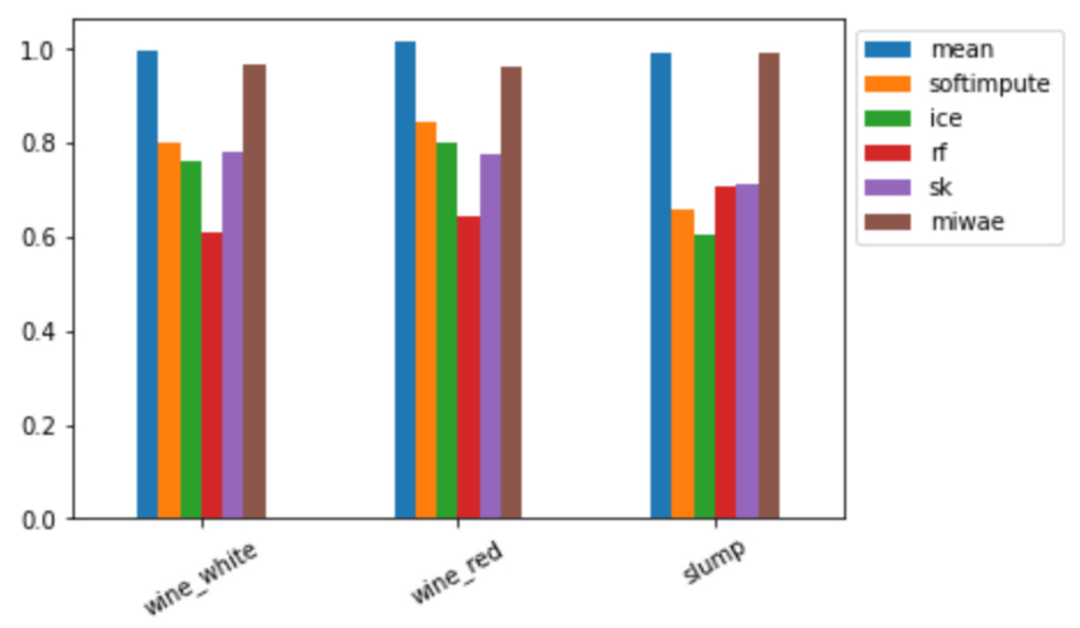
An additional workflow has been written by an external contributor, François Husson (Professor in Statistics, France) and reviewed by us. It specifically compares imputation methods using variational and denoising autoencoders (Gondara and Wang 2018; Mattei and Frellsen 2019; Abiri et al. 2019) with classical methods such as the low-rank based method (Josse et al. 2016). These deep learning methods often require parameter settings. In this workflow, an automatic tuning is suggested. In addition, the methods are compared for several simulation scenarios, when the variables of the dataset are linearly linked or not. In both cases, deep learning methods do not outperform the low-rank method, although they are known to be able to handle non-linear relationships. This workflow is available on our website.

3.3 How to estimate parameters with missing values in R?

This workflow is dedicated to a specific inferential framework when the aim is to estimate linear and logistic regression parameters for multivariate normal data. It is currently only available in R, as there are no analogous implementations available in Python to our knowledge.

In this workflow, two classical methods are compared, using available R implementations: the EM algorithm for logistic and linear regression with the package misaem (Jiang et al. 2020) which uses the SAEM algorithm, Stochastic Approximation of EM algorithm (Delyon et al. 1999) and multiple imputation with the package mice. Both strategies are valid under the MAR missing data mechanism.

The EM algorithm (Dempster et al. 1977) allows to handle MAR missing values in maximum likelihood estimation by integrating over the missing values distribution, conditionally on the observed values. A drawback of this approach is that it requires a separate derivation of the expectation and maximization steps for each model and data type, such as linear regression and logistic regression on multivariate normal covariates. More particularly, multiple imputation allows any method to be applied once the imputation is done, whereas the EM algorithm requires a new variant of the algorithm for each statistical method. Besides, note that mice does not rely on parametric assumptions about the data distribution, whereas misaem assumes Gaussian covariates.

If we assume that we have a binary response variable y and incomplete covariate matrix X_NA composed of five covariates and whose full data counterpart follows a multivariate normal distribution and where the missing values are MAR, we can fit a logistic regression with missing values using the following lines of code.

⬇

1 df_NA <- data.frame(y, X_NA)

2 miss_list <- miss.glm(y~., data=df_NA)

Listing 12: Code to fit a logistic regression model with incomplete covariates using the EM algorithm in R.

This functions miss.glm resembles the standard glm function both in terms of its signature and output. Below we provide an example of output when applying the function summary to the output of the above call to miss.glm.

⬇

1 # Summary

2 print(summary(miss_list))

3 ##

4 ## Call:

5 ## miss.glm(formula = y ~ ., data = df_NA)

6 ##

7 ## Coefficients:

8 ## Estimate Std. Error

9 ## (Intercept) 0.05128 0.31942

10 ## X1 1.05798 0.35989

11 ## X2 -0.99347 0.19620

12 ## X3 1.07606 0.13937

13 ## X4 -0.02258 0.06604

14 ## X5 -1.01527 0.13353

15 ## Log-likelihood: -132.14

Listing 13: Summary of a fitted logistic regression model with incomplete covariates in R.

The rationale behind the popular multiple imputation approach is to create $M>1$ complete datasets by imputing the missing values with “plausible” values, and then to estimate a parameter of interest $\theta$ on each of the imputed datasets. The multiple estimation of $\theta$ and their variability allow to reflect uncertainty due to the unknown missing values. The parameter estimation is performed by applying the analytic method we would have used had the data been complete. We assume that this provides, for each imputed dataset, an estimate of the parameter $\theta$ and an estimate of the corresponding variance. These quantities are finally “pooled” by using specific rules named “Rubin’s rules” (Rubin 2004), leading to a final point estimate with a corresponding estimation of its variance that takes into account the uncertainty due to the missing values. In the following, we will compare this method to EM and illustrate the bias and variance of estimation by an example of simulated dataset.

Using the same example as for the EM algorithm, we can fit a logistic regression model using multiple imputation and inspect its summary as follows:

⬇

1 mi <- mice(data.frame(y, X_NA), m=20) # imputation of 20 complete datasets

2 fit <- with(data = mi, exp = glm(y ~ X1+X2+X3+X4+X5, family = binomial)) # fit

3 beta.mi <- mice::pool(fit) # pool the results using Rubin’s rules

4 summary(beta.mi)

5

6 ## term estimate std.error statistic df p.value

7 ## 1 (Intercept) 0.04006508 0.32034287 0.1250694 325.01965 9.005460e-01

8 ## 2 X1 0.85919319 0.35413092 2.4262021 178.92213 1.625036e-02

9 ## 3 X2 -0.85098985 0.19626265 -4.3359745 123.30329 2.983626e-05

10 ## 4 X3 0.99568077 0.14825886 6.7158263 85.76393 1.934425e-09

11 ## 5 X4 -0.04100766 0.06938153 -0.5910457 126.65685 5.555431e-01

12 ## 6 X5 -0.92834313 0.14636424 -6.3426908 65.36987 2.423562e-08

Listing 14: Code to fit a logistic regression model with incomplete covariates using multiple imputation in R.

For this simulated data set, which follows the multivariate normal distribution, misaem gives less biased results than mice. This was expected as misaem fits here perfectly with the parametric assumptions.

The workflow allows to directly apply and compare these two approaches, using either a simulated dataset, or a custom dataset that the user believes to satisfy the above stated assumptions about the missing data mechanism and distribution of the covariates.

3.4 How to predict in the presence of missing values?

A key task in supervised learning is prediction. Knowing how to predict in the presence of missing values is thus crucial for many practitioners. More precisely, we assume that the missing values occur in the covariates $X$. In this context, the goal is to predict an outcome variable $y$ such that $y=f(X)+\epsilon,$ where $\epsilon$ is a noise term. As a reminder, in supervised learning, the algorithms learn on a training set where the outcome variable is assumed to be known and the results of new (incomplete) observations in the test set are then predicted by applying this learning. Both R and Python workflows present different strategies to deal with the missing values in $X$ (in the train set and in the test set). This task has been studied in detail by Josse et al. 2019. The recommended method is to impute the train set and the test set with the same constant, as the mean, and then apply a universally consistent learner, i.e. very powerful and able to learn any function $f$ (linear or not, etc), such as the gradient boosting. This method has been shown asymptotically consistent. Besides, when random forests are used to impute the missing values, the authors recommend to use the Missing Incorporated in Attributes method (Twala et al. 2008), which allows imputation and prediction to be performed in a single step.

In R

This R workflow has been written by an external contributor of the website, Katarzyna Woźnica (PhD student, Poland). It assesses a popular strategy (two-step strategy) which consists of imputing the train set and the test set independently with the same imputation method and of using usual learning algorithms to predict a target variable. Several imputation methods are compared, such as mice, missForest and softImpute. This work is also available on our website. Note that until recently, using the popular mice package for learning predictive models for incomplete data in R was hindered by the fact that it did not allow to use the same imputation model for the train ad the test set. This has however been addressed and the detail of this recent extension can be found on GitHub.

In Python

The Python workflow proposes to compare two strategies when the aim is to predict a target variable and the covariates may contain missing values:

1. The two-step strategy consists in imputing the missing values both in the train and the test set like mean imputation and IterativeImputer of the scikit-learn library, and to apply usual learning algorithms (such as random forests, gradient boosting, linear regression) on the complete dataset. This learning algorithm can be applied on $X$ but also by adding the response pattern $R$ to the covariates: $[X,R]$.

2. The one-step strategy aims at predicting with learning methods adapted to the missing data without necessarily imputing them, such as the Missing Incorparated in Attributes (MIA) method (Twala et al. 2008).

We propose a function, score_pred, which compares these strategies in terms of prediction performances by introducing missing values in the covariates (x_comp) under a specific missing data mechanism (mecha) and a given percentage of missing values (p). This introduction of missing values is repeated several times (nbsim) which leads to a stochasticity in the results. The dataset is then split into the train set and the test set (75% in the train set, 25% in the test set) and the methods presented below are applied by considering a specific learning algorithm (learner), e.g. the random forests, gradient boosting, linear regression. It returns the prediction error on the test set, by comparing the ground truth (y) and the predicted outcome values on the test set for each simulation (introduction of missing values) in a tabular (see Figure 8) The code of this function is given below, when the learning algorithm is the gradient boosting and 20% of MCAR values are introduced. The covariates $X\in\mathbb{R}^{1000\times 3}$ are generated under the multivariate Gaussian distribution, the parameter of the regression $\beta\in\mathbb{R}^{3}$ is a random uniform distribution. $y$ is generated considering a linear regression such that $y=X\beta+\epsilon,$ with $\epsilon$ a Gaussian noise.

⬇

1 learner = HistGradientBoostingRegressor() #learning algorithm to use

2 p = 0.2

3 res = score_pred(x_comp=X, y = y, learner=learner , p=p,

4 nbsim=10, mecha="MCAR")

Listing 15: Code to compare different strategies to predict an output variable in Python.

Figure 9 shows the graphical output of this function performed for different learning algorithms and for different missing-data mechanisms. When the learner is the linear regression, the two-steps methods with added mask, both for the MCAR mechanism and the MNAR mechanism, performs well. Note that the simulated dataset is generated considering a linear regression, which explains why the linear regression gives better results than other learners. In addition, for the MNAR mechanism, the one-step strategy MIA (especially when the gradient boosting is performed) seems to be a good choice. Note that MIA or mean imputation are recommended asymptotically but when having limited data in the prediction setting, other methods such as multiple imputation can outperform these asymptotically consistent methods (Josse et al. 2019).

Figure 8: Output of the function score_pred to compare different strategies when the aim is to predict in Python. 20% of missing values are introduced in a simulated dataset using the MCAR mechanism. The two-steps strategies (IterativeImputer and the mean imputation) with or without adding a mask and the one-step strategy MIA are compared in terms of prediction error, and then a gradient boosting is performed. The closer the result is to 1, the more accurate the prediction is (1 corresponds to the perfect prediction, 0 to the worst prediction). The results in the tabular corresponds to the prediction error for several simulations (introduction of missing values).

Another function plot_score_realdatasets is specifically designed to handle datasets which already contain missing values. The main arguments are the dataset (X), the outcome variable (y) and the learning algorithm to use (learner) In this case, the stochasticity comes from the way we split the dataset into a train set and a test set. This splitting and subsequent learning is repeated several times.

⬇

1 learner = HistGradientBoostingRegressor() #learning algorithm to

2 p = plot_score_realdatasets(X = X, y = y, learner = learner)

Listing 16: Code to compare different strategies for a real dataset to predict an output variable in Python.

Figure 9: Plot of the function score_pred to compare different strategies when the aim is to predict in Python. 20% of missing values are introduced in a simulated dataset using the MCAR mechanism or the MNAR mechanism. The two-steps strategies (IterativeImputer and the mean imputation) with or without adding a mask and the one-step strategy MIA are compared in terms of prediction error, and several learner are performed (linear regression, random forests, gradient boosting). The closer the result is to 1, the more accurate the prediction is (1 corresponds to the perfect prediction, 0 to the worst prediction).

This concludes the overview over the workflows which have been developed in this project and which we consider as an invitation to other practitioners and researchers to use them for better comparability between methodologies when suggesting new methodologies in research articles and to extend them by providing feedback and ways of improvement which can benefit all potential users.

4 Perspectives and future extensions

By providing a platform and community to discuss missing data, software, approaches and workflows, we are providing a base from which we can grow.

4.1 Towards uniformization and reproducibility

One way to promote and encourage practitioners and researchers in their work with missing values is to provide community benchmarks and workflows centered around missing data. We will continue working on our workflows and the corresponding source code. In doing so we hope to encourage users to continue benchmarking new methods and to present the results in a clear, fair, and reproducible way.

In addition, we plan to propose two types of data challenges - 1) imputation and estimation, and 2) analysis workflows. For the first challenge, the objective is to find the best imputation or estimation strategy. The community would be given a dataset with missing values, for which there is actually a hidden copy of the real values. The community is then tasked with creating imputed values, which are assessed against the original dataset with complete values, to determine which imputation is best. This is similar in spirit to the Netflix prize (Bennett et al. 2007) and the M4 challenge in the time series domain (Makridakis et al. 2018). This benchmarking could be extended to other areas, such as parameter estimation, and predictive modeling with missing data.

Analysis workflow could form another community challenge, assessed in a similar way to existing “datathon” events where entries are assessed by an expert panel. Here the challenge could be to develop workflows and data visualizations from complex data. The data could have challenging features, and be combined from various data with complex structure, such as those data with several types of missingness, images, text, data, longitudinal data, and time series.

As has been demonstrated with data competition, involving the community brings forth many creative solutions and discussions that advance the field, and challenge existing strategies.

4.2 Pedagogical and practical guidance

In addition to the benchmarks and data challenges, we also plan to provide further guidance for both learning or teaching, and for applying the existing methods. For instance, an FAQ section is available on the platform, which answers prominent questions recurrent in lectures and talks, and for which the answers cannot always be found directly in the bibliography and lecture materials. Questions we receive on our platform, via the contact form or at other occasions, will also be posted there together with a concise answer.

4.3 Outreach

Despite the initial anchoring in the R community, we work in close collaboration with other communities, in particular with several developer teams of the scikit-learn library Pedregosa et al. 2011. Such collaborations have allowed us to integrate new workflows, to share respective experiences with missing values and to reach an even larger audience.

4.4 Participation and interaction

This platform is aimed to be for the community, in the sense that we welcome every comment and question, encourage submissions of new work, theoretical or practical, either through the provided contact form or directly via the GitHub project repository. We have already received much useful feedback and contributions from the community, organized several remote calls and working sessions at statistics conferences. We are planning on regularly relaunching calls for new material for the platform, for instance through the R consortium blog, R-bloggers and social media platforms. We also intend to use these channels to communicate more generally about the platform and the topic of missing values.

In order for the platform to be a reference to the community, it needs to provide regularly updated user friendly content. Crucial to this is proposing sustainable and accessible solutions for the maintenance of the R-miss-tastic platform. We hope that the well documented code source of the platform invites contributions and community feedback on this project.

The aim of this platform is to go further than only community participation, namely to seed meaningful community interactions, and make it a hub of communication among groups that rarely exchange, both within, and between academia and industry communities.

4.5 Future extensions

Potential extensions that could be added in future releases of the platform and for which we welcome suggestions and contributions are the following: a workflow with a focus on MNAR data and different solutions that can handle such data (as diversity of existing solutions is large, such a unified workflow will be a consequential contribution); for more applied users, a comparison of computation times of different methods, benchmarked on various types of data; a more and more often encountered problem of missing values in data integration: questions such as what do I do when I have clinical data from multiple centers with different mechanisms of missing values or with systematically missing values in certain data? or what do I do when I have time series and missing values in one of the groups of variables?

More generally, these are a few examples to illustrate how we intend to update the platform with relevant results and recommendations from current research around missing values.

Acknowledgements

This work has partially been funded by the R Consortium, Inc. We would like to thank Steffen Moritz and François Husson for their active support and feedback, all contributors who have generously made their course and tutorial materials available, as well as the contributors to the workflows in R and Python code.

References

- Abiri et al. (2019) Abiri, N., B. Linse, P. Edén, and M. Ohlsson (2019). Establishing strong imputation performance of a denoising autoencoder in a wide range of missing data problems. Neurocomputing 365, 137–146.
- Bennett et al. (2007) Bennett, J., S. Lanning, et al. (2007). The netflix prize. In Proceedings of KDD cup and workshop, Volume 2007, pp. 35. Citeseer.
- Biessmann et al. (2018) Biessmann, F., D. Salinas, S. Schelter, P. Schmidt, and D. Lange (2018). ”deep” learning for missing value imputationin tables with non-numerical data. In Proceedings of the 27th ACM International Conference on Information and Knowledge Management, CIKM ’18, pp. 2017–2025.
- Breiman (2001) Breiman, L. (2001). Random forests. Machine learning 45(1), 5–32.
- Carpenter and Kenward (2012) Carpenter, J. and M. Kenward (2012, December). Multiple Imputation and its Application. John Wiley & Sons.
- Cheng et al. (2015) Cheng, X., D. Cook, and H. Hofmann (2015). Visually exploring missing values in multivariable data using a graphical user interface. Journal of statistical software 68(1), 1–23.
- Delyon et al. (1999) Delyon, B., M. Lavielle, E. Moulines, et al. (1999). Convergence of a stochastic approximation version of the em algorithm. The Annals of Statistics 27(1), 94–128.
- Dempster et al. (1977) Dempster, A. P., N. M. Laird, and D. B. Rubin (1977). Maximum likelihood from incomplete data via the em algorithm. Journal of the Royal Statistical Society: Series B (Methodological) 39(1), 1–22.
- Dua and Graff (2019) Dua, D. and C. Graff (2019). UCI machine learning repository.
- Enders (2010) Enders, C. K. (2010). Applied missing data analysis. Guilford press.
- Gelman and Hill (2011) Gelman, A. and J. Hill (2011). Opening windows to the black box. Journal of Statistical Software 40.
- Gondara and Wang (2018) Gondara, L. and K. Wang (2018). Mida: Multiple imputation using denoising autoencoders. In D. Phung, V. Tseng, G. Webb, B. Ho, M. Ganji, and L. Rashidi (Eds.), Proceedings of the 22nd Pacific-Asia Conference on Knowledge Discovery and Data Mining (PAKDD 2018), Lecture Notes in Computer Science, pp. 260–272. Springer International Publishing.
- Hastie et al. (2015) Hastie, T., R. Mazumder, J. D. Lee, and R. Zadeh (2015). Matrix completion and low-rank svd via fast alternating least squares. The Journal of Machine Learning Research 16(1), 3367–3402.
- Honaker et al. (2011) Honaker, J., G. King, and M. Blackwell (2011). Amelia II: A program for missing data. Journal of Statistical Software 45(7), 1–47.
- Ihaka (1998) Ihaka, R. (1998). R: Past and future history. Computing Science and Statistics 392396.
- Jiang et al. (2020) Jiang, W., J. Josse, M. Lavielle, and T. Group (2020). Logistic regression with missing covariates—parameter estimation, model selection and prediction within a joint-modeling framework. Computational Statistics & Data Analysis 145, 106907.
- Josse et al. (2016) Josse, J., F. Husson, et al. (2016). missmda: a package for handling missing values in multivariate data analysis. Journal of Statistical Software 70(1), 1–31.
- Josse et al. (2019) Josse, J., N. Prost, E. Scornet, and G. Varoquaux (2019). On the consistency of supervised learning with missing values. arXiv preprint.
- Josse and Reiter (2018) Josse, J. and J. P. Reiter (2018). Introduction to the special section on missing data. Statistical Science 33(2), 139–141.
- Kowarik and Templ (2016) Kowarik, A. and M. Templ (2016). Imputation with the R package VIM. Journal of Statistical Software 74(7), 1–16.
- Little and Rubin (2002) Little, R. J. A. and D. B. Rubin (2002, September). Statistical Analysis with Missing Data (2nd ed. ed.). New York ; Chichester: Wiley.
- Makridakis et al. (2018) Makridakis, S., E. Spiliotis, and V. Assimakopoulos (2018). The m4 competition: Results, findings, conclusion and way forward. International Journal of Forecasting 34(4), 802–808.
- Mattei and Frellsen (2019) Mattei, P.-A. and J. Frellsen (2019). Miwae: Deep generative modelling and imputation of incomplete data sets. In International Conference on Machine Learning, pp. 4413–4423. PMLR.
- Mayer et al. (2020) Mayer, I., E. Sverdrup, T. Gauss, J.-D. Moyer, S. Wager, and J. Josse (2020). Doubly robust treatment effect estimation with missing attributes. Ann. Appl. Statist. 14(3), 1409–1431.
- Moritz and Bartz-Beielstein (2017) Moritz, S. and T. Bartz-Beielstein (2017). imputeTS: Time Series Missing Value Imputation in R. The R Journal 9(1), 207–218.
- Murray and Reiter (2015) Murray, J. S. and J. P. Reiter (2015). Multiple imputation of missing categorical and continuous values via bayesian mixture models with local dependence.
- Muzellec et al. (2020) Muzellec, B., J. Josse, C. Boyer, and M. Cuturi (2020). Missing data imputation using optimal transport. In International Conference on Machine Learning, pp. 7130–7140. PMLR.
- Pedregosa et al. (2011) Pedregosa, F., G. Varoquaux, A. Gramfort, V. Michel, B. Thirion, O. Grisel, M. Blondel, P. Prettenhofer, R. Weiss, V. Dubourg, et al. (2011). Scikit-learn: Machine learning in python. the Journal of machine Learning research 12, 2825–2830.
- R Core Team (2020) R Core Team (2020). R: A Language and Environment for Statistical Computing. Vienna, Austria: R Foundation for Statistical Computing.
- Rubin (1976) Rubin, D. B. (1976). Inference and missing data. Biometrika 63(3), 581–592.
- Rubin (2004) Rubin, D. B. (2004). Multiple imputation for nonresponse in surveys, Volume 81. John Wiley & Sons.
- Schafer and Graham (2002) Schafer, J. L. and J. W. Graham (2002, June). Missing data: our view of the state of the art. Psychological methods 7(2), 147–177.
- Seaman et al. (2013) Seaman, S., J. Galati, D. Jackson, and J. Carlin (2013). What is meant by” missing at random”? Statistical Science, 257–268.
- StataCorp. (2019) StataCorp. (2019). Stata Statistical Software: Release 16. College Station, TX: StataCorp LLC.
- Stekhoven and Bühlmann (2012) Stekhoven, D. J. and P. Bühlmann (2012). Missforest—non-parametric missing value imputation for mixed-type data. Bioinformatics 28(1), 112–118.
- Tierney et al. () Tierney, N., D. Cook, M. McBain, and C. Fay. naniar: Data Structures, Summaries, and Visualisations for Missing Data. R package version 0.2.0.
- Tierney and Cook (2018) Tierney, N. J. and D. H. Cook (2018). Expanding tidy data principles to facilitate missing data exploration, visualization and assessment of imputations. arXiv preprint arXiv:1809.02264.
- Twala et al. (2008) Twala, B., M. Jones, and D. J. Hand (2008). Good methods for coping with missing data in decision trees. Pattern Recognition Letters 29(7), 950–956.
- van Buuren (2012) van Buuren, S. (2012, March). Flexible Imputation of Missing Data. CRC Press.
- van Buuren and Groothuis-Oudshoorn (2011) van Buuren, S. and K. Groothuis-Oudshoorn (2011). mice: Multivariate imputation by chained equations in r. Journal of Statistical Software 45(3), 1–67.
- Van Rossum and Drake (2009) Van Rossum, G. and F. L. Drake (2009). Python 3 Reference Manual. Scotts Valley, CA: CreateSpace.
- Xie et al. (2017) Xie, Y., A. Presmanes Hill, and A. Thomas (2017). blogdown: Creating Websites with R Markdow. The R Series. Chapman and Hall/CRC.
- Yoon et al. (2018) Yoon, J., J. Jordon, and M. Schaar (2018). Gain: Missing data imputation using generative adversarial nets. In International Conference on Machine Learning, pp. 5689–5698. PMLR.
- Zhu et al. (2019) Zhu, Z., T. Wang, and R. J. Samworth (2019). High-dimensional principal component analysis with heterogeneous missingness. arXiv preprint arXiv:1906.12125.