arXiv is now an independent nonprofit! Learn more
License: CC BY-NC-ND 4.0
arXiv:1908.04427v6 [stat.ME] 11 Sep 2023

A Groupwise Approach for Inferring Heterogeneous Treatment Effects in Causal Inference

Chan Park    Hyunseung Kang1: Department of Statistics and Data Science, University of Pennsylvania2: Department of Statistics, University of Wisconsin–Madison
Abstract

Recently, there has been great interest in estimating the conditional average treatment effect using flexible machine learning methods. However, in practice, investigators often have working hypotheses about effect heterogeneity across pre-defined subgroups of study units, which we call the groupwise approach. The paper compares two modern ways to estimate groupwise treatment effects, a nonparametric approach and a semiparametric approach, with the goal of better informing practice. Specifically, we compare (a) the underlying assumptions, (b) efficiency and adaption to the underlying data generating models, and (c) a way to combine the two approaches. We also discuss how to test a key assumption concerning the semiparametric estimator and to obtain cluster-robust standard errors if study units in the same subgroups are correlated. We demonstrate our findings by conducting simulation studies and reanalyzing the Early Childhood Longitudinal Study.

Keywords: Conditional average treatment effect, Partially linear model, Semiparametric efficiency, Simultaneous inference

1 Introduction

1.1 Motivation: A Groupwise Approach for Inferring Effect Heterogeneity

Recently, there has been great interest in estimating heterogeneous treatment effects using machine learning methods (Su et al., 2009; Hill, 2011; Athey and Imbens, 2016; Shalit et al., 2017; Chernozhukov et al., 2018; Dorie et al., 2019; Hahn et al., 2020; Kennedy, 2020; Nie and Wager, 2020). A common focus in these works is estimating the conditional average treatment effect (CATE) given a specific value of pp covariates 𝐗ip\mathbf{X}_{i}\in\mathbb{R}^{p}, i.e., τ(𝐗i)=E{Yi(1)Yi(0)|𝐗i}\tau^{*}(\mathbf{X}_{i})={\rm E}\big\{Y_{i}^{(1)}-Y_{i}^{(0)}\,|\,\mathbf{X}_{i}\big\} where Yi(a)Y_{i}^{(a)} is the potential outcome of study unit ii if he/she were to receive a binary treatment value a{0,1}a\in\{0,1\}. However, in practice, investigators often hypothesize and discuss effect heterogeneity based on pre-defined, meaningful subgroups of study units. For example, in our empirical example from McCoy et al. (2016), the authors studied the differential effects of early childhood care on children’s academic achievements among urban and rural communities; see Section 6 for details. We call this approach to studying effect heterogeneity the groupwise approach and the target estimand 𝝉=(τ1,,τG)\bm{\tau}^{*}=(\tau_{1}^{*},\ldots,\tau_{G}^{*})^{\intercal} is formally represented as

τg=E{Yi(1)Yi(0)|M(𝐗i)=g}=E{τ(𝐗i)|M(𝐗i)=g},g=1,,G.\displaystyle\tau_{g}^{*}={\rm E}\big\{Y_{i}^{(1)}-Y_{i}^{(0)}\,|\,M(\mathbf{X}_{i})=g\big\}={\rm E}\big\{\tau^{*}(\mathbf{X}_{i})\,|\,M(\mathbf{X}_{i})=g\big\}\ ,\ g=1,\ldots,G\ . (1)

The function M:𝐗i{1,,G}M:\mathbf{X}_{i}\to\{1,\ldots,G\} is a fixed, well-defined (i.e., Pr{M(𝐗i)=g}\Pr\{M(\mathbf{X}_{i})=g\} is away from 00 and 11) function that partitions the pp-dimensional covariates 𝐗i\mathbf{X}_{i} into GG non-overlapping subgroups and τg\tau_{g}^{*} is the average treatment effect within the ggth subgroup. The main theme of the paper is to carefully examine recent, modern approaches of estimating τg\tau_{g}^{*} based on different models of the observed data and to use the insights from our investigation to better inform practice.

1.2 Nonparametric Versus Semiparametric Approaches to Estimate τg\tau_{g}^{*}

Estimation and inference of τg\tau_{g}^{*} have been discussed in many prior works (Imai and Ratkovic, 2013; Chernozhukov et al., 2017; Künzel et al., 2018; Athey et al., 2019; Kennedy, 2020; Nie and Wager, 2020; Imai and Li, 2022). These works can be roughly divided into two types, a nonparametric approach and a semiparametric approach. A nonparametric approach usually starts by estimating τ(𝐗i)\tau^{*}(\mathbf{X}_{i}) with nonparamteric, machine learning methods, say by the generalized random forest (GRF) (Athey et al., 2019), the XX-learner (Künzel et al., 2019), the RR-learner (Nie and Wager, 2020), or the DRDR-learner (Kennedy, 2020), and averaging τ(𝐗i)\tau^{*}(\mathbf{X}_{i}) over 𝐗i\mathbf{X}_{i} with M(𝐗i)=gM(\mathbf{X}_{i})=g. This approach typically makes no parametric assumptions about the functional form of τ(𝐗i)\tau^{*}(\mathbf{X}_{i}), the outcome regression, or the propensity score (Rosenbaum and Rubin, 1983). In contrast, a semiparametric approach usually makes a semiparametric modeling assumption about τ(𝐗i)\tau^{*}(\mathbf{X}_{i}) where the parametric component of the semiparametric model often equals the target parameter of interest τg\tau_{g}^{*}; see Section 2.2 for details. We remark that there are works that are in-between or outside of the two approaches (Nie and Wager, 2020; Chernozhukov et al., 2017; Imai and Li, 2022). In particular, Chernozhukov et al. (2017) and Imai and Li (2022) focused on estimating a version of the groupwise effects in a randomized experiment with a known propensity score. Specifically, their target estimand is a conditional groupwise effect where the subgroups are random and depend on particular sample-splitting realizations. In contrast, we primarily focus on an observational study with an unknown propensity score. Also, our target estimand, the groupwise effect τg\tau_{g}^{*}, and the subgroups are fixed regardless of sample-splitting realizations.

The paper compares and contrasts the semiparametric approach and the nonparametric approach of estimating τg\tau_{g}^{*}. Some notable results in the paper include (a) a sufficient and necessary condition for the semiparametric estimator to consistently estimate the groupwise effect, (b) efficiency and data-adaptive properties of the estimators from the two approaches, (c) a new, combined estimator that can be more efficient than both estimators, (d) derivation of cluster-robust standard errors of these estimators, and (e) a simple, multiple testing procedure to control for familywise error rate when each component of τg\tau_{g}^{*} are tested simultaneously. For practitioners, we summarize our findings in Figure 3.1.

2 Different Approaches of Estimating Groupwise Effects

2.1 Setup

For each study unit i=1,,Ni=1,\ldots,N, we observe 𝐎i=(Yi,Ai,𝐗i)\mathbf{O}_{i}=(Y_{i},A_{i},\mathbf{X}_{i}) where YiY_{i}\in\mathbb{R} is the outcome, Ai{0,1}A_{i}\in\{0,1\} is the treatment indicator with 1 indicating treatment and 0 indicating control, and 𝐗ip\mathbf{X}_{i}\in\mathbb{R}^{p} are pre-treatment covariates. Let Yi(1)Y_{i}^{(1)} and Yi(0)Y_{i}^{(0)} be the potential outcomes under treatment and control, respectively. Let 𝝉=(τ1,,τG)\bm{\tau}^{*}=(\tau_{1}^{*},\ldots,\tau_{G}^{*})^{\intercal} be the vector of the groupwise treatment effects, which are formally defined in equation (1).

We use the following notations for sets, norms, and convergence. For a subset 𝒮{1,,N}\mathcal{S}\subseteq\{1,\ldots,N\}, we denote its complement 𝒮C={1,,N}𝒮\mathcal{S}^{C}=\{1,\ldots,N\}\setminus\mathcal{S}. We denote both the 2-norm of a vector and the spectral norm of a matrix as 2\|\cdot\|_{2}. For a vector 𝒗\bm{v}, let 𝒗2\bm{v}^{\otimes 2} be the outer product of 𝒗\bm{v}, i.e., 𝒗2=𝒗𝒗\bm{v}^{\otimes 2}=\bm{v}\bm{v}^{\intercal}. Let L2(P)L_{2}(P)-norm for a random variable 𝐖\mathbf{W} and its function h(𝐖)h(\mathbf{W}) be denoted as 𝐖P,r={𝐰2r𝑑P(𝐰)}1/r\|\mathbf{W}\|_{P,r}=\big\{\int\lVert\mathbf{w}\rVert_{2}^{r}\,dP(\mathbf{w})\big\}^{1/r} and hP,r=h(𝐖)P,r={h(𝐰)2r𝑑P(𝐰)}1/r\|h\|_{P,r}=\|h(\mathbf{W})\|_{P,r}=\big\{\int\lVert h(\mathbf{w})\rVert_{2}^{r}\,dP(\mathbf{w})\big\}^{1/r}, respectively, where P(𝐰)P(\mathbf{w}) is the distribution of 𝐖\mathbf{W}. For a sequence aNa_{N}, let 𝐖N=OP(aN)\mathbf{W}_{N}=O_{P}(a_{N}) and 𝐖N=oP(aN)\mathbf{W}_{N}=o_{P}(a_{N}) be the usual big-O and little-O notations, respectively. Let 𝐖ND𝐖\mathbf{W}_{N}\stackrel{{\scriptstyle D}}{{\rightarrow}}\mathbf{W} mean that a random variable 𝐖N\mathbf{W}_{N} converges to 𝐖\mathbf{W} in distribution as NN\rightarrow\infty.

We make the standard causal assumptions for observational data; see Imbens and Rubin (2015) and Hernán and Robins (2020) for textbook discussions.

Assumption 2.1.

Suppose the following conditions hold.

  1. (A1)

    Stable Unit Treatment Value Assumption (SUTVA): Yi=Yi(Ai)Y_{i}=Y_{i}^{(A_{i})} almost surely.

  2. (A2)

    Conditional Ignorability/Unconfoundedness: {Yi(1),Yi(0)}Ai|𝐗i\{Y_{i}^{(1)},Y_{i}^{(0)}\}\rotatebox[origin={c}]{90.0}{$\models$}\,A_{i}\,|\,\mathbf{X}_{i} for all 𝐗i\mathbf{X}_{i}.

  3. (A3)

    Overlap/Positivity: For all 𝐱\mathbf{x} and some positive constant cec_{e}, the propensity score e(𝐱)=Pr(Ai=1|𝐗i=𝐱)e^{*}(\mathbf{x})=\Pr\big(A_{i}=1\,|\,\mathbf{X}_{i}=\mathbf{x}\big) satisfies cee(𝐱)1cec_{e}\leq e^{*}(\mathbf{x})\leq 1-c_{e}.

  4. (A4)

    Well-defined Subgroups: For g=1,,Gg=1,\ldots,G and for some positive constant cMc_{M}, we have cMPr{M(𝐗i)=g}1cMc_{M}\leq\Pr\big\{M(\mathbf{X}_{i})=g\big\}\leq 1-c_{M}.

Under Assumption 2.1, the CATE and the target estimand τg\tau_{g}^{*} are identifiable from the observed data as follows:

τ(𝐱)=μ(1,𝐱)μ(0,𝐱),\displaystyle\tau^{*}(\mathbf{x})=\mu^{*}(1,\mathbf{x})-\mu^{*}(0,\mathbf{x})\ ,
τg={μ(1,𝐱)μ(0,𝐱)}𝟙{M(𝐱)=g}dP𝐗(𝐱)𝟙{M(𝐱)=g}dP𝐗(𝐱),g=1,,G.\displaystyle\tau_{g}^{*}=\frac{\int\{\mu^{*}(1,\mathbf{x})-\mu^{*}(0,\mathbf{x})\}\mathbbm{1}\{M(\mathbf{x})=g\}\,dP_{\mathbf{X}}(\mathbf{x})}{\int\mathbbm{1}\{M(\mathbf{x})=g\}\,dP_{\mathbf{X}}(\mathbf{x})}\ ,\ g=1,\ldots,G\ . (2)

Here, the function μ(Ai,𝐗i)=E(Yi|Ai,𝐗i)\mu^{*}(A_{i},\mathbf{X}_{i})={\rm E}\big(Y_{i}\,|\,A_{i},\mathbf{X}_{i}) is the outcome regression. The rest of the paper discusses the nonparametric and semiparametric approaches of estimating τg\tau_{g}^{*} from equation (2).

2.2 A Semiparametric Estimator τ^SP,g\widehat{\tau}_{{\rm SP},g}

This section reviews a popular, semiparametric approach to estimate τg\tau_{g}^{*} based on the following partially linear outcome model:

Yi\displaystyle Y_{i} =μ(0,𝐗i)+Aig=1Gβg𝟙{M(𝐗i)=g}+ϵi,E(ϵi|Ai,𝐗i)=0,\displaystyle=\mu^{*}(0,\mathbf{X}_{i})+A_{i}\sum_{g=1}^{G}\beta_{g}^{*}\mathbbm{1}\big\{M(\mathbf{X}_{i})=g\big\}+\epsilon_{i}\ ,\ {\rm E}\big(\epsilon_{i}\,|\,A_{i},\mathbf{X}_{i}\big)=0, (PLM)
=μ(0,𝐗i)+Ai𝐈(𝐗i)𝜷+ϵi.\displaystyle=\mu^{*}(0,\mathbf{X}_{i})+A_{i}\mathbf{I}(\mathbf{X}_{i})^{\intercal}\bm{\beta}^{*}+\epsilon_{i}.

Here, 𝐈(𝐗i)=(𝟙{M(𝐗i)=1},,𝟙{M(𝐗i)=G})\mathbf{I}(\mathbf{X}_{i})=\big(\mathbbm{1}\{M(\mathbf{X}_{i})=1\},\ldots,\mathbbm{1}\{M(\mathbf{X}_{i})=G\}\big)^{\intercal} and 𝜷=(β1,,βG)\bm{\beta}^{*}=(\beta_{1}^{*},\ldots,\beta_{G}^{*})^{\intercal}. In words, (PLM) states that study unit ii’s observed outcome shifts by a constant amount βg\beta_{g}^{*} if he/she were treated i.e., Ai=1A_{i}=1, and belonged to group gg. If (PLM) is the correct model for the observed data and the causal identifying assumptions in Assumption 2.1 hold, the causal parameters based on potential outcomes are related to the model parameters based on the observed data as τ(𝐱)=g=1G𝟙{M(𝐱)=g}βg\tau^{*}(\mathbf{x})=\sum_{g=1}^{G}\mathbbm{1}\{M(\mathbf{x})=g\}\beta_{g}^{*} for all 𝐱\mathbf{x} and τg=βg\tau_{g}^{*}=\beta_{g}^{*} for g=1,,Gg=1,\ldots,G.

Robinson (1988) and more recently Chernozhukov et al. (2018) provided a general approach to estimate semiparametric models such as (PLM) by using the following procedure. First, we remove the nonparametric component μ(0,𝐗i)\mu^{*}(0,\mathbf{X}_{i}) in (PLM) by subtracting ν(𝐗i)=E(Yi|𝐗i)\nu^{*}(\mathbf{X}_{i})={\rm E}\big(Y_{i}\,|\,\mathbf{X}_{i}\big) from (PLM). By the definition of conditional expectations, we arrive at

Yiν(𝐗i)={Aie(𝐗i)}𝐈(𝐗i)𝜷+ϵi.\displaystyle Y_{i}-\nu^{*}(\mathbf{X}_{i})=\big\{A_{i}-e^{*}(\mathbf{X}_{i})\big\}\mathbf{I}(\mathbf{X}_{i})^{\intercal}\bm{\beta}^{*}+\epsilon_{i}.

Second, if we define Zi=Yiν(𝐗i)Z_{i}^{*}=Y_{i}-\nu^{*}(\mathbf{X}_{i}) and 𝐕i={Aie(𝐗i)}𝐈(𝐗i)\mathbf{V}_{i}^{*}=\big\{A_{i}-e^{*}(\mathbf{X}_{i})\big\}\mathbf{I}(\mathbf{X}_{i})^{\intercal}, the above model becomes a classic linear regression model with ZiZ_{i}^{*} as a response variable and 𝐕i\mathbf{V}_{i}^{*} as a GG-dimensional regressor. In particular, if the two functions ν\nu^{*} and ee^{*} that define the variables ZiZ_{i}^{*} and 𝐕i\mathbf{V}_{i}^{*} are known, we can use ordinary least squares (OLS) to arrive at consistent and asymptotically normal (CAN) estimators of 𝜷\bm{\beta}^{*}. When ν\nu^{*} and ee^{*} are unknown, we can use cross-fitting (Chernozhukov et al., 2018) where we (i) split the data into two folds, (ii) estimate the two unknown functions ν\nu^{*} and ee^{*} with potentially flexible machine learning methods, (iii) run OLS, and (iv) repeat (i)-(iii); see Algorithm 1 for details.

Original data 𝐎i\mathbf{O}_{i}, i=1,,Ni=1,\ldots,N.
Randomly split data into 1\mathcal{I}_{1}, 2{1,,N}\mathcal{I}_{2}\subseteq\{1,\ldots,N\} where |1|=|2|=N/2|\mathcal{I}_{1}|=|\mathcal{I}_{2}|=N/2 and 12=\mathcal{I}_{1}\cap\mathcal{I}_{2}=\emptyset.
for k=1,2k=1,2 do
  Estimate ν\nu^{*} and ee^{*} with subsample kC\mathcal{I}_{k}^{C}. Denote them as ν^(k)\widehat{\nu}^{(-k)} and e^(k)\widehat{e}^{(-k)}.
  Evaluate ν^(k)(𝐗i)\widehat{\nu}^{(-k)}(\mathbf{X}_{i}) and e^(k)(𝐗i)\widehat{e}^{(-k)}(\mathbf{X}_{i}) for iki\in\mathcal{I}_{k}.
end for
Run OLS by using {Aie^(k)(𝐗i)}𝐈(𝐗i)\{A_{i}-\widehat{e}^{(-k)}(\mathbf{X}_{i})\}\mathbf{I}(\mathbf{X}_{i}) as the regressors and Yiν^(k)(𝐗i)Y_{i}-\widehat{\nu}^{(-k)}(\mathbf{X}_{i}) as the dependent variable.
return A semiparametric estimator of 𝝉\bm{\tau}^{*}, denoted by 𝝉^SP=(τ^SP,1,,τ^SP,G)\widehat{\bm{\tau}}_{{\rm SP}}=(\widehat{\tau}_{{\rm SP},1},\ldots,\widehat{\tau}_{{\rm SP},G})^{\intercal}, and the corresponding variance estimator (σ^SP,12,,σ^SP,G2)(\widehat{\sigma}_{{\rm SP},1}^{2},\ldots,\widehat{\sigma}_{{\rm SP},G}^{2}):
τ^SP,g\displaystyle\widehat{\tau}_{{\rm SP},g} =k=12ik{Yiν^(k)(𝐗i)}{Aie^(k)(𝐗i)}𝟙{M(𝐗i)=g}k=12ik{Aie^(k)(𝐗i)}2𝟙{M(𝐗i)=g},\displaystyle=\frac{\sum_{k=1}^{2}\sum_{i\in\mathcal{I}_{k}}\big\{Y_{i}-\widehat{\nu}^{(-k)}\big(\mathbf{X}_{i}\big)\big\}\big\{A_{i}-\widehat{e}^{(-k)}(\mathbf{X}_{i})\big\}\mathbbm{1}\{M(\mathbf{X}_{i})=g\}}{\sum_{k=1}^{2}\sum_{i\in\mathcal{I}_{k}}\big\{A_{i}-\widehat{e}^{(-k)}(\mathbf{X}_{i})\big\}^{2}\mathbbm{1}\{M(\mathbf{X}_{i})=g\}}\ ,
σ^SP,g2\displaystyle\widehat{\sigma}_{{\rm SP},g}^{2} =1Nk=12ik{ϵ^i(k)}2{Aie^(k)(𝐗i)}2𝟙{M(𝐗i)=g}[1Nk=12ik{Aie^(k)(𝐗i)}2𝟙{M(𝐗i)=g}]2,\displaystyle=\frac{\frac{1}{N}\sum_{k=1}^{2}\sum_{i\in\mathcal{I}_{k}}\{\widehat{\epsilon}_{i}^{(-k)}\}^{2}\big\{A_{i}-\widehat{e}^{(-k)}(\mathbf{X}_{i})\big\}^{2}\mathbbm{1}\big\{M(\mathbf{X}_{i})=g\big\}}{\big[\frac{1}{N}\sum_{k=1}^{2}\sum_{i\in\mathcal{I}_{k}}\big\{A_{i}-\widehat{e}^{(-k)}(\mathbf{X}_{i})\big\}^{2}\mathbbm{1}\big\{M(\mathbf{X}_{i})=g\big\}\big]^{2}}\ ,\ (3)
ϵ^i(k)\displaystyle\widehat{\epsilon}_{i}^{(-k)} ={Yiν^(k)(𝐗i)}{Aie^(k)(𝐗i)}𝐈(𝐗i)𝝉^SP.\displaystyle=\big\{Y_{i}-\widehat{\nu}^{(-k)}\big(\mathbf{X}_{i}\big)\big\}-\big\{A_{i}-\widehat{e}^{(-k)}(\mathbf{X}_{i})\big\}\mathbf{I}(\mathbf{X}_{i})^{\intercal}\widehat{\bm{\tau}}_{\rm SP}\ .
Algorithm 1 A Semiparametric Estimator for Groupwise Treatment Effects

We make some brief remarks about the semiparametric estimator 𝝉^SP\widehat{\bm{\tau}}_{{\rm SP}}. First, 𝝉^SP\widehat{\bm{\tau}}_{{\rm SP}} is a special case of the RR-learner (Nie and Wager, 2020) where the RR-learner estimates the entire CATE function τ(𝐗i)\tau^{*}(\mathbf{X}_{i}) across all 𝐗i\mathbf{X}_{i} in a data-adaptive manner without specifying subgroups. In contrast, our task is to provide a group-level summary of the CATE function where the subgroups are specified a priori by investigators. Second, under (PLM), τ(𝐗i)\tau^{*}(\mathbf{X}_{i}) in equation (4) of Nie and Wager (2020) is represented by GG finite-dimensional parameters. Third, we can split the sample into more than two folds to stabilize the cross-fitted estimators.

2.3 A Nonparametric Estimator τ^NP,g\widehat{\tau}_{{\rm NP},g}

This section reviews a popular, nonparametric approach to estimate groupwise effects based on the following, nonparametric linear model of the outcome:

Yi=μ(0,𝐗i)+Aiγ(𝐗i)+ϵi,E(ϵi|Ai,𝐗i)=0.Y_{i}=\mu^{*}(0,\mathbf{X}_{i})+A_{i}\gamma^{*}(\mathbf{X}_{i})+\epsilon_{i},\ {\rm E}(\epsilon_{i}\,|\,A_{i},\mathbf{X}_{i})=0. (NPM)

Here, γ\gamma^{*} is a nonparametric function. In words, (NPM) states that study unit ii’s observed outcome shifts by an amount γ(𝐗i)\gamma^{*}(\mathbf{X}_{i}) if study unit ii is treated. Compared to (PLM), two people in the same subgroup gg may have their outcomes shifted by a different amount depending on their respective covariates. Also, unlike (PLM), (NPM) does not make any parametric or semiparametric assumptions about the outcome; the outcome is determined by two nonparametric functions μ\mu^{*} and γ\gamma^{*}. Finally, if the causal identifying assumptions in Assumption 2.1 hold, the causal parameters based on potential outcomes are related to the model parameters based on the observed data as follows: τ(𝐱)=γ(𝐱)\tau^{*}(\mathbf{x})=\gamma^{*}(\mathbf{x}) and τg=E{γ(𝐗i)|M(𝐗i)=g}\tau_{g}^{*}={\rm E}\{\gamma^{*}(\mathbf{X}_{i})\,|\,M(\mathbf{X}_{i})=g\} for g=1,,Gg=1,\ldots,G.

We can adapt the results in Robins (1994), Hahn (1998), Scharfstein et al. (1999), and van der Laan and Robins (2003) to obtain an estimator of τg\tau_{g}^{*} under (NPM). Specifically, our nonparametric estimator is based on the efficient influence function for the average treatment effect, denoted by φ(𝐎i)\varphi^{*}(\mathbf{O}_{i}), which is formally stated below:

φ(𝐎i)={Aie(𝐗i)1Ai1e(𝐗i)}{Yiμ(Ai,𝐗i)}+μ(1,𝐗i)μ(0,𝐗i).\displaystyle\varphi^{*}(\mathbf{O}_{i})=\bigg\{\frac{A_{i}}{e^{*}(\mathbf{X}_{i})}-\frac{1-A_{i}}{1-e^{*}(\mathbf{X}_{i})}\bigg\}\{Y_{i}-\mu^{*}(A_{i},\mathbf{X}_{i})\}+\mu^{*}(1,\mathbf{X}_{i})-\mu^{*}(0,\mathbf{X}_{i})\ .

To estimate groupwise effects, we can run a linear regression with φ(𝐎i)\varphi^{*}(\mathbf{O}_{i}) as a response variable and the dummy variables representing each group gg (without the intercept term) as regressors. Also, we can use plug-in estimators from cross-fitting, similar to the semiparametric approach, to estimate the two unknown functions μ\mu^{*} and ee^{*} in φ(𝐎i)\varphi^{*}(\mathbf{O}_{i}); see Algorithm 2 for details.

Original data 𝐎i\mathbf{O}_{i}, i=1,,Ni=1,\ldots,N.
Randomly split data into 1\mathcal{I}_{1}, 2{1,,N}\mathcal{I}_{2}\subseteq\{1,\ldots,N\} where |1|=|2|=N/2|\mathcal{I}_{1}|=|\mathcal{I}_{2}|=N/2 and 12=\mathcal{I}_{1}\cap\mathcal{I}_{2}=\emptyset.
for k=1,2k=1,2 do
  Estimate μ(1,𝐗i),μ(0,𝐗i)\mu^{*}(1,\mathbf{X}_{i}),\mu^{*}(0,\mathbf{X}_{i}), and e(𝐗i)e^{*}(\mathbf{X}_{i}) with subsample kC\mathcal{I}_{k}^{C}.
  Denote them as μ^(k)(1,𝐗i),μ^(k)(0,𝐗i)\widehat{\mu}^{(-k)}(1,\mathbf{X}_{i}),\widehat{\mu}^{(-k)}(0,\mathbf{X}_{i}), and e^(k)(𝐗i)\widehat{e}^{(-k)}(\mathbf{X}_{i}).
  Evaluate the efficient influence function using the estimated nuisance functions for iki\in\mathcal{I}_{k}, i.e.,
φ^(k)(𝐎i)={Aie^(k)(𝐗i)1Ai1e^(k)(𝐗i)}{Yiμ^(k)(Ai,𝐗i)}\displaystyle\widehat{\varphi}^{(-k)}(\mathbf{O}_{i})=\bigg\{\frac{A_{i}}{\widehat{e}^{(-k)}(\mathbf{X}_{i})}-\frac{1-A_{i}}{1-\widehat{e}^{(-k)}(\mathbf{X}_{i})}\bigg\}\{Y_{i}-\widehat{\mu}^{(-k)}(A_{i},\mathbf{X}_{i})\}
+μ^(k)(1,𝐗i)μ^(k)(0,𝐗i)\displaystyle\hskip 56.9055pt+\widehat{\mu}^{(-k)}(1,\mathbf{X}_{i})-\widehat{\mu}^{(-k)}(0,\mathbf{X}_{i})
end for
Run OLS by using 𝐈(𝐗i)\mathbf{I}(\mathbf{X}_{i}) as the regressors and φ^(k)(𝐎i)\widehat{\varphi}^{(-k)}(\mathbf{O}_{i}) as the dependent variable.
return A nonparametric estimator of 𝝉\bm{\tau}^{*}, denoted by 𝝉^NP=(τ^NP,1,,τ^NP,G)\widehat{\bm{\tau}}_{{\rm NP}}=(\widehat{\tau}_{{\rm NP},1},\ldots,\widehat{\tau}_{{\rm NP},G})^{\intercal}, and the corresponding variance estimator (σ^NP,12,,σ^NP,G2)(\widehat{\sigma}_{{\rm NP},1}^{2},\ldots,\widehat{\sigma}_{{\rm NP},G}^{2}):
τ^NP,g=k=12ikφ^(k)(𝐎i)𝟙{M(𝐗i)=g}i=1N𝟙{M(𝐗i)=g},\displaystyle\widehat{\tau}_{{\rm NP},g}=\frac{\sum_{k=1}^{2}\sum_{i\in\mathcal{I}_{k}}\widehat{\varphi}^{(-k)}(\mathbf{O}_{i})\mathbbm{1}\big\{M(\mathbf{X}_{i})=g\big\}}{\sum_{i=1}^{N}\mathbbm{1}\big\{M(\mathbf{X}_{i})=g\big\}}\ ,
σ^NP,g2=1Nk=12ik{φ^(k)(𝐎i)𝐈(𝐗i)𝝉^NP}2𝟙{M(𝐗i)=g}[1Ni=1N𝟙{M(𝐗i)=g}]2.\displaystyle\widehat{\sigma}_{{\rm NP},g}^{2}=\frac{\frac{1}{N}\sum_{k=1}^{2}\sum_{i\in\mathcal{I}_{k}}\big\{\widehat{\varphi}^{(-k)}(\mathbf{O}_{i})-\mathbf{I}(\mathbf{X}_{i})^{\intercal}\widehat{\bm{\tau}}_{\rm NP}\big\}^{2}\mathbbm{1}\{M(\mathbf{X}_{i})=g\}}{\big[\frac{1}{N}\sum_{i=1}^{N}\mathbbm{1}\{M(\mathbf{X}_{i})=g\}\big]^{2}}\ . (4)
Algorithm 2 A Nonparametric Approach for Groupwise Treatment Effects

2.4 A Combined Estimator τ^W,g\widehat{\tau}_{{\rm W},g}

Suppose an investigator wants to combine the estimators from the semiparametric approach and the nonparametric approach. While the motivation for such an estimator may seem odd at first, especially since the nonparametric approach makes fewer assumptions than the semiparametric approach in terms of modeling assumptions, we show in Section 3.4 how this combined estimator can achieve better performance than either estimator alone in some settings. Formally, for each group gg, consider the weighted combination of the nonparametric and the semiparametric estimators where the weight is the value that minimizes the estimated variance of the combined estimator τ^W,g\widehat{\tau}_{{\rm W},g}, i.e.,

τ^W,g=w^gτ^SP,g+(1w^g)τ^NP,g,\displaystyle\widehat{\tau}_{{\rm W},g}=\widehat{w}_{g}\widehat{\tau}_{{\rm SP},g}+(1-\widehat{w}_{g})\widehat{\tau}_{{\rm NP},g}\ , (5)
w^g=argminw[0,1]Var^{wτ^SP,g+(1w)τ^NP,g}=(σ^NP,g2σ^SP,NP,gσ^SP,g22σ^SP,NP,g+σ^NP,g2)[0,1].\displaystyle\widehat{w}_{g}=\argmin_{w\in[0,1]}\widehat{{\rm Var}}\Big\{w\widehat{\tau}_{{\rm SP},g}+(1-w)\widehat{\tau}_{{\rm NP},g}\Big\}=\bigg(\frac{\widehat{\sigma}_{{\rm NP},g}^{2}-\widehat{\sigma}_{{\rm SP},{\rm NP},g}}{\widehat{\sigma}_{{\rm SP},g}^{2}-2\widehat{\sigma}_{{\rm SP},{\rm NP},g}+\widehat{\sigma}_{{\rm NP},g}^{2}}\bigg)_{[0,1]}\ .

Here, the function (t)[0,1]=t𝟙(0<t<1)+𝟙(t1)(t)_{[0,1]}=t\mathbbm{1}(0<t<1)+\mathbbm{1}(t\geq 1) winsorizes tt\in\mathbb{R} to be between 00 and 11. The term σ^SP,NP,g\widehat{\sigma}_{{\rm SP},{\rm NP},g} is the estimator of the covariance between τ^SP,g\widehat{\tau}_{{\rm SP},g} and τ^NP,g\widehat{\tau}_{{\rm NP},g} and has the form

σ^SP,NP,g\displaystyle\widehat{\sigma}_{{\rm SP},{\rm NP},g} (6)
=1Nk=12ikϵ^i(k){Aie^(k)(𝐗i)}{φ^(k)(𝐎i)𝐈(𝐗i)𝝉^NP}𝟙{M(𝐗i)=g}[1Ni=1N𝟙{M(𝐗i)=g}][1Nk=12ik{Aie^(k)(𝐗i)}2𝟙{M(𝐗i)=g}].\displaystyle=\frac{\frac{1}{N}\sum_{k=1}^{2}\sum_{i\in\mathcal{I}_{k}}\widehat{\epsilon}_{i}^{(-k)}\big\{A_{i}-\widehat{e}^{(-k)}(\mathbf{X}_{i})\big\}\big\{\widehat{\varphi}^{(-k)}(\mathbf{O}_{i})-\mathbf{I}(\mathbf{X}_{i})^{\intercal}\widehat{\bm{\tau}}_{\rm NP}\big\}\mathbbm{1}\{M(\mathbf{X}_{i})=g\}}{\big[\frac{1}{N}\sum_{i=1}^{N}\mathbbm{1}\{M(\mathbf{X}_{i})=g\}\big]\big[\frac{1}{N}\sum_{k=1}^{2}\sum_{i\in\mathcal{I}_{k}}\big\{A_{i}-\widehat{e}^{(-k)}(\mathbf{X}_{i})\big\}^{2}\mathbbm{1}\big\{M(\mathbf{X}_{i})=g\big\}\big]}\ .

By construction, the estimated variance of τ^W,g\widehat{\tau}_{{\rm W},g} is always less than or equal to those of τ^SP,g\widehat{\tau}_{{\rm SP},g} and τ^NP,g\widehat{\tau}_{{\rm NP},g}. Also, from simple algebra, τ^W,g\widehat{\tau}_{{\rm W},g} collapses to τ^SP\widehat{\tau}_{{\rm SP}} if ρ^gσ^SP,g/σ^NP,g\widehat{\rho}_{g}\geq\widehat{\sigma}_{{\rm SP},g}/\widehat{\sigma}_{{\rm NP},g} where ρ^g\widehat{\rho}_{g} is the estimator of the correlation coefficient of the two estimators, i.e., ρ^g=σ^SP,NP,g/(σ^SP,gσ^NP,g)\widehat{\rho}_{g}=\widehat{\sigma}_{{\rm SP},{\rm NP},g}/\big(\widehat{\sigma}_{{\rm SP},g}\widehat{\sigma}_{{\rm NP},g}). Similarly, τ^W,g\widehat{\tau}_{{\rm W},g} collapses to τ^NP\widehat{\tau}_{{\rm NP}} if ρ^gσ^NP,g/σ^SP,g\widehat{\rho}_{g}\geq\widehat{\sigma}_{{\rm NP},g}/\widehat{\sigma}_{{\rm SP},g}. Finally, we remark that τ^W,g\widehat{\tau}_{{\rm W},g} is a special case of some existing estimators that combine two estimators with respect to the squared error loss and one of the two estimators is potentially biased while the other estimator is unbiased (Green and Strawderman, 1991; Green et al., 2005; Mittelhammer and Judge, 2005; Rosenman and Miratrix, 2022).

3 Statistical Properties of Estimators

3.1 Nonparametric and Semiparametric Models

To characterize the properties of the estimators discussed above, we first define the nonparametric model NP\mathcal{M}_{{\rm NP}} and the semiparametric model SP\mathcal{M}_{{\rm SP}}:

NP={P|P is a regular law (Bickel et al., 1998, Chapter 3)},\displaystyle\mathcal{M}_{{\rm NP}}=\big\{P\,\big|\,\text{$P$ is a regular law \cite[citep]{(\@@bibref{AuthorsPhrase1Year}{BKRW1998}{\@@citephrase{, }}{}, Chapter 3)}}\big\}\ ,
SP={PNP|P satisfies (SP) below},\displaystyle\mathcal{M}_{{\rm SP}}=\big\{P\in\mathcal{M}_{\rm NP}\,|\,P\text{ satisfies }\eqref{eq:modelsp}\text{ below}\big\}\ ,
E[{Aie(𝐗i)}2{τ(𝐗i)τg}|M(𝐗i)=g]=0,g=1,,G.\displaystyle{\rm E}\big[\{A_{i}-e^{*}(\mathbf{X}_{i})\}^{2}\{\tau^{*}(\mathbf{X}_{i})-\tau_{g}^{*}\}\,|\,M(\mathbf{X}_{i})=g\big]=0\ ,\ g=1,\ldots,G\ . (SP)

The nonparametric model NP\mathcal{M}_{{\rm NP}} does not restrict the distribution of the observed data whereas the semiparametric model SP\mathcal{M}_{{\rm SP}} restricts the observed data with the moment condition (SP). While (SP) may seem obscure at first, in the next section, we show that (SP) is a necessary and sufficient condition for the semiparametric estimator 𝝉^SP\widehat{\bm{\tau}}_{{\rm SP}} to be CAN for the 𝝉\bm{\tau}^{*}. Also, in Section 4.1, we present a falsification test for (SP) with the observed data. Finally, there are two familiar sufficient (but not necessary) conditions for (SP), which are defined as the following two models PLM.Hom\mathcal{M}_{{{\rm PLM.Hom}}} and Str.Exp\mathcal{M}_{{{\rm Str.Exp}}}:

PLM.Hom={PNP|1.(PLM) holds; and 2.E(ϵi2|Ai,𝐗i)=σg2 for any (Ai,𝐗i)satisfying M(𝐗i)=g{1,,G}.},\displaystyle\mathcal{M}_{{{\rm PLM.Hom}}}=\left\{P\in\mathcal{M}_{\rm NP}\,\left|\begin{array}[]{ll}1.&\hskip-5.69046pt\eqref{model-PLM}\text{ holds; and }\\ 2.&\hskip-5.69046pt\text{${\rm E}(\epsilon_{i}^{2}\,|\,A_{i},\mathbf{X}_{i})=\sigma_{g}^{2}$ for any $(A_{i},\mathbf{X}_{i})$}\\ &\hskip-5.69046pt\text{satisfying $M(\mathbf{X}_{i})=g\in\{1,\ldots,G\}$}.\end{array}\right.\right\},
Str.Exp={PNP|e(𝐗i)=eg for any 𝐗isatisfying M(𝐗i)=g{1,,G}}.\displaystyle\mathcal{M}_{{{\rm Str.Exp}}}=\left\{P\in\mathcal{M}_{\rm NP}\,\left|\begin{array}[]{ll}e^{*}(\mathbf{X}_{i})=e_{g}^{*}\text{ for any }\mathbf{X}_{i}\\ \text{satisfying }M(\mathbf{X}_{i})=g\in\{1,\ldots,G\}\end{array}\right.\right\}.

In words, PLM.Hom\mathcal{M}_{{{\rm PLM.Hom}}} consists of all homoskedastic partially linear outcome models in (PLM). In fact, regardless of whether the error is homoskedastic, all partially linear outcome models in (PLM) satisfy (SP) and thus, all partially linear outcome models are nested in the semiparametric model SP\mathcal{M}_{{\rm SP}}. However, due to its unique theoretical properties, we focus on homoskedastic partial linear models; see Sections 3.2-3.4 for details. The other model Str.Exp\mathcal{M}_{{{\rm Str.Exp}}} consists of data from a stratified randomized experiment where study units in group gg are randomly assigned to treatment with probability ege_{g}^{*}. From straightforward algebra, one can show that any distribution in Str.Exp\mathcal{M}_{{{\rm Str.Exp}}} automatically satisfies condition (SP) by the experimental design, implying that Str.Exp\mathcal{M}_{{{\rm Str.Exp}}} is nested in SP\mathcal{M}_{{\rm SP}}. Therefore, we have the relationships PLM.Hom{PNP|P satisfies (PLM)}SPNP\mathcal{M}_{{{\rm PLM.Hom}}}\subset\{P\in\mathcal{M}_{\rm NP}\,|\,\text{$P$ satisfies \eqref{model-PLM}}\}\subset\mathcal{M}_{{\rm SP}}\subset\mathcal{M}_{{\rm NP}} and Str.ExpSPNP\mathcal{M}_{{{\rm Str.Exp}}}\subset\mathcal{M}_{{\rm SP}}\subset\mathcal{M}_{{\rm NP}}, and all of these inclusions are strict.

We conclude by making the following moment assumptions which we use throughout the paper.

Assumption 3.1.

There exist constants CϵC_{\epsilon} and CμC_{\mu} so that the variance of the error E(ϵi2|Ai,𝐗i){\rm E}(\epsilon_{i}^{2}\,|\,A_{i},\mathbf{X}_{i}) and the outcome regression μ(Ai,𝐗i)\mu^{*}(A_{i},\mathbf{X}_{i}) satisfy E(ϵi2|Ai,𝐗i)Cϵ{\rm E}(\epsilon_{i}^{2}\,|\,A_{i},\mathbf{X}_{i})\leq C_{\epsilon} and μ(Ai,𝐗i)[Cμ,Cμ]\mu^{*}(A_{i},\mathbf{X}_{i})\in[-C_{\mu},C_{\mu}] for all (Ai,𝐗i)(A_{i},\mathbf{X}_{i}).

Assumption 3.1 implies that the outcome has a finite variance given (Ai,𝐗i)(A_{i},\mathbf{X}_{i}), and the assumption will automatically hold if the outcome is uniformly bounded.

3.2 Properties of the Semiparametric Estimator

We first characterize properties of the semiparametric estimator 𝝉^SP\widehat{\bm{\tau}}_{{\rm SP}}. We make the following assumption to make progress:

Assumption 3.2.

The nuisance functions used in Algorithm 1 satisfy the following conditions for k=1,2k=1,2:

  1. (a)

    Bounded Nuisance Functions: There exist constants Cν^C_{\widehat{\nu}} and Ce^C_{\widehat{e}} so that ν^(k)(𝐗i)\widehat{\nu}^{(-k)}\big(\mathbf{X}_{i}\big) and e^(k)(𝐗i)\widehat{e}^{(-k)}\big(\mathbf{X}_{i}\big) satisfy ν^(k)(𝐗i)[Cν^,Cν^]\widehat{\nu}^{(-k)}\big(\mathbf{X}_{i}\big)\in[-C_{\widehat{\nu}},C_{\widehat{\nu}}] and e^(k)(𝐗i)[Ce^,1Ce^]\widehat{e}^{(-k)}\big(\mathbf{X}_{i}\big)\in[C_{\widehat{e}},1-C_{\widehat{e}}] for all 𝐗i\mathbf{X}_{i}.

  2. (b)

    Consistency of ν^(k)\widehat{\nu}^{(-k)} and e^(k)\widehat{e}^{(-k)}: ν^(k)(𝐗i)ν(𝐗i)P,2=OP(rν,N)\big\|\widehat{\nu}^{(-k)}(\mathbf{X}_{i})-\nu^{*}(\mathbf{X}_{i})\big\|_{P,2}=O_{P}(r_{\nu,N}) and e^(k)(𝐗i)e(𝐗i)P,2=OP(re,N)\big\|\widehat{e}^{(-k)}(\mathbf{X}_{i})-e^{*}(\mathbf{X}_{i})\big\|_{P,2}=O_{P}(r_{e,N}) where rν,N=o(1)r_{\nu,N}=o(1), re,N=o(N1/4)r_{e,N}=o(N^{-1/4}) and rν,Nre,N=o(N1/2)r_{\nu,N}r_{e,N}=o(N^{-1/2}) as NN\to\infty.

Condition (a) in Assumption 3.2 is a bounded moment condition and this condition is satisfied if the outcome is uniformly bounded. Condition (b) controls how fast the estimated functions converge and this condition can be satisfied by many data-adaptive supervised learning methods such as the Nadaraya–Watson kernel regression estimator (Nadaraya, 1964; Watson, 1964), penalized generalized linear models (Bickel et al., 2009), random forests (Wager and Walther, 2016), and the highly-adaptive lasso (Benkeser and van der Laan, 2016) under mild conditions. Also, condition (b) matches Assumption 4.1 of Chernozhukov et al. (2018), which is used to prove the asymptotic normality of partialling-out/“Robinson-style” estimators (Robinson, 1988). Finally, our condition (b) is weaker than conditions in Lemma 2 of Nie and Wager (2020) since our target estimand (i.e., a GG-dimensional parameter) is statistically simpler than Nie and Wager (2020)’s target estimand (i.e., a function).

Theorem 3.1 describes the asymptotic properties of 𝝉^SP\widehat{\bm{\tau}}_{{\rm SP}} under the semiparametric model SP\mathcal{M}_{{\rm SP}}.

Theorem 3.1.

Suppose that Assumptions 2.1, 3.1 and 3.2 hold. If the observed data PP belongs to SP\mathcal{M}_{{\rm SP}}, the following results hold:

  • (a) The estimator 𝝉^SP\widehat{\bm{\tau}}_{{\rm SP}} is CAN for the groupwise effect 𝝉\bm{\tau}^{*} with a diagonal covariance ΣSP=diag(σSP,12,,σSP,G2)\Sigma_{\rm SP}={\rm diag}(\sigma_{{\rm SP},1}^{2},\ldots,\sigma_{{\rm SP},G}^{2}):

    N(𝝉^SP𝝉)DN(0,ΣSP),σSP,g2=E[ϵi2{Aie(𝐗i)}2𝟙{M(𝐗i)=g}][E[{Aie(𝐗i)}2𝟙{M(𝐗i)=g}]]2.\displaystyle\sqrt{N}\Big(\widehat{\bm{\tau}}_{{\rm SP}}-\bm{\tau}^{*}\Big)\stackrel{{\scriptstyle D}}{{\rightarrow}}N\Big(0,\Sigma_{\rm SP}\Big)\ ,\ \sigma_{{\rm SP},g}^{2}=\frac{{\rm E}\big[\epsilon_{i}^{2}\big\{A_{i}-e^{*}(\mathbf{X}_{i})\big\}^{2}\mathbbm{1}\{M(\mathbf{X}_{i})=g\}\big]}{\big[{\rm E}\big[\big\{A_{i}-e^{*}(\mathbf{X}_{i})\big\}^{2}\mathbbm{1}\{M(\mathbf{X}_{i})=g\}\big]\big]^{2}}\ .

    Also, ΣSP\Sigma_{{\rm SP}} can be consistently estimated by the following plug-in estimator Σ^SP=diag(σ^SP,12,,σ^SP,G2)\widehat{\Sigma}_{{\rm SP}}={\rm diag}(\widehat{\sigma}_{{\rm SP},1}^{2},\ldots,\widehat{\sigma}_{{\rm SP},G}^{2}) where σ^SP,g2\widehat{\sigma}_{{\rm SP},g}^{2} is given in Algorithm 1.

  • (b) The semiparametric estimator 𝝉^SP\widehat{\bm{\tau}}_{{\rm SP}} is locally efficient for 𝝉\bm{\tau}^{*} in the sense that the variance ΣSP\Sigma_{{\rm SP}} is equal to the the semiparametric efficiency bound under model SP\mathcal{M}_{{\rm SP}} at model PLM.Hom\mathcal{M}_{{{\rm PLM.Hom}}}.

Part (a) of Theorem 3.1 states that the semiparametric estimator 𝝉^SP\widehat{\bm{\tau}}_{{\rm SP}} is CAN for 𝝉\bm{\tau}^{*} under the semiparametric model SP\mathcal{M}_{{\rm SP}}, and the asymptotic variance can be consistently estimated. Part (b) of Theorem 3.1 states that 𝝉^SP\widehat{\bm{\tau}}_{{\rm SP}} is locally efficient when the outcome follows a homoskedastic partially linear outcome model in PLM.Hom\mathcal{M}_{{{\rm PLM.Hom}}}. In this case, σSP,g2\sigma_{{\rm SP},g}^{2} reduces to σSP,g2=σg2/E[{Aie(𝐗i)}2𝟙{M(𝐗i)=g}]\sigma_{{\rm SP},g}^{2}=\sigma_{g}^{2}/{\rm E}\big[\big\{A_{i}-e^{*}(\mathbf{X}_{i})\big\}^{2}\mathbbm{1}\{M(\mathbf{X}_{i})=g\}\big], where σg2\sigma_{g}^{2} is the variance of the error associated with the ggth subgroup; see (3.1). Also, σSP,g2\sigma_{{\rm SP},g}^{2} coincides with the semiparametric efficiency bound for τg\tau_{g}^{*} under model PLM.Hom\mathcal{M}_{{{\rm PLM.Hom}}} (Robinson, 1988; Chamberlain, 1992). Critically, 𝝉^SP\widehat{\bm{\tau}}_{{\rm SP}} is not efficient in the larger model SP\mathcal{M}_{{\rm SP}}, say a heteroskedastic partially linear outcome model. This phenomenon is similar to the OLS estimator being efficient under a homoskedastic linear model, but being inefficient under a larger, linear model that includes homokedastic or heteroskedastic variance; see Section 3.4 for additional discussions.

Theorem 3.2 shows that if the semiparametric model SP\mathcal{M}_{{\rm SP}} in Theorem 3.1 does not holds, the semiparametric estimator 𝝉^SP\widehat{\bm{\tau}}_{{\rm SP}} is no longer CAN for 𝝉\bm{\tau}^{*}.

Theorem 3.2.

Suppose that Assumptions 2.1, 3.1, and 3.2 hold. If PP does not belong to SP\mathcal{M}_{{\rm SP}}, i.e., PNPSPCP\in\mathcal{M}_{{\rm NP}}\cap\mathcal{M}_{{\rm SP}}^{C}, the estimator 𝛕^SP\widehat{\bm{\tau}}_{{\rm SP}} is CAN for the overlap-weighted groupwise treatment effect 𝛕OV=(τOV,1,,τOV,G)\bm{\tau}_{{\rm OV}}^{*}=(\tau_{{\rm OV},1}^{*},\ldots,\tau_{{\rm OV},G}^{*})^{\intercal} (Crump et al., 2006; Crump et al., 2009):

N(𝝉^SP𝝉OV)DN(0,ΣSP),τOV,g=E[e(𝐗i){1e(𝐗i)}τ(𝐗i)|M(𝐗i)=g]E[e(𝐗i){1e(𝐗i)}|M(𝐗i)=g].\displaystyle\sqrt{N}(\widehat{\bm{\tau}}_{{\rm SP}}-\bm{\tau}_{{\rm OV}}^{*})\stackrel{{\scriptstyle D}}{{\rightarrow}}N(0,\Sigma_{{\rm SP}}),\ \tau_{{\rm OV},g}^{*}=\frac{{\rm E}\big[e^{*}(\mathbf{X}_{i})\{1-e^{*}(\mathbf{X}_{i})\}\tau^{*}(\mathbf{X}_{i})\,|\,M(\mathbf{X}_{i})=g\big]}{{\rm E}\big[e^{*}(\mathbf{X}_{i})\{1-e^{*}(\mathbf{X}_{i})\}\,|\,M(\mathbf{X}_{i})=g\big]}\ .

Also, the variance ΣSP\Sigma_{{\rm SP}} and its consistent estimator Σ^SP\widehat{\Sigma}_{{\rm SP}} have the same form as Theorem 3.1.

Theorem 3.2 states that, outside of the semiparametric model SP\mathcal{M}_{{\rm SP}}, the semiparametric estimator 𝝉^SP\widehat{\bm{\tau}}_{{\rm SP}} is still asymptotically normal, but converges to a version of the overlap-weighted treatment effect in Crump et al. (2006); Crump et al. (2009) stratified by subgroups. Also, by combining Theorems 3.1 and 3.2, we obtain the following necessary and sufficient condition for 𝝉^SP\widehat{\bm{\tau}}_{{\rm SP}} to be CAN for the original target estimand 𝝉\bm{\tau}^{*}.

Corollary 3.3.

Suppose that Assumptions 2.1, 3.1 and 3.2 hold. Then, the semiparametric estimator 𝛕^SP\widehat{\bm{\tau}}_{{\rm SP}} is CAN for the groupwise effect 𝛕\bm{\tau}^{*} if and only if PP belongs to SP\mathcal{M}_{{\rm SP}}.

3.3 Properties of the Nonparametric Estimator

In this section, we characterize properties of the estimator 𝝉^NP\widehat{\bm{\tau}}_{{\rm NP}} derived under the nonparametric approach. Consider the following set of conditions.

Assumption 3.3.

The nuisance functions used in Algorithm 2 satisfy the following conditions for k=1,2k=1,2:

  1. (a)

    Bounded Nuisance Functions: There exist constants Cμ^C_{\widehat{\mu}} and Ce^C_{\widehat{e}} so that μ^(k)(a,𝐗i)\widehat{\mu}^{(-k)}\big(a,\mathbf{X}_{i}\big) and e^(k)(𝐗i)\widehat{e}^{(-k)}\big(\mathbf{X}_{i}\big) satisfy μ^(k)(a,𝐗i)[Cμ^,Cμ^]\widehat{\mu}^{(-k)}\big(a,\mathbf{X}_{i}\big)\in[-C_{\widehat{\mu}},C_{\widehat{\mu}}] and e^(k)(𝐗i)[Ce^,1Ce^]\widehat{e}^{(-k)}\big(\mathbf{X}_{i}\big)\in[C_{\widehat{e}},1-C_{\widehat{e}}] for a=0,1a=0,1 and all 𝐗i\mathbf{X}_{i}.

  2. (b)

    Consistency of μ^(k)\widehat{\mu}^{(-k)} and e^(k)\widehat{e}^{(-k)}: μ^(k)(a,𝐗i)μ(a,𝐗i)P,2=OP(rμ,N)\big\|\widehat{\mu}^{(-k)}(a,\mathbf{X}_{i})-\mu^{*}(a,\mathbf{X}_{i})\big\|_{P,2}=O_{P}(r_{\mu,N}) for a=0,1a=0,1 and e^(k)(𝐗i)e(𝐗i)P,2=OP(re,N)\big\|\widehat{e}^{(-k)}(\mathbf{X}_{i})-e^{*}(\mathbf{X}_{i})\big\|_{P,2}=O_{P}(r_{e,N}) where rμ,N=o(1)r_{\mu,N}=o(1), re,N=o(1)r_{e,N}=o(1) and rμ,Nre,N=o(N1/2)r_{\mu,N}r_{e,N}=o(N^{-1/2}).

Conditions (a) and (b) in Assumption 3.3 are nearly identical to those in Assumption 3.2, except for the differences in the nuisance functions. In particular, condition (b) controls how fast the estimated functions converge and matches Assumption 5.1 of Chernozhukov et al. (2018).

Theorem 3.4 shows the asymptotic properties of 𝝉^NP\widehat{\bm{\tau}}_{{\rm NP}} under model NP\mathcal{M}_{{\rm NP}}.

Theorem 3.4.

Suppose that Assumptions 2.1, 3.1, and 3.3 hold. Then, 𝛕^NP\widehat{\bm{\tau}}_{\rm NP} is CAN for 𝛕\bm{\tau}^{*} with a diagonal covariance ΣNP=diag(σNP,12,,σNP,G2)\Sigma_{\rm NP}={\rm diag}(\sigma_{{\rm NP},1}^{2},\ldots,\sigma_{{\rm NP},G}^{2}), i.e.,

N(𝝉^NP𝝉)DN(0,ΣNP),σNP,g2=E[{φ(𝐎i)𝐈(𝐗i)𝝉}2𝟙{M(𝐗i)=g}][Pr{M(𝐗i)=g}]2.\displaystyle\sqrt{N}\Big(\widehat{\bm{\tau}}_{{\rm NP}}-\bm{\tau}^{*}\Big)\stackrel{{\scriptstyle D}}{{\rightarrow}}N\Big(0,\Sigma_{\rm NP}\Big)\ ,\ \sigma_{{\rm NP},g}^{2}=\frac{{\rm E}\big[\big\{\varphi^{*}(\mathbf{O}_{i})-\mathbf{I}(\mathbf{X}_{i})^{\intercal}\bm{\tau}^{*}\big\}^{2}\mathbbm{1}\{M(\mathbf{X}_{i})=g\}\big]}{\big[\Pr\{M(\mathbf{X}_{i})=g\}\big]^{2}}\ .

Moreover, ΣNP\Sigma_{\rm NP} is the semiparametric efficiency bound of 𝛕\bm{\tau}^{*} under NP\mathcal{M}_{{\rm NP}} and can be consistently estimated by a plug-in estimator Σ^NP=diag(σ^NP,12,,σ^NP,G2)\widehat{\Sigma}_{\rm NP}={\rm diag}(\widehat{\sigma}_{{\rm NP},1}^{2},\ldots,\widehat{\sigma}_{{\rm NP},G}^{2}) where σ^NP,g2\widehat{\sigma}_{{\rm NP},g}^{2} is given in Algorithm 2.

Theorem 3.4 states that the nonparametric estimator 𝝉^NP\widehat{\bm{\tau}}_{{\rm NP}} is CAN for 𝝉\bm{\tau}^{*} under the nonparametric model NP\mathcal{M}_{{\rm NP}}. In fact, the nonparametric estimator 𝝉^NP\widehat{\bm{\tau}}_{{\rm NP}} is CAN for 𝝉\bm{\tau}^{*} under all model spaces considered in the paper (i.e., NP\mathcal{M}_{{\rm NP}}, SP\mathcal{M}_{{\rm SP}}, PLM.Hom\mathcal{M}_{{{\rm PLM.Hom}}}, Str.Exp\mathcal{M}_{{{\rm Str.Exp}}}). Also, there is a consistent estimator of its asymptotic variance Σ^NP\widehat{\Sigma}_{{\rm NP}} where the asymptotic variance is equal to the semiparametric efficiency bound for τ\tau^{*} under NP\mathcal{M}_{{\rm NP}}.

Now, under model SP\mathcal{M}_{{\rm SP}}, both the semiparametric estimator 𝝉^SP\widehat{\bm{\tau}}_{{\rm SP}} and the nonparametric estimator 𝝉^NP\widehat{\bm{\tau}}_{{\rm NP}} are CAN for 𝝉\bm{\tau}^{*}. But, the two estimators have different asymptotic variances ΣSP\Sigma_{\rm SP} and ΣNP\Sigma_{\rm NP}, respectively, and both estimators do not achieve the semiparametric efficiency bound for 𝝉\bm{\tau}^{*} under model SP\mathcal{M}_{{\rm SP}}, even though the nonparametric estimator achieves the semiparametric efficiency bound under NP\mathcal{M}_{{\rm NP}}. To understand why, consider the following analogy from a toy linear model where WW is the outcome variable, (V1,V2)(V_{1},V_{2}) are the two regressors, the errors are homoskedastic, and our target estimand is the regression coefficient of V1V_{1}, denoted as β1\beta_{1}. A natural estimator for β1\beta_{1} is an OLS estimator where we regress WW on the regressors (V1,V2)(V_{1},V_{2}). Traditional regression theory informs that the OLS estimator is CAN for β1\beta_{1} and is efficient; these statistical properties are conceptually similar to the results in Theorem 3.4. But, now consider a submodel of the toy model where the regression coefficient for V2V_{2} is zero. Then, the OLS estimator remains CAN for β1\beta_{1}, but is no longer efficient. Instead, a more efficient estimator of β1\beta_{1} under the submodel is another OLS estimator where we regress WW on V1V_{1} without employing V2V_{2} as a regressor. In short, even though the OLS estimator is efficient under the original toy model, the estimator is no long efficient under the submodel of the toy model where V2V_{2} has no effect on WW. Sections D.1 and D.2 of the Supplementary Materials provides additional details, notably showing that the efficient influence function for 𝝉\bm{\tau}^{*} under model SP\mathcal{M}_{{\rm SP}} is not equal the influence functions associated with 𝝉^SP\widehat{\bm{\tau}}_{{\rm SP}} and 𝝉^NP\widehat{\bm{\tau}}_{{\rm NP}}.

3.4 Properties of the Combined Estimator

Theorem 3.5 shows that the combined estimator 𝝉^W\widehat{\bm{\tau}}_{\rm W} is CAN for the groupwise effects 𝝉\bm{\tau}^{*} under model SP\mathcal{M}_{{\rm SP}}.

Theorem 3.5.

Suppose that Assumptions 2.1, 3.1, 3.2, and 3.3 hold, and that PP belongs to SP\mathcal{M}_{{\rm SP}}. Then, the combined estimator 𝛕^W\widehat{\bm{\tau}}_{\rm W} is CAN with a diagonal covariance ΣW=diag(σW,12,,σW,G2)\Sigma_{\rm W}={\rm diag}(\sigma_{{\rm W},1}^{2},\ldots,\sigma_{{\rm W},G}^{2}), i.e.,

N(𝝉^W𝝉)DN(0,ΣW),\displaystyle\sqrt{N}\big(\widehat{\bm{\tau}}_{\rm W}-\bm{\tau}^{*}\big)\stackrel{{\scriptstyle D}}{{\rightarrow}}N\big(0,\Sigma_{\rm W}\big)\ ,
σW,g2=wg2σSP,g2+2wg(1wg)σSP,NP,g+(1wg)2σNP,g2,\displaystyle\sigma_{{\rm W},g}^{2}=w_{g}^{2}\sigma_{{\rm SP},g}^{2}+2w_{g}(1-w_{g})\sigma_{{\rm SP},{\rm NP},g}+(1-w_{g})^{2}\sigma_{{\rm NP},g}^{2}\ ,\

where wg=argminw[0,1]{w2σSP,g2+2w(1w)σSP,NP,g+(1w)2σNP,g2}w_{g}=\argmin_{w\in[0,1]}\big\{w^{2}\sigma_{{\rm SP},g}^{2}+2w(1-w)\sigma_{{\rm SP},{\rm NP},g}+(1-w)^{2}\sigma_{{\rm NP},g}^{2}\big\}. Furthermore, ΣW\Sigma_{{\rm W}} can be consistently estimated by Σ^W=diag(σ^W,12,,σ^W,G2)\widehat{\Sigma}_{{\rm W}}={\rm diag}(\widehat{\sigma}_{{\rm W},1}^{2},\ldots,\widehat{\sigma}_{{\rm W},G}^{2}); here, σ^W,g2=w^g2σ^SP,g2+2w^g(1w^g)σ^SP,NP,g+(1w^g)2σ^NP,g2\widehat{\sigma}_{{\rm W},g}^{2}=\widehat{w}_{g}^{2}\widehat{\sigma}_{{\rm SP},g}^{2}+2\widehat{w}_{g}(1-\widehat{w}_{g})\widehat{\sigma}_{{\rm SP},{\rm NP},g}+(1-\widehat{w}_{g})^{2}\widehat{\sigma}_{{\rm NP},g}^{2} and w^g\widehat{w}_{g} is given in (5).

Combining the previous results, under SP\mathcal{M}_{{\rm SP}}, we have three estimators 𝝉^NP\widehat{\bm{\tau}}_{{\rm NP}}, 𝝉^SP\widehat{\bm{\tau}}_{{\rm SP}}, and 𝝉^W\widehat{\bm{\tau}}_{\rm W} that are CAN for 𝝉\bm{\tau}^{*}. Also, while the two estimators 𝝉^NP\widehat{\bm{\tau}}_{{\rm NP}} and 𝝉^SP\widehat{\bm{\tau}}_{{\rm SP}} are not efficient for 𝝉\bm{\tau}^{*} under SP\mathcal{M}_{{\rm SP}}, by construction of the combined estimators, the estimated variance of 𝝉^W\widehat{\bm{\tau}}_{\rm W} is no more than those from 𝝉^SP\widehat{\bm{\tau}}_{{\rm SP}} and 𝝉^NP\widehat{\bm{\tau}}_{{\rm NP}}. Specifically, from Section 2.4, if the standard errors of the 𝝉^NP\widehat{\bm{\tau}}_{{\rm NP}} and 𝝉^SP\widehat{\bm{\tau}}_{{\rm SP}} are of similar magnitude, 𝝉^W\widehat{\bm{\tau}}_{\rm W} will use the information from both estimators to obtain a more efficient estimator of 𝝉\bm{\tau}^{*}. However, if the standard error of one of the two estimators is much larger than that of the other estimator, the combined estimator will reduce to the estimator with the smaller variance estimate.

To illustrate the phenomena, consider the following two examples. First, consider a data generating model where the positivity assumption (A3) is violated with non-negligible probability (i.e., propensity score e(𝐗i)e^{*}(\mathbf{X}_{i}) is near 0 or 1 for many study units) while the outcome is generated from the homoskedastic partially outcome linear model. This implies that this model belongs to PLM.Hom\mathcal{M}_{{{\rm PLM.Hom}}} (and, thus, SP\mathcal{M}_{{\rm SP}}) and that both the semiparametric estimator and the nonparametric estimator are CAN for 𝝉\bm{\tau}^{*}. But, the nonparametric estimator’s standard error is likely to be larger than that of the semiparametric estimator due to the violation of the positivity assumption and the combined estimator is likely equal to the semiparametric estimator. Second, consider a data generating model where the treatment is randomized with probability eg0.5e_{g}^{*}\neq 0.5 for all gg and τ(𝐗i)\tau^{*}(\mathbf{X}_{i}) varies within each group, i.e., Var{τ(𝐗i)|M(𝐗i)=g}>0{\rm Var}\{\tau^{*}(\mathbf{X}_{i})\,|\,M(\mathbf{X}_{i})=g\big\}>0 for all gg. The second data generating model belongs to Str.Exp\mathcal{M}_{{{\rm Str.Exp}}} (and, thus, SP\mathcal{M}_{{\rm SP}}). Like the first example, the semiparametric and nonparametric estimators obtained from the second data generating model are CAN for 𝝉\bm{\tau}^{*}. Nonetheless, as discussed in Section 3 of Hahn (1998), the variance of the semiparametric estimator is strictly larger than that of the nonparametric estimator, suggesting that the combined estimator is likely equal to the nonparametric estimator. Of note, if ege_{g}^{*} is exactly equal to 0.50.5 or Var{τ(𝐗i)|M(𝐗i)=g}=0{\rm Var}\{\tau^{*}(\mathbf{X}_{i})\,|\,M(\mathbf{X}_{i})=g\big\}=0, both estimators have the same variance. In other words, regardless of whether the conditional variance of τ(𝐗i)\tau^{*}(\mathbf{X}_{i}) is zero or non-zero, if the within-group propensity score is constant (i.e., under model Str.Exp\mathcal{M}_{{{\rm Str.Exp}}}), 𝝉^NP\widehat{\bm{\tau}}_{{\rm NP}} is at least as efficient as 𝝉^SP\widehat{\bm{\tau}}_{{\rm SP}}.

Figure 3.1 provides a graphical summary of all the results in Section 3 along with a recommendation on which of the three estimators to use. First, if model SP\mathcal{M}_{{\rm SP}} does not hold (i.e., Case 1 in Figure 3.1), we recommend 𝝉^NP\widehat{\bm{\tau}}_{{\rm NP}} as it is the only CAN estimator for 𝝉\bm{\tau}^{*} among the three estimators discussed in the paper and, in the absence of any additional assumptions, is a semiparametric efficient estimator of 𝝉\bm{\tau}^{*}. Second, if model SP\mathcal{M}_{{\rm SP}} holds (i.e., Cases 2-5 in Figure 3.1), we recommend 𝝉^W\widehat{\bm{\tau}}_{{\rm W}} as it is not only CAN for 𝝉\bm{\tau}^{*}, but also more efficient than the other two estimators 𝝉^NP\widehat{\bm{\tau}}_{{\rm NP}} and 𝝉^SP\widehat{\bm{\tau}}_{{\rm SP}}; as mentioned before, none of the three estimators achieve the semiparametric efficiency bound under SP\mathcal{M}_{{\rm SP}}. Third, if model Str.Exp\mathcal{M}_{{{\rm Str.Exp}}} holds (i.e., Case 3 in Figure 3.1), we again recommend 𝝉^W\widehat{\bm{\tau}}_{\rm W} for the same reason as before; we remark that 𝝉^NP\widehat{\bm{\tau}}_{{\rm NP}} is at least as efficient as 𝝉^SP\widehat{\bm{\tau}}_{{\rm SP}} as discussed in the second example of the previous paragraph. Fourth, if model PLM.Hom\mathcal{M}_{{{\rm PLM.Hom}}} holds, (i.e., Case 4 in Figure 3.1), we recommend 𝝉^W\widehat{\bm{\tau}}_{\rm W} and 𝝉^SP\widehat{\bm{\tau}}_{{\rm SP}}; they are asymptotically equivalent, CAN for 𝝉\bm{\tau}^{*}, and efficient in the sense that they attain the semiparametric efficiency bound for 𝝉\bm{\tau}^{*} derived under model SP\mathcal{M}_{{\rm SP}} (i.e., part (b) of Theorem 3.1). Finally, if model PLM.Hom\mathcal{M}_{{{\rm PLM.Hom}}} and Str.Exp\mathcal{M}_{{{\rm Str.Exp}}} jointly hold, the three estimators are asymptotically identical and efficient, i.e., again, they attain the semiparametric efficiency bound for 𝝉\bm{\tau}^{*} derived under model SP\mathcal{M}_{{\rm SP}}. Therefore, we recommend any one of them. For additional explanations and derivations, see Section C.7 of the Supplementary Material.

NP\mathcal{M}_{{\rm NP}}SP\mathcal{M}_{{\rm SP}}Str.Exp\mathcal{M}_{{{\rm Str.Exp}}}PLM.Hom\mathcal{M}_{{{\rm PLM.Hom}}}Case 1Case 2Case 3Case 4Case 5Consistent and asymptotically normal (CAN) for 𝝉Case 1: Only 𝝉^NP is CAN for 𝝉Cases 2-5: 𝝉^NP,𝝉^SP,𝝉^W are CAN for 𝝉\displaystyle{\begin{array}[]{l}\bullet\ \text{Consistent and asymptotically normal (CAN) for $\bm{\tau}^{*}$}\\[7.11317pt] \makebox[48.36958pt][l]{\text{Case 1: }}\makebox[128.0374pt][l]{\text{Only $\widehat{\bm{\tau}}_{{\rm NP}}$ is CAN for $\bm{\tau}^{*}$}}\\ \makebox[48.36958pt][l]{\text{Cases 2-5: }}\makebox[128.0374pt][l]{\text{$\widehat{\bm{\tau}}_{{\rm NP}},\widehat{\bm{\tau}}_{{\rm SP}},\widehat{\bm{\tau}}_{{\rm W}}$ are CAN for $\bm{\tau}^{*}$}}\end{array}} Asymptotic variances under cases 2-5Case 2: aVar(τ^W,g)aVar(τ^SP,g),aVar(τ^NP,g)Case 3: aVar(τ^W,g)aVar(τ^NP,g)aVar(τ^SP,g)Case 4: aVar(τ^W,g)=aVar(τ^SP,g)aVar(τ^NP,g)Case 5: aVar(τ^W,g)=aVar(τ^SP,g)=aVar(τ^NP,g)Here, aVar(τ^g) is the asymptotic variance of τ^g.\displaystyle{\begin{array}[]{l}\bullet\ \text{Asymptotic variances under cases 2-5}\\[7.11317pt] \makebox[48.36958pt][l]{\text{Case 2: }}\makebox[128.0374pt][l]{\text{${\rm aVar}(\widehat{\tau}_{{\rm W},g})\leq{\rm aVar}(\widehat{\tau}_{{\rm SP},g}),\ {\rm aVar}(\widehat{\tau}_{{\rm NP},g})$}}\\ \makebox[48.36958pt][l]{\text{Case 3: }}\makebox[128.0374pt][l]{\text{${\rm aVar}(\widehat{\tau}_{{\rm W},g})\leq{\rm aVar}(\widehat{\tau}_{{\rm NP},g})\leq{\rm aVar}(\widehat{\tau}_{{\rm SP},g})$}}\\ \makebox[48.36958pt][l]{\text{Case 4: }}\makebox[128.0374pt][l]{\text{${\rm aVar}(\widehat{\tau}_{{\rm W},g})={\rm aVar}(\widehat{\tau}_{{\rm SP},g})\leq{\rm aVar}(\widehat{\tau}_{{\rm NP},g})$}}\\ \makebox[48.36958pt][l]{\text{Case 5: }}\makebox[128.0374pt][l]{\text{${\rm aVar}(\widehat{\tau}_{{\rm W},g})={\rm aVar}(\widehat{\tau}_{{\rm SP},g})={\rm aVar}(\widehat{\tau}_{{\rm NP},g})$}}\\ \makebox[170.71652pt][l]{\text{Here, ${\rm aVar}(\widehat{\tau}_{g})$ is the asymptotic variance of $\widehat{\tau}_{g}$.}}\end{array}} Recommended estimatorCase 1: 𝝉^NPCases 2, 3: 𝝉^WCase 4: 𝝉^W,𝝉^SP Case 5: 𝝉^W,𝝉^SP,𝝉^NP\displaystyle{\begin{array}[]{l}\bullet\ \text{Recommended estimator}\\[7.11317pt] \makebox[48.36958pt][l]{\text{Case 1: }}\makebox[56.9055pt][l]{\text{$\widehat{\bm{\tau}}_{{\rm NP}}$}}\makebox[48.36958pt][l]{\text{Cases 2,\,3: }}\makebox[56.9055pt][l]{\text{$\widehat{\bm{\tau}}_{\rm W}$}}\\ \makebox[48.36958pt][l]{\text{Case 4: }}\makebox[56.9055pt][l]{\text{$\widehat{\bm{\tau}}_{{\rm W}},\ \widehat{\bm{\tau}}_{{\rm SP}}$ }}\makebox[48.36958pt][l]{\text{Case 5: }}\makebox[56.9055pt][l]{\text{$\widehat{\bm{\tau}}_{{\rm W}},\ \widehat{\bm{\tau}}_{{\rm SP}},\ \widehat{\bm{\tau}}_{{\rm NP}}$}}\end{array}}
Figure 3.1: Graphical Visualization of Models and Recommended Estimators. The models PLM.Hom\mathcal{M}_{{{\rm PLM.Hom}}} and Str.Exp\mathcal{M}_{{{\rm Str.Exp}}} are defined in (3.1) and (3.1), respectively. Cases 1-5 refer to submodels of NP\mathcal{M}_{{\rm NP}} as follows: Case 1=NPSPC=\mathcal{M}_{{\rm NP}}\cap\mathcal{M}_{{\rm SP}}^{C}; Case 2=SP{Str.ExpPLM.Hom}C=\mathcal{M}_{{\rm SP}}\cap\{\mathcal{M}_{{{\rm Str.Exp}}}\cup\mathcal{M}_{{{\rm PLM.Hom}}}\}^{C};
Case 3=Str.ExpPLM.HomC=\mathcal{M}_{{{\rm Str.Exp}}}\cap\mathcal{M}_{{{\rm PLM.Hom}}}^{C}; Case 4=Str.ExpCPLM.Hom=\mathcal{M}_{{{\rm Str.Exp}}}^{C}\cap\mathcal{M}_{{{\rm PLM.Hom}}}; Case 5=Str.ExpPLM.Hom=\mathcal{M}_{{{\rm Str.Exp}}}\cap\mathcal{M}_{{{\rm PLM.Hom}}}.

4 Some Useful Tools When Using the Estimators

4.1 A Falsification Test for the Semiparametric Model

We propose a falsification test for condition (SP) in model SP\mathcal{M}_{{\rm SP}}. To recap, Corollary 3.3 showed that condition (SP) is a sufficient and necessary condition for the semiparametric estimator 𝝉^SP\widehat{\bm{\tau}}_{{\rm SP}} to be CAN for the groupwise effect 𝝉\bm{\tau}^{*}. Consequently, knowing whether condition (SP) holds or not would help researchers decide which estimator to use.

The proposed test is, in spirit, related to the Durbin-Wu-Hausman (DWH) test in econometrics (Durbin, 1954; Wu, 1973; Hausman, 1978) where we compare two different estimators to see if they yield similar estimates. Specifically, consider the following null hypothesis H0g:τOV,g=τgH_{0g}:\tau_{{\rm OV},g}^{*}=\tau_{g}^{*} for each gg; note that by Corollary 3.3, the null hypothesis H0gH_{0g} would be true if and only if condition (SP) holds for the ggth subgroup. Under the null hypothesis H0gH_{0g}, the difference between the semiparametric and nonparametric estimators is CAN and centered around zero, i.e., N(τ^SP,gτ^NP,g)DN(0,σSP2+σNP22σSP,NP)\sqrt{N}\big(\widehat{\tau}_{{\rm SP},g}-\widehat{\tau}_{{\rm NP},g}\big)\stackrel{{\scriptstyle D}}{{\rightarrow}}N\big(0,\sigma_{{\rm SP}}^{2}+\sigma_{{\rm NP}}^{2}-2\sigma_{{\rm SP},{\rm NP}}\big). Also, from equations (3), (4), and (6), we can consistently estimate the variance of this difference via the estimator σ^SP2+σ^NP22σ^SP,NP\widehat{\sigma}_{{\rm SP}}^{2}+\widehat{\sigma}_{{\rm NP}}^{2}-2\widehat{\sigma}_{{\rm SP},{\rm NP}}. Then, we can use a Wald test statistic of the form Zg2Z_{g}^{2} which asymptotically follows a chi-square distribution with one degree of freedom under H0gH_{0g}:

Zg2=N(τ^SP,gτ^NP,g)2σ^SP2+σ^NP22σ^SP,NPDχ12.\displaystyle Z_{g}^{2}=\frac{N(\widehat{\tau}_{{\rm SP},g}-\widehat{\tau}_{{\rm NP},g})^{2}}{\widehat{\sigma}_{{\rm SP}}^{2}+\widehat{\sigma}_{{\rm NP}}^{2}-2\widehat{\sigma}_{{\rm SP},{\rm NP}}}\stackrel{{\scriptstyle D}}{{\rightarrow}}\chi_{1}^{2}\ .

If Zg2Z_{g}^{2} is larger than χ1,1α2\chi_{1,1-\alpha}^{2} where χ1,1α2\chi_{1,1-\alpha}^{2} is the 1α1-\alpha percentile of a chi-square distribution with one degree of freedom, we would reject H0gH_{0g} and the condition (SP) is rejected for that subgroup gg; in other words, model SP\mathcal{M}_{{\rm SP}} is not plausible for the observed data and we would use the nonparametric estimator for inferring the groupwise effect. However, if Zg2Z_{g}^{2} is smaller than χ1,1α2\chi_{1,1-\alpha}^{2}, we would retain the null and use the semiparametric or weighted estimator for inferring the groupwise effect. Similar to existing falsification tests for model specification, retaining the null does not mean that model SP\mathcal{M}_{{\rm SP}} is true. But, it may suggest that using the semiparametric estimator or, more importantly, the combined estimator could be appropriate since the combined estimator’s standard error is no worse than that of the nonparametric estimator (i.e., Cases 2-5 in Figure 3.1).

4.2 Cluster-Robust Variances

In some observational studies, study units may be grouped into non-overlapping clusters and exhibit correlation among units in the same clusters. These clusters could be the same as the subgroups for the groupwise effects or the subgroups could partially overlap with the clusters. When the observations are correlated within clusters, the variance estimators we discussed above will often be smaller than the true variance and may lead to misleadingly narrow confidence intervals. To address this concern, we present cluster-robust variance estimators in Cameron and Miller (2015) adapted to our setting.

Formally, let there be CC non-overlapping clusters with NcN_{c} study units in each cluster c{1,,C}c\in\{1,\ldots,C\}. For each cluster cc, let 𝒞c{1,,N}\mathcal{C}_{c}\subset\{1,\ldots,N\} be the subset of study units in cluster cc. For both the semiparametric and the nonparametric estimators, we modify the cross-fitting procedures in Algorithms 1 and 2 so that study units in the same cluster belong to the same split sample, i.e., 𝒞c1\mathcal{C}_{c}\subset\mathcal{I}_{1} or 𝒞c2\mathcal{C}_{c}\subset\mathcal{I}_{2} for each cluster c{1,,C}c\in\{1,\ldots,C\}. Then, using the generalized estimating equation theory (Liang and Zeger, 1986), we can arrive at the following variance estimators for 𝝉^SP\widehat{\bm{\tau}}_{{\rm SP}} and 𝝉^NP\widehat{\bm{\tau}}_{{\rm NP}} when there is potential concern for clustering:

Var~(𝝉^SP,𝝉~NP)=V~11V~2V~11=1N(Σ~SP,CRΣ~SP,NP,CRΣ~SP,NP,CRΣ~NP,CR)2G×2G,\displaystyle\widetilde{\rm Var}(\widehat{\bm{\tau}}_{{\rm SP}},\widetilde{\bm{\tau}}_{{\rm NP}})=\widetilde{V}_{1}^{-1}\widetilde{V}_{2}\widetilde{V}_{1}^{-1}=\frac{1}{N}\bigg(\begin{array}[]{ll}\widetilde{\Sigma}_{{\rm SP},{\rm CR}}&\widetilde{\Sigma}_{{\rm SP},{\rm NP},{\rm CR}}\\ \widetilde{\Sigma}_{{\rm SP},{\rm NP},{\rm CR}}^{\intercal}&\widetilde{\Sigma}_{{\rm NP},{\rm CR}}\end{array}\bigg)\in\mathbb{R}^{2G\times 2G},
V~1=1Nk=12ik[{Aie^(k)(𝐗i)}𝐈(𝐗i)𝐈(𝐗i)]22G×2G,\displaystyle\widetilde{V}_{1}=\frac{1}{N}\sum_{k=1}^{2}\sum_{i\in\mathcal{I}_{k}}\begin{bmatrix}\big\{A_{i}-\widehat{e}^{(-k)}(\mathbf{X}_{i})\big\}\mathbf{I}(\mathbf{X}_{i})\\ \mathbf{I}(\mathbf{X}_{i})\end{bmatrix}^{\otimes 2}\in\mathbb{R}^{2G\times 2G},
V~2=1Nk=12c:𝒞ck[i𝒞c[ϵ^i(k){Aie^(k)(𝐗i)}𝐈(𝐗i)]i𝒞c[{φ^(k)(𝐎i)𝐈(𝐗i)𝝉^NP}𝐈(𝐗i)]]22G×2G.\displaystyle\widetilde{V}_{2}=\frac{1}{N}\sum_{k=1}^{2}\sum_{c:\mathcal{C}_{c}\subset\mathcal{I}_{k}}\begin{bmatrix}\sum_{i\in\mathcal{C}_{c}}\big[\widehat{\epsilon}_{i}^{(-k)}\big\{A_{i}-\widehat{e}^{(-k)}(\mathbf{X}_{i})\big\}\mathbf{I}(\mathbf{X}_{i})\big]\\ \sum_{i\in\mathcal{C}_{c}}\big[\big\{\widehat{\varphi}^{(-k)}(\mathbf{O}_{i})-\mathbf{I}(\mathbf{X}_{i})^{\intercal}\widehat{\bm{\tau}}_{{\rm NP}}\big\}\mathbf{I}(\mathbf{X}_{i})\big]\end{bmatrix}^{\otimes 2}\in\mathbb{R}^{2G\times 2G}\ .

Unlike the original variance estimators without clustering, the cluster-robust variance estimators Σ~SP\widetilde{\Sigma}_{{\rm SP}}, Σ~NP\widetilde{\Sigma}_{{\rm NP}}, and Σ~SP,NP\widetilde{\Sigma}_{{\rm SP},{\rm NP}} are not diagonal matrices unless study units in the same cluster belongs to the same subgroup, i.e., M(𝐗i)=M(𝐗j)M(\mathbf{X}_{i})=M(\mathbf{X}_{j}) for any i,j𝒞ci,j\in\mathcal{C}_{c}. This means that the estimators across different subgroup effects are no longer asymptotically independent from each other when study units are clustered. Also, similar to the combined estimator without clustering, we can use the cluster-robust variance estimators above to obtain the cluster-robust combined estimator of 𝝉^SP\widehat{\bm{\tau}}_{\rm SP} and 𝝉^NP\widehat{\bm{\tau}}_{\rm NP}.

4.3 Simultaneous Inference

When studying groupwise effects, investigators often conduct multiple hypothesis tests across subgroups. Thankfully, once we have an asymptotically normal estimator of 𝝉\bm{\tau}^{*}, simultaneous testing is straightforward and we briefly illustrate this with the nonparametric estimator; the procedure for the semiparametric and the combined estimators are similar so long as the necessary and sufficient condition (SP) holds.

Formally, for α(0,1)\alpha\in(0,1) and subgroup gg, consider the hypothesis H0g:τg=τ0gH_{0g}:\tau_{g}^{*}=\tau_{0g} versus H1g:τgτ0gH_{1g}:\tau_{g}^{*}\neq\tau_{0g}. Based on the asymptotic normality of 𝝉^NP\widehat{\bm{\tau}}_{{\rm NP}}, each H0gH_{0g} can be tested by the usual t-test with the test statistic Tg=N(τ^NP,gτ0g)/σ^NP,gT_{g}=\sqrt{N}\big(\widehat{\tau}_{{\rm NP},g}-\tau_{0g}\big)/\widehat{\sigma}_{{\rm NP},g} where we reject H0gH_{0g} if |Tg|>z1α/2|T_{g}|>z_{1-\alpha/2}. Also, we can obtain the usual 1α1-\alpha confidence interval of τg\tau_{g}^{*} via τ^NP,g±z1α/2σ^NP,g/N\widehat{\tau}_{{\rm NP},g}\pm z_{1-\alpha/2}\widehat{\sigma}_{{\rm NP},g}/\sqrt{N}.

Now, to test GG hypotheses H01,,H0GH_{01},\ldots,H_{0G} simultaneously, we can use a wide array of multiple testing procedures in the literature and we review one such procedure here. First, if there is no clustering and all study units are independent, τ^NP,g\widehat{\tau}_{{\rm NP},g} are asymptotically independent and follow a standard normal distribution across subgroups. In this case, we can use Sidak’s correction (Sidak, 1967) or the “maxT” method where a new, stringent critical value q1α/2q_{1-\alpha/2} based on the maximum of GG independent standard normals (i.e., q1α/2=z1{1(1α)1/G}/2q_{1-\alpha/2}=z_{1-\{1-(1-\alpha)^{1/G}\}/2}) is used. By rejecting H0gH_{0g} if |Tg||T_{g}| exceeds q1α/2q_{1-\alpha/2}, the familywise error rate (FWER) is less than or equal to α\alpha. Relatedly, we can construct a simultaneous two-sided 1α1-\alpha confidence interval of τg\tau_{g}^{*} by replacing the critical value z1α/2z_{1-\alpha/2} with q1α/2q_{1-\alpha/2}, say τ^NP,g±q1α/2σ^NP,g/N\widehat{\tau}_{{\rm NP},g}\pm q_{1-\alpha/2}\widehat{\sigma}_{{\rm NP},g}/\sqrt{N}. Also, if 𝝉^NP\widehat{\bm{\tau}}_{\rm NP} is normally distributed in finite samples and has known variance ΣNP\Sigma_{\rm NP}, Sidak’s correction is optimal in the sense that it controls the FWER exactly at level α\alpha and is the least conservative simultaneous, bounded two-sided 1α1-\alpha confidence interval; see Section 7.1 of Dunn (1958).

Second, if there is clustering between study units where study units’ data are correlated within clusters, we can use the same maxT statistic as before, but compute a different critical value q1α/2q_{1-\alpha/2} base on the maximum of GG correlated standard normal distributions; see Section 2.3 of Westfall and Young (1993) for details. Note that this procedure may not have the same optimality guarantees as the non-clustered setup in the previous paragraph.

5 Simulation

5.1 Setup

We conduct simulation studies to study the finite sample performance of the three estimators 𝝉^SP\widehat{\bm{\tau}}_{{\rm SP}}, 𝝉^NP\widehat{\bm{\tau}}_{{\rm NP}}, and 𝝉^W\widehat{\bm{\tau}}_{\rm W}. Our simulation scenario consists of N=2,000N=2,000 study units of (Yi,Ai,𝐗i){0,1}4(Y_{i},A_{i},\mathbf{X}_{i})\in\mathbb{R}\otimes\{0,1\}\otimes\mathbb{R}^{4}. We choose the cluster size NcN_{c} and the number of clusters CC as either (i) (Nc,C)=(1,2000)(N_{c},C)=(1,2000) where there is no clustering or (ii) (Nc,C)=(10,200)(N_{c},C)=(10,200) where study units are correlated within clusters. The covariate vector 𝐗i=(Xi1,Xi2,Xi3,Xi4)\mathbf{X}_{i}=(X_{i1},X_{i2},X_{i3},X_{i4}) consists of three continuous random variables, Xi1X_{i1}, Xi2X_{i2}, and Xi3X_{i3}, each from a standard normal distribution, and one binary variable, Xi4X_{i4}, from a Bernouilli distribution with p=0.5p=0.5. All four variables are mutually independent of each other and Xi3X_{i3} are the same for all study units in the same cluster. From the covariates 𝐗i\mathbf{X}_{i}, we define G=4G=4 mutually exclusive subgroups via M(𝐗i1)=𝟙(Xi11)+2𝟙(1<Xi10)+3𝟙(0<Xi11)+4𝟙(1Xi1)M(\mathbf{X}_{i1})=\mathbbm{1}(X_{i1}\leq-1)+2\mathbbm{1}(-1<X_{i1}\leq 0)+3\mathbbm{1}(0<X_{i1}\leq 1)+4\mathbbm{1}(1\leq X_{i1}).

We consider the following propensity score models

(Constant, CPS) AiBer{expit(0.5+Vc)}\displaystyle A_{i}\sim{\rm Ber}\big\{\text{expit}(0.5+V_{c})\big\} (12)
(Varying, VPS) AiBer{expit(0.25Xi1+0.3Xi220.3|Xi3|Xi4+Vc)}\displaystyle A_{i}\sim{\rm Ber}\big\{\text{expit}\big(0.25X_{i1}+0.3X_{i2}^{2}-0.3|X_{i3}|X_{i4}+V_{c}\big)\big\}

where expit(x)=exp(x)/{1+exp(x)}\text{expit}(x)=\exp(x)/\{1+\exp(x)\} and VcV_{c} follows N(0,σA2)N(0,\sigma_{A}^{2}) independently from the other variables. When Nc=1N_{c}=1, we set σA=0\sigma_{A}=0. On the other hand, when Nc=10N_{c}=10, we set σA=5\sigma_{A}=5 for the constant propensity score (CPS) model and σA=2.5\sigma_{A}=2.5 for the varying propensity score model (VPS). The constant propensity score model belongs to model Str.Exp\mathcal{M}_{{{\rm Str.Exp}}} so that 𝝉^SP\widehat{\bm{\tau}}_{{\rm SP}} and the 𝝉^W\widehat{\bm{\tau}}_{\rm W} are consistent for the groupwise effects, irrespective of the outcome model. In contrast, the varying propensity score model does not belong to Str.Exp\mathcal{M}_{{{\rm Str.Exp}}} and 𝝉^SP\widehat{\bm{\tau}}_{{\rm SP}} and 𝝉^W\widehat{\bm{\tau}}_{\rm W} can be consistent if they satisfy (SP).

We consider the outcome model Yi(a)=μ(0,𝐗i)+aτ(𝐗i)+Uc+ϵiY_{i}^{(a)}=\mu^{*}(0,\mathbf{X}_{i})+a\tau^{*}(\mathbf{X}_{i})+U_{c}+\epsilon_{i} where

τ(𝐗i)=1+0.125β[{2Xi11}𝟙{Xi11}+Xi12𝟙{1<Xi1}]\displaystyle\tau^{*}(\mathbf{X}_{i})=1+0.125\beta\big[\{-2X_{i1}-1\}\mathbbm{1}\{X_{i1}\leq-1\}+X_{i1}^{2}\mathbbm{1}\{-1<X_{i1}\}\big]
μ(0,𝐗i)=Xi10.5Xi22+Xi3Xi4.\displaystyle\mu^{*}(0,\mathbf{X}_{i})=X_{i1}-0.5X_{i2}^{2}+X_{i3}X_{i4}\ .

Here, β{0,1,2,3}\beta\in\{0,1,2,3\} controls the effect heterogeneity within a subgroup where a larger β\beta leads to more variation in the treatment effect within each subgroup gg. In other words, when β=0\beta=0, (PLM) holds, and when β0\beta\neq 0, (PLM) fails to hold. Also, ϵiN(0,1)\epsilon_{i}\sim N(0,1) and UcN(0,σY2)U_{c}\sim N(0,\sigma_{Y}^{2}) are the study unit and cluster-level random effects, respectively. When Nc=1N_{c}=1, we set σY=0\sigma_{Y}=0. When Nc=10N_{c}=10, we set σY=0.75\sigma_{Y}=0.75. In total, we consider 16 scenarios based on different combinations of NcN_{c}, propensity score models, and the effect heterogeneity parameter β\beta. For each simulation scenario, we repeat the simulation 500500 times.

To estimate the nuisance functions ν\nu^{*}, μ\mu^{*}, and ee^{*} inside the three estimators, we use ensembles of machine learning methods via the superlearner algorithm (van der Laan et al., 2007; Polley and van der Laan, 2010). Also, to alleviate the impact of a particular random split in cross-fitting, we use the median-adjustment of Chernozhukov et al. (2018) with five cross-fitting repetitions; see Section A.2 of the Supplementary Materials for details.

Finally, for comparison, we use causal forests (Wager and Athey, 2018; Athey et al., 2019) implemented in the grf R-package (Tibshirani et al., 2021b) to estimate the groupwise effects. Specifically, we use the subset and clusters options in the average_treatment_effect function to accommodate clustering; see Tibshirani et al. (2021a) for additional details. We denote this estimator as GRF in the the results below.

5.2 Results

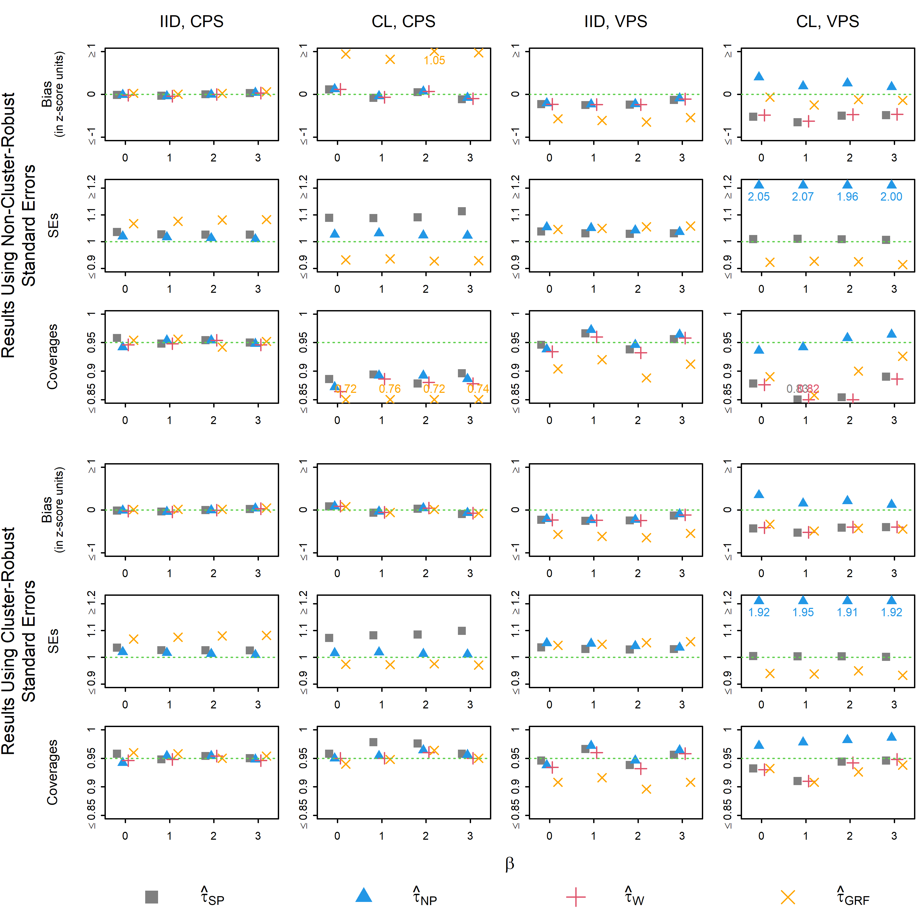
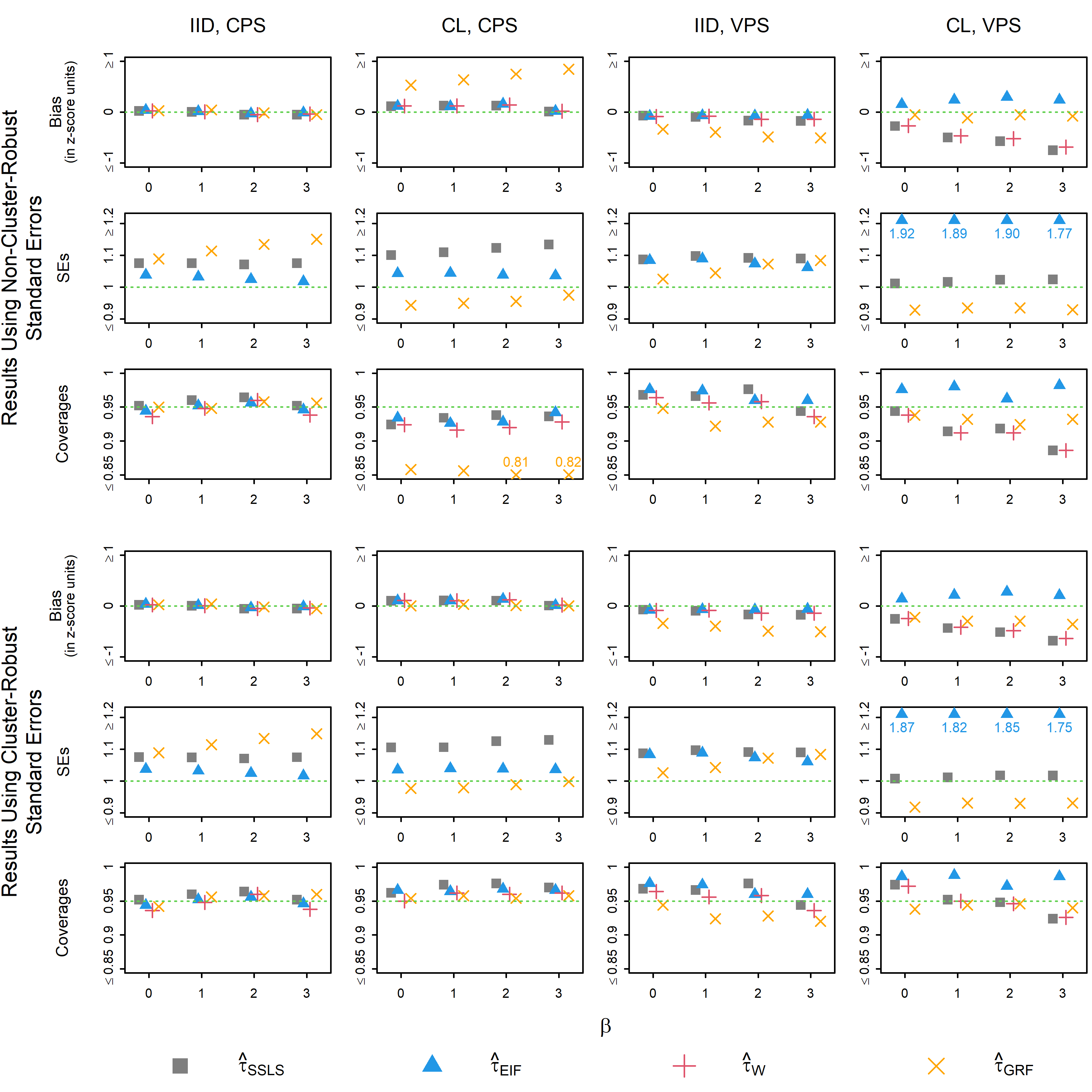
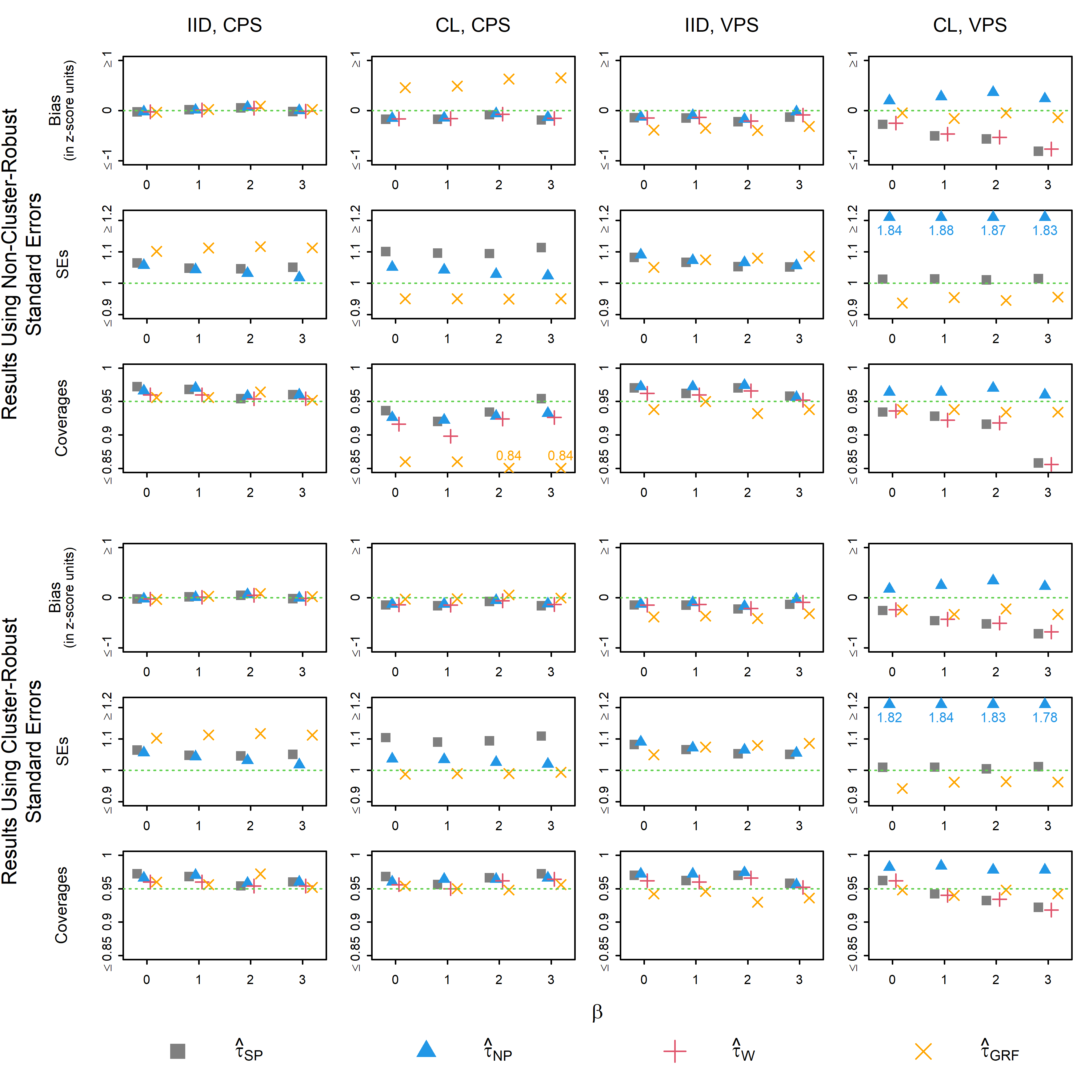
We only report the results associated with the first subgroup effect τ1\tau_{1}^{*}, but the results associated with other subgroup effects are similar; see Section A.3 of the Supplementary Material. We measure (a) bias (in zz-score units), (b) ratio of standard errors where the denominator of this ratio is the standard error of the combined estimator 𝝉^W\widehat{\bm{\tau}}_{\rm W}, and (c) coverage of 95% confidence intervals (CIs).

Figure 5.1 summarizes the result. In terms of bias, when β=0\beta=0 so that τ(𝐗i)\tau^{*}(\mathbf{X}_{i}) is constant within each subgroup and model PLM.Hom\mathcal{M}_{{{\rm PLM.Hom}}} holds, all estimators presented in Section 2 have negligible bias, as expected from our theoretical results. Similarly, when the propensity score is constant (i.e., Str.Exp\mathcal{M}_{{{\rm Str.Exp}}}), all estimators have little to no bias, even if β0\beta\neq 0. However, when neither the model PLM.Hom\mathcal{M}_{{{\rm PLM.Hom}}} nor Str.Exp\mathcal{M}_{{{\rm Str.Exp}}} hold, the semiparametric estimator and the combined estimator show some bias. On the other hand, the nonparametric estimator shows little to no bias in this setting.
Refer to caption
Figure 5.1: A Graphical Summary of the Simulation Results Associated with the First Groupwise Effect τ1\tau_{1}^{*}. Each column shows different combination of propensity score models (CPS, VPS) in equation (12) and whether the data is i.i.d. (IID) or clustered (CL). The top three rows use non-cluster-robust standard errors and the bottom three rows use cluster-robust standard errors. The xx-axes indicate the effect heterogeneity parameter β\beta with β=0\beta=0 satisfying model PLM.Hom\mathcal{M}_{{{\rm PLM.Hom}}}. The first and fourth rows show bias in z-score units. The second and fifth rows show ratio of standard errors where the denominator of the ratio is the standard error of the combined estimator 𝝉^W\widehat{\bm{\tau}}_{\rm W}. The third and sixth rows show coverage of 95% CIs. Green dashed lines are drawn for reference.

In terms of standard errors, as expected, the standard errors of the semiparametric estimator and the nonparametric estimator are always larger than the standard errors of the combined estimator across all scenarios, with the ratios of standard errors always exceeding 11. This also implies that the corresponding confidence intervals from the semiparametric estimator and the nonparametric estimator are larger than that from the combined estimator. For example, when β=0\beta=0 and the true propensity score model is the VPS model, the average length of confidence interval from the nonparametric estimator is roughly 1.84 times longer than that from the combined estimator. In general, when condition (SP) holds, inference based on the combined estimator is much more efficient than that based on the nonparametric or the semiparametric estimators.

For coverage, so long as the three estimators are consistent, using non-cluster-robust standard errors produce nominal coverage when the study units are not clustered. On the other hand, when the units are clustered, the three estimators using non-clustered standard errors may fail to achieve nominal coverage. This is most noticeable in the constant propensity score setting with clustered data where using cluster-robust standard errors help all three estimators achieve closer to nominal coverage compared to not using cluster-robust standard errors. Also, we see that using clustered standard errors when the underlying data is actually independent does not hurt coverage.

6 Applications: Early Childhood Longitudinal Study

6.1 Background, Defining Subgroups, and Clustering

We apply the methods discussed above to infer groupwise treatment effects of center-based pre-school programs on children’s academic achievement from the Early Childhood Longitudinal Study’s Kindergarten (ECLSK) Class of 1998-1999 dataset (Tourangeau et al., 2009). Briefly, the ECLSK dataset consists of children’s longitudinal histories from kindergarten through eighth grade in the United States. We consider that a child is treated (Ai=1)(A_{i}=1) if he/she received center-based care before entering kindergarten; otherwise, he/she is considered to be untreated (Ai=0A_{i}=0), which is usually parental care. We consider the outcome YiY_{i} as the standardized reading score of each child, which was measured during the 1998 Fall semester and after treatment assignment. The outcome is continuously distributed over an interval of [22.62,93.95][22.62,93.95]. As pre-treatment covariates, we include the following 8 variables in the analysis: census region (northeast/midwest/south/west), living location (central city/urban/rural), child’s gender (male/female), age, race/ethnicity (white/black/Hispanic/Asian/other), family type (intact/non-intact), parental education (has college graduate or not), and economic status. We restrict our analysis to 15,980 children with complete data on the outcome, treatment, and pre-treatment covariates. Finally, we remark that our analysis differs from that in Lee et al. (2021) where they focused on students’ math scores as the outcome and did not conduct a comparison between the three estimators presented in the paper.

Prior works (McCoy et al., 2016; Reardon, 2019) conjectured that the effect of early child development interventions on children’s academic and social skills are heterogeneous across region and location. Motivated from these works, we consider three subgroups defined by location to define groupwise effects. Also, since children’s performances in the same kindergarten are likely correlated, we account for this correlation by using the cluster-robust variances introduced in Section 4.2 where kindergartens are chosen as clusters. Also, to estimate the three nuisance functions ν\nu^{*}, μ\mu^{*}, and ee^{*}, we use the same procedure in Section 5.1 except we repeat cross-fitting 100 times.

6.2 Results

We first assessed covariate balance and overlap. For covariate balance, we compare the means of covariates in the treated and control groups before and after propensity score adjustment. We observe that covariate balance is dramatically improved after adjusting with the propensity score. We also visually found sufficient overlap between the treated and control groups; see Section A.4 of the Supplementary Material for details.

After checking covariate balance and overlap, we run the falsification test for the condition (SP). The falsification test statistics under H0g:τOV,g=τgH_{0g}:\tau_{{\rm OV},g}^{*}=\tau_{g}^{*} for g=1,2,3g=1,2,3 are (Z12,Z22,Z32)=(0.592,0.021,0.522)(Z_{1}^{2},Z_{2}^{2},Z_{3}^{2})=(0.592,0.021,0.522), which is significantly smaller than 3.84, the 95% percentile of a chi-square distribution with one degree of freedom. Therefore, the result suggests that the model SP\mathcal{M}_{{\rm SP}} is reasonable for all three subgroups.

Next, we estimated the groupwise effects and Table 6.1 summarizes the results. Overall, the three proposed estimators show very similar effect estimates. In particular, estimates obtained from the semiparametric estimator and the combined estimator are the same in Central City and Rural subgroups with weights w^Central City=w^Rural=1\widehat{w}_{\text{Central City}}=\widehat{w}_{\text{Rural}}=1. In the Urban subgroup, the estimate obtained from the combined estimator lies between the estimates obtained from the semiparametric estimator and the nonparametric estimator with a weight w^Urban=0.359\widehat{w}_{\text{Urban}}=0.359. Also, as expected, the standard error of the combined estimator was no larger than the standard errors from the semiparametric estimator or the nonparametric estimator. Notably, in the Urban subgroup, the standard error of the combined estimator is strictly smaller than those of the semiparametric and nonparametric estimators. The GRF-based estimators also yield similar effect sizes across the three subgroups, but are associated with larger standard errors compared to the combined estimator.

In terms of statistical significance at level α=0.05\alpha=0.05, the effect estimates from all the estimators are significant in the Urban and Central City subgroups whereas the effect estimates from all four estimators are insignificant in the Rural subgroup. The estimates remain statistically significant even after accounting for multiple testing across the three subgroups. Consequently, we conclude that the effect of center-based care before kindergarten on 1st year reading scores differs across living locations.

Subgroup Statistic 𝝉^SP\widehat{\bm{\tau}}_{\rm SP} 𝝉^NP\widehat{\bm{\tau}}_{\rm NP} 𝝉^W\widehat{\bm{\tau}}_{\rm W} 𝝉^GRF\widehat{\bm{\tau}}_{\rm GRF}
Central City Estimate 2.119 2.236 2.119 2.047
SE 0.292 0.344 0.292 0.333
95% CI (1.547,2.691) (1.561,2.912) (1.547,2.691) (1.395,2.700)
95% SCI (1.422,2.816) (1.414,3.059) (1.422,2.816) (1.253,2.842)
Urban Estimate 2.033 2.104 2.079 2.164
SE 0.325 0.321 0.319 0.370
95% CI (1.395,2.670) (1.476,2.733) (1.454,2.703) (1.438,2.890)
95% SCI (1.256,2.809) (1.338,2.870) (1.317,2.840) (1.280,3.049)
Rural Estimate 0.591 0.606 0.591 0.585
SE 0.361 0.379 0.361 0.366
95% CI (-0.115,1.298) (-0.137,1.349) (-0.115,1.298) (-0.132,1.303)
95% SCI (-0.270,1.452) (-0.300,1.511) (-0.270,1.452) (-0.289,1.459)
Table 6.1: Summary of the Data Analysis. Each row shows the statistics of interest for each subgroup. Each column shows the different estimators. SE, CI, and SCI stand for standard error, confidence interval, and simultaneous confidence interval, respectively.

7 Conclusion

This paper compares two different approaches of estimating groupwise treatment effects τg\tau_{g}^{*}, the nonparametric approach and the semiparametric approach. We state the assumptions underlying each approach, compare their statistical properties, and present a combined approach that has favorable efficiency properties in some settings. We also present some useful tools while using the estimators discussed in the paper, notably a falsification test for the semiparametric model and cluster-robust variance estimators when the study units’ data exhibit clustering. We demonstrate each approach through simulation and empirical studies.

For practice, our work suggests using the combined estimator if the model SP\mathcal{M}_{{\rm SP}} is satisfied by a study design (e.g., stratified experiment in Str.Exp\mathcal{M}_{{{\rm Str.Exp}}}) or is not severely violated based on the falsification test in Section 4.1. In this case, the combined estimator is the most efficient among the three estimators considered here. But, if the semiparametric model SP\mathcal{M}_{{\rm SP}} is not plausible, we recommend the nonparametric approach to estimate groupwise treatment effects.

Lastly, we end the paper by clarifying the relationship between the partially linear outcome model (PLM) and the proposed semiparametric model SP\mathcal{M}_{{\rm SP}}. Efficient estimation of 𝝉\bm{\tau}^{*} under the partially linear outcome model has been well-established for both homoskedastic and heteroskedastic error cases; see Robinson (1988), Chamberlain (1992), Robins et al. (1992), Newey (1994), Bhattacharya and Zhao (1997), Härdle et al. (2000), Li (2000), Robins and Rotnitzky (2001), and Ma et al. (2006) for related discussions. However, we again highlight that the semiparametric model SP\mathcal{M}_{{\rm SP}} is a strictly larger model than the partially linear model. Therefore, it is plausible that the efficient influence function for 𝝉\bm{\tau}^{*} under the partially linear outcome model (allowing for heteroskedasticity) and that under the semiparametric model SP\mathcal{M}_{{\rm SP}} can be different. For future research, it would be useful to derive the semiparametric efficiency bound for 𝝉\bm{\tau}^{*} under SP\mathcal{M}_{{\rm SP}} and construct an estimator of 𝝉\bm{\tau}^{*} that attains this bound rather than rely on the combined estimator to obtain a relatively efficient estimator.

Supplementary Material

This document contains supplementary materials for “A Groupwise Approach for Inferring Heterogeneous Treatment Effects in Causal Inference.” Section A discusses the details about the results of the main paper. Section B presents useful lemmas used in the proofs. Section C contains the proofs of the lemmas in Section B. Lastly, Section D contains the proof of the theorems in the main paper.

Appendix A Details of the Main Paper

A.1 A Visual Illustration of the Three Estimators

We provide some rationales for why the combined estimator can perform better than the other two. The influence functions of the estimators 𝝉^SP\widehat{\bm{\tau}}_{{\rm SP}} and 𝝉^NP\widehat{\bm{\tau}}_{{\rm NP}} (denoted by IFSP\textbf{IF}_{{\rm SP}} and IFNP\textbf{IF}_{{\rm NP}}, respectively) are valid in that the expectations of the products between these influence functions and the score function of the law are equal to the pathwise derivative of the groupwise effect, i.e.,

𝝉(η)η|η=η=E{IFSP(𝐎i)s(𝐎i)}=E{IFNP(𝐎i)s(𝐎i)},\displaystyle\frac{\partial\bm{\tau}(\eta)}{\partial\eta}\bigg|_{\eta=\eta^{*}}={\rm E}\big\{\textbf{IF}_{{\rm SP}}(\mathbf{O}_{i})\cdot s^{*}(\mathbf{O}_{i})\big\}={\rm E}\big\{\textbf{IF}_{{\rm NP}}(\mathbf{O}_{i})\cdot s^{*}(\mathbf{O}_{i})\big\}\ , (13)

where 𝝉(η)\bm{\tau}(\eta) is the groupwise effect under the parametric submodel of SP\mathcal{M}_{{\rm SP}} parametrized by 1-dimensional parameter η\eta which recovers the true law at η\eta^{*} and s(𝐎i)s^{*}(\mathbf{O}_{i}) is the corresponding score function of the observed data 𝐎i=(Yi,Ai,𝐗i)\mathbf{O}_{i}=(Y_{i},A_{i},\mathbf{X}_{i}) under model SP\mathcal{M}_{{\rm SP}}; see D.1 and D.2 for details. Therefore, both 𝝉^SP\widehat{\bm{\tau}}_{{\rm SP}} and 𝝉^NP\widehat{\bm{\tau}}_{{\rm NP}} are CAN estimators for the groupwise effect under model SP\mathcal{M}_{{\rm SP}}.

To become an efficient estimator under model SP\mathcal{M}_{{\rm SP}}, an influence function must belong to the tangent space of model SP\mathcal{M}_{{\rm SP}} (denoted by 𝒯SP\mathcal{T}_{{\rm SP}}; see (D.1) for the exact form). Since the laws in the semiparametric model SP\mathcal{M}_{{\rm SP}} must satisfy condition (SP), this imposes a restriction on the tangent space 𝒯SP\mathcal{T}_{{\rm SP}}, indicating that 𝒯SP\mathcal{T}_{{\rm SP}} is not equal to the entire Hilbert space of 𝐎\mathbf{O}. From some algebra, we can show that the two influence functions IFSP\textbf{IF}_{{\rm SP}} and IFNP\textbf{IF}_{{\rm NP}} do not belong to 𝒯SP\mathcal{T}_{{\rm SP}} in general; again, see D.1 and D.2 for details. This implies that there exist functions 𝒓SP\bm{r}_{{\rm SP}} and 𝒓NP\bm{r}_{{\rm NP}} that belong to the orthocomplement space of 𝒯SP\mathcal{T}_{{\rm SP}} (denoted by 𝒯SP\mathcal{T}_{{\rm SP}}^{\perp}) so that

IFSP(𝐎i)=IFSP(eff)(𝐎i)+𝒓SP(𝐎i),IFNP(𝐎i)=IFSP(eff)(𝐎i)+𝒓NP(𝐎i),𝒓SP,𝒓NP𝒯SP\displaystyle\textbf{IF}_{{\rm SP}}(\mathbf{O}_{i})=\textbf{IF}_{{\rm SP}}^{(\text{eff})}(\mathbf{O}_{i})+\bm{r}_{{\rm SP}}(\mathbf{O}_{i})\quad,\quad\textbf{IF}_{{\rm NP}}(\mathbf{O}_{i})=\textbf{IF}_{{\rm SP}}^{(\text{eff})}(\mathbf{O}_{i})+\bm{r}_{{\rm NP}}(\mathbf{O}_{i})\quad,\quad\bm{r}_{{\rm SP}},\bm{r}_{{\rm NP}}\in\mathcal{T}_{{\rm SP}}^{\perp}

where IFSP(eff)\textbf{IF}_{{\rm SP}}^{(\text{eff})} is the efficient influence function for 𝝉\bm{\tau}^{*} under model SP\mathcal{M}_{{\rm SP}}. As a result, any linear combinations of the two influence functions IFSP(𝐎i)\textbf{IF}_{{\rm SP}}(\mathbf{O}_{i}) and IFNP(𝐎i)\textbf{IF}_{{\rm NP}}(\mathbf{O}_{i}) must have a form of

IFW(𝐎i):\displaystyle\textbf{IF}_{{\rm W}}(\mathbf{O}_{i}): =WIFSP(𝐎i)+(IW)IFNP(𝐎i)\displaystyle\hskip-2.84544pt=W\cdot\textbf{IF}_{{\rm SP}}(\mathbf{O}_{i})+(I-W)\cdot\textbf{IF}_{{\rm NP}}(\mathbf{O}_{i})
=IFSP(eff)(𝐎i)+W𝒓SP(𝐎i)+(IW)𝒓NP(𝐎i)=:𝒓W(𝐎i)\displaystyle=\textbf{IF}_{{\rm SP}}^{(\text{eff})}(\mathbf{O}_{i})+\underbrace{W\cdot\bm{r}_{{\rm SP}}(\mathbf{O}_{i})+(I-W)\cdot\bm{r}_{{\rm NP}}(\mathbf{O}_{i})}_{=:\bm{r}_{{\rm W}}(\mathbf{O}_{i})}

where W=diag(w1,,wG)W=\text{diag}(w_{1},\ldots,w_{G}) is a diagonal weight matrix. Here, the weighted residual function rW(𝐎i)r_{{\rm W}}(\mathbf{O}_{i}) also belongs to the tangent space 𝒯SP\mathcal{T}_{{\rm SP}}, and the weighted influence function IFW\textbf{IF}_{{\rm W}} also satisfies the differentiable parameter condition (13), indicating that the estimator based on the weighted influence function (which is in fact the combined estimator 𝝉^W\widehat{\bm{\tau}}_{{\rm W}}) is also CAN for the groupwise effect 𝝉\bm{\tau}^{*}.

Based on the results above, we find that three regular, asymptotic linear estimators 𝝉^SP\widehat{\bm{\tau}}_{{\rm SP}}, 𝝉^NP\widehat{\bm{\tau}}_{{\rm NP}}, and 𝝉^W\widehat{\bm{\tau}}_{{\rm W}}) are CAN for 𝝉\bm{\tau}^{*} with the corresponding influence functions IFSP\textbf{IF}_{{\rm SP}}, IFNP\textbf{IF}_{{\rm NP}}, and IFW\textbf{IF}_{{\rm W}}, respectively. If the first two influence functions are associated with non-zero residual functions 𝒓SP\bm{r}_{{\rm SP}} and 𝒓NP\bm{r}_{{\rm NP}}, none of the estimators is efficient. Consequently, if the weight matrix WW is chosen appropriately, the weighted residual 𝒓W\bm{r}_{{\rm W}} may have a smaller variance than 𝒓SP\bm{r}_{{\rm SP}} and 𝒓NP\bm{r}_{{\rm NP}}. In fact, the combined estimator 𝝉^W\widehat{\bm{\tau}}_{{\rm W}} is constructed to make the variance of 𝒓W\bm{r}_{{\rm W}} as small as possible. Figure A.1 depicts how the weighted influence function (and the corresponding estimator) can be more efficient than the other two influence functions (and the corresponding estimators).
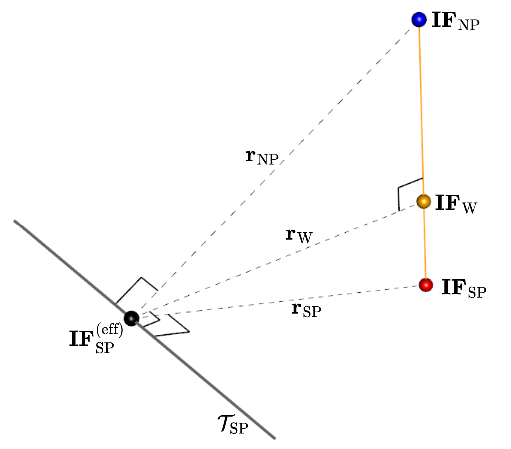
Refer to caption
Figure A.1: An Illustration of the Influence Functions. Black, blue, red, and orange dots depict IFSP(eff)\textbf{IF}_{{\rm SP}}^{(\text{eff})}, IFNP\textbf{IF}_{{\rm NP}}, IFSP\textbf{IF}_{{\rm SP}}, and IFW\textbf{IF}_{{\rm W}}, respectively. The gray line depicts the tangent space 𝒯SP\mathcal{T}_{{\rm SP}}. Three dashed lines depict the residual functions 𝒓NP\bm{r}_{{\rm NP}}, 𝒓SP\bm{r}_{{\rm SP}}, and 𝒓W\bm{r}_{{\rm W}}. The orange line is the collection of the weighted influence functions of the form WIFSP+(IW)IFNPW\cdot\textbf{IF}_{{\rm SP}}+(I-W)\cdot\textbf{IF}_{{\rm NP}}. Black corners ( .A¯|\overline{{\color[rgb]{1,1,1}{.A}}}\hskip-1.42271pt\big| ) depicts that two segments are orthogonal.

A.2 Details of the Superlearner Library and Cross-fitting Procedure

We include the following methods and the corresponding R packages in our super learner library: linear regression via glm, lasso/elastic net via glmnet (Friedman et al., 2010), spline via earth (Friedman, 1991) and polspline (Kooperberg, 2020), generalized additive model via gam (Hastie and Tibshirani, 1986), boosting via xgboost (Chen and Guestrin, 2016) and gbm (Friedman, 2001), random forest via ranger (Wright and Ziegler, 2017), and neural net via RSNNS (Bergmeir and Benítez, 2012).

Let 𝝉^SP(s)\widehat{\bm{\tau}}_{\rm SP}^{(s)} and 𝝉^NP(s)\widehat{\bm{\tau}}_{\rm NP}^{(s)} be the estimators from ssth cross-fitting procedure and let Σ^SP(s)\widehat{\Sigma}_{\rm SP}^{(s)}, Σ^NP(s)\widehat{\Sigma}_{\rm NP}^{(s)}, and Σ^SP,NP(s)\widehat{\Sigma}_{{\rm SP},{\rm NP}}^{(s)} be the associated variance estimates. Afterwards, we compute the component-wise medians of the estimators, i.e.

(𝝉^SPmed𝝉^NPmed)=medians=1,,S(𝝉^SP(s)𝝉^NP(s)).\displaystyle\begin{pmatrix}\widehat{\bm{\tau}}_{\rm SP}^{\text{med}}\\ \widehat{\bm{\tau}}_{\rm NP}^{\text{med}}\end{pmatrix}=\median_{s=1,\ldots,S}\begin{pmatrix}\widehat{\bm{\tau}}_{\rm SP}^{(s)}\\ \widehat{\bm{\tau}}_{\rm NP}^{(s)}\end{pmatrix}\ .

Also, the following variance estimators are used:

[Σ^SPmedΣ^SP,NPmedΣ^SP,NPmed,Σ^NPmed]=medians=1,,S[[Σ^SP(s)Σ^SP,NP(s)Σ^SP,NP(s),Σ^NP(s)]+(𝝉^SP(s)𝝉^SPmed𝝉^NP(s)𝝉^NPmed)2]\displaystyle\begin{bmatrix}\widehat{\Sigma}_{\rm SP}^{\text{med}}&\widehat{\Sigma}_{{\rm SP},{\rm NP}}^{\text{med}}\\ \widehat{\Sigma}_{{\rm SP},{\rm NP}}^{\text{med},\intercal}&\widehat{\Sigma}_{\rm NP}^{\text{med}}\end{bmatrix}=\median_{s=1,\ldots,S}\left[\begin{bmatrix}\widehat{\Sigma}_{\rm SP}^{(s)}&\widehat{\Sigma}_{{\rm SP},{\rm NP}}^{(s)}\\ \widehat{\Sigma}_{{\rm SP},{\rm NP}}^{(s),\intercal}&\widehat{\Sigma}_{\rm NP}^{(s)}\end{bmatrix}+\begin{pmatrix}\widehat{\bm{\tau}}_{\rm SP}^{(s)}-\widehat{\bm{\tau}}_{\rm SP}^{\text{med}}\\ \widehat{\bm{\tau}}_{\rm NP}^{(s)}-\widehat{\bm{\tau}}_{\rm NP}^{\text{med}}\end{pmatrix}^{\otimes 2}\right]

where the median is evaluated based on the matrix 2-norm. As shown in Theorem 3.3 of Chernozhukov et al. (2018), the established results extend to the median-adjusted estimators.

A.3 Additional Results of the Simulation

Refer to caption
Figure A.2: Graphical Summary of the Simulation Results Associated with the Second Groupwise Effect τ2\tau_{2}^{*}. Each column shows a different combination of propensity score (PS) models in (12) in the main paper and clustering. The top three rows use non-cluster-robust standard errors and the bottom three rows use cluster-robust standard errors. The xx-axes of the plots indicate the effect heterogeneity parameter β\beta. The first and fourth rows show bias in z-score units. The second and fifth rows show the ratio of standard errors where the denominator is the combined estimator’s standard error. The third and sixth rows show coverage of 95% CIs. Green dashed lines are drawn for reference.
Refer to caption
Figure A.3: Graphical Summary of the Simulation Results Associated with the Third Groupwise Effect τ3\tau_{3}^{*}. Each column shows a different combination of propensity score (PS) models in (12) in the main paper and clustering. The top three rows use non-cluster-robust standard errors and the bottom three rows use cluster-robust standard errors. The xx-axes of the plots indicate the effect heterogeneity parameter β\beta. The first and fourth rows show bias in z-score units. The second and fifth rows show the ratio of standard errors where the denominator is the combined estimator’s standard error. The third and sixth rows show coverage of 95% CIs. Green dashed lines are drawn for reference.
Refer to caption
Figure A.4: Graphical Summary of the Simulation Results Associated with the Fourth Groupwise Effect τ4\tau_{4}^{*}. Each column shows a different combination of propensity score (PS) models in (12) in the main paper and clustering. The top three rows use non-cluster-robust standard errors and the bottom three rows use cluster-robust standard errors. The xx-axes of the plots indicate the effect heterogeneity parameter β\beta. The first and fourth rows show bias in z-score units. The second and fifth rows show the ratio of standard errors where the denominator is the combined estimator’s standard error. The third and sixth rows show coverage of 95% CIs. Green dashed lines are drawn for reference.

A.4 Assessment of Assumptions (A2) and (A3) in the Main Paper

To assess assumption (A2), we assessed covariate balance as follows. Let X~iPS.nonAdj\widetilde{X}_{i}^{{\rm PS.nonAdj}} and X~iPS.Adj\widetilde{X}_{i}^{{\rm PS.Adj}} be

X~ipPS.nonAdj=AiXip1Ni=1NAi(1Ai)Xip1Ni=1N(1Ai),X~ipPS.Adj=AiXipe^Med(𝐗i)(1Ai)Xip1e^Med(𝐗i),\displaystyle\widetilde{X}_{ip}^{{\rm PS.nonAdj}}=\frac{A_{i}X_{ip}}{\frac{1}{N}\sum_{i=1}^{N}A_{i}}-\frac{(1-A_{i})X_{ip}}{\frac{1}{N}\sum_{i=1}^{N}(1-A_{i})}\ ,\ \widetilde{X}_{ip}^{{\rm PS.Adj}}=\frac{A_{i}X_{ip}}{\widehat{e}^{\rm Med}(\mathbf{X}_{i})}-\frac{(1-A_{i})X_{ip}}{1-\widehat{e}^{\rm Med}(\mathbf{X}_{i})}\ ,

where XipX_{ip} is the ppth covariate of unit ii and e^Med(𝐗i)\widehat{e}^{\rm Med}(\mathbf{X}_{i}) is the median value of the propensity score estimate obtained from 100 sample split. To address the correlation within each cluster, we consider the following generalized linear mixed effect models (GLMMs):

X~c(j),pPS.nonAdjμpPS.nonAdj+ucpPS.nonAdj+ϵc(j),pPS.nonAdj,X~c(j),pPS.AdjμpPS.Adj+ucpPS.Adj+ϵc(j),pPS.Adj\displaystyle\widetilde{X}_{c(j),p}^{{\rm PS.nonAdj}}\sim\mu_{p}^{{\rm PS.nonAdj}}+u_{cp}^{{\rm PS.nonAdj}}+\epsilon_{c(j),p}^{{\rm PS.nonAdj}}\ ,\ \widetilde{X}_{c(j),p}^{{\rm PS.Adj}}\sim\mu_{p}^{{\rm PS.Adj}}+u_{cp}^{{\rm PS.Adj}}+\epsilon_{c(j),p}^{{\rm PS.Adj}}

where ucpu_{cp} is the cluster-level random effect for cluster cc and ϵc(j),p\epsilon_{c(j),p} is the unit-level error for the jjth unit in cluster cc. Using the GLMMs, we test H0pPS.nonAdj:μpPS.nonAdj=0H_{0p}^{{\rm PS.nonAdj}}:\mu_{p}^{{\rm PS.nonAdj}}=0 and H0pPS.Adj:μpPS.nonAdj=0H_{0p}^{{\rm PS.Adj}}:\mu_{p}^{{\rm PS.nonAdj}}=0. For H0pPS.nonAdjH_{0p}^{{\rm PS.nonAdj}}, a larger (smaller) test statistic suggests that covariate balance is achieved (violated) without adjusting the propensity score. Similarly, for H0pPS.AdjH_{0p}^{{\rm PS.Adj}}, a larger (smaller) test statistic suggests that covariate balance is achieved (violated) with adjusting the propensity score.

Table A.1 summarizes covariate balance assessment. We find that covariate balance is dramatically improved after adjusting the propensity score and there is no significant Wald statistics that rejects H0pPS.AdjH_{0p}^{{\rm PS.Adj}} other than socioeconomic status. This concludes assumption (A2) is not severely violated.

Variable H0pPS.nonAdjH_{0p}^{{\rm PS.nonAdj}} H0pPS.AdjH_{0p}^{{\rm PS.Adj}} Variable H0pPS.nonAdjH_{0p}^{{\rm PS.nonAdj}} H0pPS.AdjH_{0p}^{{\rm PS.Adj}}
Census Region = Northeast -0.71 -1.07 Race = Asian -2.81 -1.89
Census Region = South 1.88 0.46 Race = Black 6.47 0.98
Census Region = West -4.87 -1.53 Race = White 2.11 0.75
Location = City -0.8 -0.52 Race = Hispanic -7.42 -1.13
Location = Rural -3.62 -1.46 Family = Intact -1.76 -0.46
Gender = Male -0.59 -0.29 Parental Education = College Graduate 7.26 0.74
Age 2.25 0.98 Socioeconomic Status 16.5 2.59
Table A.1: Result of Covariate Balance Assessment. The numbers show the Wald statistics obtained from testing H0pPS.nonAdjH_{0p}^{{\rm PS.nonAdj}} and H0pPS.AdjH_{0p}^{{\rm PS.Adj}}.

Next, to assess assumption (A3), we plot e^Med(𝐗i)\widehat{e}^{\rm Med}(\mathbf{X}_{i}) according to the treatment status. Figure A.5 shows the result and the overlap assumption is not severely violated.
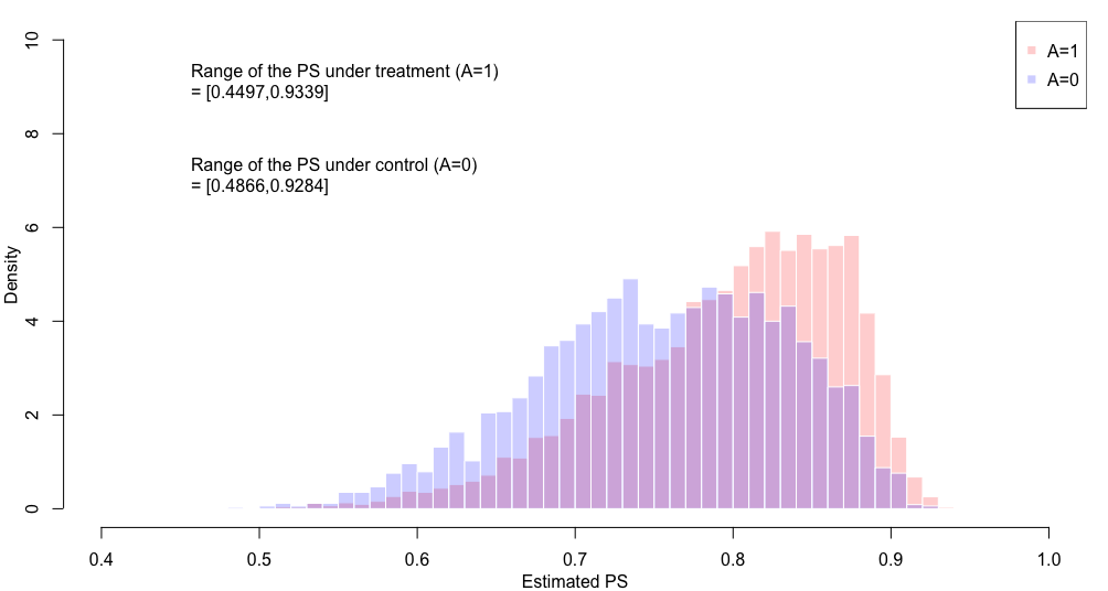
Refer to caption
Figure A.5: Histograms of the Propensity Score Estimates.

Appendix B Lemma

We introduce useful lemmas for the proof of theorems in the main paper.

Lemma B.1.

Let 𝐔\mathbf{U} and 𝐕\mathbf{V} be the random vectors. Then,

E(𝐔𝐕)2E(𝐔𝐕2)E(𝐔22)E(𝐕22).\displaystyle\big\|E(\mathbf{U}\mathbf{V}^{\intercal})\big\|_{2}\leq{\rm E}\big(\|\mathbf{U}\mathbf{V}^{\intercal}\|_{2}\big)\leq\sqrt{{\rm E}\big(\|\mathbf{U}\|_{2}^{2}\big){\rm E}\big(\|\mathbf{V}\|_{2}^{2}\big)}\ .

Furthermore, suppose 𝐔\mathbf{U} is a bounded random vector, i.e., 𝐔2M\lVert\mathbf{U}\rVert_{2}\leq M for some MM. Then,

E(𝐔𝐕2)ME(𝐕2).\displaystyle{\rm E}\big(\lVert\mathbf{U}\mathbf{V}^{\intercal}\rVert_{2}\big)\leq M\cdot{\rm E}\big(\lVert\mathbf{V}\rVert_{2}\big)\ .

Also, for r1r\geq 1, we have

E(𝐔𝐕2r)E(𝐔22r)E(𝐕22r).\displaystyle{\rm E}\big(\lVert\mathbf{U}\mathbf{V}^{\intercal}\rVert_{2}^{r}\big)\leq\sqrt{{\rm E}\big(\|\mathbf{U}\|_{2}^{2r}\big){\rm E}\big(\|\mathbf{V}\|_{2}^{2r}\big)}\ .
Proof.

The proof is in Section C.1. ∎

Lemma B.2.

(Chernozhukov et al., 2018) Let aNa_{N} be a sequence of positive numbers for N=1,2,N=1,2,\ldots. If 𝐗N=OP(aN)\lVert\mathbf{X}_{N}\rVert=O_{P}(a_{N}) conditional on 𝐘N\mathbf{Y}_{N}, then 𝐗N=OP(aN)\lVert\mathbf{X}_{N}\rVert=O_{P}(a_{N}) unconditionally.

Proof.

The proof is in Section C.2. ∎

Lemma B.3.

Let 𝐕i={Aie(𝐗i)}𝐈(𝐗i)\mathbf{V}_{i}^{*}=\{A_{i}-e^{*}(\mathbf{X}_{i})\}\mathbf{I}(\mathbf{X}_{i}), Zi=Yiν(𝐗i)Z_{i}^{*}=Y_{i}-\nu^{*}(\mathbf{X}_{i}), 𝐕^i(k)={Aie(k)(𝐗i)}𝐈(𝐗i)\widehat{\mathbf{V}}_{i}^{(-k)}=\{A_{i}-e^{(-k)}(\mathbf{X}_{i})\}\mathbf{I}(\mathbf{X}_{i}), Z^i(k)=Yiν(k)(𝐗i)\widehat{Z}_{i}^{(-k)}=Y_{i}-\nu^{(-k)}(\mathbf{X}_{i}), ξi=Zi𝐕i,𝝉OV\xi_{i}=Z_{i}^{*}-\mathbf{V}_{i}^{*,\intercal}\bm{\tau}_{\rm OV}^{*}, and ξi(k)=Z^i(k)𝐕^i(k),𝝉OV\xi_{i}^{(-k)}=\widehat{Z}_{i}^{(-k)}-\widehat{\mathbf{V}}_{i}^{(-k),\intercal}\bm{\tau}_{\rm OV}^{*}. Under Assumptions (A1)-(A4) and Assumptions 3.1 and 3.2 in the main paper, the following conditions hold.

  1. (a)

    E(𝐕i,ξi)=0{\rm E}(\mathbf{V}_{i}^{{}^{*,\intercal}}\xi_{i})=0.

  2. (b)

    𝐕iP,4\big\|\mathbf{V}_{i}^{*}\big\|_{P,4}, 𝐕^i(k)P,4\big\|\widehat{\mathbf{V}}_{i}^{(-k)}\big\|_{P,4}, 𝐕i,ξiP,2\big\|\mathbf{V}_{i}^{*,\intercal}\xi_{i}\big\|_{P,2}, and E(ξiξi|𝐕i){\rm E}\big(\xi_{i}\xi_{i}^{\intercal}\,|\,\mathbf{V}_{i}^{*}\big) are bounded.

  3. (c)

    E(𝐕i𝐕i,){\rm E}\big(\mathbf{V}_{i}^{*}\mathbf{V}_{i}^{*,\intercal}\big) and E{𝐕i(k)𝐕i(k),|kC}{\rm E}\big\{\mathbf{V}_{i}^{(-k)}\mathbf{V}_{i}^{(-k),\intercal}\,|\,\mathcal{I}_{k}^{C}\big\} are full rank.

  4. (d)

    Z^i(k)ZiP,2=oP(1)\|\widehat{Z}_{i}^{(-k)}-Z_{i}^{*}\|_{P,2}=o_{P}(1) and 𝐕^i(k)𝐕iP,2=oP(1)\|\widehat{\mathbf{V}}_{i}^{(-k)}-\mathbf{V}_{i}^{*}\|_{P,2}=o_{P}(1) as NN\rightarrow\infty.

  5. (e)

    NE{𝐕^i(k),ξi(k)|kC}2=oP(1)\sqrt{N}\,\big\|{\rm E}\big\{\widehat{\mathbf{V}}_{i}^{(-k),\intercal}\xi_{i}^{(-k)}\,\big|\,\mathcal{I}_{k}^{C}\big\}\big\|_{2}=o_{P}(1) and 𝐕^i(k),ξi(k)𝐕i,ξiP,2=oP(1)\big\|\widehat{\mathbf{V}}_{i}^{(-k),\intercal}\xi_{i}^{(-k)}-\mathbf{V}_{i}^{*,\intercal}\xi_{i}\big\|_{P,2}=o_{P}(1) as NN\to\infty.

Proof.

The proof is in Section C.3. ∎

Lemma B.4.

Let ={P|P(𝐎i) satisfies Assumptions (A1)-(A4) in the main maper}\mathcal{M}=\big\{P\,|\,P(\mathbf{O}_{i})\text{ satisfies Assumptions (A1)-(A4) in the main maper}\}. The efficient influence function of 𝝉\bm{\tau}^{*} in \mathcal{M} is ϕ(𝐎i)=(ϕ1(𝐎i),,ϕG(𝐎i))\bm{\phi}(\mathbf{O}_{i})=\big(\phi_{1}(\mathbf{O}_{i}),\ldots,\phi_{G}(\mathbf{O}_{i})\big)^{\intercal} where

ϕg(𝐎i)=𝟙{M(𝐗i)=g}{φ(𝐎i)τg}pg,pg=P{M(𝐗i)=g},\displaystyle\phi_{g}(\mathbf{O}_{i})=\frac{\mathbbm{1}\big\{M(\mathbf{X}_{i})=g\big\}\big\{\varphi(\mathbf{O}_{i})-\tau_{g}^{*}\big\}}{p_{g}^{*}}\ ,\ p_{g}^{*}=P\big\{M(\mathbf{X}_{i})=g\big\}\ ,
φ(𝐎i)=Ai{Yiμ(1,𝐗i)}e(𝐗i)(1Ai){Yiμ(0,𝐗i)}1e(𝐗i)+μ(1,𝐗i)μ(0,𝐗i).\displaystyle\varphi(\mathbf{O}_{i})=\frac{A_{i}\big\{Y_{i}-\mu^{*}(1,\mathbf{X}_{i})\big\}}{e^{*}(\mathbf{X}_{i})}-\frac{(1-A_{i})\big\{Y_{i}-\mu^{*}(0,\mathbf{X}_{i})\big\}}{1-e^{*}(\mathbf{X}_{i})}+\mu^{*}(1,\mathbf{X}_{i})-\mu^{*}(0,\mathbf{X}_{i})\ .

Therefore, the semiparametric efficiency bound of 𝝉\bm{\tau}^{*} is ΣNP=diag(σNP,12,,σNP,G2)\Sigma_{\rm NP}={\rm diag}(\sigma_{{\rm NP},1}^{2},\ldots,\sigma_{{\rm NP},G}^{2}) where

σNP,g2=E[{φ(𝐎i)τg}2𝟙{M(𝐗i)=g}](pg)2\displaystyle\sigma_{{\rm NP},g}^{2}=\frac{{\rm E}\big[\big\{\varphi(\mathbf{O}_{i})-\tau_{g}^{*}\big\}^{2}\mathbbm{1}\{M(\mathbf{X}_{i})=g\}\big]}{(p_{g}^{*})^{2}}

Moreover, the estimated slope coefficients from regressing φ(𝐎i)\varphi(\mathbf{O}_{i}) on 𝐈(𝐗i)\mathbf{I}(\mathbf{X}_{i}) without the intercept term achieve the bound.

Proof.

The proof is in Section C.4. ∎

Lemma B.5.

Let 𝐕i=𝐕^i(k)=𝐈(𝐗i)\mathbf{V}_{i}^{*}=\widehat{\mathbf{V}}_{i}^{(-k)}=\mathbf{I}(\mathbf{X}_{i}), Zi=φ(𝐎i)Z_{i}^{*}=\varphi^{*}(\mathbf{O}_{i}), Z^i(k)=φ^(k)(𝐎i)\widehat{Z}_{i}^{(-k)}=\widehat{\varphi}^{(-k)}(\mathbf{O}_{i}), ξi=ϵi=Zi𝐕i,𝝉\xi_{i}=\epsilon_{i}=Z_{i}^{*}-\mathbf{V}_{i}^{*,\intercal}\bm{\tau}^{*}, and ξi(k)=ϵi(k)=Z^i(k)𝐕^i(k),𝝉\xi_{i}^{(-k)}=\epsilon_{i}^{(-k)}=\widehat{Z}_{i}^{(-k)}-\widehat{\mathbf{V}}_{i}^{(-k),\intercal}\bm{\tau}^{*}. Under Assumptions (A1)-(A4) and Assumptions 3.1 and 3.3 in the main paper, the conditions in Lemma B.3 hold.

Proof.

The proof is in Section C.5. ∎

Lemma B.6.

Let us denote

𝐕i=[𝐕SP,i𝐕NP,i]=[{Aie(𝐗i)𝐈(𝐗i)𝐈(𝐗i)]\displaystyle\mathbf{V}_{i}^{*}=\begin{bmatrix}\mathbf{V}_{{\rm SP},i}^{*}\\ \mathbf{V}_{{\rm NP},i}^{*}\end{bmatrix}=\begin{bmatrix}\{A_{i}-e^{*}(\mathbf{X}_{i})\mathbf{I}(\mathbf{X}_{i})\\ \mathbf{I}(\mathbf{X}_{i})\end{bmatrix} 𝐕^i(k)=[𝐕^SP,i(k)𝐕^NP,i(k)]=[{Aie^(k)(𝐗i)𝐈(𝐗i)𝐈(𝐗i)]\displaystyle\widehat{\mathbf{V}}_{i}^{(-k)}=\begin{bmatrix}\widehat{\mathbf{V}}_{{\rm SP},i}^{(-k)}\\ \widehat{\mathbf{V}}_{{\rm NP},i}^{(-k)}\end{bmatrix}=\begin{bmatrix}\{A_{i}-\widehat{e}^{(-k)}(\mathbf{X}_{i})\mathbf{I}(\mathbf{X}_{i})\\ \mathbf{I}(\mathbf{X}_{i})\end{bmatrix}
𝐙i=[ZSP,iZNP,i]=[Yiν(𝐗i)φ(𝐎i)]\displaystyle\mathbf{Z}_{i}^{*}=\begin{bmatrix}Z_{{\rm SP},i}^{*}\\ Z_{{\rm NP},i}^{*}\end{bmatrix}=\begin{bmatrix}Y_{i}-\nu^{*}(\mathbf{X}_{i})\\ \varphi^{*}(\mathbf{O}_{i})\end{bmatrix} 𝐙^i(k)=[Z^SP,i(k)Z^NP,i(k)]=[Yiν^(k)(𝐗i)φ^(k)(𝐎i)]\displaystyle\widehat{\mathbf{Z}}_{i}^{(-k)}=\begin{bmatrix}\widehat{Z}_{{\rm SP},i}^{(-k)}\\ \widehat{Z}_{{\rm NP},i}^{(-k)}\end{bmatrix}=\begin{bmatrix}Y_{i}-\widehat{\nu}^{(-k)}(\mathbf{X}_{i})\\ \widehat{\varphi}^{(-k)}(\mathbf{O}_{i})\end{bmatrix}
𝝃i=[ξSP,iξNP,i]=[ZSP,i𝐕SP,i,𝝉OVZSP,i𝐕SP,i,𝝉]\displaystyle\bm{\xi}_{i}=\begin{bmatrix}\xi_{{\rm SP},i}\\ \xi_{{\rm NP},i}\end{bmatrix}=\begin{bmatrix}{Z}_{{\rm SP},i}^{*}-{\mathbf{V}}_{{\rm SP},i}^{*,\intercal}\bm{\tau}_{{\rm OV}}^{*}\\ {Z}_{{\rm SP},i}^{*}-{\mathbf{V}}_{{\rm SP},i}^{*,\intercal}\bm{\tau}^{*}\end{bmatrix} 𝝃^i(k)=[ξ^SP,i(k)ξ^NP,i(k)]=[Z^SP,i(k)𝐕^SP,i(k),𝝉OVZ^SP,i(k)𝐕^SP,i(k),𝝉]\displaystyle\widehat{\bm{\xi}}_{i}^{(-k)}=\begin{bmatrix}\widehat{\xi}_{{\rm SP},i}^{(-k)}\\ \widehat{\xi}_{{\rm NP},i}^{(-k)}\end{bmatrix}=\begin{bmatrix}\widehat{Z}_{{\rm SP},i}^{(-k)}-\widehat{\mathbf{V}}_{{\rm SP},i}^{(-k),\intercal}\bm{\tau}_{{\rm OV}}^{*}\\ \widehat{Z}_{{\rm SP},i}^{(-k)}-\widehat{\mathbf{V}}_{{\rm SP},i}^{(-k),\intercal}\bm{\tau}^{*}\end{bmatrix}

Under Assumptions (A1)-(A4) and Assumptions 3.1, 3.2, and 3.3 in the main paper, the conditions in Lemma B.3 hold.

Proof.

The proof is in Section C.6. ∎

Lemma B.7.

Let ΣSP\Sigma_{\rm SP}, ΣNP\Sigma_{\rm NP}, and ΣSP,NP\Sigma_{{\rm SP},{\rm NP}} be the asymptotic variances of 𝝉^SP\widehat{\bm{\tau}}_{\rm SP}, 𝝉^NP\widehat{\bm{\tau}}_{\rm NP}, and the asymptotic covariance of 𝝉^SP\widehat{\bm{\tau}}_{\rm SP} and 𝝉^NP\widehat{\bm{\tau}}_{\rm NP}, respectively. Suppose model (PLM) in the main paper is true and the error ϵi\epsilon_{i} is homoscedastic within each subgroup (i.e., Var(ϵi|Ai,𝐗i)=σϵ,g2{\rm Var}(\epsilon_{i}\,|\,A_{i},\mathbf{X}_{i})=\sigma_{\epsilon,g}^{2} for all (Ai,𝐗i)(A_{i},\mathbf{X}_{i}) satisfying M(𝐗i)=gM(\mathbf{X}_{i})=g). Then, ΣNPΣSP\Sigma_{\rm NP}-\Sigma_{\rm SP} is positive semi-definite and ΣSP,NP=ΣSP\Sigma_{{\rm SP},{\rm NP}}=\Sigma_{\rm SP}. Moreover, if the propensity score e(𝐗i)e^{*}(\mathbf{X}_{i}) is constant within each subgroup (i.e., condition (b) of Theorem 3.2 in the main paper), we have ΣNP=ΣSP\Sigma_{\rm NP}=\Sigma_{\rm SP}.

Proof.

The proof is in Section C.7. ∎

Appendix C Proof of Lemmas in Section B

C.1 Proof of Lemma B.1

For the first result, we observe that the matrix spectral norm is convex and induced by the vector 22-norm. As a result, the Jensen’s inequality, the submultiplicavity of the spectral norm, and Hölder’s inequality gives the result

𝐔𝐕𝑑P2\displaystyle\bigg\|\int\mathbf{U}\mathbf{V}^{\intercal}dP\bigg\|_{2} 𝐔𝐕2𝑑P𝐔2𝐕2𝑑P𝐔22𝑑P𝐕22𝑑P.\displaystyle\leq\int\lVert\mathbf{U}\mathbf{V}^{\intercal}\rVert_{2}\,dP\leq\int\lVert\mathbf{U}\rVert_{2}\lVert\mathbf{V}\rVert_{2}\,dP\leq\sqrt{\int\lVert\mathbf{U}\rVert_{2}^{2}\,dP\int\lVert\mathbf{V}\rVert_{2}^{2}\,dP}\ . (14)

Here, PP is the law of (𝐔,𝐕)(\mathbf{U},\mathbf{V}). The second result is trivial by replacing 𝐔2\|\mathbf{U}\|_{2} with MM in the third integral of (14). The last result holds via analogous steps:

𝐔𝐕2r𝑑P𝐔2r𝐕2r𝑑P𝐔22r𝑑P𝐕22r𝑑P.\displaystyle\int\lVert\mathbf{U}\mathbf{V}^{\intercal}\rVert_{2}^{r}\,dP\leq\int\lVert\mathbf{U}\rVert_{2}^{r}\lVert\mathbf{V}\rVert_{2}^{r}\,dP\leq\sqrt{\int\lVert\mathbf{U}\rVert_{2}^{2r}dP\int\lVert\mathbf{V}\rVert_{2}^{2r}\,dP}\ .

C.2 Proof of Lemma B.2

See Lemma 6.1 of Chernozhukov et al. (2018).

C.3 Proof of Lemma B.3

We proof the claim of the lemma in following Step 1Step 6.

Step 1: We find

E[ϵi{Aie(𝐗i)}𝐈(𝐗i)]=E[𝐕i{Zi𝐕i,𝝉OV}]=E(𝐕iZi)E(𝐕i𝐕i,)𝝉OV.\displaystyle{\rm E}\big[\epsilon_{i}\{A_{i}-e^{*}(\mathbf{X}_{i})\}\mathbf{I}(\mathbf{X}_{i})\big]={\rm E}\big[\mathbf{V}_{i}^{*}\big\{Z_{i}^{*}-\mathbf{V}_{i}^{*,\intercal}\bm{\tau}_{\rm OV}^{*}\big\}\big]={\rm E}(\mathbf{V}_{i}^{*}Z_{i}^{*})-{\rm E}(\mathbf{V}_{i}^{*}\mathbf{V}_{i}^{*,\intercal})\bm{\tau}_{\rm OV}^{*}\ .

The ggth component of E(𝐕iZi){\rm E}(\mathbf{V}_{i}^{*}Z_{i}^{*}) is,

E[{Yiν(𝐗i)}{Aie(𝐗i)}𝟙{M(𝐗i)=g}]\displaystyle{\rm E}\big[\{Y_{i}-\nu^{*}(\mathbf{X}_{i})\}\{A_{i}-e^{*}(\mathbf{X}_{i})\}\mathbbm{1}\{M(\mathbf{X}_{i})=g\}\big]
=E[{Aie(𝐗i)}2𝟙{M(𝐗i)=g}τ(𝐗i)+ϵi{Aie(𝐗i)}𝟙{M(𝐗i)=g}]\displaystyle={\rm E}\big[\{A_{i}-e^{*}(\mathbf{X}_{i})\}^{2}\mathbbm{1}\{M(\mathbf{X}_{i})=g\}\tau^{*}(\mathbf{X}_{i})+\epsilon_{i}\{A_{i}-e^{*}(\mathbf{X}_{i})\}\mathbbm{1}\{M(\mathbf{X}_{i})=g\}\big]
=E[e(𝐗i){1e(𝐗i)}τ(𝐗i)|M(𝐗i)=g]Pr{M(𝐗i)=g}.\displaystyle={\rm E}\big[e^{*}(\mathbf{X}_{i})\{1-e^{*}(\mathbf{X}_{i})\}\tau^{*}(\mathbf{X}_{i})\,|\,M(\mathbf{X}_{i})=g\big]\Pr\{M(\mathbf{X}_{i})=g\}\ .

Also, E(𝐕i𝐕i,){\rm E}(\mathbf{V}_{i}^{*}\mathbf{V}_{i}^{*,\intercal}) is a diagonal matrix of which ggth component is E[{Aie(𝐗i)}2𝟙{M(𝐗i)=g}]=E[e(𝐗i){1e(𝐗i)}|M(𝐗i)=g]Pr{M(𝐗i)=g}{\rm E}\big[\{A_{i}-e^{*}(\mathbf{X}_{i})\}^{2}\mathbbm{1}\{M(\mathbf{X}_{i})=g\}\big]={\rm E}\big[e^{*}(\mathbf{X}_{i})\{1-e^{*}(\mathbf{X}_{i})\}\,|\,M(\mathbf{X}_{i})=g\big]\Pr\{M(\mathbf{X}_{i})=g\}. Therefore, each component of E[ξi{Aie(𝐗i)}𝐈(𝐗i)]{\rm E}\big[\xi_{i}\{A_{i}-e^{*}(\mathbf{X}_{i})\}\mathbf{I}(\mathbf{X}_{i})\big] is zero:

[E[e(𝐗i){1e(𝐗i)}τ(𝐗i)|M(𝐗i)=g]E[e(𝐗i){1e(𝐗i)}|M(𝐗i)=g]τOV,g]Pr{M(𝐗i)=g}=0.\displaystyle\Big[{\rm E}\big[e^{*}(\mathbf{X}_{i})\{1-e^{*}(\mathbf{X}_{i})\}\tau^{*}(\mathbf{X}_{i})\,|\,M(\mathbf{X}_{i})=g\big]-{\rm E}\big[e^{*}(\mathbf{X}_{i})\{1-e^{*}(\mathbf{X}_{i})\}\,|\,M(\mathbf{X}_{i})=g\big]\tau_{{\rm OV},g}^{*}\Big]\Pr\{M(\mathbf{X}_{i})=g\}=0\ .

The equality holds from the definition of 𝝉OV,g=E[e(𝐗i){1e(𝐗i)}τ(𝐗i)|M(𝐗i)=g]/E[e(𝐗i){1e(𝐗i)}|M(𝐗i)=g]\bm{\tau}_{{\rm OV},g}^{*}={\rm E}\big[e^{*}(\mathbf{X}_{i})\{1-e^{*}(\mathbf{X}_{i})\}\tau^{*}(\mathbf{X}_{i})\,|\,M(\mathbf{X}_{i})=g\big]/{\rm E}\big[e^{*}(\mathbf{X}_{i})\{1-e^{*}(\mathbf{X}_{i})\}\,|\,M(\mathbf{X}_{i})=g\big].

Step 2 : We show condition (b) holds. Since AiA_{i} and e(𝐗i)e^{*}(\mathbf{X}_{i}) are trivially bounded, we obtain

𝐕iP,4AiP,4+e(𝐗i)P,42,𝐕^i(k)P,4AiP,4+e^(k)(𝐗i)P,42.\displaystyle\lVert\mathbf{V}_{i}\rVert_{P,4}^{*}\leq\lVert A_{i}\rVert_{P,4}+\lVert e^{*}(\mathbf{X}_{i})\rVert_{P,4}\leq 2\quad,\quad\lVert\widehat{\mathbf{V}}_{i}^{(-k)}\rVert_{P,4}\leq\lVert A_{i}\rVert_{P,4}+\lVert\widehat{e}^{(-k)}(\mathbf{X}_{i})\rVert_{P,4}\leq 2\ .

For 𝐕iξiP,2\lVert\mathbf{V}_{i}^{*}\xi_{i}\rVert_{P,2}, we observe:

𝐕iξiP,2AiξiP,2+e(𝐗i)ξiP,22ξiP,2<,\displaystyle\|\mathbf{V}_{i}^{*}\xi_{i}\|_{P,2}\leq\|A_{i}\xi_{i}\|_{P,2}+\|e^{*}(\mathbf{X}_{i})\xi_{i}\|_{P,2}\leq 2\|\xi_{i}\|_{P,2}<\infty\ ,

Therefore, it suffices to show that ξiP,2\|\xi_{i}\|_{P,2} is finite. We find

ξi=Zi𝐕i,𝝉OV\displaystyle\xi_{i}=Z_{i}^{*}-\mathbf{V}_{i}^{*,\intercal}\bm{\tau}_{\rm OV}^{*} =Yiν(𝐗i){Aie(𝐗i)}𝐈(𝐗i)𝝉OV\displaystyle=Y_{i}-\nu^{*}(\mathbf{X}_{i})-\big\{A_{i}-e^{*}(\mathbf{X}_{i})\big\}\mathbf{I}^{\intercal}(\mathbf{X}_{i})\bm{\tau}_{{\rm OV}}^{*}
=μ(Ai,𝐗i)ν(𝐗i){Aie(𝐗i)}𝐈(𝐗i)𝝉OVbounded+ϵi\displaystyle=\underbrace{\mu^{*}(A_{i},\mathbf{X}_{i})-\nu^{*}(\mathbf{X}_{i})-\big\{A_{i}-e^{*}(\mathbf{X}_{i})\big\}\mathbf{I}^{\intercal}(\mathbf{X}_{i})\bm{\tau}_{{\rm OV}}^{*}}_{\text{bounded}}+\epsilon_{i}

In Step 6, we establish that 𝝉OV\bm{\tau}_{\rm OV}^{*} is bounded. Therefore, since the underbraced term and E(ξ2|Ai,𝐗i){\rm E}(\xi^{2}\,|\,A_{i},\mathbf{X}_{i}) is bounded, we find E(ξ2|Ai,𝐗i){\rm E}\big(\xi^{2}\,|\,A_{i},\mathbf{X}_{i}) is bounded as well. Therefore,

ξiP,22=E(ξi2)=E{E(ξi2|Ai,𝐗i)}<.\displaystyle\|\xi_{i}\|_{P,2}^{2}={\rm E}\big(\xi_{i}^{2}\big)={\rm E}\big\{{\rm E}(\xi_{i}^{2}\,|\,A_{i},\mathbf{X}_{i})\big\}<\infty\ .

Similarly, we find E(ξi2|𝐕i){\rm E}\big(\xi_{i}^{2}\,|\,\mathbf{V}_{i}^{*}\big) is bounded as follows:

E(ξi2|𝐕i)=E{E(ξi2|𝐕i,Ai,𝐗i)|𝐕i}=E{E(ξi2|Ai,𝐗i)|𝐕i}<.\displaystyle{\rm E}\big(\xi_{i}^{2}\,|\,\mathbf{V}_{i}^{*}\big)={\rm E}\big\{{\rm E}(\xi_{i}^{2}\,|\,\mathbf{V}_{i}^{*},A_{i},\mathbf{X}_{i})\,|\,\mathbf{V}_{i}^{*}\big\}={\rm E}\big\{{\rm E}(\xi_{i}^{2}\,|\,A_{i},\mathbf{X}_{i})\,|\,\mathbf{V}_{i}^{*}\big\}<\infty\ .

Step 3 : We establish condition (c). First, to show the full rank condition of E(𝐕i𝐕i,){\rm E}\big(\mathbf{V}_{i}^{*}\mathbf{V}_{i}^{*,\intercal}\big), we observe that E(𝐕i𝐕i,){\rm E}\big(\mathbf{V}_{i}^{*}\mathbf{V}_{i}^{*,\intercal}\big) is a diagonal matrix with the ggth diagonal entry E[{Aie(𝐗i)}2𝟙{M(𝐗i)=g}]{\rm E}\big[\big\{A_{i}-e^{*}(\mathbf{X}_{i})\big\}^{2}\mathbbm{1}\big\{M(\mathbf{X}_{i})=g\big\}\big]. As a result, it suffices to show that every diagonal entry is bounded between two positive constants. Note that ggth diagonal entry is

{ae(𝐱)}2I{M(𝐱)=g}dP(a,𝐱)={0,1}×𝒳g{ae(𝐱)}2dP(a,𝐱)=𝒳ge(𝐱){1e(𝐱)}dP(𝐱),\displaystyle\int\big\{a-e^{*}(\mathbf{x})\big\}^{2}I\big\{M(\mathbf{x})=g\big\}\,dP(a,\mathbf{x})=\int_{\{0,1\}\times\mathcal{X}_{g}}\hskip-5.69046pt\big\{a-e^{*}(\mathbf{x})\big\}^{2}\,dP(a,\mathbf{x})=\int_{\mathcal{X}_{g}}e^{*}(\mathbf{x})\big\{1-e^{*}(\mathbf{x})\big\}\,dP(\mathbf{x})\ ,

where 𝒳g={𝐱|M(𝐱)=g}\mathcal{X}_{g}=\{\mathbf{x}\,|\,M(\mathbf{x})=g\} and P()P(\cdot) is the distribution of the corresponding random variable(s). The second equality is straightforward from e(𝐱)=P(Ai=1|𝐗i=𝐱)e^{*}(\mathbf{x})=P\big(A_{i}=1\,|\,\mathbf{X}_{i}=\mathbf{x}\big). Note that the integral is strictly positive from Assumption (A2) and further makes E(𝐕i𝐕i,){\rm E}\big(\mathbf{V}_{i}^{*}\mathbf{V}_{i}^{*,\intercal}\big) full rank. The full rank condition of E{𝐕i(k)𝐕i(k),|kC}{\rm E}\big\{\mathbf{V}_{i}^{(-k)}\mathbf{V}_{i}^{(-k),\intercal}\,|\,\mathcal{I}_{k}^{C}\big\} is similarly established using e^(k)(𝐗i)[ec,1ec]\widehat{e}^{(-k)}(\mathbf{X}_{i})\in[e_{c},1-e_{c}].

Step 4 : We establish condition (d).

Z^i(k)ZiP,2=ν(𝐗)ν^(k)(𝐗)P,2,\displaystyle\|\widehat{Z}_{i}^{(-k)}-Z_{i}^{*}\|_{P,2}=\lVert\nu^{*}(\mathbf{X})-\widehat{\nu}^{(-k)}(\mathbf{X})\rVert_{P,2}\ ,
𝐕^i(k)𝐕iP,2={e(𝐗i)e^(k)(𝐗i)}𝐈(𝐗)P,2e(𝐗i)e^(k)(𝐗i)P,2.\displaystyle\lVert\widehat{\mathbf{V}}_{i}^{(-k)}-\mathbf{V}_{i}^{*}\rVert_{P,2}=\big\|\big\{e^{*}(\mathbf{X}_{i})-\widehat{e}^{(-k)}(\mathbf{X}_{i})\big\}\mathbf{I}(\mathbf{X})\big\|_{P,2}\leq\lVert e(\mathbf{X}_{i})-\widehat{e}^{(-k)}(\mathbf{X}_{i})\rVert_{P,2}\ .

As a result, Z^i(k)ZiP,2=oP(1)\|\widehat{Z}_{i}^{(-k)}-Z_{i}^{*}\|_{P,2}=o_{P}(1) and 𝐕^i(k)𝐕iP,2=oP(1)\|\widehat{\mathbf{V}}_{i}^{(-k)}-\mathbf{V}_{i}^{*}\|_{P,2}=o_{P}(1) converge to 0 from Assumption 3.2 in the main paper.

Step 5 : We show that condition (e) holds. First, 𝐕^i(k)ξi(k)\widehat{\mathbf{V}}_{i}^{(-k)}\xi_{i}^{(-k)} is represented as

𝐕^i(k)ξi(k)\displaystyle\widehat{\mathbf{V}}_{i}^{(-k)}\xi_{i}^{(-k)}
={Aie^(k)(𝐗i)}𝐈(𝐗i)[{Yiν^(k)(𝐗i)}{Aie^(k)(𝐗i)}𝐈(𝐗i)𝝉OV]\displaystyle=\big\{A_{i}-\widehat{e}^{(-k)}(\mathbf{X}_{i})\big\}\mathbf{I}(\mathbf{X}_{i})\Big[\big\{Y_{i}-\widehat{\nu}^{(-k)}(\mathbf{X}_{i})\big\}-\big\{A_{i}-\widehat{e}^{(-k)}(\mathbf{X}_{i})\big\}\mathbf{I}(\mathbf{X}_{i})^{\intercal}\bm{\tau}_{\rm OV}^{*}\Big]
={Aie^(k)(𝐗i)}𝐈(𝐗i)[{ν(𝐗i)ν^(k)(𝐗i)}{e(𝐗i)e^(k)(𝐗i)}𝐈(𝐗i)𝝉OV+ξi].\displaystyle=\big\{A_{i}-\widehat{e}^{(-k)}(\mathbf{X}_{i})\big\}\mathbf{I}(\mathbf{X}_{i})\Big[\big\{\nu^{*}(\mathbf{X}_{i})-\widehat{\nu}^{(-k)}(\mathbf{X}_{i})\big\}-\big\{e^{*}(\mathbf{X}_{i})-\widehat{e}^{(-k)}(\mathbf{X}_{i})\big\}\mathbf{I}(\mathbf{X}_{i})^{\intercal}\bm{\tau}_{\rm OV}^{*}+\xi_{i}\Big]\ .

From the moment condition of E[{Aie(𝐗i)}𝐈(𝐗i)ξi]=0{\rm E}\big[\{A_{i}-e^{*}(\mathbf{X}_{i})\}\mathbf{I}(\mathbf{X}_{i})\xi_{i}\big]=0, we find

E[{Aie^(k)(𝐗i)}𝐈(𝐗i)ξi|kC]2\displaystyle\Big\|{\rm E}\big[\big\{A_{i}-\widehat{e}^{(-k)}(\mathbf{X}_{i})\big\}\mathbf{I}(\mathbf{X}_{i})\xi_{i}\,|\,\mathcal{I}_{k}^{C}\big]\Big\|_{2} =E[{e(𝐗i)e^(k)(𝐗i)}𝐈(𝐗i)ξi|kC]2\displaystyle=\Big\|{\rm E}\big[\big\{e^{*}(\mathbf{X}_{i})-\widehat{e}^{(-k)}(\mathbf{X}_{i})\big\}\mathbf{I}(\mathbf{X}_{i})\xi_{i}\,|\,\mathcal{I}_{k}^{C}\big]\Big\|_{2}
{e(𝐗i)e^(k)(𝐗i)}𝐈(𝐗i)P,2ξiP,2\displaystyle\leq\big\|\big\{e^{*}(\mathbf{X}_{i})-\widehat{e}^{(-k)}(\mathbf{X}_{i})\big\}\mathbf{I}(\mathbf{X}_{i})\big\|_{P,2}\big\|\xi_{i}\big\|_{P,2}
e(𝐗i)e^(k)(𝐗i)P,2=OP(re,N).\displaystyle\precsim\big\|e^{*}(\mathbf{X}_{i})-\widehat{e}^{(-k)}(\mathbf{X}_{i})\big\|_{P,2}=O_{P}(r_{e,N})\ .

Therefore, we obtain

NE[𝐕^i(k)ξi(k)|kC]2\displaystyle\sqrt{N}\Big\|{\rm E}\big[\widehat{\mathbf{V}}_{i}^{(-k)}\xi_{i}^{(-k)}\,|\,\mathcal{I}_{k}^{C}\big]\Big\|_{2} NE[{e(𝐗i)e^(k)(𝐗i)}{ν(𝐗i)ν^(k)(𝐗i)}𝐈(𝐗i)|kC]2\displaystyle\leq\sqrt{N}\Big\|{\rm E}\big[\big\{e^{*}(\mathbf{X}_{i})-\widehat{e}^{(-k)}(\mathbf{X}_{i})\big\}\big\{\nu^{*}(\mathbf{X}_{i})-\widehat{\nu}^{(-k)}(\mathbf{X}_{i})\big\}\mathbf{I}(\mathbf{X}_{i})\,|\,\mathcal{I}_{k}^{C}\big]\Big\|_{2}
+NE[{e(𝐗i)e^(k)(𝐗i)}2𝐈(𝐗i)𝐈(𝐗i)𝝉OV|kC]2+NOP(re,N)\displaystyle\hskip 28.45274pt+\sqrt{N}\Big\|{\rm E}\big[\big\{e^{*}(\mathbf{X}_{i})-\widehat{e}^{(-k)}(\mathbf{X}_{i})\big\}^{2}\mathbf{I}(\mathbf{X}_{i})\mathbf{I}(\mathbf{X}_{i})^{\intercal}\bm{\tau}_{\rm OV}^{*}\,|\,\mathcal{I}_{k}^{C}\big]\Big\|_{2}+\sqrt{N}O_{P}(r_{e,N})
Ne^(k)(𝐗i)e(𝐗i)P,2ν(𝐗i)ν^(k)(𝐗i)P,2\displaystyle\leq\sqrt{N}\,\big\|\widehat{e}^{(-k)}(\mathbf{X}_{i})-e^{*}(\mathbf{X}_{i})\big\|_{P,2}\big\|\nu^{*}(\mathbf{X}_{i})-\widehat{\nu}^{(-k)}(\mathbf{X}_{i})\big\|_{P,2}
+Ne(𝐗i)e^(k)(𝐗i)P,22𝝉OV2+NOP(re,N),\displaystyle\hskip 28.45274pt+\sqrt{N}\,\big\|e^{*}(\mathbf{X}_{i})-\widehat{e}^{(-k)}(\mathbf{X}_{i})\big\|_{P,2}^{2}\lVert\bm{\tau}_{\rm OV}^{*}\rVert_{2}+\sqrt{N}O_{P}(r_{e,N})\ ,

which is oP(1)o_{P}(1) as NN\rightarrow\infty because of Assumption 3.2 and the finite 𝝉OV2\lVert\bm{\tau}_{\rm OV}^{*}\rVert_{2} shown in Step 6. This concludes the first part of condition (e). For the second part, we observe that

𝐕^i(k)ξi(k)𝐕iξi\displaystyle\widehat{\mathbf{V}}_{i}^{(-k)}\xi_{i}^{(-k)}-\mathbf{V}_{i}^{*}\xi_{i}
=12[(𝐕^i(k)𝐕i){(Z^i(k)+Zi)(𝐕^i(k)+𝐕i)𝝉OV}+(𝐕^i(k)+𝐕i){(Z^i(k)Zi)(𝐕^i(k)𝐕i)𝝉OV}]\displaystyle=\frac{1}{2}\Big[(\widehat{\mathbf{V}}_{i}^{(-k)}-\mathbf{V}_{i}^{*})\big\{(\widehat{Z}_{i}^{(-k)}+Z_{i}^{*})-(\widehat{\mathbf{V}}_{i}^{(-k)}+\mathbf{V}_{i}^{*})^{\intercal}\bm{\tau}_{\rm OV}^{*}\big\}+(\widehat{\mathbf{V}}_{i}^{(-k)}+\mathbf{V}_{i}^{*})\big\{(\widehat{Z}_{i}^{(-k)}-Z_{i}^{*})-(\widehat{\mathbf{V}}_{i}^{(-k)}-\mathbf{V}_{i}^{*})^{\intercal}\bm{\tau}_{\rm OV}^{*}\big\}\Big]
=12[{e(𝐗i)e^(k)(𝐗i)}𝐈(𝐗)[{ν(𝐗i)ν^(k)(𝐗i)}{e(𝐗i)e^(k)(𝐗i)}𝐈(𝐗)𝝉OV+2ξi]\displaystyle=\frac{1}{2}\Big[\big\{e^{*}(\mathbf{X}_{i})-\widehat{e}^{(-k)}(\mathbf{X}_{i})\big\}\mathbf{I}(\mathbf{X})\big[\big\{\nu^{*}(\mathbf{X}_{i})-\widehat{\nu}^{(-k)}(\mathbf{X}_{i})\big\}-\big\{e^{*}(\mathbf{X}_{i})-\widehat{e}^{(-k)}(\mathbf{X}_{i})\big\}\mathbf{I}(\mathbf{X})^{\intercal}\bm{\tau}_{\rm OV}^{*}+2\xi_{i}\big]
+{2Aie(𝐗i)e^(k)(𝐗i)}𝐈(𝐗)[{ν(𝐗i)ν^(k)(𝐗i)}{e(𝐗i)e^(k)(𝐗i)}𝐈(𝐗)𝝉OV]].\displaystyle\hskip 56.9055pt+\big\{2A_{i}-e^{*}(\mathbf{X}_{i})-\widehat{e}^{(-k)}(\mathbf{X}_{i})\big\}\mathbf{I}(\mathbf{X})\big[\big\{\nu^{*}(\mathbf{X}_{i})-\widehat{\nu}^{(-k)}(\mathbf{X}_{i})\big\}-\big\{e^{*}(\mathbf{X}_{i})-\widehat{e}^{(-k)}(\mathbf{X}_{i})\big\}\mathbf{I}(\mathbf{X})^{\intercal}\bm{\tau}_{\rm OV}^{*}\big]\Big]\ .

From Assumption 3.2, we have the following result for any square integrable function ζ\zeta and for some positive constant CC.

ζ(𝐗i)ξiP,22=E{ζ(𝐗i)22E(ξi2|Ai,𝐗i)}Cζ(𝐗i)P,22.\displaystyle\lVert\zeta(\mathbf{X}_{i})\xi_{i}\rVert_{P,2}^{2}=E\big\{\|\zeta(\mathbf{X}_{i})\|_{2}^{2}{\rm E}\big(\xi_{i}^{2}\,|\,A_{i},\mathbf{X}_{i}\big)\big\}\leq C\lVert\zeta(\mathbf{X}_{i})\rVert_{P,2}^{2}\ . (15)

Also, since AiA_{i} is binary, {e(𝐗i)e^(k)(𝐗i)}𝐈(𝐗i)2\big\|\big\{e^{*}(\mathbf{X}_{i})-\widehat{e}^{(-k)}(\mathbf{X}_{i})\big\}\mathbf{I}(\mathbf{X}_{i})\big\|_{2} and {2Aie(𝐗i)e^(k)(𝐗i)}𝐈(𝐗i)2\big\|\big\{2A_{i}-e^{*}(\mathbf{X}_{i})-\widehat{e}^{(-k)}(\mathbf{X}_{i})\big\}\mathbf{I}(\mathbf{X}_{i})\big\|_{2} are bounded by a constant. As a result, by Lemma B.1 and (15), we have

𝐕^i(k),ξi(k)𝐕iξiP,2K1ν(𝐗i)ν^(k)(𝐗i)P,2+(K2𝝉OV2+K3)e(𝐗i)e^(k)(𝐗i)P,2\displaystyle\big\|\widehat{\mathbf{V}}_{i}^{(-k),\intercal}\xi_{i}^{(-k)}-\mathbf{V}_{i}^{*}\xi_{i}\big\|_{P,2}\leq K_{1}\big\|\nu^{*}(\mathbf{X}_{i})-\widehat{\nu}^{(-k)}(\mathbf{X}_{i})\big\|_{P,2}+\big(K_{2}\lVert\bm{\tau}_{\rm OV}^{*}\rVert_{2}+K_{3}\big)\big\|e^{*}(\mathbf{X}_{i})-\widehat{e}^{(-k)}(\mathbf{X}_{i})\big\|_{P,2}

for some constants K1K_{1}, K2K_{2}, and K3K_{3}, and the quantity is oP(1)o_{P}(1) as NN\rightarrow\infty from the same reasons above. This shows that the second part of condition (e).

Step 6 : We show that 𝝉OV2\lVert\bm{\tau}_{\rm OV}^{*}\rVert_{2} is bounded above. From Step 2, we obtain that E(𝐕i𝐕i,){\rm E}\big(\mathbf{V}_{i}^{*}\mathbf{V}_{i}^{*,\intercal}\big) is invertible matrix so its singular values are positive. As a result, we find the finite upper bound of 𝝉OV2\|\bm{\tau}_{\rm OV}^{*}\|_{2} with Lemma B.1 in the third inequality:

𝝉OV2E(𝐕i𝐕i,)12E(𝐕iZi)21σminE(𝐕iZi)21σmin𝐕iP,2ZiP,2,\displaystyle\lVert\bm{\tau}_{\rm OV}^{*}\rVert_{2}\leq\big\|{\rm E}\big(\mathbf{V}_{i}^{*}\mathbf{V}_{i}^{*,\intercal}\big)^{-1}\big\|_{2}\lVert{\rm E}\big(\mathbf{V}_{i}^{*}Z_{i}^{*}\big)\rVert_{2}\leq\frac{1}{\sigma_{\rm min}}\lVert{\rm E}\big(\mathbf{V}_{i}^{*}Z_{i}^{*}\big)\rVert_{2}\leq\frac{1}{\sigma_{\rm min}}\|\mathbf{V}_{i}^{*}\|_{P,2}\|Z_{i}^{*}\|_{P,2}\ ,

where σmin\sigma_{\rm min} is the smallest singular value of E(𝐕i𝐕i,){\rm E}\big(\mathbf{V}_{i}^{*}\mathbf{V}_{i}^{*,\intercal}\big). Note that 𝐕iP,2\|\mathbf{V}_{i}^{*}\|_{P,2} is bounded as established above. Additionally, ZiP,2\|Z_{i}^{*}\|_{P,2} is bounded as follows:

ZiP,2=Yiν(𝐗i)P,2\displaystyle\|Z_{i}^{*}\|_{P,2}=\big\|Y_{i}-\nu^{*}(\mathbf{X}_{i})\big\|_{P,2} YiP,2+ν(𝐗i)P,2\displaystyle\leq\big\|Y_{i}\big\|_{P,2}+\big\|\nu^{*}(\mathbf{X}_{i})\big\|_{P,2}
E{E(Yi2|Ai,𝐗i)}1/2+C\displaystyle\leq{\rm E}\big\{{\rm E}\big(Y_{i}^{2}\,|\,A_{i},\mathbf{X}_{i}\big)\big\}^{1/2}+C
E{E(ξi2|Ai,𝐗i)+μ(Ai,𝐗i)2}1/2+C\displaystyle\leq{\rm E}\big\{{\rm E}\big(\xi_{i}^{2}\,|\,A_{i},\mathbf{X}_{i}\big)+\mu(A_{i},\mathbf{X}_{i})^{2}\big\}^{1/2}+C
<\displaystyle<\infty

In the second inequality, we use |ν(𝐗i)|=|e(𝐗i)μ(1,bXi)+{1e(𝐗i)}μ(0,𝐗i)|C|\nu^{*}(\mathbf{X}_{i})|=|e^{*}(\mathbf{X}_{i})\mu^{*}(1,bX_{i})+\{1-e^{*}(\mathbf{X}_{i})\}\mu^{*}(0,\mathbf{X}_{i})|\leq C.

C.4 Proof of Lemma B.4

We follow the proof technique laid out in Newey (1990) and Hahn (1998). First, the density of 𝐎i\mathbf{O}_{i} with respect to some σ\sigma-finite measure is

f𝐎(y,a,𝐱)=fY(y|a,𝐱)fA(a|𝐱)f𝐗(𝐱)\displaystyle f_{\mathbf{O}}^{*}(y,a,\mathbf{x})=f_{Y}^{*}(y\,|\,a,\mathbf{x})f_{A}^{*}(a\,|\,\mathbf{x})f_{\mathbf{X}}^{*}(\mathbf{x})

where the smoothness and regularity conditions are given in Definition A.1 of the appendix in Newey (1990). We assume that the density of parametric submodel f𝐎(y,a,𝐱,η)f_{\mathbf{O}}(y,a,\mathbf{x}\,;\,\eta) equals to the true density f𝐎(y,a,𝐱)f_{\mathbf{O}}^{*}(y,a,\mathbf{x}) at η=η\eta=\eta^{*}. The corresponding score function is

s𝐎(y,a,𝐱,η)=sY(y,a,𝐱,η)+sA(a,𝐱,η)+s𝐗(𝐱,η)\displaystyle s_{\mathbf{O}}(y,a,\mathbf{x}\,;\,\eta)=s_{Y}(y,a,\mathbf{x}\,;\,\eta)+s_{A}(a,\mathbf{x}\,;\,\eta)+s_{\mathbf{X}}(\mathbf{x}\,;\,\eta)

where

sY(y,a,𝐱,η)=logfY(y,a,𝐱,η)η,\displaystyle s_{Y}(y,a,\mathbf{x}\,;\,\eta)=\frac{\partial\log f_{Y}(y,a,\mathbf{x}\,;\,\eta)}{\partial\eta}\ , sA(a,𝐱,η)=logfA(a,𝐱,η)η,\displaystyle s_{A}(a,\mathbf{x}\,;\,\eta)=\frac{\partial\log f_{A}(a,\mathbf{x}\,;\,\eta)}{\partial\eta}\ , s𝐗(𝐱,η)=logf𝐗(𝐱,η)η.\displaystyle s_{\mathbf{X}}(\mathbf{x}\,;\,\eta)=\frac{\partial\log f_{\mathbf{X}}(\mathbf{x}\,;\,\eta)}{\partial\eta}\ .

From the parametric submodel, we obtain the GG-dimensional tangent space which is the mean closure of all GG-dimensional linear combinations of scores, i.e.

𝒯={𝑺(y,a,𝐱)|\displaystyle\mathcal{T}=\Big\{\bm{S}(y,a,\mathbf{x})\,\Big|\, 𝑺(y,a,𝐱)=(S1(y,a,𝐱),,SG(y,a,𝐱))G,\displaystyle\bm{S}(y,a,\mathbf{x})=\big(S_{1}(y,a,\mathbf{x}),\ldots,S_{G}(y,a,\mathbf{x})\big)^{\intercal}\in\mathbb{R}^{G}\ , (16)
Sg(y,a,𝐱)=SgY(y,a,𝐱)+SgA(a,𝐱)+Sg𝐗(𝐱),\displaystyle S_{g}(y,a,\mathbf{x})=S_{gY}(y,a,\mathbf{x})+S_{gA}(a,\mathbf{x})+S_{g\mathbf{X}}(\mathbf{x})\ ,
E{SgY(Y,a,𝐱)|Ai=a,𝐗i=𝐱}=0,\displaystyle{\rm E}\big\{S_{gY}(Y,a,\mathbf{x})\,|\,A_{i}=a,\mathbf{X}_{i}=\mathbf{x}\big\}=0\ ,
E{SgA(A,𝐱)|𝐗i=𝐱}=0,E{Sg𝐗(𝐗)}=0}.\displaystyle{\rm E}\big\{S_{gA}(A,\mathbf{x})\,|\,\mathbf{X}_{i}=\mathbf{x}\big\}=0\ ,\ {\rm E}\big\{S_{g\mathbf{X}}(\mathbf{X})\big\}=0\Big\}\ .

The estimand is represented as 𝝉(η)=(τ1(η),,τG(η))\bm{\tau}(\eta)=(\tau_{1}(\eta),\ldots,\tau_{G}(\eta))^{\intercal} where

τg(η)=𝟙{M(𝐱)=g}{μ(1,𝐱;η)μ(0,𝐱;η)}f𝐗(𝐱;η)d𝐱𝟙{M(𝐱)=g}f𝐗(𝐱;η)d𝐱,μ(a,𝐱,η)=yfY(y|a,𝐱;η)𝑑y.\displaystyle\tau_{g}(\eta)=\frac{\int\mathbbm{1}\{M(\mathbf{x})=g\big\}\big\{\mu(1,\mathbf{x}\,;\,\eta)-\mu(0,\mathbf{x}\,;\,\eta)\big\}f_{\mathbf{X}}(\mathbf{x}\,;\,\eta)\,d\mathbf{x}}{\int\mathbbm{1}\{M(\mathbf{x})=g\big\}f_{\mathbf{X}}(\mathbf{x}\,;\,\eta)\,d\mathbf{x}}\ ,\ \mu(a,\mathbf{x}\,;\,\eta)=\int yf_{Y}(y\,|\,a,\mathbf{x}\,;\,\eta)\,dy\ .

Note that τg=τg(η)\tau_{g}^{*}=\tau_{g}(\eta^{*}) and μ(a,𝐱)=μ(a,𝐱,η)\mu^{*}(a,\mathbf{x})=\mu(a,\mathbf{x}\,;\,\eta^{*}). The derivative of 𝝉(η)\bm{\tau}(\eta) evaluated at true η\eta^{*} has each component as

τg(η)η\displaystyle\frac{\partial\tau_{g}(\eta^{*})}{\partial\eta} =y𝟙{M(𝐱)=g}{sY(y,1,𝐱)fY(y| 1,𝐱)sY(y,0,𝐱)fY(y| 0,𝐱)}f𝐗(𝐱)dydxpg\displaystyle=\frac{\iint y\mathbbm{1}\{M(\mathbf{x})=g\big\}\big\{s_{Y}^{*}(y,1,\mathbf{x})f_{Y}^{*}(y\,|\,1,\mathbf{x})-s_{Y}^{*}(y,0,\mathbf{x})f_{Y}^{*}(y\,|\,0,\mathbf{x})\big\}f_{\mathbf{X}}^{*}(\mathbf{x})\,dydx}{p_{g}^{*}} (17)
+𝟙{M(𝐱)=g}{μ(1,𝐱)μ(0,𝐱)}s𝐗(𝐱)f𝐗(𝐱)dxpgτg𝟙{M(𝐱)=g}s𝐗(𝐱)f𝐗(𝐱)dxpg.\displaystyle\hskip 14.22636pt+\frac{\int\mathbbm{1}\{M(\mathbf{x})=g\big\}\big\{\mu^{*}(1,\mathbf{x})-\mu^{*}(0,\mathbf{x})\big\}s_{\mathbf{X}}^{*}(\mathbf{x})f_{\mathbf{X}}^{*}(\mathbf{x})\,dx}{p_{g}^{*}}-\frac{\tau_{g}^{*}\int\mathbbm{1}\{M(\mathbf{x})=g\big\}s_{\mathbf{X}}^{*}(\mathbf{x})f_{\mathbf{X}}^{*}(\mathbf{x})\,dx}{p_{g}^{*}}\ .

Next, we show that ϕ(𝐎i)\bm{\phi}(\mathbf{O}_{i}) is the EIF of 𝝉\bm{\tau}^{*}. We first show that 𝝉(η)\bm{\tau}(\eta) is a differentiable parameter, i.e.

𝝉(η)η=E{ϕ(𝐎i)s𝐎(Yi,Ai,𝐗i,η)},\displaystyle\frac{\partial\bm{\tau}(\eta^{*})}{\partial\eta}={\rm E}\big\{\bm{\phi}(\mathbf{O}_{i})\cdot s_{\mathbf{O}}(Y_{i},A_{i},\mathbf{X}_{i}\,;\,\eta^{*})\big\}\ ,

which is sufficient to show

τg(η)η=E{ϕg(𝐎i)s𝐎(Yi,Ai,𝐗i,η)},\displaystyle\frac{\partial\tau_{g}(\eta^{*})}{\partial\eta}={\rm E}\big\{\phi_{g}(\mathbf{O}_{i})\cdot s_{\mathbf{O}}(Y_{i},A_{i},\mathbf{X}_{i}\,;\,\eta^{*})\big\}\ ,

where τg(η)/η\partial\tau_{g}(\eta^{*})/\partial\eta has the form in (17). We expand ϕg(𝐎i)s𝐎(Yi,Ai,𝐗i,η)\phi_{g}(\mathbf{O}_{i})\cdot s_{\mathbf{O}}(Y_{i},A_{i},\mathbf{X}_{i}\,;\,\eta^{*}) as follows.

ϕg(𝐎i)s𝐎(Yi,Ai,𝐗i,η)\displaystyle\phi_{g}(\mathbf{O}_{i})\cdot s_{\mathbf{O}}(Y_{i},A_{i},\mathbf{X}_{i}\,;\,\eta^{*}) (18)
=𝟙{M(𝐗i)=g}pg[Ai{Yiμ(1,𝐗i)}e(𝐗i)(1Ai){Yiμ(0,𝐗i)}1e(𝐗i)]F1(𝐎i)s𝐎(Yi,Ai,𝐗i,η)\displaystyle=\underbrace{\frac{\mathbbm{1}\big\{M(\mathbf{X}_{i})=g\big\}}{p_{g}^{*}}\bigg[\frac{A_{i}\big\{Y_{i}-\mu^{*}(1,\mathbf{X}_{i})\big\}}{e^{*}(\mathbf{X}_{i})}-\frac{(1-A_{i})\big\{Y_{i}-\mu^{*}(0,\mathbf{X}_{i})\big\}}{1-e^{*}(\mathbf{X}_{i})}\bigg]}_{F_{1}(\mathbf{O}_{i})}\cdot s_{\mathbf{O}}(Y_{i},A_{i},\mathbf{X}_{i}\,;\,\eta^{*})
+𝟙{M(𝐗i)=g}pg{μ(1,𝐗i)μ(0,𝐗i)τg}F2(𝐗i)s𝐎(Yi,Ai,𝐗i;η).\displaystyle\hskip 28.45274pt+\underbrace{\frac{\mathbbm{1}\big\{M(\mathbf{X}_{i})=g\big\}}{p_{g}^{*}}\big\{\mu^{*}(1,\mathbf{X}_{i})-\mu^{*}(0,\mathbf{X}_{i})-\tau_{g}^{*}\big\}}_{F_{2}(\mathbf{X}_{i})}\cdot s_{\mathbf{O}}(Y_{i},A_{i},\mathbf{X}_{i}\,;\,\eta^{*})\ .

Later, we show that E{F1(𝐎i)|Ai,𝐗i}=0{\rm E}\{F_{1}(\mathbf{O}_{i})\,|\,A_{i},\mathbf{X}_{i}\big\}=0 and E{F2(𝐗i)}=0{\rm E}\{F_{2}(\mathbf{X}_{i})\big\}=0. The expectation of F1(𝐎i)s𝐎(Yi,Ai,𝐗i,η)F_{1}(\mathbf{O}_{i})\cdot s_{\mathbf{O}}(Y_{i},A_{i},\mathbf{X}_{i}\,;\,\eta^{*}) is

E{F1(𝐎i)s𝐎(Yi,Ai,𝐗i,η)}\displaystyle{\rm E}\big\{F_{1}(\mathbf{O}_{i})\cdot s_{\mathbf{O}}(Y_{i},A_{i},\mathbf{X}_{i}\,;\,\eta^{*})\big\}
=E[E{F1(𝐎i)sY(Yi,Ai,𝐗i;η)|Ai,𝐗i}]+E[E{F1(𝐎i)|Ai,𝐗i}=0{sA(Ai,𝐗i;η)+s𝐗(𝐗i)}]\displaystyle={\rm E}\big[{\rm E}\big\{F_{1}(\mathbf{O}_{i})\cdot s_{Y}(Y_{i},A_{i},\mathbf{X}_{i}\,;\,\eta^{*})\,|\,A_{i},\mathbf{X}_{i}\big\}\big]+{\rm E}\big[\underbrace{{\rm E}\big\{F_{1}(\mathbf{O}_{i})\,|\,A_{i},\mathbf{X}_{i}\big\}}_{=0}\cdot\big\{s_{A}(A_{i},\mathbf{X}_{i}\,;\,\eta^{*})+s_{\mathbf{X}}(\mathbf{X}_{i})\big\}\big]
=E[𝟙{M(𝐗i)=g}pgE[{Aie(𝐗i)1Ai1e(𝐗i)}YisY(Yi,Ai,𝐗i;η)|Ai,𝐗i]\displaystyle={\rm E}\bigg[\frac{\mathbbm{1}\big\{M(\mathbf{X}_{i})=g\big\}}{p_{g}^{*}}{\rm E}\bigg[\bigg\{\frac{A_{i}}{e^{*}(\mathbf{X}_{i})}-\frac{1-A_{i}}{1-e^{*}(\mathbf{X}_{i})}\bigg\}Y_{i}s_{Y}(Y_{i},A_{i},\mathbf{X}_{i}\,;\,\eta^{*})\,\bigg|\,A_{i},\mathbf{X}_{i}\bigg]
𝟙{M(𝐗i)=g}pg{Aiμ(1,𝐗i)e(𝐗i)(1Ai)μ(0,𝐗i)1e(𝐗i)}E{sY(Yi,Ai,𝐗i;η)|Ai,𝐗i}=0]\displaystyle\hskip 56.9055pt-\frac{\mathbbm{1}\big\{M(\mathbf{X}_{i})=g\big\}}{p_{g}^{*}}\bigg\{\frac{A_{i}\mu^{*}(1,\mathbf{X}_{i})}{e^{*}(\mathbf{X}_{i})}-\frac{(1-A_{i})\mu^{*}(0,\mathbf{X}_{i})}{1-e^{*}(\mathbf{X}_{i})}\bigg\}\underbrace{{\rm E}\big\{s_{Y}(Y_{i},A_{i},\mathbf{X}_{i}\,;\,\eta^{*})\,|\,A_{i},\mathbf{X}_{i}\big\}}_{=0}\bigg]
=E[𝟙{M(𝐗i)=g}pg[E{YisY(Yi,1,𝐗i;η)|Ai=1,𝐗i}E{YisY(Yi,0,𝐗i;η)|Ai=0,𝐗i}]]\displaystyle={\rm E}\bigg[\frac{\mathbbm{1}\big\{M(\mathbf{X}_{i})=g\big\}}{p_{g}^{*}}\Big[{\rm E}\big\{Y_{i}s_{Y}(Y_{i},1,\mathbf{X}_{i}\,;\,\eta^{*})\,|\,A_{i}=1,\mathbf{X}_{i}\big\}-{\rm E}\big\{Y_{i}s_{Y}(Y_{i},0,\mathbf{X}_{i}\,;\,\eta^{*})\,|\,A_{i}=0,\mathbf{X}_{i}\big\}\Big]\bigg]
=y𝟙{M(𝐱)=g}{sY(y,1,𝐱)fY(y| 1,𝐱)sY(y,0,𝐱)fY(y| 0,𝐱)}f𝐗(𝐱)dydxpg.\displaystyle=\frac{\iint y\mathbbm{1}\{M(\mathbf{x})=g\big\}\big\{s_{Y}^{*}(y,1,\mathbf{x})f_{Y}^{*}(y\,|\,1,\mathbf{x})-s_{Y}^{*}(y,0,\mathbf{x})f_{Y}^{*}(y\,|\,0,\mathbf{x})\big\}f_{\mathbf{X}}^{*}(\mathbf{x})\,dydx}{p_{g}^{*}}\ .

The first equality is from the law of total expectation. The second equality is from the form of F1(𝐎i)F_{1}(\mathbf{O}_{i}). The third equality is from E(Ai|𝐗i)=e(𝐗i)E(A_{i}\,|\,\mathbf{X}_{i})=e^{*}(\mathbf{X}_{i}). The last equality is trivial.

The expectation of F2(𝐗i)s𝐎(Yi,Ai,𝐗i,η)F_{2}(\mathbf{X}_{i})\cdot s_{\mathbf{O}}(Y_{i},A_{i},\mathbf{X}_{i}\,;\,\eta^{*}) is

E{F2(𝐗i)s𝐎(Yi,Ai,𝐗i,η)}\displaystyle{\rm E}\big\{F_{2}(\mathbf{X}_{i})\cdot s_{\mathbf{O}}(Y_{i},A_{i},\mathbf{X}_{i}\,;\,\eta^{*})\big\}
=E[F2(𝐗i)[E{sY(Yi,Ai,𝐗i;η)|Ai,𝐗i}+E{sA(Ai,𝐗i;η)|𝐗i}]=0]+E{F2(𝐗i)s𝐗(𝐗i;η)}\displaystyle={\rm E}\big[F_{2}(\mathbf{X}_{i})\big[\underbrace{{\rm E}\big\{s_{Y}(Y_{i},A_{i},\mathbf{X}_{i}\,;\,\eta^{*})\,|\,A_{i},\mathbf{X}_{i}\big\}+{\rm E}\big\{s_{A}(A_{i},\mathbf{X}_{i}\,;\,\eta^{*})\,|\,\mathbf{X}_{i}\big\}\big]}_{=0}\big]+{\rm E}\big\{F_{2}(\mathbf{X}_{i})s_{\mathbf{X}}(\mathbf{X}_{i}\,;\,\eta^{*})\big\}
=E[𝟙{M(𝐗i)=g}pg{μ(1,𝐗i)μ(0,𝐗i)τg}s𝐗(𝐗i,η)]\displaystyle={\rm E}\bigg[\frac{\mathbbm{1}\big\{M(\mathbf{X}_{i})=g\big\}}{p_{g}^{*}}\big\{\mu^{*}(1,\mathbf{X}_{i})-\mu^{*}(0,\mathbf{X}_{i})-\tau_{g}^{*}\big\}s_{\mathbf{X}}(\mathbf{X}_{i}\,;\,\eta^{*})\bigg]
=𝟙{M(𝐱)=g}{μ(1,𝐱)μ(0,𝐱)τg}s𝐗(𝐱)f𝐗(𝐱)dxpg.\displaystyle=\frac{\int\mathbbm{1}\{M(\mathbf{x})=g\big\}\big\{\mu^{*}(1,\mathbf{x})-\mu^{*}(0,\mathbf{x})-\tau_{g}^{*}\big\}s_{\mathbf{X}}^{*}(\mathbf{x})f_{\mathbf{X}}^{*}(\mathbf{x})\,dx}{p_{g}^{*}}\ .

The first equality is from the law of total expectation. The second equality is from the form of F2(𝐗i)F_{2}(\mathbf{X}_{i}). The third equality is trivial. Combining the above results and (17), we find

E{ϕg(𝐎i)s𝐎(Yi,Ai,𝐗i,η)}\displaystyle{\rm E}\big\{\phi_{g}(\mathbf{O}_{i})\cdot s_{\mathbf{O}}(Y_{i},A_{i},\mathbf{X}_{i}\,;\,\eta^{*})\big\}
=E{F1(𝐎i)s𝐎(Yi,Ai,𝐗i,η)}+E{F2(𝐗i)s𝐎(Yi,Ai,𝐗i,η)}\displaystyle={\rm E}\big\{F_{1}(\mathbf{O}_{i})\cdot s_{\mathbf{O}}(Y_{i},A_{i},\mathbf{X}_{i}\,;\,\eta^{*})\big\}+{\rm E}\big\{F_{2}(\mathbf{X}_{i})\cdot s_{\mathbf{O}}(Y_{i},A_{i},\mathbf{X}_{i}\,;\,\eta^{*})\big\}
=τg(η)η.\displaystyle=\frac{\partial\tau_{g}(\eta^{*})}{\partial\eta}\ .

This concludes that 𝝉(η)\bm{\tau}(\eta) is a differentiable parameter.

Second, we show that ϕ(𝐎i)\bm{\phi}(\mathbf{O}_{i}) belongs to the tangent space 𝒯\mathcal{T} in (16), which suffices to show ϕg(𝐎i)\phi_{g}(\mathbf{O}_{i}) satisfies the elementry-wise conditions on 𝑺(y,a,𝐱)\bm{S}(y,a,\mathbf{x}). For F1(𝐎i)F_{1}(\mathbf{O}_{i}) and F2(𝐗i)F_{2}(\mathbf{X}_{i}) in (18), we find

E{F1(𝐎i)|Ai,𝐗i}\displaystyle{\rm E}\big\{F_{1}(\mathbf{O}_{i})\,|\,A_{i},\mathbf{X}_{i}\big\} =𝟙{M(𝐗i)=g}pgE[Ai{Yiμ(1,𝐗i)}e(𝐗i)(1Ai){Yiμ(0,𝐗i)}1e(𝐗i)|Ai,𝐗i]\displaystyle=\frac{\mathbbm{1}\big\{M(\mathbf{X}_{i})=g\big\}}{p_{g}^{*}}{\rm E}\bigg[\frac{A_{i}\big\{Y_{i}-\mu^{*}(1,\mathbf{X}_{i})\big\}}{e^{*}(\mathbf{X}_{i})}-\frac{(1-A_{i})\big\{Y_{i}-\mu^{*}(0,\mathbf{X}_{i})\big\}}{1-e^{*}(\mathbf{X}_{i})}\,\bigg|\,A_{i},\mathbf{X}_{i}\bigg]
=𝟙{M(𝐗i)=g}pg[{E(Yi|Ai=1,𝐗i)μ(1,𝐗i)}{E(Yi|Ai=0,𝐗i)μ(0,𝐗i)}]\displaystyle=\frac{\mathbbm{1}\big\{M(\mathbf{X}_{i})=g\big\}}{p_{g}^{*}}\big[\big\{{\rm E}(Y_{i}\,|\,A_{i}=1,\mathbf{X}_{i})-\mu^{*}(1,\mathbf{X}_{i})\big\}-\big\{{\rm E}(Y_{i}\,|\,A_{i}=0,\mathbf{X}_{i})-\mu^{*}(0,\mathbf{X}_{i})\big\}\big]
=0,\displaystyle=0\ ,
E{F2(𝐗i)}\displaystyle{\rm E}\big\{F_{2}(\mathbf{X}_{i})\big\} =E[𝟙{M(𝐗i)=g}pg{μ(1,𝐗i)μ(0,𝐗i)τg}]\displaystyle={\rm E}\bigg[\frac{\mathbbm{1}\big\{M(\mathbf{X}_{i})=g\big\}}{p_{g}^{*}}\big\{\mu^{*}(1,\mathbf{X}_{i})-\mu^{*}(0,\mathbf{X}_{i})-\tau_{g}^{*}\big\}\bigg]
=𝟙{M(𝐱)=g}{μ(1,𝐱)μ(0,𝐱)}f𝐗(𝐱)d𝐱pgτg𝟙{M(𝐱)=g}f𝐗(𝐱)d𝐱pg\displaystyle=\frac{\int\mathbbm{1}\big\{M(\mathbf{x})=g\big\}\big\{\mu^{*}(1,\mathbf{x})-\mu^{*}(0,\mathbf{x})\big\}f_{\mathbf{X}}^{*}(\mathbf{x})\,d\mathbf{x}}{p_{g}^{*}}-\frac{\tau_{g}^{*}\int\mathbbm{1}\big\{M(\mathbf{x})=g\big\}f_{\mathbf{X}}^{*}(\mathbf{x})\,d\mathbf{x}}{p_{g}^{*}}
=0.\displaystyle=0\ .

That is, ϕg(𝐎i)=F1(𝐎i)+F2(𝐗i)span{SgY(Yi,Ai,𝐗i),Sg𝐗(𝐗i)}𝒯\phi_{g}(\mathbf{O}_{i})=F_{1}(\mathbf{O}_{i})+F_{2}(\mathbf{X}_{i})\in\text{span}\big\{S_{gY}(Y_{i},A_{i},\mathbf{X}_{i}),S_{g\mathbf{X}}(\mathbf{X}_{i})\big\}\subset\mathcal{T}. This concludes that ϕ(𝐎i)\bm{\phi}(\mathbf{O}_{i}) is the EIF of 𝝉\bm{\tau}^{*}.

The semiparametric efficiency bound of 𝝉\bm{\tau}^{*} is the variance of ϕ(𝐎i)\bm{\phi}(\mathbf{O}_{i}). Observing the form of ϕ(𝐎i)\bm{\phi}(\mathbf{O}_{i}), it is trivial that Var{ϕ(𝐎i)}{\rm Var}\{\bm{\phi}(\mathbf{O}_{i})\} is a diagonal matrix of which ggth diagonal is

Var{ϕg(𝐎i)}\displaystyle{\rm Var}\big\{\phi_{g}(\mathbf{O}_{i})\big\} =E[{ϕg(𝐎i)}2]=E[𝟙{M(𝐗i)=g}{φ(𝐎i)τg}2](pg)2.\displaystyle={\rm E}\big[\big\{\phi_{g}(\mathbf{O}_{i})\big\}^{2}\big]=\frac{{\rm E}\big[\mathbbm{1}\big\{M(\mathbf{X}_{i})=g\big\}\big\{\varphi(\mathbf{O}_{i})-\tau_{g}^{*}\big\}^{2}\big]}{(p_{g}^{*})^{2}}\ .

Lastly, the estimated slope coefficients from regressing φ(𝐎i)\varphi(\mathbf{O}_{i}) on 𝐈(𝐗i)\mathbf{I}(\mathbf{X}_{i}) without the intercept term are

𝝉~=(τ~1,,τ~G),τ~g=1Ni=1Nφ(𝐎i)𝟙{M(𝐗i)=g}1Ni=1N𝟙{M(𝐗i)=g}.\displaystyle\widetilde{\bm{\tau}}=(\widetilde{\tau}_{1},\ldots,\widetilde{\tau}_{G})^{\intercal}\ ,\ \widetilde{\tau}_{g}=\frac{\frac{1}{N}\sum_{i=1}^{N}\varphi(\mathbf{O}_{i})\mathbbm{1}\{M(\mathbf{X}_{i})=g\}}{\frac{1}{N}\sum_{i=1}^{N}\mathbbm{1}\{M(\mathbf{X}_{i})=g\}}\ .

The denominator converges to pgp_{g}^{*} in probability, i.e.

1Ni=1N𝟙{M(𝐗i)=g}Ppg.\displaystyle\frac{1}{N}\sum_{i=1}^{N}\mathbbm{1}\{M(\mathbf{X}_{i})=g\}\stackrel{{\scriptstyle P}}{{\rightarrow}}p_{g}^{*}\ .

From the central limit theorem, the numerator is asymptotically Normal, i.e.

N[1Ni=1Nφ(𝐎i)𝟙{M(𝐗i)=g}pgτg]\displaystyle\sqrt{N}\bigg[\frac{1}{N}\sum_{i=1}^{N}\varphi(\mathbf{O}_{i})\mathbbm{1}\{M(\mathbf{X}_{i})=g\}-p_{g}^{*}\tau_{g}^{*}\bigg]
DN(0,Var[φ(𝐎i)𝟙{M(𝐗i)=g}])=DN(0,E[𝟙{M(𝐗i)=g}{φ(𝐎i)τg}2])\displaystyle\stackrel{{\scriptstyle D}}{{\rightarrow}}N\Big(0,{\rm Var}\big[\varphi(\mathbf{O}_{i})\mathbbm{1}\{M(\mathbf{X}_{i})=g\}\big]\Big)\stackrel{{\scriptstyle D}}{{=}}N\Big(0,{\rm E}\big[\mathbbm{1}\big\{M(\mathbf{X}_{i})=g\big\}\big\{\varphi(\mathbf{O}_{i})-\tau_{g}^{*}\big\}^{2}\big]\Big)

From the Slutsky’s theorem, we have

N(τ~gτg)DN(0,E[𝟙{M(𝐗i)=g}{φ(𝐎i)τg}2](pg)2)=DN(0,E[{ϕg(𝐎i)}2]).\displaystyle\sqrt{N}\big(\widetilde{\tau}_{g}-\tau_{g}^{*}\big)\stackrel{{\scriptstyle D}}{{\rightarrow}}N\bigg(0,\frac{{\rm E}\big[\mathbbm{1}\big\{M(\mathbf{X}_{i})=g\big\}\big\{\varphi(\mathbf{O}_{i})-\tau_{g}^{*}\big\}^{2}\big]}{(p_{g}^{*})^{2}}\bigg)\stackrel{{\scriptstyle D}}{{=}}N\Big(0,{\rm E}\big[\big\{\phi_{g}(\mathbf{O}_{i})\big\}^{2}\big]\Big)\ .

Since τ~g\widetilde{\tau}_{g} and τ~g\widetilde{\tau}_{g^{\prime}} are independent, this implies

N(𝝉~𝝉)DN(0,E{ϕ(𝐎i)ϕ(𝐎i)}).\displaystyle\sqrt{N}\big(\widetilde{\bm{\tau}}-\bm{\tau}^{*}\big)\stackrel{{\scriptstyle D}}{{\rightarrow}}N\Big(0,{\rm E}\big\{\bm{\phi}(\mathbf{O}_{i})\bm{\phi}(\mathbf{O}_{i})^{\intercal}\big\}\Big)\ .

C.5 Proof of Lemma B.5

We proof the claim of the lemma in following Step 1Step 6.

Step 1: We find

E{ϵi𝐈(𝐗i)}=E[𝐕i{Zi𝐕i,𝝉}]=E(𝐕iZi)E(𝐕i𝐕i,)𝝉.\displaystyle{\rm E}\big\{\epsilon_{i}\mathbf{I}(\mathbf{X}_{i})\big\}={\rm E}\big[\mathbf{V}_{i}^{*}\big\{Z_{i}^{*}-\mathbf{V}_{i}^{*,\intercal}\bm{\tau}^{*}\big\}\big]={\rm E}(\mathbf{V}_{i}^{*}Z_{i}^{*})-{\rm E}(\mathbf{V}_{i}^{*}\mathbf{V}_{i}^{*,\intercal})\bm{\tau}^{*}\ .

The ggth component of E(𝐕iZi){\rm E}(\mathbf{V}_{i}^{*}Z_{i}^{*}) is

E[𝟙{M(𝐗i)=g}φ(𝐎i)]=E{φ(𝐎i)|M(𝐗i)=g}Pr{M(𝐗i)=g}=τgPr{M(𝐗i)=g}.\displaystyle{\rm E}\big[\mathbbm{1}\{M(\mathbf{X}_{i})=g\}\varphi^{*}(\mathbf{O}_{i})\big]={\rm E}\big\{\varphi^{*}(\mathbf{O}_{i})\,|\,M(\mathbf{X}_{i})=g\big\}\Pr\{M(\mathbf{X}_{i})=g\}=\tau_{g}\cdot\Pr\{M(\mathbf{X}_{i})=g\}\ .

Also, E(𝐕i𝐕i,){\rm E}(\mathbf{V}_{i}^{*}\mathbf{V}_{i}^{*,\intercal}) is a diagonal matrix of which ggth component is E[𝟙{M(𝐗i)=g}]=Pr{M(𝐗i)=g}{\rm E}\big[\mathbbm{1}\{M(\mathbf{X}_{i})=g\}\big]=\Pr\{M(\mathbf{X}_{i})=g\}. Therefore, each component of E{ϵi𝐈(𝐗i)}{\rm E}\big\{\epsilon_{i}\mathbf{I}(\mathbf{X}_{i})\big\} is zero.

Step 2 : We show condition (b) holds. Since 𝐈(𝐗i)\mathbf{I}(\mathbf{X}_{i}) is trivially bounded, we obtain

𝐕iP,4=𝐕^i(k)P,41.\displaystyle\lVert\mathbf{V}_{i}\rVert_{P,4}^{*}=\lVert\widehat{\mathbf{V}}_{i}^{(-k)}\rVert_{P,4}\leq 1\ .

For 𝐕iϵiP,2\lVert\mathbf{V}_{i}^{*}\epsilon_{i}\rVert_{P,2}, we observe:

𝐕iϵiP,2AiϵiP,2+e(𝐗i)ϵiP,22ϵiP,2<,\displaystyle\|\mathbf{V}_{i}^{*}\epsilon_{i}\|_{P,2}\leq\|A_{i}\epsilon_{i}\|_{P,2}+\|e^{*}(\mathbf{X}_{i})\epsilon_{i}\|_{P,2}\leq 2\|\epsilon_{i}\|_{P,2}<\infty\ ,

Therefore, it suffices to show that ϵiP,2\|\epsilon_{i}\|_{P,2} is finite. Since E(ϵi2|Ai,𝐗i){\rm E}(\epsilon_{i}^{2}\,|\,A_{i},\mathbf{X}_{i}) is bounded, we find

ϵiP,22=E(ϵi2)=E{E(ϵi2|Ai,𝐗i)}<.\displaystyle\|\epsilon_{i}\|_{P,2}^{2}={\rm E}\big(\epsilon_{i}^{2}\big)={\rm E}\big\{{\rm E}(\epsilon_{i}^{2}\,|\,A_{i},\mathbf{X}_{i})\big\}<\infty\ .

Similarly, we find E(ϵi2|𝐕i){\rm E}\big(\epsilon_{i}^{2}\,|\,\mathbf{V}_{i}^{*}\big) is bounded as follows:

E(ϵi2|𝐕i)=E{E(ϵi2|𝐕i,Ai,𝐗i)|𝐕i}=E{E(ϵi2|Ai,𝐗i)|𝐕i}<.\displaystyle{\rm E}\big(\epsilon_{i}^{2}\,|\,\mathbf{V}_{i}^{*}\big)={\rm E}\big\{{\rm E}(\epsilon_{i}^{2}\,|\,\mathbf{V}_{i}^{*},A_{i},\mathbf{X}_{i})\,|\,\mathbf{V}_{i}^{*}\big\}={\rm E}\big\{{\rm E}(\epsilon_{i}^{2}\,|\,A_{i},\mathbf{X}_{i})\,|\,\mathbf{V}_{i}^{*}\big\}<\infty\ .

Step 3 : We establish condition (c). Note that E(𝐕i𝐕i,)=E{𝐕i(k)𝐕i(k),|kC}{\rm E}(\mathbf{V}_{i}^{*}\mathbf{V}_{i}^{*,\intercal})={\rm E}\big\{\mathbf{V}_{i}^{(-k)}\mathbf{V}_{i}^{(-k),\intercal}\,|\,\mathcal{I}_{k}^{C}\big\} is a diagonal matrix of which ggth component is E[𝟙{M(𝐗i)=g}]=Pr{M(𝐗i)=g}{\rm E}\big[\mathbbm{1}\{M(\mathbf{X}_{i})=g\}\big]=\Pr\{M(\mathbf{X}_{i})=g\}. Therefore, E(𝐕i𝐕i,)=E{𝐕i(k)𝐕i(k),|kC}{\rm E}(\mathbf{V}_{i}^{*}\mathbf{V}_{i}^{*,\intercal})={\rm E}\big\{\mathbf{V}_{i}^{(-k)}\mathbf{V}_{i}^{(-k),\intercal}\,|\,\mathcal{I}_{k}^{C}\big\} are full rank.

Step 4 : We establish condition (d).

Z^i(k)ZiP,2=φ(𝐗)φ^(k)(𝐗)P,2,𝐕^i(k)𝐕iP,2=0.\displaystyle\|\widehat{Z}_{i}^{(-k)}-Z_{i}^{*}\|_{P,2}=\lVert\varphi^{*}(\mathbf{X})-\widehat{\varphi}^{(-k)}(\mathbf{X})\rVert_{P,2}\ ,\ \lVert\widehat{\mathbf{V}}_{i}^{(-k)}-\mathbf{V}_{i}^{*}\rVert_{P,2}=0\ .

Therefore, it suffices to show φ(𝐗)φ^(k)(𝐗)P,2=oP(1)\lVert\varphi^{*}(\mathbf{X})-\widehat{\varphi}^{(-k)}(\mathbf{X})\rVert_{P,2}=o_{P}(1). After some algebra, we find

|φ(𝐗)φ^(k)(𝐗)|\displaystyle\big|\varphi^{*}(\mathbf{X})-\widehat{\varphi}^{(-k)}(\mathbf{X})\big|
=|Ai{Yiμ(1,𝐗i)}e(𝐗i)(1Ai){Yiμ(0,𝐗i)}1e(𝐗i)+μ(1,Ai)μ(0,Ai)\displaystyle=\bigg|\frac{A_{i}\{Y_{i}-\mu^{*}(1,\mathbf{X}_{i})\}}{e^{*}(\mathbf{X}_{i})}-\frac{(1-A_{i})\{Y_{i}-\mu^{*}(0,\mathbf{X}_{i})\}}{1-e^{*}(\mathbf{X}_{i})}+\mu^{*}(1,A_{i})-\mu^{*}(0,A_{i})
Ai{Yiμ^(k)(1,𝐗i)}e^(k)(𝐗i)+(1Ai){Yiμ^(k)(0,𝐗i)}1e^(k)(𝐗i)μ^(k)(1,Ai)+μ^(k)(0,Ai)|\displaystyle\hskip 28.45274pt-\frac{A_{i}\{Y_{i}-\widehat{\mu}^{(-k)}(1,\mathbf{X}_{i})\}}{\widehat{e}^{(-k)}(\mathbf{X}_{i})}+\frac{(1-A_{i})\{Y_{i}-\widehat{\mu}^{(-k)}(0,\mathbf{X}_{i})\}}{1-\widehat{e}^{(-k)}(\mathbf{X}_{i})}-\widehat{\mu}^{(-k)}(1,A_{i})+\widehat{\mu}^{(-k)}(0,A_{i})\bigg|
Aie(𝐗i)e^(k)(𝐗i)[|Yi||e^(k)(𝐗i)e(𝐗i)|+0.5|e^(k)(𝐗i)e(𝐗i)||μ^(k)(1,𝐗i)+μ(1,𝐗i)|\displaystyle\leq\frac{A_{i}}{e^{*}(\mathbf{X}_{i})\widehat{e}^{(-k)}(\mathbf{X}_{i})}\bigg[|Y_{i}||\widehat{e}^{(-k)}(\mathbf{X}_{i})-e^{*}(\mathbf{X}_{i})|+0.5|\widehat{e}^{(-k)}(\mathbf{X}_{i})-e^{*}(\mathbf{X}_{i})||\widehat{\mu}^{(-k)}(1,\mathbf{X}_{i})+\mu^{*}(1,\mathbf{X}_{i})|
+0.5|e^(k)(𝐗i)+e(𝐗i)||μ^(k)(1,𝐗i)μ(1,𝐗i)|]\displaystyle\hskip 113.81102pt+0.5|\widehat{e}^{(-k)}(\mathbf{X}_{i})+e^{*}(\mathbf{X}_{i})||\widehat{\mu}^{(-k)}(1,\mathbf{X}_{i})-\mu^{*}(1,\mathbf{X}_{i})|\bigg]
+1Ai{1e(𝐗i)}{1e^(k)(𝐗i)}[|Yi||e^(k)(𝐗i)e(𝐗i)|+0.5|e^(k)(𝐗i)e(𝐗i)||μ^(k)(0,𝐗i)+μ(0,𝐗i)|\displaystyle\hskip 14.22636pt+\frac{1-A_{i}}{\{1-e^{*}(\mathbf{X}_{i})\}\{1-\widehat{e}^{(-k)}(\mathbf{X}_{i})\}}\bigg[|Y_{i}||\widehat{e}^{(-k)}(\mathbf{X}_{i})-e^{*}(\mathbf{X}_{i})|+0.5|\widehat{e}^{(-k)}(\mathbf{X}_{i})-e^{*}(\mathbf{X}_{i})||\widehat{\mu}^{(-k)}(0,\mathbf{X}_{i})+\mu^{*}(0,\mathbf{X}_{i})|
+0.5|e^(k)(𝐗i)+e(𝐗i)||μ^(k)(0,𝐗i)μ(0,𝐗i)|]\displaystyle\hskip 113.81102pt+0.5|\widehat{e}^{(-k)}(\mathbf{X}_{i})+e^{*}(\mathbf{X}_{i})||\widehat{\mu}^{(-k)}(0,\mathbf{X}_{i})-\mu^{*}(0,\mathbf{X}_{i})|\bigg]
+|μ^(k)(1,𝐗i)μ(1,𝐗i)|+|μ^(k)(0,𝐗i)μ(0,𝐗i)|\displaystyle\hskip 14.22636pt+|\widehat{\mu}^{(-k)}(1,\mathbf{X}_{i})-\mu^{*}(1,\mathbf{X}_{i})|+|\widehat{\mu}^{(-k)}(0,\mathbf{X}_{i})-\mu^{*}(0,\mathbf{X}_{i})|
K1|Yi||e^(k)(𝐗i)e(𝐗i)|+K2|e^(k)(𝐗i)e(𝐗i)|\displaystyle\leq K_{1}|Y_{i}||\widehat{e}^{(-k)}(\mathbf{X}_{i})-e^{*}(\mathbf{X}_{i})|+K_{2}|\widehat{e}^{(-k)}(\mathbf{X}_{i})-e^{*}(\mathbf{X}_{i})|
+K3|μ^(k)(1,𝐗i)μ(1,𝐗i)|+K4|μ^(k)(0,𝐗i)μ(0,𝐗i)|.\displaystyle\hskip 28.45274pt+K_{3}|\widehat{\mu}^{(-k)}(1,\mathbf{X}_{i})-\mu^{*}(1,\mathbf{X}_{i})|+K_{4}|\widehat{\mu}^{(-k)}(0,\mathbf{X}_{i})-\mu^{*}(0,\mathbf{X}_{i})|\ .

In the first inequality, we use aabb=0.5(aa)(b+b)+0.5(a+a)(bb)aa^{\prime}-bb^{\prime}=0.5(a-a^{\prime})(b+b^{\prime})+0.5(a+a^{\prime})(b-b^{\prime}). In the second inequality, we use that e(𝐗i)e^{*}(\mathbf{X}_{i}) and e^(k)(𝐗i)\widehat{e}^{(-k)}(\mathbf{X}_{i}) are between 0 and 1. Therefore, from the Hölder’s inequality, we find

φ(𝐗)φ^(k)(𝐗)P,2\displaystyle\big\|\varphi^{*}(\mathbf{X})-\widehat{\varphi}^{(-k)}(\mathbf{X})\big\|_{P,2}
{K1YiP,2+K2}e^(k)(𝐗i)e(𝐗i)P,2\displaystyle\leq\big\{K_{1}\|Y_{i}\|_{P,2}+K_{2}\big\}\|\widehat{e}^{(-k)}(\mathbf{X}_{i})-e^{*}(\mathbf{X}_{i})\|_{P,2}
+K3μ^(k)(1,𝐗i)μ(1,𝐗i)P,2+K4μ^(k)(0,𝐗i)μ(0,𝐗i)P,2\displaystyle\hskip 28.45274pt+K_{3}\|\widehat{\mu}^{(-k)}(1,\mathbf{X}_{i})-\mu^{*}(1,\mathbf{X}_{i})\|_{P,2}+K_{4}\|\widehat{\mu}^{(-k)}(0,\mathbf{X}_{i})-\mu^{*}(0,\mathbf{X}_{i})\|_{P,2}
K1e^(k)(𝐗i)e(𝐗i)P,2+K3μ^(k)(1,𝐗i)μ(1,𝐗i)P,2+K4μ^(k)(0,𝐗i)μ(0,𝐗i)P,2\displaystyle\leq K_{1}^{\prime}\|\widehat{e}^{(-k)}(\mathbf{X}_{i})-e^{*}(\mathbf{X}_{i})\|_{P,2}+K_{3}\|\widehat{\mu}^{(-k)}(1,\mathbf{X}_{i})-\mu^{*}(1,\mathbf{X}_{i})\|_{P,2}+K_{4}\|\widehat{\mu}^{(-k)}(0,\mathbf{X}_{i})-\mu^{*}(0,\mathbf{X}_{i})\|_{P,2}
=oP(1)\displaystyle=o_{P}(1) (19)

where YiP,2E{E(Yi2|Ai,𝐗i)}1/2E{E(ϵi2|Ai,𝐗i)+μ(Ai,𝐗i)2}1/2<\big\|Y_{i}\big\|_{P,2}\leq{\rm E}\big\{{\rm E}\big(Y_{i}^{2}\,|\,A_{i},\mathbf{X}_{i}\big)\big\}^{1/2}\leq{\rm E}\big\{{\rm E}\big(\epsilon_{i}^{2}\,|\,A_{i},\mathbf{X}_{i}\big)+\mu(A_{i},\mathbf{X}_{i})^{2}\big\}^{1/2}<\infty.

Step 5 : We show that condition (e) holds. First, 𝐕^i(k)ϵi(k)\widehat{\mathbf{V}}_{i}^{(-k)}\epsilon_{i}^{(-k)} is represented as

𝐕^i(k)ϵi(k)=𝐈(𝐗i){φ^(k)(𝐎i)𝐈(𝐗i)𝝉}=𝐈(𝐗i){φ^(k)(𝐎i)+ϵiφ(𝐎i)}.\displaystyle\widehat{\mathbf{V}}_{i}^{(-k)}\epsilon_{i}^{(-k)}=\mathbf{I}(\mathbf{X}_{i})\Big\{\widehat{\varphi}^{(-k)}(\mathbf{O}_{i})-\mathbf{I}(\mathbf{X}_{i})^{\intercal}\bm{\tau}^{*}\Big\}=\mathbf{I}(\mathbf{X}_{i})\Big\{\widehat{\varphi}^{(-k)}(\mathbf{O}_{i})+\epsilon_{i}-\varphi^{*}(\mathbf{O}_{i})\Big\}\ .

From the moment condition of E[𝐈(𝐗i)ϵi]=0{\rm E}\big[\mathbf{I}(\mathbf{X}_{i})\epsilon_{i}\big]=0, we find

E[{Aie^(k)(𝐗i)}𝐈(𝐗i)ϵi|kC]2\displaystyle\Big\|{\rm E}\big[\big\{A_{i}-\widehat{e}^{(-k)}(\mathbf{X}_{i})\big\}\mathbf{I}(\mathbf{X}_{i})\epsilon_{i}\,|\,\mathcal{I}_{k}^{C}\big]\Big\|_{2} =E[𝐈(𝐗i){φ^(k)(𝐎i)φ(𝐎i)}|kC]2\displaystyle=\Big\|{\rm E}\big[\mathbf{I}(\mathbf{X}_{i})\big\{\widehat{\varphi}^{(-k)}(\mathbf{O}_{i})-\varphi^{*}(\mathbf{O}_{i})\big\}\,|\,\mathcal{I}_{k}^{C}\big]\Big\|_{2}
|E{φ^(k)(𝐎i)φ(𝐎i)|kC}|2.\displaystyle\leq\Big|{\rm E}\big\{\widehat{\varphi}^{(-k)}(\mathbf{O}_{i})-\varphi^{*}(\mathbf{O}_{i})\,|\,\mathcal{I}_{k}^{C}\big\}\Big|_{2}\ .

Here |E{φ^(k)(𝐎i)φ(𝐎i)|kC}|\big|{\rm E}\big\{\widehat{\varphi}^{(-k)}(\mathbf{O}_{i})-\varphi^{*}(\mathbf{O}_{i})\,|\,\mathcal{I}_{k}^{C}\big\}\big| is bounded above as follows.

|E{φ^(k)(𝐎i)φ(𝐎i)|kC}|\displaystyle\Big|{\rm E}\big\{\widehat{\varphi}^{(-k)}(\mathbf{O}_{i})-\varphi^{*}(\mathbf{O}_{i})\,|\,\mathcal{I}_{k}^{C}\big\}\Big|
=|E[Ai{Yiμ^(k)(1,𝐗i)}e^(k)(𝐗i)(1Ai){Yiμ^(k)(0,𝐗i)}1e^(k)(𝐗i)Ai{Yiμ(1,𝐗i)}e(𝐗i)+(1Ai){Yiμ(0,𝐗i)}1e(𝐗i)\displaystyle=\bigg|{\rm E}\bigg[\frac{A_{i}\{Y_{i}-\widehat{\mu}^{(-k)}(1,\mathbf{X}_{i})\}}{\widehat{e}^{(-k)}(\mathbf{X}_{i})}-\frac{(1-A_{i})\{Y_{i}-\widehat{\mu}^{(-k)}(0,\mathbf{X}_{i})\}}{1-\widehat{e}^{(-k)}(\mathbf{X}_{i})}-\frac{A_{i}\{Y_{i}-\mu^{*}(1,\mathbf{X}_{i})\}}{e^{*}(\mathbf{X}_{i})}+\frac{(1-A_{i})\{Y_{i}-\mu^{*}(0,\mathbf{X}_{i})\}}{1-e^{*}(\mathbf{X}_{i})}
+μ^(k)(1,𝐗i)μ^(k)(0,𝐗i)μ(1,𝐗i)+μ(0,𝐗i)|kC]|\displaystyle\hskip 28.45274pt+\widehat{\mu}^{(-k)}(1,\mathbf{X}_{i})-\widehat{\mu}^{(-k)}(0,\mathbf{X}_{i})-\mu^{*}(1,\mathbf{X}_{i})+\mu^{*}(0,\mathbf{X}_{i})\,\bigg|\,\mathcal{I}_{k}^{C}\bigg]\bigg|
E[|e^(k)(𝐗i)e(𝐗i)||μ^(k)(1,𝐗i)μ(1,𝐗i)|e^(k)(𝐗i)+|e^(k)(𝐗i)e(𝐗i)||μ^(k)(0,𝐗i)μ(0,𝐗i)|1e^(k)(𝐗i)|kC]\displaystyle\leq{\rm E}\bigg[\frac{|\widehat{e}^{(-k)}(\mathbf{X}_{i})-e^{*}(\mathbf{X}_{i})||\widehat{\mu}^{(-k)}(1,\mathbf{X}_{i})-\mu^{*}(1,\mathbf{X}_{i})|}{\widehat{e}^{(-k)}(\mathbf{X}_{i})}+\frac{|\widehat{e}^{(-k)}(\mathbf{X}_{i})-e^{*}(\mathbf{X}_{i})||\widehat{\mu}^{(-k)}(0,\mathbf{X}_{i})-\mu^{*}(0,\mathbf{X}_{i})|}{1-\widehat{e}^{(-k)}(\mathbf{X}_{i})}\,\bigg|\,\mathcal{I}_{k}^{C}\bigg]
ce1e^(k)(𝐗i)e(𝐗i)P,2{μ^(k)(1,𝐗i)μ(1,𝐗i)P,2+μ^(k)(0,𝐗i)μ(0,𝐗i)P,2}.\displaystyle\leq c_{e}^{-1}\|\widehat{e}^{(-k)}(\mathbf{X}_{i})-e^{*}(\mathbf{X}_{i})\|_{P,2}\Big\{\|\widehat{\mu}^{(-k)}(1,\mathbf{X}_{i})-\mu^{*}(1,\mathbf{X}_{i})\|_{P,2}+\|\widehat{\mu}^{(-k)}(0,\mathbf{X}_{i})-\mu^{*}(0,\mathbf{X}_{i})\|_{P,2}\Big\}\ .

The first inequality is from E(Yi|Ai,𝐗i)=μ(Ai,𝐗i){\rm E}(Y_{i}\,|\,A_{i},\mathbf{X}_{i})=\mu^{*}(A_{i},\mathbf{X}_{i}) and E(Ai|𝐗i)=e(𝐗i){\rm E}(A_{i}\,|\,\mathbf{X}_{i})=e^{*}(\mathbf{X}_{i}). The second inequality is from e^(k)(𝐗i)[ce,1ce]\widehat{e}^{(-k)}(\mathbf{X}_{i})\in[c_{e},1-c_{e}] and the Hölder’s inequality. Therefore, we obtain

NE[𝐕^i(k)ϵi(k)|kC]2\displaystyle\sqrt{N}\Big\|{\rm E}\big[\widehat{\mathbf{V}}_{i}^{(-k)}\epsilon_{i}^{(-k)}\,|\,\mathcal{I}_{k}^{C}\big]\Big\|_{2}
N|E{φ^(k)(𝐎i)φ(𝐎i)|kC}|2\displaystyle\leq\sqrt{N}\Big|{\rm E}\big\{\widehat{\varphi}^{(-k)}(\mathbf{O}_{i})-\varphi^{*}(\mathbf{O}_{i})\,|\,\mathcal{I}_{k}^{C}\big\}\Big|_{2}
Nce1e^(k)(𝐗i)e(𝐗i)P,2{μ^(k)(1,𝐗i)μ(1,𝐗i)P,2+μ^(k)(0,𝐗i)μ(0,𝐗i)P,2}\displaystyle\leq\sqrt{N}c_{e}^{-1}\|\widehat{e}^{(-k)}(\mathbf{X}_{i})-e^{*}(\mathbf{X}_{i})\|_{P,2}\Big\{\|\widehat{\mu}^{(-k)}(1,\mathbf{X}_{i})-\mu^{*}(1,\mathbf{X}_{i})\|_{P,2}+\|\widehat{\mu}^{(-k)}(0,\mathbf{X}_{i})-\mu^{*}(0,\mathbf{X}_{i})\|_{P,2}\Big\}

which is oP(1)o_{P}(1) as NN\rightarrow\infty because of Assumption 3.3. This concludes the first part of condition (e). For the second part, we observe that

𝐕^i(k)ϵi(k)𝐕iϵi=𝐈(𝐗i)(ϵi(k)ϵi)=𝐈(𝐗i){φ^(k)(𝐎i)φ(𝐎i)}.\displaystyle\widehat{\mathbf{V}}_{i}^{(-k)}\epsilon_{i}^{(-k)}-\mathbf{V}_{i}^{*}\epsilon_{i}=\mathbf{I}(\mathbf{X}_{i})(\epsilon_{i}^{(-k)}-\epsilon_{i})=\mathbf{I}(\mathbf{X}_{i})\Big\{\widehat{\varphi}^{(-k)}(\mathbf{O}_{i})-\varphi^{*}(\mathbf{O}_{i})\Big\}\ .

Therefore, 𝐕^i(k)ϵi(k)𝐕iϵiP,2φ^(k)(𝐎i)φ(𝐎i)P,2=oP(1)\|\widehat{\mathbf{V}}_{i}^{(-k)}\epsilon_{i}^{(-k)}-\mathbf{V}_{i}^{*}\epsilon_{i}\|_{P,2}\leq\|\widehat{\varphi}^{(-k)}(\mathbf{O}_{i})-\varphi^{*}(\mathbf{O}_{i})\|_{P,2}=o_{P}(1) where the last result is from (19). This shows that the second part of condition (e).

Step 6 : We show that 𝝉2\lVert\bm{\tau}^{*}\rVert_{2} is bounded above. From Step 2, we obtain that E(𝐕i𝐕i,){\rm E}\big(\mathbf{V}_{i}^{*}\mathbf{V}_{i}^{*,\intercal}\big) is invertible matrix so its singular values are positive. As a result, we find the finite upper bound of 𝝉2\|\bm{\tau}^{*}\|_{2} with Lemma B.1 in the third inequality:

𝝉2E(𝐕i𝐕i,)12E(𝐕iZi)21σminE(𝐕iZi)21σmin𝐕iP,2ZiP,2,\displaystyle\lVert\bm{\tau}^{*}\rVert_{2}\leq\big\|{\rm E}\big(\mathbf{V}_{i}^{*}\mathbf{V}_{i}^{*,\intercal}\big)^{-1}\big\|_{2}\lVert{\rm E}\big(\mathbf{V}_{i}^{*}Z_{i}^{*}\big)\rVert_{2}\leq\frac{1}{\sigma_{\rm min}}\lVert{\rm E}\big(\mathbf{V}_{i}^{*}Z_{i}^{*}\big)\rVert_{2}\leq\frac{1}{\sigma_{\rm min}}\|\mathbf{V}_{i}^{*}\|_{P,2}\|Z_{i}^{*}\|_{P,2}\ ,

where σmin\sigma_{\rm min} is the smallest singular value of E(𝐕i𝐕i,){\rm E}\big(\mathbf{V}_{i}^{*}\mathbf{V}_{i}^{*,\intercal}\big). From the assumption, we have 𝐕iP,2<\|\mathbf{V}_{i}^{*}\|_{P,2}<\infty and

ZiP,22CE[E(ϵi2|Ai=1,𝐗i)e(𝐗i)+E(ϵi2|Ai=0,𝐗i)1e(𝐗i)+{μ(1,𝐗i)μ(0,𝐗i)}2]<\displaystyle\big\|Z_{i}^{*}\big\|_{P,2}^{2}\leq C\cdot{\rm E}\Bigg[\frac{{\rm E}(\epsilon_{i}^{2}\,|\,A_{i}=1,\mathbf{X}_{i})}{e^{*}(\mathbf{X}_{i})}+\frac{{\rm E}(\epsilon_{i}^{2}\,|\,A_{i}=0,\mathbf{X}_{i})}{1-e^{*}(\mathbf{X}_{i})}+\big\{\mu^{*}(1,\mathbf{X}_{i})-\mu^{*}(0,\mathbf{X}_{i})\big\}^{2}\Bigg]<\infty

Therefore, we fine 𝝉2<\big\|\bm{\tau}^{*}\big\|_{2}<\infty.

C.6 Proof of Lemma B.6

We denote

𝐕i=[𝐕SP,i𝐕NP,i]=[{Aie(𝐗i)𝐈(𝐗i)𝐈(𝐗i)]\displaystyle\mathbf{V}_{i}^{*}=\begin{bmatrix}\mathbf{V}_{{\rm SP},i}^{*}\\ \mathbf{V}_{{\rm NP},i}^{*}\end{bmatrix}=\begin{bmatrix}\{A_{i}-e^{*}(\mathbf{X}_{i})\mathbf{I}(\mathbf{X}_{i})\\ \mathbf{I}(\mathbf{X}_{i})\end{bmatrix} 𝐕^i(k)=[𝐕^SP,i(k)𝐕^NP,i(k)]=[{Aie^(k)(𝐗i)𝐈(𝐗i)𝐈(𝐗i)]\displaystyle\widehat{\mathbf{V}}_{i}^{(-k)}=\begin{bmatrix}\widehat{\mathbf{V}}_{{\rm SP},i}^{(-k)}\\ \widehat{\mathbf{V}}_{{\rm NP},i}^{(-k)}\end{bmatrix}=\begin{bmatrix}\{A_{i}-\widehat{e}^{(-k)}(\mathbf{X}_{i})\mathbf{I}(\mathbf{X}_{i})\\ \mathbf{I}(\mathbf{X}_{i})\end{bmatrix}
𝐙i=[ZSP,iZNP,i]=[Yiν(𝐗i)φ(𝐎i)]\displaystyle\mathbf{Z}_{i}^{*}=\begin{bmatrix}Z_{{\rm SP},i}^{*}\\ Z_{{\rm NP},i}^{*}\end{bmatrix}=\begin{bmatrix}Y_{i}-\nu^{*}(\mathbf{X}_{i})\\ \varphi^{*}(\mathbf{O}_{i})\end{bmatrix} 𝐙^i(k)=[Z^SP,i(k)Z^NP,i(k)]=[Yiν^(k)(𝐗i)φ^(k)(𝐎i)]\displaystyle\widehat{\mathbf{Z}}_{i}^{(-k)}=\begin{bmatrix}\widehat{Z}_{{\rm SP},i}^{(-k)}\\ \widehat{Z}_{{\rm NP},i}^{(-k)}\end{bmatrix}=\begin{bmatrix}Y_{i}-\widehat{\nu}^{(-k)}(\mathbf{X}_{i})\\ \widehat{\varphi}^{(-k)}(\mathbf{O}_{i})\end{bmatrix}
𝝃i=[ξSP,iξNP,i]=[ZSP,i𝐕SP,i,𝝉OVZSP,i𝐕SP,i,𝝉]\displaystyle\bm{\xi}_{i}=\begin{bmatrix}\xi_{{\rm SP},i}\\ \xi_{{\rm NP},i}\end{bmatrix}=\begin{bmatrix}{Z}_{{\rm SP},i}^{*}-{\mathbf{V}}_{{\rm SP},i}^{*,\intercal}\bm{\tau}_{{\rm OV}}^{*}\\ {Z}_{{\rm SP},i}^{*}-{\mathbf{V}}_{{\rm SP},i}^{*,\intercal}\bm{\tau}^{*}\end{bmatrix} 𝝃^i(k)=[ξ^SP,i(k)ξ^NP,i(k)]=[Z^SP,i(k)𝐕^SP,i(k),𝝉OVZ^SP,i(k)𝐕^SP,i(k),𝝉]\displaystyle\widehat{\bm{\xi}}_{i}^{(-k)}=\begin{bmatrix}\widehat{\xi}_{{\rm SP},i}^{(-k)}\\ \widehat{\xi}_{{\rm NP},i}^{(-k)}\end{bmatrix}=\begin{bmatrix}\widehat{Z}_{{\rm SP},i}^{(-k)}-\widehat{\mathbf{V}}_{{\rm SP},i}^{(-k),\intercal}\bm{\tau}_{{\rm OV}}^{*}\\ \widehat{Z}_{{\rm SP},i}^{(-k)}-\widehat{\mathbf{V}}_{{\rm SP},i}^{(-k),\intercal}\bm{\tau}^{*}\end{bmatrix}

We remark that the terms with subscript SP{\rm SP} and NP{\rm NP} are identical to terms used in Lemmas B.3 and B.5, respectively.

We proof the claim of the lemma in following Step 1Step 6.

Step 1: We find E{𝐕i,𝝃i}=𝟎{\rm E}\big\{\mathbf{V}_{i}^{*,\intercal}\bm{\xi}_{i}\big\}=\bm{0} from Lemmas B.3 and B.5.

Step 2 : We show condition (b) holds. Since 𝐕i\mathbf{V}_{i}^{*} and 𝐕^i(k)\widehat{\mathbf{V}}_{i}^{(-k)} are trivially bounded, we obtain 𝐕iP,4<\lVert\mathbf{V}_{i}\rVert_{P,4}^{*}<\infty and 𝐕^i(k)P,4<\lVert\widehat{\mathbf{V}}_{i}^{(-k)}\rVert_{P,4}<\infty. For 𝐕i,𝝃iP,2\lVert\mathbf{V}_{i}^{*,\intercal}\bm{\xi}_{i}\rVert_{P,2}, we observe 𝐕i,𝝃iP,2𝐕SP,i,ξSP,iP,2+𝐕NP,i,ξNP,iP,2<\|\mathbf{V}_{i}^{*,\intercal}\bm{\xi}_{i}\|_{P,2}\leq\|\mathbf{V}_{{\rm SP},i}^{*,\intercal}\xi_{{\rm SP},i}\|_{P,2}+\|\mathbf{V}_{{\rm NP},i}^{*,\intercal}\xi_{{\rm NP},i}\|_{P,2}<\infty from Lemmas B.3 and B.5. Similarly, we find E(𝝃i𝝃i|𝐕i){\rm E}\big(\bm{\xi}_{i}\bm{\xi}_{i}^{\intercal}\,|\,\mathbf{V}_{i}^{*}\big) is bounded as follows:

E(𝝃i𝝃i|𝐕i)=E{E(𝝃i𝝃i|𝐕i,Ai,𝐗i)|𝐕i}=E{E(𝝃i𝝃i|Ai,𝐗i)|𝐕i}<.\displaystyle{\rm E}\big(\bm{\xi}_{i}\bm{\xi}_{i}^{\intercal}\,|\,\mathbf{V}_{i}^{*}\big)={\rm E}\big\{{\rm E}(\bm{\xi}_{i}\bm{\xi}_{i}^{\intercal}\,|\,\mathbf{V}_{i}^{*},A_{i},\mathbf{X}_{i})\,|\,\mathbf{V}_{i}^{*}\big\}={\rm E}\big\{{\rm E}(\bm{\xi}_{i}\bm{\xi}_{i}^{\intercal}\,|\,A_{i},\mathbf{X}_{i})\,|\,\mathbf{V}_{i}^{*}\big\}<\infty\ .

The latter term follows from E(ξSP,i2|Ai,𝐗i)<{\rm E}\big(\xi_{{\rm SP},i}^{2}\,|\,A_{i},\mathbf{X}_{i}\big)<\infty, E(ξNP,i2|Ai,𝐗i)<{\rm E}\big(\xi_{{\rm NP},i}^{2}\,|\,A_{i},\mathbf{X}_{i}\big)<\infty, and E(ξSP,iξNP,i|Ai,𝐗i){\rm E}\big(\xi_{{\rm SP},i}\xi_{{\rm NP},i}\,|\,A_{i},\mathbf{X}_{i}\big) where the last results is obtained from the Cauchy-Schwarz inequality.

Step 3 : We establish condition (c). Note that E(𝐕i𝐕i,){\rm E}(\mathbf{V}_{i}^{*}\mathbf{V}_{i}^{*,\intercal}) is a block matrix with

E(𝐕i𝐕i,)=[E(𝐕SP,i𝐕SP,i,)E(𝐕SP,i𝐕NP,i,)E(𝐕NP,i𝐕SP,i,)E(𝐕NP,i𝐕NP,i,)]\displaystyle{\rm E}(\mathbf{V}_{i}^{*}\mathbf{V}_{i}^{*,\intercal})=\begin{bmatrix}{\rm E}(\mathbf{V}_{{\rm SP},i}^{*}\mathbf{V}_{{\rm SP},i}^{*,\intercal})&{\rm E}(\mathbf{V}_{{\rm SP},i}^{*}\mathbf{V}_{{\rm NP},i}^{*,\intercal})\\ {\rm E}(\mathbf{V}_{{\rm NP},i}^{*}\mathbf{V}_{{\rm SP},i}^{*,\intercal})&{\rm E}(\mathbf{V}_{{\rm NP},i}^{*}\mathbf{V}_{{\rm NP},i}^{*,\intercal})\end{bmatrix}

Note that det{E(𝐕SP,i𝐕SP,i,)}>0\det\{{\rm E}(\mathbf{V}_{{\rm SP},i}^{*}\mathbf{V}_{{\rm SP},i}^{*,\intercal})\}>0 and det{E(𝐕NP,i𝐕NP,i,)}>0\det\{{\rm E}(\mathbf{V}_{{\rm NP},i}^{*}\mathbf{V}_{{\rm NP},i}^{*,\intercal})\}>0, and

det{E(𝐕i𝐕i,)}\displaystyle\det\{{\rm E}(\mathbf{V}_{i}^{*}\mathbf{V}_{i}^{*,\intercal})\}
=det{E(𝐕SP,i𝐕SP,i,)}det{E(𝐕NP,i𝐕NP,i,)E(𝐕NP,i𝐕SP,i,){E(𝐕SP,i𝐕SP,i,)}1E(𝐕SP,i𝐕NP,i,)}\displaystyle=\det\{{\rm E}(\mathbf{V}_{{\rm SP},i}^{*}\mathbf{V}_{{\rm SP},i}^{*,\intercal})\}\det\{{\rm E}(\mathbf{V}_{{\rm NP},i}^{*}\mathbf{V}_{{\rm NP},i}^{*,\intercal})-{\rm E}(\mathbf{V}_{{\rm NP},i}^{*}\mathbf{V}_{{\rm SP},i}^{*,\intercal})\{{\rm E}(\mathbf{V}_{{\rm SP},i}^{*}\mathbf{V}_{{\rm SP},i}^{*,\intercal})\}^{-1}{\rm E}(\mathbf{V}_{{\rm SP},i}^{*}\mathbf{V}_{{\rm NP},i}^{*,\intercal})\}

From straightforward algebra, we find the ggth diagonal of 𝐕NP,i𝐕SP,i,\mathbf{V}_{{\rm NP},i}^{*}\mathbf{V}_{{\rm SP},i}^{*,\intercal} is {Aie(𝐗i)}𝟙{M(𝐗i)=g}\{A_{i}-e^{*}(\mathbf{X}_{i})\}\mathbbm{1}\{M(\mathbf{X}_{i})=g\}. Therefore, we find

det{E(𝐕i𝐕i,)}\displaystyle\det\{{\rm E}(\mathbf{V}_{i}^{*}\mathbf{V}_{i}^{*,\intercal})\}
=det{E(𝐕SP,i𝐕SP,i,)}det{E(𝐕NP,i𝐕NP,i,)E(𝐕NP,i𝐕SP,i,){E(𝐕SP,i𝐕SP,i,)}1E(𝐕SP,i𝐕NP,i,)}\displaystyle=\det\{{\rm E}(\mathbf{V}_{{\rm SP},i}^{*}\mathbf{V}_{{\rm SP},i}^{*,\intercal})\}\det\{{\rm E}(\mathbf{V}_{{\rm NP},i}^{*}\mathbf{V}_{{\rm NP},i}^{*,\intercal})-{\rm E}(\mathbf{V}_{{\rm NP},i}^{*}\mathbf{V}_{{\rm SP},i}^{*,\intercal})\{{\rm E}(\mathbf{V}_{{\rm SP},i}^{*}\mathbf{V}_{{\rm SP},i}^{*,\intercal})\}^{-1}{\rm E}(\mathbf{V}_{{\rm SP},i}^{*}\mathbf{V}_{{\rm NP},i}^{*,\intercal})\}
=det{E(𝐕SP,i𝐕SP,i,)}det{E(𝐕NP,i𝐕NP,i,)}>0.\displaystyle=\det\{{\rm E}(\mathbf{V}_{{\rm SP},i}^{*}\mathbf{V}_{{\rm SP},i}^{*,\intercal})\}\det\{{\rm E}(\mathbf{V}_{{\rm NP},i}^{*}\mathbf{V}_{{\rm NP},i}^{*,\intercal})\}>0\ .

Similarly, we find

E(𝐕NP,i(k)𝐕NP,i(k),)E(𝐕NP,i(k)𝐕SP,i(k),){E(𝐕SP,i(k)𝐕SP,i(k),)}1E(𝐕SP,i(k)𝐕NP,i(k),)\displaystyle{\rm E}(\mathbf{V}_{{\rm NP},i}^{(-k)}\mathbf{V}_{{\rm NP},i}^{(-k),\intercal})-{\rm E}(\mathbf{V}_{{\rm NP},i}^{(-k)}\mathbf{V}_{{\rm SP},i}^{(-k),\intercal})\{{\rm E}(\mathbf{V}_{{\rm SP},i}^{(-k)}\mathbf{V}_{{\rm SP},i}^{(-k),\intercal})\}^{-1}{\rm E}(\mathbf{V}_{{\rm SP},i}^{(-k)}\mathbf{V}_{{\rm NP},i}^{(-k),\intercal})
=diag[E[1[e(𝐗i){1e^(k)(𝐗i)}+{1e(𝐗i)}e^(k)(𝐗i)]2(0,1)|M(𝐗i)=g]]g=1,,G.\displaystyle=\text{diag}\Bigg[{\rm E}\Big[\underbrace{1-\big[e^{*}(\mathbf{X}_{i})\big\{1-\widehat{e}^{(-k)}(\mathbf{X}_{i})\big\}+\big\{1-e^{*}(\mathbf{X}_{i})\big\}\widehat{e}^{(-k)}(\mathbf{X}_{i})\big]^{2}}_{\in(0,1)}\,\Big|\,M(\mathbf{X}_{i})=g\Big]\Bigg]_{g=1,\ldots,G}\ .

The underbraced terms are between 0 and 1. Therefore, det{E(𝐕i(k)𝐕i(k),)}>0\det\{{\rm E}(\mathbf{V}_{i}^{(-k)}\mathbf{V}_{i}^{(-k),\intercal})\}>0.

Step 4-5 : This is trivial from Lemmas B.3 and B.5; for instance,

𝐙^i(k)𝐙iP,2Z^SP,i(k)ZSP,iP,2+Z^NP,i(k)ZNP,iP,2=oP(1),\displaystyle\big\|\widehat{\mathbf{Z}}_{i}^{(-k)}-\mathbf{Z}_{i}^{*}\big\|_{P,2}\leq\big\|\widehat{Z}_{{\rm SP},i}^{(-k)}-Z_{{\rm SP},i}^{*}\big\|_{P,2}+\big\|\widehat{Z}_{{\rm NP},i}^{(-k)}-Z_{{\rm NP},i}^{*}\big\|_{P,2}=o_{P}(1)\ ,

and the other results can be established from similar manners.

C.7 Proof of Lemma B.7

From Theorem 3.1 and 3.4, we find

N(𝝉^SP𝝉𝝉^NP𝝉)=1Ni=1N([E[{Aie(𝐗i)}2𝐈(𝐗i)𝐈(𝐗i)]]1{Yiν(𝐗i)}{Aie(𝐗i)}𝐈(𝐗i)φ(𝐎i)𝐈(𝐗i))+oP(1).\displaystyle\sqrt{N}\begin{pmatrix}\widehat{\bm{\tau}}_{\rm SP}-\bm{\tau}^{*}\\ \widehat{\bm{\tau}}_{\rm NP}-\bm{\tau}^{*}\end{pmatrix}=\frac{1}{\sqrt{N}}\sum_{i=1}^{N}\begin{pmatrix}\Big[{\rm E}\big[\big\{A_{i}-e^{*}(\mathbf{X}_{i})\big\}^{2}\mathbf{I}(\mathbf{X}_{i})\mathbf{I}(\mathbf{X}_{i})^{\intercal}\big]\Big]^{-1}\big\{Y_{i}-\nu^{*}(\mathbf{X}_{i})\big\}\big\{A_{i}-e^{*}(\mathbf{X}_{i})\big\}\mathbf{I}(\mathbf{X}_{i})\\ \varphi^{*}(\mathbf{O}_{i})\mathbf{I}(\mathbf{X}_{i})\end{pmatrix}+o_{P}(1)\ .

Using the Lindberg-Feller central limit theorem and the Cramer-Wold theorem, we obtain the asymptotic normality as follows:

N(𝝉^SP𝝉𝝉^NP𝝉)DN((00),(ΣSPΣSP,NPΣSP,NPΣNP))\displaystyle\sqrt{N}\begin{pmatrix}\widehat{\bm{\tau}}_{\rm SP}-\bm{\tau}^{*}\\ \widehat{\bm{\tau}}_{\rm NP}-\bm{\tau}^{*}\end{pmatrix}\stackrel{{\scriptstyle D}}{{\rightarrow}}N\Bigg(\bigg(\begin{matrix}0\\ 0\end{matrix}\bigg)\ ,\ \bigg(\begin{matrix}\Sigma_{\rm SP}&\Sigma_{{\rm SP},{\rm NP}}\\ \Sigma_{{\rm SP},{\rm NP}}^{\intercal}&\Sigma_{\rm NP}\end{matrix}\bigg)\Bigg)

where

ΣSP\displaystyle\Sigma_{\rm SP} =[E[{Aie(𝐗i)}2𝐈(𝐗i)2]]1[E[ϵi2{Aie(𝐗i)}2𝐈(𝐗i)2]][E[{Aie(𝐗i)}2𝐈(𝐗i)2]]1\displaystyle=\Big[{\rm E}\big[\big\{A_{i}-e^{*}(\mathbf{X}_{i})\big\}^{2}\mathbf{I}(\mathbf{X}_{i})^{\otimes 2}\big]\Big]^{-1}\Big[{\rm E}\big[\epsilon_{i}^{2}\big\{A_{i}-e^{*}(\mathbf{X}_{i})\big\}^{2}\mathbf{I}(\mathbf{X}_{i})^{\otimes 2}\big]\Big]\Big[{\rm E}\big[\big\{A_{i}-e^{*}(\mathbf{X}_{i})\big\}^{2}\mathbf{I}(\mathbf{X}_{i})^{\otimes 2}\big]\Big]^{-1}
ΣNP\displaystyle\Sigma_{\rm NP} =[E{𝐈(𝐗i)2}]1[E[{φ(𝐎i)𝐈(𝐗i)𝝉}2𝐈(𝐗i)2]][E{𝐈(𝐗i)2}]1\displaystyle=\Big[{\rm E}\big\{\mathbf{I}(\mathbf{X}_{i})^{\otimes 2}\big\}\Big]^{-1}\Big[{\rm E}\big[\big\{\varphi^{*}(\mathbf{O}_{i})-\mathbf{I}(\mathbf{X}_{i})^{\intercal}\bm{\tau}^{*}\big\}^{2}\mathbf{I}(\mathbf{X}_{i})^{\otimes 2}\big]\Big]\Big[{\rm E}\big\{\mathbf{I}(\mathbf{X}_{i})^{\otimes 2}\big\}\Big]^{-1}
ΣSP,NP\displaystyle\Sigma_{{\rm SP},{\rm NP}} =[E[{Aie(𝐗i)}2𝐈(𝐗i)2]]1[E[ϵi{Aie(𝐗i)}{φ(𝐎i)𝐈(𝐗i)𝝉}𝐈(𝐗i)2]][E{𝐈(𝐗i)2}]1\displaystyle=\Big[{\rm E}\big[\big\{A_{i}-e^{*}(\mathbf{X}_{i})\big\}^{2}\mathbf{I}(\mathbf{X}_{i})^{\otimes 2}\big]\Big]^{-1}\Big[{\rm E}\big[\epsilon_{i}\big\{A_{i}-e^{*}(\mathbf{X}_{i})\big\}\big\{\varphi^{*}(\mathbf{O}_{i})-\mathbf{I}(\mathbf{X}_{i})^{\intercal}\bm{\tau}^{*}\big\}\mathbf{I}(\mathbf{X}_{i})^{\otimes 2}\big]\Big]\Big[{\rm E}\big\{\mathbf{I}(\mathbf{X}_{i})^{\otimes 2}\big\}\Big]^{-1}

If model (PLM) in the main paper is true, we find

φ(𝐎i)𝐈(𝐗i)𝝉=ϵi{Aie(𝐗i)1Ai1e(𝐗i)},\displaystyle\varphi^{*}(\mathbf{O}_{i})-\mathbf{I}(\mathbf{X}_{i})^{\intercal}\bm{\tau}^{*}=\epsilon_{i}\bigg\{\frac{A_{i}}{e^{*}(\mathbf{X}_{i})}-\frac{1-A_{i}}{1-e^{*}(\mathbf{X}_{i})}\bigg\}\ ,

and E(ϵi2|Ai,𝐗i)=g=1Gσϵ,g2𝟙{M(𝐗i)=g}{\rm E}(\epsilon_{i}^{2}\,|\,A_{i},\mathbf{X}_{i})=\sum_{g=1}^{G}\sigma_{\epsilon,g}^{2}\mathbbm{1}\{M(\mathbf{X}_{i})=g\}. Combining all, we find

E[{Aie(𝐗i)}2𝐈(𝐗i)2]=diag(pgE[e(𝐗i){1e(𝐗i)}|M(𝐗i)=g])g=1,,G\displaystyle{\rm E}\big[\big\{A_{i}-e^{*}(\mathbf{X}_{i})\big\}^{2}\mathbf{I}(\mathbf{X}_{i})^{\otimes 2}\big]={\rm diag}\Big(p_{g}^{*}{\rm E}\big[e^{*}(\mathbf{X}_{i})\{1-e^{*}(\mathbf{X}_{i})\}\,|\,M(\mathbf{X}_{i})=g\big]\Big)_{g=1,\ldots,G}
E[ϵi2{Aie(𝐗i)}2𝐈(𝐗i)2]=diag(pgσϵ,g2E[e(𝐗i){1e(𝐗i)}|M(𝐗i)=g])g=1,,G\displaystyle{\rm E}\big[\epsilon_{i}^{2}\big\{A_{i}-e^{*}(\mathbf{X}_{i})\big\}^{2}\mathbf{I}(\mathbf{X}_{i})^{\otimes 2}\big]={\rm diag}\Big(p_{g}^{*}\sigma_{\epsilon,g}^{2}{\rm E}\big[e^{*}(\mathbf{X}_{i})\{1-e^{*}(\mathbf{X}_{i})\}\,|\,M(\mathbf{X}_{i})=g\big]\Big)_{g=1,\ldots,G}
E{𝐈(𝐗i)2}=diag(pg)g=1,,G\displaystyle{\rm E}\big\{\mathbf{I}(\mathbf{X}_{i})^{\otimes 2}\big\}={\rm diag}\Big(p_{g}^{*}\Big)_{g=1,\ldots,G}
E[{φ(𝐎i)𝐈(𝐗i)𝝉}2𝐈(𝐗i)2]=diag(pgE[1e(𝐗i){1e(𝐗i)}|M(𝐗i)=g])g=1,,G\displaystyle{\rm E}\big[\big\{\varphi^{*}(\mathbf{O}_{i})-\mathbf{I}(\mathbf{X}_{i})^{\intercal}\bm{\tau}^{*}\big\}^{2}\mathbf{I}(\mathbf{X}_{i})^{\otimes 2}\big]={\rm diag}\Bigg(p_{g}^{*}{\rm E}\bigg[\frac{1}{e^{*}(\mathbf{X}_{i})\{1-e^{*}(\mathbf{X}_{i})\}}\,\bigg|\,M(\mathbf{X}_{i})=g\bigg]\Bigg)_{g=1,\ldots,G}
E[ϵi{Aie(𝐗i)}{φ(𝐎i)𝐈(𝐗i)𝝉}𝐈(𝐗i)2]]=diag(pgσϵ,g2)g=1,,G.\displaystyle{\rm E}\big[\epsilon_{i}\big\{A_{i}-e^{*}(\mathbf{X}_{i})\big\}\big\{\varphi^{*}(\mathbf{O}_{i})-\mathbf{I}(\mathbf{X}_{i})^{\intercal}\bm{\tau}^{*}\big\}\mathbf{I}(\mathbf{X}_{i})^{\otimes 2}\big]\Big]={\rm diag}\Big(p_{g}^{*}\sigma_{\epsilon,g}^{2}\Big)_{g=1,\ldots,G}\ .

Therefore, the variances ΣSP\Sigma_{\rm SP}, ΣNP\Sigma_{\rm NP}, and ΣSP,NP\Sigma_{{\rm SP},{\rm NP}} are

ΣSP=diag(σSP,12,,σSP,G2),σSP,g2=σϵ,g2pg1E[e(𝐗i){1e(𝐗i)}|M(𝐗i)=g]\displaystyle\Sigma_{\rm SP}={\rm diag}(\sigma_{{\rm SP},1}^{2},\ldots,\sigma_{{\rm SP},G}^{2})\ ,\ \sigma_{{\rm SP},g}^{2}=\frac{\sigma_{\epsilon,g}^{2}}{p_{g}^{*}}\frac{1}{{\rm E}\big[e^{*}(\mathbf{X}_{i})\{1-e^{*}(\mathbf{X}_{i})\}\,|\,M(\mathbf{X}_{i})=g\big]}
ΣNP=diag(σNP,12,,σNP,G2),σNP,g2=σϵ,g2pgE[1e(𝐗i){1e(𝐗i)}|M(𝐗i)=g]\displaystyle\Sigma_{\rm NP}={\rm diag}(\sigma_{{\rm NP},1}^{2},\ldots,\sigma_{{\rm NP},G}^{2})\ ,\ \sigma_{{\rm NP},g}^{2}=\frac{\sigma_{\epsilon,g}^{2}}{p_{g}^{*}}{\rm E}\bigg[\frac{1}{e^{*}(\mathbf{X}_{i})\{1-e^{*}(\mathbf{X}_{i})\}}\,\bigg|\,M(\mathbf{X}_{i})=g\bigg]
ΣSP,NP=diag(σSP,NP,1,,σSP,NP,G),σSP,NP,g=σϵ,g2pg1E[e(𝐗i){1e(𝐗i)}|M(𝐗i)=g].\displaystyle\Sigma_{{\rm SP},{\rm NP}}={\rm diag}(\sigma_{{\rm SP},{\rm NP},1},\ldots,\sigma_{{\rm SP},{\rm NP},G})\ ,\ \sigma_{{\rm SP},{\rm NP},g}^{=}\frac{\sigma_{\epsilon,g}^{2}}{p_{g}^{*}}\frac{1}{{\rm E}\big[e^{*}(\mathbf{X}_{i})\{1-e^{*}(\mathbf{X}_{i})\}\,|\,M(\mathbf{X}_{i})=g\big]}\ .

Therefore, ΣSP=ΣSP,NP\Sigma_{\rm SP}=\Sigma_{{\rm SP},{\rm NP}}. Moreover, from the Jensen’s inequality, we find

1E[e(𝐗i){1e(𝐗i)}|M(𝐗i)=g]E[1e(𝐗i){1e(𝐗i)}|M(𝐗i)=g],\displaystyle\frac{1}{{\rm E}\big[e^{*}(\mathbf{X}_{i})\{1-e^{*}(\mathbf{X}_{i})\}\,|\,M(\mathbf{X}_{i})=g\big]}\leq{\rm E}\bigg[\frac{1}{e^{*}(\mathbf{X}_{i})\{1-e^{*}(\mathbf{X}_{i})\}}\,\bigg|\,M(\mathbf{X}_{i})=g\bigg]\ ,

where the equality holds if and only if e(𝐗i)e^{*}(\mathbf{X}_{i}) is constant for 𝐗i\mathbf{X}_{i} in the ggth subgroup. That is, ΣNPΣSP\Sigma_{\rm NP}-\Sigma_{\rm SP} is positive semi-definite and ΣNP=ΣSP\Sigma_{\rm NP}=\Sigma_{\rm SP} if e(𝐗i)e^{*}(\mathbf{X}_{i}) is constant within each subgroup. This concludes the proof.

Appendix D Proof of Theorems in the Main Paper

D.1 Proof of Theorem 3.1 and Theorem 3.2 in the Main Paper

The proof follows from Theorem 3.1 and 3.2 of Chernozhukov et al. (2018). For completeness, we provide a full exposition tailored to our context below. For notational brevity, we define 𝐕i={Aie(𝐗i)}𝐈(𝐗i)\mathbf{V}_{i}^{*}=\{A_{i}-e^{*}(\mathbf{X}_{i})\}\mathbf{I}(\mathbf{X}_{i}), Zi=Yiν(𝐗i)Z_{i}^{*}=Y_{i}-\nu^{*}(\mathbf{X}_{i}), 𝐕^i(k)={Aie(k)(𝐗i)}𝐈(𝐗i)\widehat{\mathbf{V}}_{i}^{(-k)}=\{A_{i}-e^{(-k)}(\mathbf{X}_{i})\}\mathbf{I}(\mathbf{X}_{i}), Z^i(k)=Yiν(k)(𝐗i)\widehat{Z}_{i}^{(-k)}=Y_{i}-\nu^{(-k)}(\mathbf{X}_{i}), ξi=Zi𝐕i,𝝉OV\xi_{i}=Z_{i}^{*}-\mathbf{V}_{i}^{*,\intercal}\bm{\tau}_{\rm OV}^{*}, and ξi(k)=Z^i(k)𝐕^i(k),𝝉OV\xi_{i}^{(-k)}=\widehat{Z}_{i}^{(-k)}-\widehat{\mathbf{V}}_{i}^{(-k),\intercal}\bm{\tau}_{\rm OV}^{*}. Note that the conditions in Lemma B.3 hold.

We first show the claim in Theorem 3.2 by showing 𝝉OV=𝝉\bm{\tau}_{\rm OV}^{*}=\bm{\tau}^{*} if E[e(𝐗i){1e(𝐗i)}{τ(𝐗i)τg}|M(𝐗i)=g]=0{\rm E}\big[e^{*}(\mathbf{X}_{i})\{1-e^{*}(\mathbf{X}_{i})\}\{\tau^{*}(\mathbf{X}_{i})-\tau_{g}^{*}\}\,|\,M(\mathbf{X}_{i})=g\big]=0.

τOV,g=E[e(𝐗i){1e(𝐗i)}τ(𝐗i)|M(𝐗i)=g]E[e(𝐗i){1e(𝐗i)}|M(𝐗i)=g]=τgE[e(𝐗i){1e(𝐗i)}|M(𝐗i)=g]E[e(𝐗i){1e(𝐗i)}|M(𝐗i)=g]=τg.\displaystyle\tau_{{\rm OV},g}^{*}=\frac{{\rm E}\big[e^{*}(\mathbf{X}_{i})\{1-e^{*}(\mathbf{X}_{i})\}\tau^{*}(\mathbf{X}_{i})\,|\,M(\mathbf{X}_{i})=g\big]}{{\rm E}\big[e^{*}(\mathbf{X}_{i})\{1-e^{*}(\mathbf{X}_{i})\}\,|\,M(\mathbf{X}_{i})=g\big]}=\tau_{g}^{*}\frac{{\rm E}\big[e^{*}(\mathbf{X}_{i})\{1-e^{*}(\mathbf{X}_{i})\}\,|\,M(\mathbf{X}_{i})=g\big]}{{\rm E}\big[e^{*}(\mathbf{X}_{i})\{1-e^{*}(\mathbf{X}_{i})\}\,|\,M(\mathbf{X}_{i})=g\big]}=\tau_{g}^{*}\ .

Therefore, Theorem 3.1 is a special case where 𝝉=𝝉OV\bm{\tau}^{*}=\bm{\tau}_{\rm OV}^{*} of the results below.

Step 2: For the simplicity, we denote

RN,1\displaystyle R_{N,1} :=1Nk=12ik𝐕^i(k)𝐕^i(k),E(𝐕i𝐕i,),RN,2:=1Nk=12ik𝐕^i(k)ξi(k)1Ni=1N𝐕iξi.\displaystyle:=\frac{1}{N}\sum_{k=1}^{2}\sum_{i\in\mathcal{I}_{k}}\widehat{\mathbf{V}}_{i}^{(-k)}\widehat{\mathbf{V}}_{i}^{(-k),\intercal}-{\rm E}\big(\mathbf{V}_{i}^{*}\mathbf{V}_{i}^{*,\intercal}\big)\ ,\ R_{N,2}:=\frac{1}{N}\sum_{k=1}^{2}\sum_{i\in\mathcal{I}_{k}}\widehat{\mathbf{V}}_{i}^{(-k)}\xi_{i}^{(-k)}-\frac{1}{N}\sum_{i=1}^{N}\mathbf{V}_{i}^{*}\xi_{i}\ .

In following Step 3Step 6, we will show that

Step 3 :RN,12=oP(1),\displaystyle\textbf{Step 3 }\ :\ \hskip 28.45274pt\|R_{N,1}\|_{2}=o_{P}(1)\ , (20)
Step 4 :NRN,22=oP(1),\displaystyle\textbf{Step 4 }\ :\ \hskip 28.45274pt\sqrt{N}\|R_{N,2}\|_{2}=o_{P}(1)\ , (21)
Step 5 :1Ni=1N𝐕iξi2=OP(1),\displaystyle\textbf{Step 5 }\ :\ \hskip 28.45274pt\frac{1}{\sqrt{N}}\left\|\sum_{i=1}^{N}\mathbf{V}_{i}^{*}\xi_{i}\right\|_{2}=O_{P}(1)\ , (22)
Step 6 :Σ^Σ2=oP(1).\displaystyle\textbf{Step 6 }\ :\ \hskip 28.45274pt\|\widehat{\Sigma}-\Sigma^{*}\|_{2}=o_{P}(1)\ . (23)

From Lemma B.3 (c), we observe that the singular values of E{𝐕i(k)𝐕i(k),|kC}{\rm E}\big\{\mathbf{V}_{i}^{(-k)}\mathbf{V}_{i}^{(-k),\intercal}\,|\,\mathcal{I}_{k}^{C}\big\} is bounded below by a constant. Therefore, the singular values of N1k=12ik𝐕^i(k)𝐕^i(k),N^{-1}\sum_{k=1}^{2}\sum_{i\in\mathcal{I}_{k}}\widehat{\mathbf{V}}_{i}^{(-k)}\widehat{\mathbf{V}}_{i}^{(-k),\intercal} are positive with probability 1o(1)1-o(1) from the law of large numbers. This implies 𝝉^SP\widehat{\bm{\tau}}_{\rm SP} is well-defined with probability 1o(1)1-o(1), and in addition, the N\sqrt{N}-scaled difference between 𝝉^SP𝝉OV\widehat{\bm{\tau}}_{\rm SP}-\bm{\tau}_{\rm OV}^{*} can be represented as

N(𝝉^SP𝝉OV)\displaystyle\sqrt{N}\Big(\widehat{\bm{\tau}}_{\rm SP}-\bm{\tau}_{\rm OV}^{*}\Big)
=N{1Nk=12ik𝐕^i(k)𝐕^i(k),}1[1Nk=12ik𝐕^i(k)Z^i(k){1Nk=12ik𝐕^i(k)𝐕^i(k),}𝝉OV]\displaystyle=\sqrt{N}\bigg\{\frac{1}{N}\sum_{k=1}^{2}\sum_{i\in\mathcal{I}_{k}}\widehat{\mathbf{V}}_{i}^{(-k)}\widehat{\mathbf{V}}_{i}^{(-k),\intercal}\bigg\}^{-1}\bigg[\frac{1}{N}\sum_{k=1}^{2}\sum_{i\in\mathcal{I}_{k}}\widehat{\mathbf{V}}_{i}^{(-k)}\widehat{Z}_{i}^{(-k)}-\bigg\{\frac{1}{N}\sum_{k=1}^{2}\sum_{i\in\mathcal{I}_{k}}\widehat{\mathbf{V}}_{i}^{(-k)}\widehat{\mathbf{V}}_{i}^{(-k),\intercal}\bigg\}\bm{\tau}_{\rm OV}^{*}\bigg]
={E(𝐕i𝐕i,)+RN,1}1[1Nk=12ik𝐕^i(k){Z^i(k)𝐕^i(k),𝝉OV}]\displaystyle=\Big\{{\rm E}\big(\mathbf{V}_{i}^{*}\mathbf{V}_{i}^{*,\intercal}\big)+R_{N,1}\Big\}^{-1}\bigg[\frac{1}{\sqrt{N}}\sum_{k=1}^{2}\sum_{i\in\mathcal{I}_{k}}\widehat{\mathbf{V}}_{i}^{(-k)}\big\{\widehat{Z}_{i}^{(-k)}-\widehat{\mathbf{V}}_{i}^{(-k),\intercal}\bm{\tau}_{\rm OV}^{*}\big\}\bigg]
={E(𝐕i𝐕i,)+RN,1}1{1Ni=1N𝐕i(Zi𝐕i,𝝉OV)+NRN,2}.\displaystyle=\Big\{{\rm E}\big(\mathbf{V}_{i}^{*}\mathbf{V}_{i}^{*,\intercal}\big)+R_{N,1}\Big\}^{-1}\bigg\{\frac{1}{\sqrt{N}}\sum_{i=1}^{N}{\mathbf{V}}_{i}^{*}\big({Z}_{i}^{*}-{\mathbf{V}}_{i}^{*,\intercal}\bm{\tau}_{\rm OV}^{*}\big)+\sqrt{N}R_{N,2}\bigg\}\ . (24)

Note that {E(𝐕i𝐕i,)+RN,1}1E(𝐕i𝐕i,)1={E(𝐕i𝐕i,)+RN,1}1RN,1E(𝐕i𝐕i,)1\big\{{\rm E}\big(\mathbf{V}_{i}^{*}\mathbf{V}_{i}^{*,\intercal}\big)+R_{N,1}\big\}^{-1}-{\rm E}\big(\mathbf{V}_{i}^{*}\mathbf{V}_{i}^{*,\intercal}\big)^{-1}=-\big\{{\rm E}\big(\mathbf{V}_{i}^{*}\mathbf{V}_{i}^{*,\intercal}\big)+R_{N,1}\big\}^{-1}R_{N,1}{\rm E}\big(\mathbf{V}_{i}^{*}\mathbf{V}_{i}^{*,\intercal}\big)^{-1}, and, combining (20) and Assumption 3.2, we get

{E(𝐕i𝐕i,)+RN,1}1E(𝐕i𝐕i,)12\displaystyle\big\|\big\{{\rm E}\big(\mathbf{V}_{i}^{*}\mathbf{V}_{i}^{*,\intercal}\big)+R_{N,1}\big\}^{-1}-{\rm E}\big(\mathbf{V}_{i}^{*}\mathbf{V}_{i}^{*,\intercal}\big)^{-1}\big\|_{2}
{E(𝐕i𝐕i,)+RN,1}12RN,12E(𝐕i𝐕i,)12=oP(1).\displaystyle\leq\big\|\big\{{\rm E}\big(\mathbf{V}_{i}^{*}\mathbf{V}_{i}^{*,\intercal}\big)+R_{N,1}\big\}^{-1}\big\|_{2}\big\|R_{N,1}\big\|_{2}\big\|{\rm E}\big(\mathbf{V}_{i}^{*}\mathbf{V}_{i}^{*,\intercal}\big)^{-1}\big\|_{2}=o_{P}(1)\ . (25)

By (21) and (22), the second term in (24) is

1Nk=12ik𝐕i(Zi𝐕i,𝝉OV)+NRN,22\displaystyle\bigg\|\frac{1}{\sqrt{N}}\sum_{k=1}^{2}\sum_{i\in\mathcal{I}_{k}}{\mathbf{V}}_{i}^{*}\big({Z}_{i}^{*}-{\mathbf{V}}_{i}^{*,\intercal}\bm{\tau}_{\rm OV}^{*}\big)+\sqrt{N}R_{N,2}\bigg\|_{2}
1Nk=12ik𝐕i(Zi𝐕i,𝝉OV)2+NRN,22=OP(1).\displaystyle\leq\bigg\|\frac{1}{\sqrt{N}}\sum_{k=1}^{2}\sum_{i\in\mathcal{I}_{k}}{\mathbf{V}}_{i}^{*}\big({Z}_{i}^{*}-{\mathbf{V}}_{i}^{*,\intercal}\bm{\tau}_{\rm OV}^{*}\big)\bigg\|_{2}+\big\|\sqrt{N}R_{N,2}\big\|_{2}=O_{P}(1)\ . (26)

Combining (25) and (26) gives

[{E(𝐕i𝐕i,)+RN,1}1E(𝐕i𝐕i,)1]{1Ni=1N𝐕i(Zi𝐕i,𝝉OV)+NRN,2}2=oP(1).\displaystyle\bigg\|\big[\big\{{\rm E}\big(\mathbf{V}_{i}^{*}\mathbf{V}_{i}^{*,\intercal}\big)+R_{N,1}\big\}^{-1}-{\rm E}\big(\mathbf{V}_{i}^{*}\mathbf{V}_{i}^{*,\intercal}\big)^{-1}\big]\bigg\{\frac{1}{\sqrt{N}}\sum_{i=1}^{N}{\mathbf{V}}_{i}^{*}\big({Z}_{i}^{*}-{\mathbf{V}}_{i}^{*,\intercal}\bm{\tau}_{\rm OV}^{*}\big)+\sqrt{N}R_{N,2}\bigg\}\bigg\|_{2}=o_{P}(1)\ . (27)

Substituting (27) into (24) leads to

N(𝝉^SP𝝉OV)\displaystyle\sqrt{N}\Big(\widehat{\bm{\tau}}_{\rm SP}-\bm{\tau}_{\rm OV}^{*}\Big) =E(𝐕i𝐕i,)1{1Nk=12ik𝐕i(Zi𝐕i,𝝉OV)+NRN,2}+oP(1)\displaystyle={\rm E}\big(\mathbf{V}_{i}^{*}\mathbf{V}_{i}^{*,\intercal}\big)^{-1}\bigg\{\frac{1}{\sqrt{N}}\sum_{k=1}^{2}\sum_{i\in\mathcal{I}_{k}}{\mathbf{V}}_{i}^{*}\big({Z}_{i}^{*}-{\mathbf{V}}_{i}^{*,\intercal}\bm{\tau}_{\rm OV}^{*}\big)+\sqrt{N}R_{N,2}\bigg\}+o_{P}(1)
=E(𝐕i𝐕i,)1{1Nk=12ik𝐕i(Zi𝐕i,𝝉OV)}+oP(1),\displaystyle={\rm E}\big(\mathbf{V}_{i}^{*}\mathbf{V}_{i}^{*,\intercal}\big)^{-1}\bigg\{\frac{1}{\sqrt{N}}\sum_{k=1}^{2}\sum_{i\in\mathcal{I}_{k}}{\mathbf{V}}_{i}^{*}\big({Z}_{i}^{*}-{\mathbf{V}}_{i}^{*,\intercal}\bm{\tau}_{\rm OV}^{*}\big)\bigg\}+o_{P}(1)\ ,

where the second equality used (21) and Assumption 3.2. Therefore, by the Lindberg-Feller central limit theorem and the Cramer-Wold theorem, we obtain the asymptotic normality:

N(𝝉^SP𝝉OV)DN(0,Σ),\displaystyle\sqrt{N}\Big(\widehat{\bm{\tau}}_{\rm SP}-\bm{\tau}_{\rm OV}^{*}\Big)\stackrel{{\scriptstyle D}}{{\rightarrow}}N\Big(0,\Sigma^{*}\Big)\ ,

where Σ=E(𝐕i𝐕i,)1E(ξi2𝐕i𝐕i,)E(𝐕i𝐕i,)1\Sigma^{*}={\rm E}\big(\mathbf{V}_{i}^{*}\mathbf{V}_{i}^{*,\intercal}\big)^{-1}{\rm E}\big(\xi_{i}^{2}\mathbf{V}_{i}^{*}\mathbf{V}_{i}^{*,\intercal}\big){\rm E}\big(\mathbf{V}_{i}^{*}\mathbf{V}_{i}^{*,\intercal}\big)^{-1}. Note that Σ\Sigma^{*} is well defined because E(𝐕i𝐕i,)1{\rm E}\big(\mathbf{V}_{i}^{*}\mathbf{V}_{i}^{*,\intercal}\big)^{-1} is well-defined and E(ξi2𝐕i𝐕i,)=E{E(ξi2|𝐕i)𝐕i𝐕i,}{\rm E}\big(\xi_{i}^{2}\mathbf{V}_{i}^{*}\mathbf{V}_{i}^{*,\intercal}\big)={\rm E}\big\{{\rm E}(\xi_{i}^{2}\,|\,\mathbf{V}_{i}^{*})\mathbf{V}_{i}^{*}\mathbf{V}_{i}^{*,\intercal}\big\} does not diverge.

To finish the proof, we need to show (20) - (23) in following steps.

Step 3 : We prove (20), which suffices to show that

1N/2ik𝐕^i(k)𝐕^i(k),E(𝐕i𝐕i,)2=oP(1)\displaystyle\bigg\|\frac{1}{N/2}\sum_{i\in\mathcal{I}_{k}}\widehat{\mathbf{V}}_{i}^{(-k)}\widehat{\mathbf{V}}_{i}^{(-k),\intercal}-{\rm E}\big(\mathbf{V}_{i}^{*}\mathbf{V}_{i}^{*,\intercal}\big)\bigg\|_{2}=o_{P}(1)\ (28)

for k=1,2k=1,2. The above value is upper bounded by the sum of two quantities B1+B2B_{1}+B_{2}, where

B1\displaystyle B_{1} =1N/2ik𝐕^i(k)𝐕^i(k),E{𝐕^i(k)𝐕^i(k),|kC}2,B2=E{𝐕^i(k)𝐕^i(k),|kC}E(𝐕i𝐕i,)2.\displaystyle=\bigg\|\frac{1}{N/2}\sum_{i\in\mathcal{I}_{k}}\widehat{\mathbf{V}}_{i}^{(-k)}\widehat{\mathbf{V}}_{i}^{(-k),\intercal}-{\rm E}\big\{\widehat{\mathbf{V}}_{i}^{(-k)}\widehat{\mathbf{V}}_{i}^{(-k),\intercal}\,|\,\mathcal{I}_{k}^{C}\big\}\bigg\|_{2}\ ,\ B_{2}=\Big\|{\rm E}\big\{\widehat{\mathbf{V}}_{i}^{(-k)}\widehat{\mathbf{V}}_{i}^{(-k),\intercal}\,|\,\mathcal{I}_{k}^{C}\big\}-{\rm E}\big(\mathbf{V}_{i}^{*}\mathbf{V}_{i}^{*,\intercal}\big)\Big\|_{2}\ .

The conditional expectation of B12B_{1}^{2} conditional on the samples in kC\mathcal{I}_{k}^{C} is upper bounded by a constant from Lemmas B.1 and B.3:

E(B12|kC)E{𝐕^i(k)𝐕^i(k),22|kC}N/2E{𝐕^i(k)24|kC}N/2=𝐕^i(k)P,44N/2.\displaystyle{\rm E}\big(B_{1}^{2}\,|\,\mathcal{I}_{k}^{C}\big)\leq\frac{{\rm E}\big\{\|\widehat{\mathbf{V}}_{i}^{(-k)}\widehat{\mathbf{V}}_{i}^{(-k),\intercal}\|_{2}^{2}\,|\,\mathcal{I}_{k}^{C}\big\}}{N/2}\leq\frac{{\rm E}\big\{\|\widehat{\mathbf{V}}_{i}^{(-k)}\|_{2}^{4}\,|\,\mathcal{I}_{k}^{C}\big\}}{N/2}=\frac{\|\widehat{\mathbf{V}}_{i}^{(-k)}\|_{P,4}^{4}}{N/2}\ .

Therefore, from Lemma B.2, this implies B1=OP(N1/2)B_{1}=O_{P}(N^{-1/2}), so oP(1)o_{P}(1).

To bound B2B_{2}, we first observe E(𝐕i𝐕i,)=E(𝐕i𝐕i,|kC){\rm E}\big(\mathbf{V}_{i}^{*}\mathbf{V}_{i}^{*,\intercal}\big)={\rm E}\big(\mathbf{V}_{i}^{*}\mathbf{V}_{i}^{*,\intercal}\,|\,\mathcal{I}_{k}^{C}\big), which leads B2=E{𝐕^i(k)𝐕^i(k),𝐕i𝐕i,|kC}B_{2}={\rm E}\big\{\widehat{\mathbf{V}}_{i}^{(-k)}\widehat{\mathbf{V}}_{i}^{(-k),\intercal}-\mathbf{V}_{i}^{*}\mathbf{V}_{i}^{*,\intercal}\,|\,\mathcal{I}_{k}^{C}\big\}. We can further find that

𝐕^i(k)𝐕^i(k),𝐕i𝐕i,=12[{𝐕^i(k)𝐕i}{𝐕^i(k)+𝐕i}+{𝐕^i(k)+𝐕i}{𝐕^i(k)𝐕i}].\displaystyle\hskip-11.38092pt\widehat{\mathbf{V}}_{i}^{(-k)}\widehat{\mathbf{V}}_{i}^{(-k),\intercal}-\mathbf{V}_{i}^{*}\mathbf{V}_{i}^{*,\intercal}=\frac{1}{2}\Big[\big\{\widehat{\mathbf{V}}_{i}^{(-k)}-\mathbf{V}_{i}^{*}\big\}\big\{\widehat{\mathbf{V}}_{i}^{(-k)}+\mathbf{V}_{i}^{*}\big\}^{\intercal}+\big\{\widehat{\mathbf{V}}_{i}^{(-k)}+\mathbf{V}_{i}^{*}\big\}\big\{\widehat{\mathbf{V}}_{i}^{(-k)}-\mathbf{V}_{i}^{*}\big\}^{\intercal}\Big]\ . (29)

Therefore, by applying Lemma B.1 to (29), B2B_{2} is upper bounded by

B2𝐕^i(k)𝐕iP,2𝐕^i(k)+𝐕iP,2.\displaystyle B_{2}\leq\lVert\widehat{\mathbf{V}}_{i}^{(-k)}-\mathbf{V}_{i}^{*}\rVert_{P,2}\lVert\widehat{\mathbf{V}}_{i}^{(-k)}+\mathbf{V}_{i}^{*}\rVert_{P,2}\ .

Lemma B.3 implies that 𝐕^i(k)+𝐕iP,2\lVert\widehat{\mathbf{V}}_{i}^{(-k)}+\mathbf{V}_{i}^{*}\rVert_{P,2} is bounded by a constant and 𝐕^i(k)𝐕iP,2\lVert\widehat{\mathbf{V}}_{i}^{(-k)}-\mathbf{V}_{i}^{*}\rVert_{P,2} vanishes as NN increases, so that B2B_{2} is oP(1)o_{P}(1). Combining the results of B1=oP(1)B_{1}=o_{P}(1) and B2=oP(1)B_{2}=o_{P}(1) gives (28).

Step 4 : We prove (21), which suffices to show that

1N/2ik𝐕^i(k)(Z^i(k)𝐕^i(k),𝝉OV)ik𝐕i(Zi𝐕i,𝝉OV)2=oP(1)\displaystyle\frac{1}{\sqrt{N/2}}\bigg\|\sum_{i\in\mathcal{I}_{k}}\widehat{\mathbf{V}}_{i}^{(-k)}\big(\widehat{Z}_{i}^{(-k)}-\widehat{\mathbf{V}}_{i}^{(-k),\intercal}\bm{\tau}_{\rm OV}^{*}\big)-\sum_{i\in\mathcal{I}_{k}}\mathbf{V}_{i}^{*}\big(Z_{i}^{*}-\mathbf{V}_{i}^{*,\intercal}\bm{\tau}_{\rm OV}^{*}\big)\bigg\|_{2}=o_{P}(1) (30)

for k=1,2k=1,2. Above value is upper bounded by the sum of two quantities B3+B4B_{3}+B_{4}, where

B3\displaystyle B_{3} =1N/2|ik[𝐕^i(k){Z^i(k)𝐕^i(k),𝝉OV}E[𝐕^i(k){Z^i(k)𝐕^i(k),𝝉OV}|kC]]\displaystyle=\frac{1}{\sqrt{N/2}}\bigg\|\sum_{i\in\mathcal{I}_{k}}\left[\widehat{\mathbf{V}}_{i}^{(-k)}\big\{\widehat{Z}_{i}^{(-k)}-\widehat{\mathbf{V}}_{i}^{(-k),\intercal}\bm{\tau}_{\rm OV}^{*}\big\}-{\rm E}\big[\widehat{\mathbf{V}}_{i}^{(-k)}\big\{\widehat{Z}_{i}^{(-k)}-\widehat{\mathbf{V}}_{i}^{(-k),\intercal}\bm{\tau}_{\rm OV}^{*}\big\}\,|\,\mathcal{I}_{k}^{C}\big]\right]
ik[𝐕i(Zi𝐕i,𝝉OV)E{𝐕(Z𝐕,𝝉OV)}]2,\displaystyle\hskip 113.81102pt-\sum_{i\in\mathcal{I}_{k}}\left[\mathbf{V}_{i}^{*}\big(Z_{i}^{*}-\mathbf{V}_{i}^{*,\intercal}\bm{\tau}_{\rm OV}^{*}\big)-{\rm E}\big\{\mathbf{V}^{*}(Z^{*}-\mathbf{V}^{*,\intercal}\bm{\tau}_{\rm OV}^{*})\big\}\right]\bigg\|_{2}\ ,
B4\displaystyle B_{4} =N2E[𝐕^i(k){Z^i(k)𝐕^i(k),𝝉OV}|kC]E{𝐕i(Zi𝐕i,𝝉OV)}2.\displaystyle=\sqrt{\frac{N}{2}}\Big\|{\rm E}\big[\widehat{\mathbf{V}}_{i}^{(-k)}\big\{\widehat{Z}_{i}^{(-k)}-\widehat{\mathbf{V}}_{i}^{(-k),\intercal}\bm{\tau}_{\rm OV}^{*}\big\}\,|\,\mathcal{I}_{k}^{C}\big]-{\rm E}\big\{\mathbf{V}_{i}^{*}(Z_{i}^{*}-\mathbf{V}_{i}^{*,\intercal}\bm{\tau}_{\rm OV}^{*})\big\}\Big\|_{2}\ .

The conditional expectation of B32B_{3}^{2} conditional on the sample in kC\mathcal{I}_{k}^{C} is upper bounded by a constant from Lemma B.1 and B.3:

E(B32|kC)\displaystyle{\rm E}\big(B_{3}^{2}\,|\,\mathcal{I}_{k}^{C}\big) E[𝐕^i(k){Z^i(k)𝐕^i(k),𝝉OV}𝐕i(Zi𝐕i,𝝉OV)22|kC]\displaystyle\leq{\rm E}\left[\left\|\widehat{\mathbf{V}}_{i}^{(-k)}\big\{\widehat{Z}_{i}^{(-k)}-\widehat{\mathbf{V}}_{i}^{(-k),\intercal}\bm{\tau}_{\rm OV}^{*}\big\}-\mathbf{V}_{i}^{*}(Z_{i}^{*}-\mathbf{V}_{i}^{*,\intercal}\bm{\tau}_{\rm OV}^{*})\right\|_{2}^{2}\,\Big|\,\mathcal{I}_{k}^{C}\right]
=𝐕^i(k){Z^i(k)𝐕^i(k),𝝉OV}𝐕i(Zi𝐕i,𝝉OV)P,22=oP(1).\displaystyle=\big\|\widehat{\mathbf{V}}_{i}^{(-k)}\big\{\widehat{Z}_{i}^{(-k)}-\widehat{\mathbf{V}}_{i}^{(-k),\intercal}\bm{\tau}_{\rm OV}^{*}\big\}-\mathbf{V}_{i}^{*}(Z_{i}^{*}-\mathbf{V}_{i}^{*,\intercal}\bm{\tau}_{\rm OV}^{*})\big\|_{P,2}^{2}=o_{P}(1)\ .

Therefore, from Lemma B.2, this implies B3=oP(1)B_{3}=o_{P}(1). Next, we observe E{𝐕i(Zi𝐕i,𝝉OV)}=0{\rm E}\big\{\mathbf{V}_{i}^{*}(Z_{i}^{*}-\mathbf{V}_{i}^{*,\intercal}\bm{\tau}_{\rm OV}^{*})\big\}=0, so B4=oP(1)B_{4}=o_{P}(1) is trivial from Lemma B.3. As a result, (30) is obtained.

Step 5 : We prove (22). From Lemma B.3, we can find

E{1Ni=1N𝐕i(Zi𝐕i,𝝉OV)22}=E{𝐕iξi22}=𝐕iξiP,22\displaystyle E\bigg\{\bigg\|\frac{1}{\sqrt{N}}\sum_{i=1}^{N}\mathbf{V}_{i}^{*}\big(Z_{i}^{*}-\mathbf{V}_{i}^{*,\intercal}\bm{\tau}_{\rm OV}^{*}\big)\bigg\|_{2}^{2}\,\bigg\}={\rm E}\big\{\|\mathbf{V}_{i}^{*}\xi_{i}\|_{2}^{2}\big\}=\big\|\mathbf{V}_{i}^{*}\xi_{i}\big\|_{P,2}^{2}

is bounded by a constant, which implies (22).

Step 6 : We prove (23). For simpler notations, we denote

G^=1Nk=12ik𝐕^i(k)𝐕^i(k),,H^=1Nk=12ik{ξ^i(k)}2𝐕^i(k)𝐕^i(k),,\displaystyle\widehat{G}=\frac{1}{N}\sum_{k=1}^{2}\sum_{i\in\mathcal{I}_{k}}\widehat{\mathbf{V}}_{i}^{(-k)}\widehat{\mathbf{V}}_{i}^{(-k),\intercal}\quad,\quad\widehat{H}=\frac{1}{N}\sum_{k=1}^{2}\sum_{i\in\mathcal{I}_{k}}\{\widehat{\xi}_{i}^{(-k)}\}^{2}\widehat{\mathbf{V}}_{i}^{(-k)}\widehat{\mathbf{V}}_{i}^{(-k),\intercal}\ ,

so that Σ^=G^1H^G^1\widehat{\Sigma}=\widehat{G}^{-1}\widehat{H}\widehat{G}^{-1}. Then, we find the difference between Σ^\widehat{\Sigma} and Σ\Sigma^{*} is

Σ^Σ\displaystyle\widehat{\Sigma}-\Sigma^{*} =G^1H^G^1E(𝐕i𝐕i,)1E(ξi2𝐕i𝐕i,)E(𝐕i𝐕i,)1\displaystyle=\widehat{G}^{-1}\widehat{H}\widehat{G}^{-1}-{\rm E}\big(\mathbf{V}_{i}^{*}\mathbf{V}_{i}^{*,\intercal}\big)^{-1}{\rm E}\big(\xi_{i}^{2}\mathbf{V}_{i}^{*}\mathbf{V}_{i}^{*,\intercal}\big){\rm E}\big(\mathbf{V}_{i}^{*}\mathbf{V}_{i}^{*,\intercal}\big)^{-1}
=G^1{H^E(ξi2𝐕i𝐕i,)}G^1+{G^1E(𝐕i𝐕i,)1}E(ξi2𝐕i𝐕i,){G^1+E(𝐕i𝐕i,)1}.\displaystyle=\widehat{G}^{-1}\Big\{\widehat{H}-{\rm E}\big(\xi_{i}^{2}\mathbf{V}_{i}^{*}\mathbf{V}_{i}^{*,\intercal}\big)\Big\}\widehat{G}^{-1}+\Big\{\widehat{G}^{-1}-{\rm E}\big(\mathbf{V}_{i}^{*}\mathbf{V}_{i}^{*,\intercal}\big)^{-1}\Big\}{\rm E}\big(\xi_{i}^{2}\mathbf{V}_{i}^{*}\mathbf{V}_{i}^{*,\intercal}\big)\Big\{\widehat{G}^{-1}+{\rm E}\big(\mathbf{V}_{i}^{*}\mathbf{V}_{i}^{*,\intercal}\big)^{-1}\Big\}\ .

From (25) and finite E(ξi2𝐕i𝐕i,)2\|{\rm E}\big(\xi_{i}^{2}\mathbf{V}_{i}^{*}\mathbf{V}_{i}^{*,\intercal}\big)\|_{2} induced by Lemma B.3, we find the second term is oP(1)o_{P}(1). Therefore, to prove (23), it suffices to show that H^E(ξi2𝐕i𝐕i,)\widehat{H}-{\rm E}\big(\xi_{i}^{2}\mathbf{V}_{i}^{*}\mathbf{V}_{i}^{*,\intercal}\big) is oP(1)o_{P}(1) because G^1\widehat{G}^{-1} is OP(1)O_{P}(1) and it is achieved if each component of H^E(ξi2𝐕i𝐕i,)\widehat{H}-{\rm E}\big(\xi_{i}^{2}\mathbf{V}_{i}^{*}\mathbf{V}_{i}^{*,\intercal}\big) is oP(1)o_{P}(1). That is,

1N/2ik{ξ^i(k)}2𝐕^i(k)𝐕^i(k),E{ξi2𝐕i𝐕i,}=oP(1).\displaystyle\frac{1}{N/2}\sum_{i\in\mathcal{I}_{k}}\{\widehat{\xi}_{i}^{(-k)}\}^{2}\widehat{\mathbf{V}}_{i}^{(-k)}\widehat{\mathbf{V}}_{i}^{(-k),\intercal}-{\rm E}\big\{\xi_{i}^{2}\mathbf{V}_{i}^{*}\mathbf{V}_{i}^{*,\intercal}\big\}=o_{P}(1)\ . (31)

The left hand side of (31) is upper bounded by a sum of quantities B5+B6B_{5}+B_{6}, where

B5\displaystyle B_{5} =ik{ξ^i(k)}2𝐕^i(k)𝐕^i(k),ikξi2𝐕i𝐕i,,B6=1N/2ikξi2𝐕i𝐕i,E(ξi2𝐕i𝐕i,).\displaystyle=\sum_{i\in\mathcal{I}_{k}}\{\widehat{\xi}_{i}^{(-k)}\}^{2}\widehat{\mathbf{V}}_{i}^{(-k)}\widehat{\mathbf{V}}_{i}^{(-k),\intercal}-\sum_{i\in\mathcal{I}_{k}}\xi_{i}^{2}\mathbf{V}_{i}^{*}\mathbf{V}_{i}^{*,\intercal}\ ,\ B_{6}=\frac{1}{N/2}\sum_{i\in\mathcal{I}_{k}}\xi_{i}^{2}\mathbf{V}_{i}^{*}\mathbf{V}_{i}^{*,\intercal}-{\rm E}\big(\xi_{i}^{2}\mathbf{V}_{i}^{*}\mathbf{V}_{i}^{*,\intercal}\big)\ .

Moreover, the summands in B5B_{5} are upper bounded by

{ξ^i(k)}2𝐕^i(k)𝐕^i(k),ξi2𝐕i𝐕i,=𝒉^i(k)𝒉^i(k),+ξi𝒉^i(k)𝐕i,+ξi𝐕i𝒉^i(k),,\displaystyle\{\widehat{\xi}_{i}^{(-k)}\}^{2}\widehat{\mathbf{V}}_{i}^{(-k)}\widehat{\mathbf{V}}_{i}^{(-k),\intercal}-\xi_{i}^{2}\mathbf{V}_{i}^{*}\mathbf{V}_{i}^{*,\intercal}=\widehat{\bm{h}}_{i}^{(-k)}\widehat{\bm{h}}_{i}^{(-k),\intercal}+\xi_{i}\widehat{\bm{h}}_{i}^{(-k)}\mathbf{V}_{i}^{*,\intercal}+\xi_{i}\mathbf{V}_{i}^{*}\widehat{\bm{h}}_{i}^{(-k),\intercal}\ ,

where 𝒉^i(k)=ξ^i(k)𝐕^i(k)ξi𝐕i\widehat{\bm{h}}_{i}^{(-k)}=\widehat{\xi}_{i}^{(-k)}\widehat{\mathbf{V}}_{i}^{(-k)}-\xi_{i}\mathbf{V}_{i}^{*}. As a result, by the Hölder’s inequality, we find

B52\displaystyle\big\|B_{5}\big\|_{2} 1N/2ik𝒉^i(k)𝒉^i(k),2+21N/2ik𝒉^i(k)ξi𝐕i,2\displaystyle\leq\bigg\|\frac{1}{N/2}\sum_{i\in\mathcal{I}_{k}}\widehat{\bm{h}}_{i}^{(-k)}\widehat{\bm{h}}_{i}^{(-k),\intercal}\bigg\|_{2}+2\bigg\|\frac{1}{N/2}\sum_{i\in\mathcal{I}_{k}}\widehat{\bm{h}}_{i}^{(-k)}\xi_{i}\mathbf{V}_{i}^{*,\intercal}\bigg\|_{2}
RN,3+2RN,31/2{1N/2ik𝐕iξi22}1/2\displaystyle\leq R_{N,3}+2R_{N,3}^{1/2}\bigg\{\frac{1}{N/2}\sum_{i\in\mathcal{I}_{k}}\lVert\mathbf{V}_{i}^{*}\xi_{i}\rVert_{2}^{2}\bigg\}^{1/2} (32)

where RN,3=(2/N)ik𝐕^i(k)ξ^i(k)𝐕iξi22R_{N,3}=(2/N)\sum_{i\in\mathcal{I}_{k}}\big\|\widehat{\mathbf{V}}_{i}^{(-k)}\widehat{\xi}_{i}^{(-k)}-\mathbf{V}_{i}^{*}\xi_{i}\big\|_{2}^{2}. The summands in RN,3R_{N,3} can be decomposed as follows:

𝐕^i(k)ξ^i(k)𝐕iξi\displaystyle\widehat{\mathbf{V}}_{i}^{(-k)}\widehat{\xi}_{i}^{(-k)}-\mathbf{V}_{i}^{*}\xi_{i} =𝐕^i(k)(Z^i(k)𝐕^i(k),𝝉^SP)𝐕i(Zi𝐕i,𝝉OV)\displaystyle=\widehat{\mathbf{V}}_{i}^{(-k)}(\widehat{Z}_{i}^{(-k)}-\widehat{\mathbf{V}}_{i}^{(-k),\intercal}\widehat{\bm{\tau}}_{\rm SP})-\mathbf{V}_{i}^{*}(Z_{i}^{*}-\mathbf{V}_{i}^{*,\intercal}\bm{\tau}_{\rm OV}^{*})
=(𝐕^i(k)Z^i(k)𝐕iZi)(𝐕^i(k)𝐕^i(k),𝐕i𝐕i,)𝝉OV𝐕^i(k)𝐕^i(k),(𝝉^SP𝝉OV).\displaystyle=(\widehat{\mathbf{V}}_{i}^{(-k)}\widehat{Z}_{i}^{(-k)}-\mathbf{V}_{i}^{*}Z_{i}^{*})-(\widehat{\mathbf{V}}_{i}^{(-k)}\widehat{\mathbf{V}}_{i}^{(-k),\intercal}-\mathbf{V}_{i}^{*}\mathbf{V}_{i}^{*,\intercal})\bm{\tau}_{\rm OV}^{*}-\widehat{\mathbf{V}}_{i}^{(-k)}\widehat{\mathbf{V}}_{i}^{(-k),\intercal}(\widehat{\bm{\tau}}_{\rm SP}-\bm{\tau}_{\rm OV}^{*})\ .

As a result,

RN,31/2\displaystyle R_{N,3}^{1/2} =2N{ik𝐕^i(k)ξ^i(k)𝐕iξi22}1/2\displaystyle=\sqrt{\frac{2}{N}}\bigg\{\sum_{i\in\mathcal{I}_{k}}\left\|\widehat{\mathbf{V}}_{i}^{(-k)}\widehat{\xi}_{i}^{(-k)}-\mathbf{V}_{i}^{*}\xi_{i}\right\|_{2}^{2}\bigg\}^{1/2}
2N{ik𝐕^i(k)𝐕^i(k),22}1/2𝝉^SP𝝉OV2\displaystyle\leq\sqrt{\frac{2}{N}}\bigg\{\sum_{i\in\mathcal{I}_{k}}\Big\|\widehat{\mathbf{V}}_{i}^{(-k)}\widehat{\mathbf{V}}_{i}^{(-k),\intercal}\Big\|_{2}^{2}\bigg\}^{1/2}\Big\|\widehat{\bm{\tau}}_{\rm SP}-\bm{\tau}_{\rm OV}^{*}\Big\|_{2}
+2N{ik{𝐕^i(k)Z^i(k)𝐕iZi}{𝐕^i(k)𝐕^i(k),𝐕i𝐕i,}𝝉OV22}1/2.\displaystyle\hskip 56.9055pt+\sqrt{\frac{2}{N}}\Bigg\{\sum_{i\in\mathcal{I}_{k}}\left\|\big\{\widehat{\mathbf{V}}_{i}^{(-k)}\widehat{Z}_{i}^{(-k)}-\mathbf{V}_{i}^{*}Z_{i}^{*}\big\}-\big\{\widehat{\mathbf{V}}_{i}^{(-k)}\widehat{\mathbf{V}}_{i}^{(-k),\intercal}-\mathbf{V}_{i}^{*}\mathbf{V}_{i}^{*,\intercal}\big\}\bm{\tau}_{\rm OV}^{*}\right\|_{2}^{2}\Bigg\}^{1/2}\ .

Note that the first term in the upper bound is oP(1)o_{P}(1) from the main theorem result 𝝉^SPP𝝉OV\widehat{\bm{\tau}}_{\rm SP}\stackrel{{\scriptstyle P}}{{\rightarrow}}\bm{\tau}_{\rm OV}^{*} and G^=OP(1)\widehat{G}=O_{P}(1). The second term is also oP(1)o_{P}(1) from (30) which is already shown in the proof of (21). As a result, RN,3R_{N,3} is oP(1)o_{P}(1). In (32), note that (2/N)ik𝐕iξi22(2/N)\sum_{i\in\mathcal{I}_{k}}\lVert\mathbf{V}_{i}^{*}\xi_{i}\rVert_{2}^{2} is OP(1)O_{P}(1) because E[𝐕iξi22]E\big[\|\mathbf{V}_{i}^{*}\xi_{i}\|_{2}^{2}\big] is bounded from Lemma B.3, and this leads B5=oP(1)B_{5}=o_{P}(1). The convergence of B6B_{6} is straightforward from the law of large numbers. In particular, from the law of large numbers, each component of B6B_{6} converges to zero in probability, i.e., B6,j=oP(1)B_{6,j\ell}=o_{P}(1) where B6,jB_{6,j\ell} is the(j,)(j,\ell)th element of B6B_{6}. Consequently, from the property of the matrix norm, we have

B62B6F={j,B6,j2}1/2=oP(1),\displaystyle\big\|B_{6}\big\|_{2}\leq\big\|B_{6}\big\|_{F}=\bigg\{\sum_{j,\ell}B_{6,j\ell}^{2}\bigg\}^{1/2}=o_{P}(1)\ ,

where F\big\|\cdot\big\|_{F} is the Frobenius norm of a matrix. Combining the result of vanishing B5B_{5} and B6B_{6} shows (31).

Lastly, we show that 𝝉^SP\widehat{\bm{\tau}}_{{\rm SP}} achieves the semiparametric efficiency bound for τ\tau^{*} under model SP\mathcal{M}_{{\rm SP}} at model SP\mathcal{M}_{{\rm SP}}^{\dagger} (in which the law satisfies either (i) e(𝐗i)=0.5e^{*}(\mathbf{X}_{i})=0.5 or (ii) the variance is homoskedastic and τ(𝐗i)=τg\tau^{*}(\mathbf{X}_{i})=\tau_{g}^{*} for each group). Let SP(η)\mathcal{M}_{{\rm SP}}^{(\eta)} be a collection of laws P(𝐎,η)P(\mathbf{O}\,;\,\eta) that are parametrized by a one-dimensional parameter η\eta. Without loss of generality, the true data law is recovered at η\eta^{*}. Additionally, SP(η)\mathcal{M}_{{\rm SP}}^{(\eta)} satisfies the moment restriction E(η)[{Aie(𝐗i;η)}2{τ(𝐗i;η)τg(η)}𝟙{M(𝐗i)=g}]=0{\rm E}^{(\eta)}\big[\big\{A_{i}-e(\mathbf{X}_{i}\,;\,\eta)\big\}^{2}\big\{\tau(\mathbf{X}_{i}\,;\,\eta)-\tau_{g}(\eta)\big\}\mathbbm{1}\{M(\mathbf{X}_{i})=g\big\}\big]=0 where E(η)(){\rm E}^{(\eta)}(\cdot) is an expectation operator at law P(𝐎,η)P(\mathbf{O}\,;\,\eta).

Let sY(Yi|Ai,𝐗i;η)s_{Y}(Y_{i}\,|\,A_{i},\mathbf{X}_{i}\,;\,\eta), sA(Ai|𝐗i;η)s_{A}(A_{i}\,|\,\mathbf{X}_{i}\,;\,\eta), and sX(𝐗i,η)s_{X}(\mathbf{X}_{i}\,;\,\eta) be the score functions of the densities of Yi|Ai,𝐗iY_{i}\,|\,A_{i},\mathbf{X}_{i}, Ai|𝐗iA_{i}\,|\,\mathbf{X}_{i}, and 𝐗i\mathbf{X}_{i} at law P(𝐎)P(\mathbf{O}).

It is worth study the derivative of the moment restriction with respect to η\eta:

ηE(η)[e(𝐗i;η){1e(𝐗i;η)}{τ(𝐗i;η)τg(η)}𝟙{M(𝐗i)=g}]\displaystyle\frac{\partial}{\partial\eta}{\rm E}^{(\eta)}\Big[e(\mathbf{X}_{i}\,;\,\eta)\{1-e(\mathbf{X}_{i}\,;\,\eta)\}\{\tau(\mathbf{X}_{i}\,;\,\eta)-\tau_{g}(\eta)\}\mathbbm{1}\{M(\mathbf{X}_{i})=g\}\Big]
=E(η)[sX(𝐗i;η){Ae(𝐗i;η)}2{τ(𝐗i;η)τg(η)}𝟙{M(𝐗i)=g}]\displaystyle={\rm E}^{(\eta)}\Big[s_{X}(\mathbf{X}_{i}\,;\,\eta)\{A-e(\mathbf{X}_{i}\,;\,\eta)\}^{2}\{\tau(\mathbf{X}_{i}\,;\,\eta)-\tau_{g}(\eta)\}\mathbbm{1}\{M(\mathbf{X}_{i})=g\}\Big]
+E(η)[sA(A=1|𝐗i;η)e(𝐗i;η){12e(𝐗i;η)}{τ(𝐗i;η)τg(η)}𝟙{M(𝐗i)=g}]\displaystyle\quad+{\rm E}^{(\eta)}\Big[s_{A}(A=1\,|\,\mathbf{X}_{i}\,;\,\eta)e(\mathbf{X}_{i}\,;\,\eta)\big\{1-2e(\mathbf{X}_{i}\,;\,\eta)\big\}\{\tau(\mathbf{X}_{i}\,;\,\eta)-\tau_{g}(\eta)\}\mathbbm{1}\{M(\mathbf{X}_{i})=g\}\Big]
+E(η)[{Ae(𝐗i;η)}2ητ(𝐗i;η)𝟙{M(𝐗i)=g}]\displaystyle\quad+{\rm E}^{(\eta)}\Big[\{A-e(\mathbf{X}_{i}\,;\,\eta)\}^{2}\nabla_{\eta}\tau(\mathbf{X}_{i}\,;\,\eta)\mathbbm{1}\{M(\mathbf{X}_{i})=g\}\Big]
E(η)[{Ae(𝐗i;η)}2𝟙{M(𝐗i)=g}]ητg(η)\displaystyle\quad-{\rm E}^{(\eta)}\Big[\{A-e(\mathbf{X}_{i}\,;\,\eta)\}^{2}\mathbbm{1}\{M(\mathbf{X}_{i})=g\}\Big]\cdot\nabla_{\eta}\tau_{g}(\eta)

where

ητ(𝐗i,η)\displaystyle\nabla_{\eta}\tau(\mathbf{X}_{i}\,;\,\eta) =τ(𝐗i,η)η\displaystyle=\frac{\partial\tau(\mathbf{X}_{i}\,;\,\eta)}{\partial\eta}
=E(η){YisY(Yi|Ai=1,𝐗i;η)|Ai=1,𝐗i}E(η){YisY(Yi|Ai=0,𝐗i;η)|Ai=0,𝐗i}\displaystyle={\rm E}^{(\eta)}\big\{Y_{i}s_{Y}(Y_{i}\,|\,A_{i}=1,\mathbf{X}_{i}\,;\,\eta)\,|\,A_{i}=1,\mathbf{X}_{i}\big\}-{\rm E}^{(\eta)}\big\{Y_{i}s_{Y}(Y_{i}\,|\,A_{i}=0,\mathbf{X}_{i}\,;\,\eta)\,|\,A_{i}=0,\mathbf{X}_{i}\big\}

and

ητg(η)\displaystyle\nabla_{\eta}\tau_{g}(\eta) =τg(η)η\displaystyle=\frac{\partial\tau_{g}(\eta)}{\partial\eta}
=ηE(η)[τ(𝐗i;η)𝟙{M(𝐗i)=g}]E(η)[𝟙{M(𝐗i)=g}]\displaystyle=\frac{\partial}{\partial\eta}\frac{{\rm E}^{(\eta)}\big[\tau(\mathbf{X}_{i}\,;\,\eta)\mathbbm{1}\big\{M(\mathbf{X}_{i})=g\big\}\big]}{{\rm E}^{(\eta)}\big[\mathbbm{1}\big\{M(\mathbf{X}_{i})=g\big\}\big]}
=E(η)[sX(𝐗i,η){τ(𝐗i,η)τg(η)}+ητ(𝐗i,η)|M(𝐗i)=g]\displaystyle={\rm E}^{(\eta)}\big[s_{X}(\mathbf{X}_{i}\,;\,\eta)\big\{\tau(\mathbf{X}_{i}\,;\,\eta)-\tau_{g}(\eta)\big\}+\nabla_{\eta}\tau(\mathbf{X}_{i}\,;\,\eta)\,|\,M(\mathbf{X}_{i})=g\big]

The tangent space of model SP\mathcal{M}_{{\rm SP}} is therefore a collection of mean-zero, square-integrable functions of 𝐎\mathbf{O} that satisfies the restriction induced by the moment restriction, i.e.,

𝒯SP\displaystyle\mathcal{T}_{{\rm SP}} ={SO(𝐎i)|SO(𝐎i)=SY(Yi|Ai,𝐗i)+SA(Ai|𝐗i)+SX(𝐗i)E{SY(Yi|Ai,𝐗i)|Ai,𝐗i}=E{SA(Ai|𝐗i)|𝐗i}=E{SX(𝐗i)}=0E{SO(𝐎i)2}<SO(𝐎i) satisfies (41)},\displaystyle=\left\{S_{O}(\mathbf{O}_{i})\left|\begin{array}[]{l}S_{O}(\mathbf{O}_{i})=S_{Y}(Y_{i}\,|\,A_{i},\mathbf{X}_{i})+S_{A}(A_{i}\,|\,\mathbf{X}_{i})+S_{X}(\mathbf{X}_{i})\\ {\rm E}\big\{S_{Y}(Y_{i}\,|\,A_{i},\mathbf{X}_{i})\,|\,A_{i},\mathbf{X}_{i}\big\}={\rm E}\big\{S_{A}(A_{i}\,|\,\mathbf{X}_{i})\,|\,\mathbf{X}_{i}\big\}={\rm E}\big\{S_{X}(\mathbf{X}_{i})\big\}=0\\ {\rm E}\big\{S_{O}(\mathbf{O}_{i})^{2}\big\}<\infty\\ S_{O}(\mathbf{O}_{i})\text{ satisfies }\eqref{eq:score}\end{array}\right.\right\}\ ,

where (41) is

E[SX(𝐗i){Aie(𝐗i)}2{τ(𝐗i)τg}|M(𝐗i)=g]\displaystyle{\rm E}\Big[S_{X}(\mathbf{X}_{i})\{A_{i}-e^{*}(\mathbf{X}_{i})\}^{2}\{\tau^{*}(\mathbf{X}_{i})-\tau_{g}^{*}\}\,\Big|\,M(\mathbf{X}_{i})=g\Big]
+E[SA(A=1|𝐗i)e(𝐗i){12e(𝐗i)}{τ(𝐗i)τg}|M(𝐗i)=g]\displaystyle\quad+{\rm E}\Big[S_{A}(A=1\,|\,\mathbf{X}_{i})e^{*}(\mathbf{X}_{i})\big\{1-2e^{*}(\mathbf{X}_{i})\big\}\{\tau^{*}(\mathbf{X}_{i})-\tau_{g}^{*}\}\,\Big|\,M(\mathbf{X}_{i})=g\Big]
+E[{Aie(𝐗i)}2[E{YiSY(Yi|Ai=1,𝐗i)|Ai=1,𝐗i}E{YiSY(Yi|Ai=0,𝐗i)|Ai=0,𝐗i}]|M(𝐗i)=g]\displaystyle\quad+{\rm E}\Bigg[\{A_{i}-e^{*}(\mathbf{X}_{i})\}^{2}\Bigg[\begin{array}[]{l}{\rm E}\big\{Y_{i}S_{Y}(Y_{i}\,|\,A_{i}=1,\mathbf{X}_{i})\,|\,A_{i}=1,\mathbf{X}_{i}\big\}\\ -{\rm E}\big\{Y_{i}S_{Y}(Y_{i}\,|\,A_{i}=0,\mathbf{X}_{i})\,|\,A_{i}=0,\mathbf{X}_{i}\big\}\end{array}\Bigg]\,\Bigg|\,M(\mathbf{X}_{i})=g\Bigg]
E[{Aie(𝐗i)}2|M(𝐗i)=g]\displaystyle\quad-{\rm E}\Big[\{A_{i}-e^{*}(\mathbf{X}_{i})\}^{2}\,\Big|\,M(\mathbf{X}_{i})=g\Big]
×E[SX(𝐗i){τ(𝐗i)τg}+[E{YiSY(Yi|Ai=1,𝐗i)|Ai=1,𝐗i}E{YiSY(Yi|Ai=0,𝐗i)|Ai=0,𝐗i}]|M(𝐗i)=g]\displaystyle\quad\quad\times{\rm E}\Bigg[S_{X}(\mathbf{X}_{i})\big\{\tau^{*}(\mathbf{X}_{i})-\tau_{g}^{*}\big\}+\Bigg[\begin{array}[]{l}{\rm E}\big\{Y_{i}S_{Y}(Y_{i}\,|\,A_{i}=1,\mathbf{X}_{i})\,|\,A_{i}=1,\mathbf{X}_{i}\big\}\\ -{\rm E}\big\{Y_{i}S_{Y}(Y_{i}\,|\,A_{i}=0,\mathbf{X}_{i})\,|\,A_{i}=0,\mathbf{X}_{i}\big\}\end{array}\Bigg]\,\Bigg|\,M(\mathbf{X}_{i})=g\Bigg]
=0.\displaystyle=0\ . (41)

Let us denote the influence function of 𝝉^SP\widehat{\bm{\tau}}_{{\rm SP}} as IFSP=(IFSP,1,,IFSP,G){\textbf{IF}}_{\rm SP}=(\textbf{IF}_{{\rm SP},1},\ldots,\textbf{IF}_{{\rm SP},G})^{\intercal} where

IFSP,g(𝐎i)\displaystyle\textbf{IF}_{{\rm SP},g}(\mathbf{O}_{i}) =[Yiν(𝐗i){Aie(𝐗i)}τg]{Aie(𝐗i)}𝟙{M(𝐗i)=g}E[{Aie(𝐗i)}2𝟙{M(𝐗i)=g}]\displaystyle=\frac{\big[Y_{i}-\nu^{*}(\mathbf{X}_{i})-\big\{A_{i}-e^{*}(\mathbf{X}_{i})\big\}\tau_{g}^{*}\big]\big\{A_{i}-e^{*}(\mathbf{X}_{i})\big\}\mathbbm{1}\big\{M(\mathbf{X}_{i})=g\big\}}{{\rm E}\big[\big\{A_{i}-e^{*}(\mathbf{X}_{i})\big\}^{2}\mathbbm{1}\{M(\mathbf{X}_{i})=g\}\big]}
=[{Yiμ(Ai,𝐗i)}{Aie(𝐗i)}𝟙{M(𝐗i)=g}+{τ(𝐗i)τg}{Aie(𝐗i)}{12e(𝐗i)}𝟙{M(𝐗i)=g}+{τ(𝐗i)τg}{e(𝐗i)}{1e(𝐗i)}𝟙{M(𝐗i)=g}]E[{Aie(𝐗i)}2𝟙{M(𝐗i)=g}]\displaystyle=\frac{\left[\begin{array}[]{l}\big\{Y_{i}-\mu^{*}(A_{i},\mathbf{X}_{i})\big\}\big\{A_{i}-e^{*}(\mathbf{X}_{i})\big\}\mathbbm{1}\big\{M(\mathbf{X}_{i})=g\big\}\\ +\big\{\tau^{*}(\mathbf{X}_{i})-\tau_{g}^{*}\big\}\big\{A_{i}-e^{*}(\mathbf{X}_{i})\big\}\big\{1-2e^{*}(\mathbf{X}_{i})\big\}\mathbbm{1}\big\{M(\mathbf{X}_{i})=g\big\}\\ +\big\{\tau^{*}(\mathbf{X}_{i})-\tau_{g}^{*}\big\}\big\{e^{*}(\mathbf{X}_{i})\big\}\big\{1-e^{*}(\mathbf{X}_{i})\big\}\mathbbm{1}\big\{M(\mathbf{X}_{i})=g\big\}\end{array}\right]}{{\rm E}\big[\big\{A_{i}-e^{*}(\mathbf{X}_{i})\big\}^{2}\mathbbm{1}\{M(\mathbf{X}_{i})=g\}\big]}

which is straightforward from ν(𝐗i)=e(𝐗i)μ(1,𝐗i)+{1e(𝐗i)}μ(0,𝐗i)\nu^{*}(\mathbf{X}_{i})=e^{*}(\mathbf{X}_{i})\mu^{*}(1,\mathbf{X}_{i})+\big\{1-e^{*}(\mathbf{X}_{i})\big\}\mu^{*}(0,\mathbf{X}_{i}). This influence function satisfies

E{s(𝐎i)IFSP,g(𝐎i)}E[{Aie(𝐗i)}2𝟙{M(𝐗i)=g}]\displaystyle{\rm E}\big\{s^{*}(\mathbf{O}_{i})\textbf{IF}_{{\rm SP},g}(\mathbf{O}_{i})\big\}{\rm E}\big[\big\{A_{i}-e^{*}(\mathbf{X}_{i})\big\}^{2}\mathbbm{1}\{M(\mathbf{X}_{i})=g\}\big]
=E[e(𝐗i){1e(𝐗i)}[E{YiSY(Yi|Ai=1,𝐗i)|Ai=1,𝐗i}E{YiSY(Yi|Ai=0,𝐗i)|Ai=0,𝐗i}]𝟙{M(𝐗i)=g}]\displaystyle={\rm E}\Bigg[e^{*}(\mathbf{X}_{i})\big\{1-e^{*}(\mathbf{X}_{i})\big\}\bigg[\begin{array}[]{l}{\rm E}\big\{Y_{i}S_{Y}(Y_{i}\,|\,A_{i}=1,\mathbf{X}_{i})\,|\,A_{i}=1,\mathbf{X}_{i}\big\}\\ -{\rm E}\big\{Y_{i}S_{Y}(Y_{i}\,|\,A_{i}=0,\mathbf{X}_{i})\,|\,A_{i}=0,\mathbf{X}_{i}\big\}\end{array}\bigg]\mathbbm{1}\big\{M(\mathbf{X}_{i})=g\big\}\Bigg]
+E[sA(Ai=1|𝐗i){τ(𝐗i)τg}e(𝐗i){12e(𝐗i)}𝟙{M(𝐗i)=g}]\displaystyle+{\rm E}\Big[s_{A}^{*}(A_{i}=1\,|\,\mathbf{X}_{i})\big\{\tau^{*}(\mathbf{X}_{i})-\tau_{g}^{*}\big\}e^{*}(\mathbf{X}_{i})\big\{1-2e^{*}(\mathbf{X}_{i})\big\}\mathbbm{1}\big\{M(\mathbf{X}_{i})=g\big\}\Big]
+E[sX(𝐗i){τ(𝐗i)τg}{e(𝐗i)}{1e(𝐗i)}𝟙{M(𝐗i)=g}]\displaystyle+{\rm E}\Big[s_{X}^{*}(\mathbf{X}_{i})\big\{\tau^{*}(\mathbf{X}_{i})-\tau_{g}^{*}\big\}\big\{e^{*}(\mathbf{X}_{i})\big\}\big\{1-e^{*}(\mathbf{X}_{i})\big\}\mathbbm{1}\big\{M(\mathbf{X}_{i})=g\big\}\Big]
=P{M(𝐗i)=g}[E[sX(𝐗i){Aie(𝐗i)}2{τ(𝐗i)τg}|M(𝐗i)=g]+E[sA(A=1|𝐗i)e(𝐗i){12e(𝐗i)}{τ(𝐗i)τg}|M(𝐗i)=g]+E[{Aie(𝐗i)}2[E{YiSY(Yi|Ai=1,𝐗i)|Ai=1,𝐗i}E{YiSY(Yi|Ai=0,𝐗i)|Ai=0,𝐗i}]|M(𝐗i)=g]]\displaystyle=P\big\{M(\mathbf{X}_{i})=g\big\}\left[\begin{array}[]{l}{\rm E}\big[s_{X}^{*}(\mathbf{X}_{i})\{A_{i}-e^{*}(\mathbf{X}_{i})\}^{2}\{\tau^{*}(\mathbf{X}_{i})-\tau_{g}^{*}\}\,|\,M(\mathbf{X}_{i})=g\big]\\ +{\rm E}\big[s_{A}^{*}(A=1\,|\,\mathbf{X}_{i})e^{*}(\mathbf{X}_{i})\big\{1-2e^{*}(\mathbf{X}_{i})\big\}\{\tau^{*}(\mathbf{X}_{i})-\tau_{g}^{*}\}\,|\,M(\mathbf{X}_{i})=g\big]\\ +{\rm E}\bigg[\{A_{i}-e^{*}(\mathbf{X}_{i})\}^{2}\bigg[\begin{array}[]{l}{\rm E}\big\{Y_{i}S_{Y}(Y_{i}\,|\,A_{i}=1,\mathbf{X}_{i})\,|\,A_{i}=1,\mathbf{X}_{i}\big\}\\ -{\rm E}\big\{Y_{i}S_{Y}(Y_{i}\,|\,A_{i}=0,\mathbf{X}_{i})\,|\,A_{i}=0,\mathbf{X}_{i}\big\}\end{array}\bigg]\,\bigg|\,M(\mathbf{X}_{i})=g\bigg]\end{array}\right]
=()P{M(𝐗i)=g}E[{Aie(𝐗i)}2|M(𝐗i)=g]\displaystyle\stackrel{{\scriptstyle(*)}}{{=}}P\big\{M(\mathbf{X}_{i})=g\big\}{\rm E}\Big[\{A_{i}-e^{*}(\mathbf{X}_{i})\}^{2}\,\Big|\,M(\mathbf{X}_{i})=g\Big]
×E[sX(𝐗i){τ(𝐗i)τg}+[E{YisY(Yi|Ai=1,𝐗i)|Ai=1,𝐗i}E{YisY(Yi|Ai=0,𝐗i)|Ai=0,𝐗i}]|M(𝐗i)=g]\displaystyle\quad\quad\times{\rm E}\Bigg[s_{X}^{*}(\mathbf{X}_{i})\big\{\tau^{*}(\mathbf{X}_{i})-\tau_{g}^{*}\big\}+\Bigg[\begin{array}[]{l}{\rm E}\big\{Y_{i}s_{Y}^{*}(Y_{i}\,|\,A_{i}=1,\mathbf{X}_{i})\,|\,A_{i}=1,\mathbf{X}_{i}\big\}\\ -{\rm E}\big\{Y_{i}s_{Y}^{*}(Y_{i}\,|\,A_{i}=0,\mathbf{X}_{i})\,|\,A_{i}=0,\mathbf{X}_{i}\big\}\end{array}\Bigg]\,\Bigg|\,M(\mathbf{X}_{i})=g\Bigg]
=E[{Aie(𝐗i)}2𝟙{M(𝐗i)=g}]E[sX(𝐗i){τ(𝐗i)τg}+ητ(𝐗i;η)|M(𝐗i)=g]\displaystyle={\rm E}\Big[\{A_{i}-e^{*}(\mathbf{X}_{i})\}^{2}\mathbbm{1}\big\{M(\mathbf{X}_{i})=g\big\}\Big]{\rm E}\big[s_{X}^{*}(\mathbf{X}_{i})\big\{\tau^{*}(\mathbf{X}_{i})-\tau_{g}^{*}\big\}+\nabla_{\eta}\tau(\mathbf{X}_{i}\,;\,\eta^{*})\,|\,M(\mathbf{X}_{i})=g\big]

Here equality ()(*) holds from (41). Therefore, we find that the groupwise treatment effects are differentiable (Newey, 1990):

ητg(η)|η=η=E[sX(𝐗i){τ(𝐗i)τg}+ητ(𝐗i,η)|M(𝐗i)=g]=E{s(𝐎i)IFSP,g(𝐎i)}.\displaystyle\nabla_{\eta}\tau_{g}(\eta)\big|_{\eta=\eta^{*}}={\rm E}\big[s_{X}^{*}(\mathbf{X}_{i})\big\{\tau^{*}(\mathbf{X}_{i})-\tau_{g}^{*}\big\}+\nabla_{\eta}\tau(\mathbf{X}_{i}\,;\,\eta^{*})\,|\,M(\mathbf{X}_{i})=g\big]={\rm E}\big\{s^{*}(\mathbf{O}_{i})\textbf{IF}_{{\rm SP},g}(\mathbf{O}_{i})\big\}\ .

Next, we show that IFSP,g(𝐎i)\textbf{IF}_{{\rm SP},g}(\mathbf{O}_{i}) belongs to the tangent space when (i) the treatment is randomized with probability 0.5 within each group and/or (ii) within each subgroup, the variance is homoscedastic across all (Ai,𝐗i)(A_{i},\mathbf{X}_{i}) and τ(𝐗i)\tau^{*}(\mathbf{X}_{i}) is constant across all 𝐗i\mathbf{X}_{i}. Let us consider a decomposition of IFSP,g(𝐎i)\textbf{IF}_{{\rm SP},g}(\mathbf{O}_{i}) as

IFSP,g(𝐎i)=[{Yiμ(Ai,𝐗i)}{Aie(𝐗i)}𝟙{M(𝐗i)=g}+{τ(𝐗i)τg}{Aie(𝐗i)}{12e(𝐗i)}𝟙{M(𝐗i)=g}+{τ(𝐗i)τg}{e(𝐗i)}{1e(𝐗i)}𝟙{M(𝐗i)=g}]E[{Aie(𝐗i)}2𝟙{M(𝐗i)=g}]=[IFSP,Y,g(Yi|Ai,𝐗i)+IFSP,A,g(Ai|𝐗i)+IFSP,X,g(𝐗i)]\displaystyle\textbf{IF}_{{\rm SP},g}(\mathbf{O}_{i})=\frac{\left[\begin{array}[]{l}\big\{Y_{i}-\mu^{*}(A_{i},\mathbf{X}_{i})\big\}\big\{A_{i}-e^{*}(\mathbf{X}_{i})\big\}\mathbbm{1}\big\{M(\mathbf{X}_{i})=g\big\}\\ +\big\{\tau^{*}(\mathbf{X}_{i})-\tau_{g}^{*}\big\}\big\{A_{i}-e^{*}(\mathbf{X}_{i})\big\}\big\{1-2e^{*}(\mathbf{X}_{i})\big\}\mathbbm{1}\big\{M(\mathbf{X}_{i})=g\big\}\\ +\big\{\tau^{*}(\mathbf{X}_{i})-\tau_{g}^{*}\big\}\big\{e^{*}(\mathbf{X}_{i})\big\}\big\{1-e^{*}(\mathbf{X}_{i})\big\}\mathbbm{1}\big\{M(\mathbf{X}_{i})=g\big\}\end{array}\right]}{{\rm E}\big[\big\{A_{i}-e^{*}(\mathbf{X}_{i})\big\}^{2}\mathbbm{1}\{M(\mathbf{X}_{i})=g\}\big]}=\begin{bmatrix}\textbf{IF}_{{\rm SP},Y,g}(Y_{i}\,|\,A_{i},\mathbf{X}_{i})\\ +\textbf{IF}_{{\rm SP},A,g}(A_{i}\,|\,\mathbf{X}_{i})\\ +\textbf{IF}_{{\rm SP},X,g}(\mathbf{X}_{i})\end{bmatrix}

Note that IFSP,Y,g\textbf{IF}_{{\rm SP},Y,g}, IFSP,A,g\textbf{IF}_{{\rm SP},A,g}, and IFSP,X,g\textbf{IF}_{{\rm SP},X,g} satisfy the (conditional) mean-zero restrictions imposed on the tangent space 𝒯SP\mathcal{T}_{{\rm SP}}. From straightforward algebra, we evaluate the formula in (41) with respect to IFSP,g\textbf{IF}_{{\rm SP},g}:

E[IFSP,X,g(𝐗i){Aie(𝐗i)}2{τ(𝐗i)τg}𝟙{M(𝐗i)=g}]\displaystyle{\rm E}\Big[\textbf{IF}_{{\rm SP},X,g}(\mathbf{X}_{i})\{A_{i}-e^{*}(\mathbf{X}_{i})\}^{2}\{\tau^{*}(\mathbf{X}_{i})-\tau_{g}^{*}\}\mathbbm{1}\{M(\mathbf{X}_{i})=g\}\Big]
+E[IFSP,A,g(A=1|𝐗i)e(𝐗i){12e(𝐗i)}{τ(𝐗i)τg}𝟙{M(𝐗i)=g}]\displaystyle\quad+{\rm E}\Big[\textbf{IF}_{{\rm SP},A,g}(A=1\,|\,\mathbf{X}_{i})e^{*}(\mathbf{X}_{i})\big\{1-2e^{*}(\mathbf{X}_{i})\big\}\{\tau^{*}(\mathbf{X}_{i})-\tau_{g}^{*}\}\mathbbm{1}\{M(\mathbf{X}_{i})=g\}\Big]
+E[{Aie(𝐗i)}2[E{YiIFSP,Y,g(Yi|Ai=1,𝐗i)|Ai=1,𝐗i}E{YiIFSP,Y,g(Yi|Ai=0,𝐗i)|Ai=0,𝐗i}]𝟙{M(𝐗i)=g}]\displaystyle\quad+{\rm E}\Bigg[\{A_{i}-e^{*}(\mathbf{X}_{i})\}^{2}\Bigg[\begin{array}[]{l}{\rm E}\big\{Y_{i}\textbf{IF}_{{\rm SP},Y,g}(Y_{i}\,|\,A_{i}=1,\mathbf{X}_{i})\,|\,A_{i}=1,\mathbf{X}_{i}\big\}\\ -{\rm E}\big\{Y_{i}\textbf{IF}_{{\rm SP},Y,g}(Y_{i}\,|\,A_{i}=0,\mathbf{X}_{i})\,|\,A_{i}=0,\mathbf{X}_{i}\big\}\end{array}\Bigg]\mathbbm{1}\{M(\mathbf{X}_{i})=g\}\Bigg]
E[{Aie(𝐗i)}2𝟙{M(𝐗i)=g}]\displaystyle\quad-{\rm E}\Big[\{A_{i}-e^{*}(\mathbf{X}_{i})\}^{2}\mathbbm{1}\{M(\mathbf{X}_{i})=g\}\Big]
×E[IFSP,X,g(𝐗i){τ(𝐗i)τg}+[E{YiIFSP,Y,g(Yi|Ai=1,𝐗i)|Ai=1,𝐗i}E{YiIFSP,Y,g(Yi|Ai=0,𝐗i)|Ai=0,𝐗i}]|M(𝐗i)=g]\displaystyle\quad\quad\times{\rm E}\Bigg[\textbf{IF}_{{\rm SP},X,g}(\mathbf{X}_{i})\big\{\tau^{*}(\mathbf{X}_{i})-\tau_{g}^{*}\big\}+\Bigg[\begin{array}[]{l}{\rm E}\big\{Y_{i}\textbf{IF}_{{\rm SP},Y,g}(Y_{i}\,|\,A_{i}=1,\mathbf{X}_{i})\,|\,A_{i}=1,\mathbf{X}_{i}\big\}\\ -{\rm E}\big\{Y_{i}\textbf{IF}_{{\rm SP},Y,g}(Y_{i}\,|\,A_{i}=0,\mathbf{X}_{i})\,|\,A_{i}=0,\mathbf{X}_{i}\big\}\end{array}\Bigg]\,\Bigg|\,M(\mathbf{X}_{i})=g\Bigg]
E[[e(𝐗i){1e(𝐗i)}]2{τ(𝐗i)τg}2|M(𝐗i)=g]\displaystyle\propto{\rm E}\Big[\big[e^{*}(\mathbf{X}_{i})\big\{1-e^{*}(\mathbf{X}_{i})\big\}\big]^{2}\big\{\tau^{*}(\mathbf{X}_{i})-\tau_{g}^{*}\big\}^{2}\,\Big|\,M(\mathbf{X}_{i})=g\Big]
+E[e(𝐗i){1e(𝐗i)}{12e(𝐗i)}2{τ(𝐗i)τg}2|M(𝐗i)=g]\displaystyle\quad+{\rm E}\Big[e^{*}(\mathbf{X}_{i})\big\{1-e^{*}(\mathbf{X}_{i})\big\}\big\{1-2e^{*}(\mathbf{X}_{i})\big\}^{2}\big\{\tau^{*}(\mathbf{X}_{i})-\tau_{g}^{*}\big\}^{2}\,\Big|\,M(\mathbf{X}_{i})=g\Big]
+E[{Aie(𝐗i)}2[σg2(1,𝐗i){1e(𝐗i)}+σg2(0,𝐗i)e(𝐗i)]|M(𝐗i)=g]\displaystyle\quad+{\rm E}\Big[\big\{A_{i}-e^{*}(\mathbf{X}_{i})\big\}^{2}\big[\sigma_{g}^{2}(1,\mathbf{X}_{i})\big\{1-e^{*}(\mathbf{X}_{i})\big\}+\sigma_{g}^{2}(0,\mathbf{X}_{i})e^{*}(\mathbf{X}_{i})\big]\,\Big|\,M(\mathbf{X}_{i})=g\Big]
E[{Aie(𝐗i)}2|M(𝐗i)=g]E[{Aie(𝐗i)}2{τ(𝐗i)τg}2|M(𝐗i)=g]\displaystyle\quad-{\rm E}\big[\big\{A_{i}-e^{*}(\mathbf{X}_{i})\big\}^{2}\,|\,M(\mathbf{X}_{i})=g\big]{\rm E}\Big[\big\{A_{i}-e^{*}(\mathbf{X}_{i})\big\}^{2}\big\{\tau^{*}(\mathbf{X}_{i})-\tau_{g}^{*}\big\}^{2}\,\Big|\,M(\mathbf{X}_{i})=g\Big]
E[{Aie(𝐗i)}2|M(𝐗i)=g]E[σg2(1,𝐗i){1e(𝐗i)}+σg2(0,𝐗i)e(𝐗i)|M(𝐗i)=g]\displaystyle\quad-{\rm E}\big[\big\{A_{i}-e^{*}(\mathbf{X}_{i})\big\}^{2}\,|\,M(\mathbf{X}_{i})=g\big]{\rm E}\Big[\sigma_{g}^{2}(1,\mathbf{X}_{i})\big\{1-e^{*}(\mathbf{X}_{i})\big\}+\sigma_{g}^{2}(0,\mathbf{X}_{i})e^{*}(\mathbf{X}_{i})\,\Big|\,M(\mathbf{X}_{i})=g\Big]
=E[{Aie(𝐗i)}2[{Aie(𝐗i)}2{τ(𝐗i)τg}2+σg2(1,𝐗i){1e(𝐗i)}+σg2(0,𝐗i)e(𝐗i)]|M(𝐗i)=g]\displaystyle={\rm E}\Bigg[\big\{A_{i}-e^{*}(\mathbf{X}_{i})\big\}^{2}\Bigg[\begin{array}[]{l}\big\{A_{i}-e^{*}(\mathbf{X}_{i})\big\}^{2}\big\{\tau^{*}(\mathbf{X}_{i})-\tau_{g}^{*}\big\}^{2}\\ +\sigma_{g}^{2}(1,\mathbf{X}_{i})\big\{1-e^{*}(\mathbf{X}_{i})\big\}+\sigma_{g}^{2}(0,\mathbf{X}_{i})e^{*}(\mathbf{X}_{i})\end{array}\Bigg]\,\Bigg|\,M(\mathbf{X}_{i})=g\Bigg]
E[{Aie(𝐗i)}2|M(𝐗i)=g]E[{Aie(𝐗i)}2{τ(𝐗i)τg}2+σg2(1,𝐗i){1e(𝐗i)}+σg2(0,𝐗i)e(𝐗i)|M(𝐗i)=g]\displaystyle\quad-{\rm E}\Big[\big\{A_{i}-e^{*}(\mathbf{X}_{i})\big\}^{2}\,\Big|\,M(\mathbf{X}_{i})=g\Big]{\rm E}\Bigg[\begin{array}[]{l}\big\{A_{i}-e^{*}(\mathbf{X}_{i})\big\}^{2}\big\{\tau^{*}(\mathbf{X}_{i})-\tau_{g}^{*}\big\}^{2}\\ +\sigma_{g}^{2}(1,\mathbf{X}_{i})\big\{1-e^{*}(\mathbf{X}_{i})\big\}+\sigma_{g}^{2}(0,\mathbf{X}_{i})e^{*}(\mathbf{X}_{i})\end{array}\,\Bigg|\,M(\mathbf{X}_{i})=g\Bigg]

where σg2(Ai,𝐗i)=Var(Yi|Ai,𝐗i)\sigma_{g}^{2}(A_{i},\mathbf{X}_{i})={\rm Var}(Y_{i}\,|\,A_{i},\mathbf{X}_{i}). If the above quantity is zero, then IFSP{\textbf{IF}}_{{\rm SP}} belongs to the tangent space and it becomes the efficient influence function for 𝝉\bm{\tau}^{*}. This is satisfied when Fg,i:={Aie(𝐗i)}2F_{g,i}:=\{A_{i}-e^{*}(\mathbf{X}_{i})\}^{2} and Gg,i:={Aie(𝐗i)}2{τ(𝐗i)τg}2+σg2(1,𝐗i){1e(𝐗i)}+σg2(0,𝐗i)e(𝐗i)G_{g,i}:=\big\{A_{i}-e^{*}(\mathbf{X}_{i})\big\}^{2}\big\{\tau^{*}(\mathbf{X}_{i})-\tau_{g}^{*}\big\}^{2}+\sigma_{g}^{2}(1,\mathbf{X}_{i})\big\{1-e^{*}(\mathbf{X}_{i})\big\}+\sigma_{g}^{2}(0,\mathbf{X}_{i})e^{*}(\mathbf{X}_{i}) have zero-covariance within each subgroup. Some sufficient condition for this are (i) e(𝐗i)=0.5e^{*}(\mathbf{X}_{i})=0.5 for all 𝐗i\mathbf{X}_{i} in each subgroup so that Fg,iF_{g,i} is constant as Fg,i=0.25F_{g,i}=0.25 and (ii) τ(𝐗i)τg=0\tau^{*}(\mathbf{X}_{i})-\tau_{g}^{*}=0 and σg2:=σg2(1,𝐗i)=σg2(0,𝐗i)\sigma_{g}^{2}:=\sigma_{g}^{2}(1,\mathbf{X}_{i})=\sigma_{g}^{2}(0,\mathbf{X}_{i}) for all 𝐗i\mathbf{X}_{i} in each subgroup so that Gg,iG_{g,i} is constant as Gg,i=σg2G_{g,i}=\sigma_{g}^{2}. That is, when either of the two conditions is satisfied, IFSP{\textbf{IF}}_{{\rm SP}} satisfies the conditions on the efficient influence function for 𝝉\bm{\tau}^{*}, implying that 𝝉^SP\widehat{\bm{\tau}}_{{\rm SP}} achieves the efficiency bound for 𝝉\bm{\tau}^{*} under SP\mathcal{M}_{{\rm SP}}.

D.2 Proof of Theorem 3.4 in the Main Paper

The asymptotic normality of 𝝉^NP\widehat{\bm{\tau}}_{{\rm NP}} and the consistency of the variance estimator can be shown by following the proof in Section D.1 except Lemma B.5 is used instead of Lemma B.3.

Let us denote the influence function of 𝝉^NP\widehat{\bm{\tau}}_{{\rm NP}} as IFNP=(IFNP,1,,IFNP,G){\textbf{IF}}_{\rm NP}=(\textbf{IF}_{{\rm NP},1},\ldots,\textbf{IF}_{{\rm NP},G})^{\intercal} where

IFNP,g(𝐎i)\displaystyle\textbf{IF}_{{\rm NP},g}(\mathbf{O}_{i}) =𝟙{M(𝐗i)=g}P{M(𝐗i)=g}[{Aie(𝐗i)1Ai1e(𝐗i)}{Yiμ(Ai,𝐗i)}+{τ(𝐗i)τg}]\displaystyle=\frac{\mathbbm{1}\{M(\mathbf{X}_{i})=g\}}{P\big\{M(\mathbf{X}_{i})=g\big\}}\Bigg[\bigg\{\frac{A_{i}}{e^{*}(\mathbf{X}_{i})}-\frac{1-A_{i}}{1-e^{*}(\mathbf{X}_{i})}\bigg\}\big\{Y_{i}-\mu^{*}(A_{i},\mathbf{X}_{i})\big\}+\big\{\tau^{*}(\mathbf{X}_{i})-\tau_{g}^{*}\big\}\Bigg]

Following algebra in Hahn (1998), it is straightforward to check that

ητg(η)|η=η=E[sX(𝐗i){τ(𝐗i)τg}+ητ(𝐗i,η)|M(𝐗i)=g]=E{s(𝐎i)IFNP,g(𝐎i)}.\displaystyle\nabla_{\eta}\tau_{g}(\eta)\big|_{\eta=\eta^{*}}={\rm E}\big[s_{X}^{*}(\mathbf{X}_{i})\big\{\tau^{*}(\mathbf{X}_{i})-\tau_{g}^{*}\big\}+\nabla_{\eta}\tau(\mathbf{X}_{i}\,;\,\eta^{*})\,|\,M(\mathbf{X}_{i})=g\big]={\rm E}\big\{s^{*}(\mathbf{O}_{i})\textbf{IF}_{{\rm NP},g}(\mathbf{O}_{i})\big\}\ .

Therefore, we find that the groupwise treatment effects are differentiable (Newey, 1990). Additionally, the tangent space under the nonparametric model NP\mathcal{M}_{{\rm NP}} is a collection of entire mean-zero, square-integrable functions of 𝐎i\mathbf{O}_{i}. Therefore, IFNP{\textbf{IF}}_{{\rm NP}} is the efficient influence function for 𝝉\bm{\tau}^{*} under model NP\mathcal{M}_{{\rm NP}}.

Lastly, we show that IFNP{\textbf{IF}}_{{\rm NP}} does not achieve the efficiency bound for 𝝉\bm{\tau}^{*} under NP\mathcal{M}_{{\rm NP}}. Following the approach in Section D.1, IFNP{\textbf{IF}}_{{\rm NP}} belongs to the tangent space 𝒯SP\mathcal{T}_{{\rm SP}} if IFNP,g{\textbf{IF}}_{{\rm NP},g} satisfies the restriction (41). From straightforward algebra, we evaluate the formula in (41) with respect to IFNP,g\textbf{IF}_{{\rm NP},g}:

E[IFNP,X,g(𝐗i){Aie(𝐗i)}2{τ(𝐗i)τg}𝟙{M(𝐗i)=g}]\displaystyle{\rm E}\Big[\textbf{IF}_{{\rm NP},X,g}(\mathbf{X}_{i})\{A_{i}-e^{*}(\mathbf{X}_{i})\}^{2}\{\tau^{*}(\mathbf{X}_{i})-\tau_{g}^{*}\}\mathbbm{1}\{M(\mathbf{X}_{i})=g\}\Big]
+E[IFNP,A,g(A=1|𝐗i)e(𝐗i){12e(𝐗i)}{τ(𝐗i)τg}𝟙{M(𝐗i)=g}]\displaystyle\quad+{\rm E}\Big[\textbf{IF}_{{\rm NP},A,g}(A=1\,|\,\mathbf{X}_{i})e^{*}(\mathbf{X}_{i})\big\{1-2e^{*}(\mathbf{X}_{i})\big\}\{\tau^{*}(\mathbf{X}_{i})-\tau_{g}^{*}\}\mathbbm{1}\{M(\mathbf{X}_{i})=g\}\Big]
+E[{Aie(𝐗i)}2[E{YiIFNP,Y,g(Yi|Ai=1,𝐗i)|Ai=1,𝐗i}E{YiIFNP,Y,g(Yi|Ai=0,𝐗i)|Ai=0,𝐗i}]𝟙{M(𝐗i)=g}]\displaystyle\quad+{\rm E}\Bigg[\{A_{i}-e^{*}(\mathbf{X}_{i})\}^{2}\Bigg[\begin{array}[]{l}{\rm E}\big\{Y_{i}\textbf{IF}_{{\rm NP},Y,g}(Y_{i}\,|\,A_{i}=1,\mathbf{X}_{i})\,|\,A_{i}=1,\mathbf{X}_{i}\big\}\\ -{\rm E}\big\{Y_{i}\textbf{IF}_{{\rm NP},Y,g}(Y_{i}\,|\,A_{i}=0,\mathbf{X}_{i})\,|\,A_{i}=0,\mathbf{X}_{i}\big\}\end{array}\Bigg]\mathbbm{1}\{M(\mathbf{X}_{i})=g\}\Bigg]
E[{Aie(𝐗i)}2𝟙{M(𝐗i)=g}]\displaystyle\quad-{\rm E}\Big[\{A_{i}-e^{*}(\mathbf{X}_{i})\}^{2}\mathbbm{1}\{M(\mathbf{X}_{i})=g\}\Big]
×E[IFNP,X,g(𝐗i){τ(𝐗i)τg}+[E{YiIFNP,Y,g(Yi|Ai=1,𝐗i)|Ai=1,𝐗i}E{YiIFNP,Y,g(Yi|Ai=0,𝐗i)|Ai=0,𝐗i}]|M(𝐗i)=g]\displaystyle\quad\quad\times{\rm E}\Bigg[\textbf{IF}_{{\rm NP},X,g}(\mathbf{X}_{i})\big\{\tau^{*}(\mathbf{X}_{i})-\tau_{g}^{*}\big\}+\Bigg[\begin{array}[]{l}{\rm E}\big\{Y_{i}\textbf{IF}_{{\rm NP},Y,g}(Y_{i}\,|\,A_{i}=1,\mathbf{X}_{i})\,|\,A_{i}=1,\mathbf{X}_{i}\big\}\\ -{\rm E}\big\{Y_{i}\textbf{IF}_{{\rm NP},Y,g}(Y_{i}\,|\,A_{i}=0,\mathbf{X}_{i})\,|\,A_{i}=0,\mathbf{X}_{i}\big\}\end{array}\Bigg]\,\Bigg|\,M(\mathbf{X}_{i})=g\Bigg]
=E[{Aie(𝐗i)}2[{τ(𝐗i)τg}2+σg2(1,𝐗i)e(𝐗i)+σg2(0,𝐗i)1e(𝐗i)]|M(𝐗i)=g]\displaystyle={\rm E}\Bigg[\big\{A_{i}-e^{*}(\mathbf{X}_{i})\big\}^{2}\bigg[\big\{\tau^{*}(\mathbf{X}_{i})-\tau_{g}^{*}\big\}^{2}+\frac{\sigma_{g}^{2}(1,\mathbf{X}_{i})}{e^{*}(\mathbf{X}_{i})}+\frac{\sigma_{g}^{2}(0,\mathbf{X}_{i})}{1-e^{*}(\mathbf{X}_{i})}\bigg]\,\Bigg|\,M(\mathbf{X}_{i})=g\Bigg]
E[{Aie(𝐗i)}2|M(𝐗i)=g]E[[{τ(𝐗i)τg}2+σg2(1,𝐗i)e(𝐗i)+σg2(0,𝐗i)1e(𝐗i)]|M(𝐗i)=g]\displaystyle\quad-{\rm E}\big[\big\{A_{i}-e^{*}(\mathbf{X}_{i})\big\}^{2}\,|\,M(\mathbf{X}_{i})=g\big]{\rm E}\Bigg[\bigg[\big\{\tau^{*}(\mathbf{X}_{i})-\tau_{g}^{*}\big\}^{2}+\frac{\sigma_{g}^{2}(1,\mathbf{X}_{i})}{e^{*}(\mathbf{X}_{i})}+\frac{\sigma_{g}^{2}(0,\mathbf{X}_{i})}{1-e^{*}(\mathbf{X}_{i})}\bigg]\,\Bigg|\,M(\mathbf{X}_{i})=g\Bigg]

where σg2(Ai,𝐗i)=Var(Yi|Ai,𝐗i)\sigma_{g}^{2}(A_{i},\mathbf{X}_{i})={\rm Var}(Y_{i}\,|\,A_{i},\mathbf{X}_{i}). If the above quantity is zero, then IFNP{\textbf{IF}}_{{\rm NP}} belongs to the tangent space and it becomes the efficient influence function for 𝝉\bm{\tau}^{*}. This is satisfied when Fg,i:={Aie(𝐗i)}2F_{g,i}:=\{A_{i}-e^{*}(\mathbf{X}_{i})\}^{2} and Gg,i:={τ(𝐗i)τg}2+σg2(1,𝐗i)/e(𝐗i)+σg2(0,𝐗i)/{1e(𝐗i)}G_{g,i}:=\big\{\tau^{*}(\mathbf{X}_{i})-\tau_{g}^{*}\big\}^{2}+\sigma_{g}^{2}(1,\mathbf{X}_{i})/e^{*}(\mathbf{X}_{i})+\sigma_{g}^{2}(0,\mathbf{X}_{i})/\{1-e^{*}(\mathbf{X}_{i})\} have zero-covariance within each subgroup. In general, this condition is not satisfied for any laws unless some additional conditions are imposed on the nuisance functions. This concludes that 𝝉^NP\widehat{\bm{\tau}}_{\rm NP} does not achieve the efficiency bound for 𝝉\bm{\tau}^{*} under model SP\mathcal{M}_{\rm SP} in general even though it achieves the efficiency bound for 𝝉\bm{\tau}^{*} under model NP\mathcal{M}_{\rm NP}.

D.3 Proof of Theorem 3.5 in the Main Paper

The asymptotic normality of (𝝉^SP,𝝉^NP)(\widehat{\bm{\tau}}_{{\rm SP}},\widehat{\bm{\tau}}_{{\rm NP}}) and the consistency of the variance estimator can be established by following the proof in Section D.1 except Lemma B.6 is used instead of Lemma B.3.

The variance of the weighted estimator using weight ww is

w2σSP,g2+2w(1w)σSP,NP,g+(1w)2σNP,g2\displaystyle w^{2}\sigma_{{\rm SP},g}^{2}+2w(1-w)\sigma_{{\rm SP},{\rm NP},g}+(1-w)^{2}\sigma_{{\rm NP},g}^{2}
=(σSP,g22σSP,NP,g+σNP,g2)w22w(σNP,g2σSP,NP,g)+σNP,g2.\displaystyle=({\sigma}_{{\rm SP},g}^{2}-2{\sigma}_{{\rm SP},{\rm NP},g}+{\sigma}_{{\rm NP},g}^{2})w^{2}-2w(\sigma_{{\rm NP},g}^{2}-\sigma_{{\rm SP},{\rm NP},g})+\sigma_{{\rm NP},g}^{2}\ . (42)

Let W^=diag(w^1,,w^G)\widehat{W}={\rm diag}(\widehat{w}_{1},\ldots,\widehat{w}_{G}) and W=diag(w1,,wG)W={\rm diag}(w_{1},\ldots,w_{G}). We first consider the case σSP,g22σSP,NP,g+σNP,g2>0{\sigma}_{{\rm SP},g}^{2}-2{\sigma}_{{\rm SP},{\rm NP},g}+{\sigma}_{{\rm NP},g}^{2}>0. Then, wgw_{g} is well-defined as

wg=(σNP,g2σSP,NP,gσSP,g22σSP,NP,g+σNP,g2)[0,1].\displaystyle w_{g}=\bigg(\frac{{\sigma}_{{\rm NP},g}^{2}-{\sigma}_{{\rm SP},{\rm NP},g}}{{\sigma}_{{\rm SP},g}^{2}-2{\sigma}_{{\rm SP},{\rm NP},g}+{\sigma}_{{\rm NP},g}^{2}}\bigg)_{[0,1]}\ .

From the continuous mapping theorem, we find

w^g=(σ^NP,g2σ^SP,NP,gσ^SP,g22σ^SP,NP,g+σ^NP,g2)[0,1]P(σNP,g2σSP,NP,gσSP,g22σSP,NP,g+σNP,g2)[0,1]=wg.\displaystyle\widehat{w}_{g}=\bigg(\frac{\widehat{\sigma}_{{\rm NP},g}^{2}-\widehat{\sigma}_{{\rm SP},{\rm NP},g}}{\widehat{\sigma}_{{\rm SP},g}^{2}-2\widehat{\sigma}_{{\rm SP},{\rm NP},g}+\widehat{\sigma}_{{\rm NP},g}^{2}}\bigg)_{[0,1]}\stackrel{{\scriptstyle P}}{{\rightarrow}}\bigg(\frac{{\sigma}_{{\rm NP},g}^{2}-{\sigma}_{{\rm SP},{\rm NP},g}}{{\sigma}_{{\rm SP},g}^{2}-2{\sigma}_{{\rm SP},{\rm NP},g}+{\sigma}_{{\rm NP},g}^{2}}\bigg)_{[0,1]}=w_{g}\ .

Second, we consider the case σSP,g22σSP,NP,g2+σNP,g2=0\sigma_{{\rm SP},g}^{2}-2\sigma_{{\rm SP},{\rm NP},g}^{2}+\sigma_{{\rm NP},g}^{2}=0. If σNP,g2σSP,NP,g>0\sigma_{{\rm NP},g}^{2}-\sigma_{{\rm SP},{\rm NP},g}>0, we find wg=1w_{g}=1 and

w^g=(σ^NP,g2σ^SP,NP,gσ^SP,g22σ^SP,NP,g+σ^NP,g2)[0,1]P()[0,1]=1=wg.\displaystyle\widehat{w}_{g}=\bigg(\frac{\widehat{\sigma}_{{\rm NP},g}^{2}-\widehat{\sigma}_{{\rm SP},{\rm NP},g}}{\widehat{\sigma}_{{\rm SP},g}^{2}-2\widehat{\sigma}_{{\rm SP},{\rm NP},g}+\widehat{\sigma}_{{\rm NP},g}^{2}}\bigg)_{[0,1]}\stackrel{{\scriptstyle P}}{{\rightarrow}}(\infty)_{[0,1]}=1=w_{g}\ .

On the other hand, if σNP,g2σSP,NP,g<0\sigma_{{\rm NP},g}^{2}-\sigma_{{\rm SP},{\rm NP},g}<0, we find wg=0w_{g}=0 and

w^g=(σ^NP,g2σ^SP,NP,gσ^SP,g22σ^SP,NP,g+σ^NP,g2)[0,1]P()[0,1]=0=wg.\displaystyle\widehat{w}_{g}=\bigg(\frac{\widehat{\sigma}_{{\rm NP},g}^{2}-\widehat{\sigma}_{{\rm SP},{\rm NP},g}}{\widehat{\sigma}_{{\rm SP},g}^{2}-2\widehat{\sigma}_{{\rm SP},{\rm NP},g}+\widehat{\sigma}_{{\rm NP},g}^{2}}\bigg)_{[0,1]}\stackrel{{\scriptstyle P}}{{\rightarrow}}(-\infty)_{[0,1]}=0=w_{g}\ .

Under the above cases, using the Slutsky’s theorem, we find the asymptotic distribution of N(𝝉^W𝝉)\sqrt{N}(\widehat{\bm{\tau}}_{W}-\bm{\tau}^{*}) is

N(𝝉^W𝝉)\displaystyle\sqrt{N}(\widehat{\bm{\tau}}_{W}-\bm{\tau}^{*}) =W^N(𝝉^SP𝝉)+(IW^)N(𝝉^NP𝝉)\displaystyle=\widehat{W}\sqrt{N}(\widehat{\bm{\tau}}_{{\rm SP}}-\bm{\tau}^{*})+\big(I-\widehat{W}\big)\sqrt{N}(\widehat{\bm{\tau}}_{{\rm NP}}-\bm{\tau}^{*})
DN(0,WΣSPW+2WΣSP,NP(IW)+(IW)ΣNP(IW)).\displaystyle\stackrel{{\scriptstyle D}}{{\rightarrow}}N\Big(0,W\Sigma_{\rm SP}W+2W\Sigma_{{\rm SP},{\rm NP}}(I-W)+(I-W)\Sigma_{{\rm NP}}(I-W)\Big)\ . (43)

This concludes the proof for the above cases.

Lastly, we consider the case σSP,g22σSP,NP,g2+σNP,g2=0\sigma_{{\rm SP},g}^{2}-2\sigma_{{\rm SP},{\rm NP},g}^{2}+\sigma_{{\rm NP},g}^{2}=0 and σNP,g2σSP,NP,g=0\sigma_{{\rm NP},g}^{2}-\sigma_{{\rm SP},{\rm NP},g}=0, implying σSP,g2=σNP,g2=σSP.NP,g\sigma_{{\rm SP},g}^{2}=\sigma_{{\rm NP},g}^{2}=\sigma_{{\rm SP}.{\rm NP},g}. The asymptotic distribution of (τ^SP,g,τ^NP,g)(\widehat{\tau}_{{\rm SP},g},\widehat{\tau}_{{\rm NP},g})^{\intercal} is degenerate and N(τ^SP,gτ^NP,g)D0\sqrt{N}(\widehat{\tau}_{{\rm SP},g}-\widehat{\tau}_{{\rm NP},g})\stackrel{{\scriptstyle D}}{{\rightarrow}}0, implying N(𝝉^SP𝝉^NP)=oP(1)\sqrt{N}(\widehat{\bm{\tau}}_{{\rm SP}}-\widehat{\bm{\tau}}_{{\rm NP}})=o_{P}(1). Moreover, any wg[0,1]w_{g}\in[0,1] is a minimizer of the variance in (42). Therefore, we have

N(𝝉^W𝝉)\displaystyle\sqrt{N}(\widehat{\bm{\tau}}_{W}-\bm{\tau}^{*}) =W^N(𝝉^SP𝝉)+(IW^)N(𝝉^NP𝝉)\displaystyle=\widehat{W}\sqrt{N}(\widehat{\bm{\tau}}_{{\rm SP}}-\bm{\tau}^{*})+\big(I-\widehat{W}\big)\sqrt{N}(\widehat{\bm{\tau}}_{{\rm NP}}-\bm{\tau}^{*})
=W^OP(1)N(𝝉^SP𝝉^NP)oP(1)+N(𝝉^NP𝝉)DN(0,ΣNP).\displaystyle=\underbrace{\widehat{W}}_{O_{P}(1)}\underbrace{\sqrt{N}(\widehat{\bm{\tau}}_{{\rm SP}}-\widehat{\bm{\tau}}_{{\rm NP}})}_{o_{P}(1)}+\sqrt{N}(\widehat{\bm{\tau}}_{{\rm NP}}-\bm{\tau}^{*})\stackrel{{\scriptstyle D}}{{\rightarrow}}N\Big(0,\Sigma_{{\rm NP}}\Big)\ .

Here we find ΣNP=DΣSPD+2DΣSP,NP(ID)+(ID)ΣNP(ID)\Sigma_{{\rm NP}}=D\Sigma_{\rm SP}D+2D\Sigma_{{\rm SP},{\rm NP}}(I-D)+(I-D)\Sigma_{{\rm NP}}(I-D) for any matrix DD because of ΣSP=ΣSP,NP=ΣNP\Sigma_{\rm SP}=\Sigma_{{\rm SP},{\rm NP}}=\Sigma_{\rm NP}. Thus, taking D=WD=W, we have the same result in (43).

References

  • Athey and Imbens (2016) Athey, S. and Imbens, G. (2016). Recursive partitioning for heterogeneous causal effects. Proceedings of the National Academy of Sciences, 113(27):7353–7360.
  • Athey et al. (2019) Athey, S., Tibshirani, J., and Wager, S. (2019). Generalized random forests. The Annals of Statistics, 47(2):1148–1178.
  • Benkeser and van der Laan (2016) Benkeser, D. and van der Laan, M. (2016). The highly adaptive lasso estimator. In 2016 IEEE International Conference on Data Science and Advanced Analytics (DSAA), pages 689–696.
  • Bergmeir and Benítez (2012) Bergmeir, C. and Benítez, J. M. (2012). Neural networks in R using the stuttgart neural network simulator: RSNNS. Journal of Statistical Software, 46(7):1–26.
  • Bhattacharya and Zhao (1997) Bhattacharya, P. K. and Zhao, P.-L. (1997). Semiparametric inference in a partial linear model. The Annals of Statistics, 25(1):244–262.
  • Bickel et al. (1998) Bickel, P. J., Klaassen, C. A., Ritov, Y., and Wellner, J. A. (1998). Efficient and Adaptive Estimation for Semiparametric Models. Springer, New York, 1 edition.
  • Bickel et al. (2009) Bickel, P. J., Ritov, Y., and Tsybakov, A. B. (2009). Simultaneous analysis of Lasso and Dantzig selector. The Annals of Statistics, 37(4):1705 – 1732.
  • Cameron and Miller (2015) Cameron, A. C. and Miller, D. L. (2015). A practitioner’s guide to cluster-robust inference. Journal of Human Resources, 50(2):317–372.
  • Chamberlain (1992) Chamberlain, G. (1992). Efficiency bounds for semiparametric regression. Econometrica, 60(3):567–596.
  • Chen and Guestrin (2016) Chen, T. and Guestrin, C. (2016). Xgboost: A scalable tree boosting system. In Proceedings of the 22nd ACM SIGKDD International Conference on Knowledge Discovery and Data Mining, KDD ’16, page 785–794.
  • Chernozhukov et al. (2018) Chernozhukov, V., Chetverikov, D., Demirer, M., Duflo, E., Hansen, C., Newey, W., and Robins, J. (2018). Double/debiased machine learning for treatment and structural parameters. The Econometrics Journal, 21(1):C1–C68.
  • Chernozhukov et al. (2017) Chernozhukov, V., Demirer, M., Duflo, E., and Fernandez-Val, I. (2017). Generic machine learning inference on heterogenous treatment effects in randomized experiments. Preprint arXiv:1712.04802. Department of Economics, Massachusetts Institute of Technology, Cambridge.
  • Crump et al. (2006) Crump, R. K., Hotz, V. J., Imbens, G. W., and Mitnik, O. A. (2006). Moving the goalposts: Addressing limited overlap in the estimation of average treatment effects by changing the estimand. Working Paper 330, National Bureau of Economic Research.
  • Crump et al. (2009) Crump, R. K., Hotz, V. J., Imbens, G. W., and Mitnik, O. A. (2009). Dealing with limited overlap in estimation of average treatment effects. Biometrika, 96(1):187–199.
  • Dorie et al. (2019) Dorie, V., Hill, J., Shalit, U., Scott, M., and Cervone, D. (2019). Automated versus do-it-yourself methods for causal inference: Lessons learned from a data analysis competition. Statistical Science, 34(1):43–68.
  • Dunn (1958) Dunn, O. J. (1958). Estimation of the means of dependent variables. The Annals of Mathematical Statistics, 29(4):1095–1111.
  • Durbin (1954) Durbin, J. (1954). Errors in variables. Review of the International Statistical Institute, 22:23–32.
  • Friedman et al. (2010) Friedman, J., Hastie, T., and Tibshirani, R. (2010). Regularization paths for generalized linear models via coordinate descent. Journal of Statistical Software, 33(1):1–22.
  • Friedman (1991) Friedman, J. H. (1991). Multivariate adaptive regression splines. The Annals of Statistics, 19(1):1 – 67.
  • Friedman (2001) Friedman, J. H. (2001). Greedy function approximation: A gradient boosting machine. The Annals of Statistics, 29(5):1189–1232.
  • Green and Strawderman (1991) Green, E. J. and Strawderman, W. E. (1991). A James-Stein type estimator for combining unbiased and possibly biased estimators. Journal of the American Statistical Association, 86(416):1001–1006.
  • Green et al. (2005) Green, E. J., Strawderman, W. E., Amateis, R. L., and Reams, G. A. (2005). Improved Estimation for Multiple Means with Heterogeneous Variances. Forest Science, 51(1):1–6.
  • Hahn (1998) Hahn, J. (1998). On the role of the propensity score in efficient semiparametric estimation of average treatment effects. Econometrica, 66(2):315–331.
  • Hahn et al. (2020) Hahn, P. R., Murray, J. S., and Carvalho, C. M. (2020). Bayesian regression tree models for causal inference: Regularization, confounding, and heterogeneous effects (with discussion). Bayesian Analysis, 15(3):965–1056.
  • Härdle et al. (2000) Härdle, W., Liang, H., and Gao, J. (2000). Partially Linear Models. Springer Science & Business Media.
  • Hastie and Tibshirani (1986) Hastie, T. and Tibshirani, R. (1986). Generalized additive models. Statistical Science, 1(3):297 – 310.
  • Hausman (1978) Hausman, J. A. (1978). Specification tests in econometrics. Econometrica, 46(6):1251–1271.
  • Hernán and Robins (2020) Hernán, M. A. and Robins, J. M. (2020). Causal Inference: What If. Chapman & Hall/CRC, Boca Raton.
  • Hill (2011) Hill, J. L. (2011). Bayesian nonparametric modeling for causal inference. Journal of Computational and Graphical Statistics, 20(1):217–240.
  • Imai and Li (2022) Imai, K. and Li, M. L. (2022). Statistical inference for heterogeneous treatment effects discovered by generic machine learning in randomized experiments. Preprint arXiv:2203.14511.
  • Imai and Ratkovic (2013) Imai, K. and Ratkovic, M. (2013). Estimating treatment effect heterogeneity in randomized program evaluation. The Annals of Applied Statistics, 7(1):443–470.
  • Imbens and Rubin (2015) Imbens, G. W. and Rubin, D. B. (2015). Causal Inference for Statistics, Social, and Biomedical Sciences: An Introduction. Cambridge University Press, New York.
  • Kennedy (2020) Kennedy, E. H. (2020). Towards optimal doubly robust estimation of heterogeneous causal effects. Preprint arXiv:2004.14497.
  • Kooperberg (2020) Kooperberg, C. (2020). polspline: Polynomial Spline Routines. R package version 1.1.19.
  • Künzel et al. (2019) Künzel, S. R., Sekhon, J. S., Bickel, P. J., and Yu, B. (2019). Meta-learners for estimating heterogeneous treatment effects using machine learning. Proceedings of the National Academy of Sciences, 116(10):4156–4165.
  • Künzel et al. (2018) Künzel, S. R., Walter, S. J. S., and Sekhon, J. S. (2018). Causaltoolbox—Estimator stability for heterogeneous treatment effects. Preprint arXiv:1811.02833. Department of Statistics, University of California at Berkeley, Berkeley.
  • Lee et al. (2021) Lee, Y., Nguyen, T. Q., and Stuart, E. A. (2021). Partially pooled propensity score models for average treatment effect estimation with multilevel data. Journal of the Royal Statistical Society: Series A (Statistics in Society), 184(4):1578–1598.
  • Li (2000) Li, Q. (2000). Efficient estimation of additive partially linear models. International Economic Review, 41(4):1073–1092.
  • Liang and Zeger (1986) Liang, K.-Y. and Zeger, S. L. (1986). Longitudinal data analysis using generalized linear models. Biometrika, 73(1):13–22.
  • Ma et al. (2006) Ma, Y., Chiou, J.-M., and Wang, N. (2006). Efficient semiparametric estimator for heteroscedastic partially linear models. Biometrika, 93(1):75–84.
  • McCoy et al. (2016) McCoy, D. C., Morris, P. A., Connors, M. C., Gomez, C. J., and Yoshikawa, H. (2016). Differential effectiveness of head start in urban and rural communities. Journal of Applied Developmental Psychology, 43:29–42.
  • Mittelhammer and Judge (2005) Mittelhammer, R. C. and Judge, G. G. (2005). Combining estimators to improve structural model estimation and inference under quadratic loss. Journal of Econometrics, 128(1):1–29.
  • Nadaraya (1964) Nadaraya, E. A. (1964). On estimating regression. Theory of Probability & Its Applications, 9(1):141–142.
  • Newey (1990) Newey, W. K. (1990). Semiparametric efficiency bounds. Journal of Applied Econometrics, 5(2):99–135.
  • Newey (1994) Newey, W. K. (1994). The asymptotic variance of semiparametric estimators. Econometrica, 62(6):1349–1382.
  • Nie and Wager (2020) Nie, X. and Wager, S. (2020). Quasi-oracle estimation of heterogeneous treatment effects. Biometrika, 108(2):299–319.
  • Polley and van der Laan (2010) Polley, E. C. and van der Laan, M. J. (2010). Super learner in prediction. Technical report 200. Division of Biostatistics, Working Paper Series.
  • Reardon (2019) Reardon, S. F. (2019). Educational opportunity in early and middle childhood: Using full population administrative data to study variation by place and age. RSF: The Russell Sage Foundation Journal of the Social Sciences, 5(2):40–68.
  • Robins (1994) Robins, J. M. (1994). Correcting for non-compliance in randomized trials using structural nested mean models. Communications in Statistics - Theory and Methods, 23(8):2379–2412.
  • Robins et al. (1992) Robins, J. M., Mark, S. D., and Newey, W. K. (1992). Estimating exposure effects by modelling the expectation of exposure conditional on confounders. Biometrics, 48(2):479–495.
  • Robins and Rotnitzky (2001) Robins, J. M. and Rotnitzky, A. (2001). Comment on “inference for semiparametric models: Some questions and an answer,” by pj bickel and j. kwon. Statistica Sinica, 11:920–936.
  • Robinson (1988) Robinson, P. M. (1988). Root-n-consistent semiparametric regression. Econometrica, 56(4):931–954.
  • Rosenbaum and Rubin (1983) Rosenbaum, P. R. and Rubin, D. B. (1983). The central role of the propensity score in observational studies for causal effects. Biometrika, 70(1):41–55.
  • Rosenman and Miratrix (2022) Rosenman, E. T. and Miratrix, L. (2022). Designing experiments toward shrinkage estimation. Preprint arXiv:2204.06687.
  • Scharfstein et al. (1999) Scharfstein, D. O., Rotnitzky, A., and Robins, J. M. (1999). Adjusting for nonignorable drop-out using semiparametric nonresponse models. Journal of the American Statistical Association, 94(448):1096–1120.
  • Shalit et al. (2017) Shalit, U., Johansson, F. D., and Sontag, D. (2017). Estimating individual treatment effect: Generalization bounds and algorithms. In Proceedings of the 34th International Conference on Machine Learning, volume 70 of Proceedings of Machine Learning Research, pages 3076–3085. JMLR.org.
  • Sidak (1967) Sidak, Z. (1967). Rectangular confidence regions for the means of multivariate normal distributions. Journal of the American Statistical Association, 62(318):626–633.
  • Su et al. (2009) Su, X., Tsai, C.-L., Wang, H., Nickerson, D. M., and Li, B. (2009). Subgroup analysis via recursive partitioning. The Journal of Machine Learning Research, 10:141–158.
  • Tibshirani et al. (2021a) Tibshirani, J., Athey, S., Sverdrup, E., and Wager, S. (2021a). Generalized Random Forests: Cluster-Robust Estimation.
  • Tibshirani et al. (2021b) Tibshirani, J., Athey, S., Sverdrup, E., and Wager, S. (2021b). grf: Generalized Random Forests. R package version 2.0.2.
  • Tourangeau et al. (2009) Tourangeau, K., Nord, C., Lê, T., Sorongon, A. G., and Najarian, M. (2009). Early childhood longitudinal study, kindergarten class of 1998-99 (ECLS-K): Combined user’s manual for the ECLS-K eighth-grade and K-8 full sample data files and electronic codebooks. nces 2009-004. National Center for Education Statistics.
  • van der Laan et al. (2007) van der Laan, M. J., Polley, E. C., and Hubbard, A. E. (2007). Super learner. Statistical Applications in Genetics and Molecular Biology, 6(1).
  • van der Laan and Robins (2003) van der Laan, M. J. and Robins, J. M. (2003). Unified Methods for Censored Longitudinal Data and Causality. Springer, New York.
  • Wager and Athey (2018) Wager, S. and Athey, S. (2018). Estimation and inference of heterogeneous treatment effects using random forests. Journal of the American Statistical Association, 113(523):1228–1242.
  • Wager and Walther (2016) Wager, S. and Walther, G. (2016). Adaptive concentration of regression trees, with application to random forests. Department of Statistics, Stanford University.
  • Watson (1964) Watson, G. S. (1964). Smooth regression analysis. Sankhyā: The Indian Journal of Statistics, Series A, pages 359–372.
  • Westfall and Young (1993) Westfall, P. H. and Young, S. S. (1993). Resampling-based Multiple Testing: Examples and Methods for p-value Adjustment, volume 279. John Wiley & Sons, New York.
  • Wright and Ziegler (2017) Wright, M. N. and Ziegler, A. (2017). ranger: A fast implementation of random forests for high dimensional data in C++ and R. Journal of Statistical Software, 77(1):1–17.
  • Wu (1973) Wu, D.-M. (1973). Alternative tests of independence between stochastic regressors and disturbances. Econometrica, 41(4):733–750.