Adversarial Neural Pruning

Abstract

Despite the remarkable performance of deep neural networks (DNNs) on various tasks, they are susceptible to adversarial perturbations which makes it difficult to deploy them in real-world safety-critical applications. In this paper, we aim to obtain robust networks by sparsifying DNN’s latent features sensitive to adversarial perturbation. Specifically, we define vulnerability at the latent feature space and then propose a Bayesian framework to prioritize/prune features based on their contribution to both the original and adversarial loss. We also suggest regularizing the features’ vulnerability during training to improve robustness further. While such network sparsification has been primarily studied in the literature for computational efficiency and regularization effect of DNNs, we confirm that it is also useful to design a defense mechanism through quantitative evaluation and qualitative analysis. We validate our method, Adversarial Neural Pruning (ANP) on multiple benchmark datasets, which results in an improvement in test accuracy and leads to state-of-the-art robustness. ANP also tackles the practical problem of obtaining sparse and robust networks at the same time, which could be crucial to ensure adversarial robustness on lightweight networks deployed to computation and memory-limited devices.

1 Introduction

In the last many years, deep neural networks (DNNs) have achieved impressive results on various artificial intelligence tasks, e.g., image classification [1], face and object recognition [2, 3], semantic segmetnation [4, 5] and playing games [6, 7]. The groundbreaking success of DNNs has motivated their use in a broader range of domains, including more safety-critical environments such as medical imaging [8, 9] and autonomous driving [10, 11]. However, DNNs are shown to be extremely brittle to carefully crafted small adversarial perturbations added to the input [12, 13]. These perturbations are imperceptible to human eyes but have been intentionally optimized to cause miss-classification.

While the field has primarily focused on the development of new attacks and defenses, a ‘cat-and-mouse’ game between attacker and defender has arisen. There has been a long list of proposed defenses to mitigate the effect of adversarial examples defenses [14, 15, 16, 17, 18, 19, 20, 21], followed by round of successful attacks [22, 23, 24, 25] designed in light of the new defense. Since it shows that any defense mechanism that once looks successful could be circumvented with the invention of new attacks, we try to tackle the problem by identifying a more fundamental cause of the adversarial vulnerability of deep neural networks.

What makes deep neural networks vulnerable to adversarial attacks? We conjecture that the adversarial vulnerability of deep neural networks is mostly due to the distortion in the latent feature space. If any perturbation at the input level is successfully suppressed in the latent feature space at any layer of the neural network, such that clean and adversarial samples cannot be distinguished in the latent feature space, then it will not lead to misclassification. However, not all latent features will contribute equally to the distortion in the latent feature space; some latent features may have larger distortion, by amplifying the perturbations at the input level while others will remain relatively static.

In this paper, based on the motivation that adversarial vulnerability comes from distortion in the latent feature space, we first formally define the vulnerability of the latent features and propose to minimize the feature-level vulnerability to achieve adversarial robustness with DNNs. One way to suppress the vulnerability in the feature space is by adding a regularization that minimizes it. However, a more effective and irreversible means is to set the vulnerability to zero, by completely dropping the latent features with high vulnerability. This is shown in Figure 2(a), where sparse networks are shown to have a much smaller degree of vulnerability (average perturbation of the latent feature across all layers). However, naive sparsification approaches will prune both the robust and vulnerable features, which will limit its effectiveness as a defense mechanism. Moreover, when the sparsity is pushed further, it will prune out robust features which will hurt the model robustness. To overcome this limitation, we propose the so-called adversarial neural pruning (ANP) method that adversarially learns the pruning mask, such that we can prune out vulnerable features while preserving robust ones. Our method requires little or no modification of the existing network architectures, can be applied to any pre-trained networks and it effectively suppresses the distortion in the latent feature space (See Figure 1) and thus obtains a model that is more robust to adversarial perturbations. We validate our model on multiple heterogeneous datasets including MNIST, CIFAR-10, and CIFAR-100 for its adversarial robustness. Our experimental results show that ANP achieves significantly improved adversarial robustness, with significantly less memory and computational requirements.

Figure 1: Concept: We consider a novel problem of distortion of latent features of a network in the presence of adversarial perturbation, where the model observes different degrees of distortion for different features (brighter red indicates higher level of distortion). To solve this problem, our proposed method learns a bayesian pruning mask to suppress the higher distorted features in order to maximize it’s robustness on adversarial perturbations.

In summary, the contribution of this paper is as follows:

• We consider the vulnerability of latent features as the main cause of DNN’s susceptibility to adversarial attacks, and formally describe the concepts of vulnerable and robust latent features, based on the expectation of the distortion with respect to input perturbations.

• We show that while sparsity improves the robustness of DNNs by zeroing out distortion at the pruned features, it is still orthogonal to robustness and even degenerates robustness at a high degree, via experimental results and visualization of the loss landscape.

• Motivated by the above findings, we propose the ANP method that prunes out vulnerable features while preserving robust ones, by adversarially learning the pruning mask in a Bayesian framework. During training, we also regularize the vulnerability of the latent features to improve robustness further.

• The proposed ANP framework achieves state-of-the-art robustness on CIFAR-10 and CIFAR-100 datasets, along with a large reduction in memory and computation.

While our major focus is on achieving robustness with DNNs, we found that ANP also achieves higher accuracy for clean/non-adversarial inputs, compared to the baseline scheme of adversarial training (see the results of CIFAR datasets in Table 2). This is due to the fact that sparsification helps to regularize models and is also an important benefit of ANP as it has been well known that adversarial training schemes tend to hurt the accuracy of the DNNs on non-adversarial samples [26, 27, 28]. Moreover, our method enables to obtain a robust and lightweight network, which is useful when working with resource-limited devices.

2 Robustness of deep representations

Before presenting adversarial neural pruning, we first briefly introduce some notation and the concept of robust and vulnerable features in the deep latent representation space. Let a L-layer neural network be represented by a function $f:\mathbf{X}\rightarrow\mathbf{Y}$ with dataset denoted by $\mathcal{D}=\{\mathbf{X},\mathbf{Y}\}$ such that $f(\mathbf{x})=f_{L-1}(f_{L-2}(\cdots(f_{1}(\mathbf{x})))$ for any $\mathbf{x}\in\mathbf{X}$. We use $f_{\theta}$ to represent the neural network classifier, where $\theta=\{\mathbf{W}_{1},\ldots,\mathbf{W}_{L-1},\mathbf{b}_{1},\ldots,\mathbf{b}_{L-1}\}$ denotes the model parameters.

Let $\mathbf{z}_{l}$ denote the feature vector for the $l$-th layer with rectified linear unit (ReLU) as the activation function, then $f_{l}(\cdot)$ can be defined as

$$\mathbf{z}_{l+1}=f_{l}(\mathbf{z}_{l})=\max\{\bm{W}_{l}\mathbf{z}_{l}+\mathbf{b}_{l},\mathbf{0}\},\quad\forall l\in\{1,2,\ldots,L-2\},$$

where $\mathbf{W}_{l}$ denotes the weight parameter matrix and $\mathbf{b}_{l}$ denotes the bias vector. Let $\mathbf{x}$ and $\mathbf{x^{adv}}$ denote clean and adversarial data points, respectively ($\mathbf{x^{adv}}=\mathbf{x}+\delta$) for any $\mathbf{x}\in\mathbf{X}$ with $l_{p}$-ball $\mathcal{B(\mathbf{x},\varepsilon})$ around $\mathbf{x}$ with radius $\varepsilon$, $\mathbf{z}_{l}$ and $\mathbf{z}^{\mathbf{adv}}_{l}$ as their corresponding feature vectors for the $l$-th layer.

Vulnerability of a feature. The vulnerability of a $k$-th feature for $l$-th layer ($\mathbf{z}_{lk}$) can be measured by the distortion in that feature in the presence of an adversary. The vulnerability of a latent feature could then be defined as the expectation of the absolute difference between the feature value for a clean example and its adversarial perturbation. This could be formally defined as follows:

$$v(\mathbf{z}_{lk},\mathbf{z}^{\mathbf{adv}}_{lk})=\mathbb{E}_{(\mathbf{x},\mathbf{y})\sim D}|\mathbf{z}_{lk}-\mathbf{z}^{\mathbf{adv}}_{lk}|$$ (1)

Definition 1

A feature $\mathbf{z}$: $\mathbf{X}$ $\rightarrow\mathbb{R}$ for a given strength of adversary $\varepsilon$ is said to be $(\varepsilon,\delta)$-robust to adversarial perturbation for a distribution $\mathcal{D}$ with respect to the vulnerability metric $v$, if there exists $\mathbf{z^{adv}}$ such that $v\mathbf{(z,z^{adv})}<\delta$. Formally:

$$\mathbb{E}_{(\textbf{x},\textbf{y})\sim\mathcal{D}}|\mathbf{z}-\mathbf{z^{adv}}|<\delta$$

Definition 2

A feature $\mathbf{z}$: $\mathbf{X}$ $\rightarrow\mathbb{R}$ for a given strength of adversary $\varepsilon$ is said to be $(\varepsilon,\delta)$-vulnerable to adversarial perturbation for a distribution $\mathcal{D}$ with respect to the vulnerability metric $v$, if there exists $\mathbf{z^{adv}}$ such that $v\mathbf{(z,z^{adv})}\geq\delta$. Formally:

$$\mathbb{E}_{(\textbf{x},\textbf{y})\sim\mathcal{D}}|\mathbf{z}-\mathbf{z^{adv}}|\geq\delta$$

To measure the vulnerability of an entire network $f_{\theta}(\mathbf{X})$, we simply need to compute the sum of the vulnerability of all the latent features vectors of the network before the logit layer, then $V(f_{\theta}(\mathbf{X}),f_{\theta}(\mathbf{X}^{\mathbf{adv}}))$ can be defined as:

$$V(f_{\theta}(\mathbf{X}),f_{\theta}(\mathbf{X}^{\mathbf{adv}}))=\frac{1}{L-1}\sum_{l=1}^{l=L-1}\overline{v_{l}},\quad\overline{v_{l}}=\frac{1}{N_{l}}\sum_{k=1}^{k=N_{l}}v(\mathbf{z}_{lk},\mathbf{z}^{\mathbf{adv}}_{lk}))$$ (2)

where $\overline{v_{l}}$ represents the vulnerability of the layer $l$ with a feature vector composed of $N_{l}$ features. Figure 2(a) shows the vulnerability of different networks across various datasets. It can be clearly observed that although adversarial training suppresses the vulnerability at the input level, the latent feature space is still vulnerable to adversarial perturbation, and that our proposed method achieves the minimum distortion across all the datasets.

Figure 2: a) Mean distortion (average perturbation in latent features across all layers) for various networks. We use Lenet-5-Caffe for MNIST and VGG-16 for CIFAR-10 and CIFAR-100 dataset. Our proposed method has minimum distortion compared to all the other networks. b) - d) Visualization of the mean distortion for the input layer for Lenet-5-caffe on MNIST for various methods. The standard network has the maximum distortion which is comparatively reduced in adversarial training and further suppressed by our proposed method.

Adversarial training. Adversarial training [13, 29] was proposed as a data augmentation method to train the network on the mixture of clean and adversarial examples until the loss converges. Instead of using it as a data augmentation technique, the adversarial search was incorporated inside the training process by solving the following non-convex outer minimization problem and a non-concave inner maximization problem [16]:

$$\underset{\theta}{{\arg\min}}~~\mathbb{E}_{(\mathbf{x},\mathbf{y})\sim\mathcal{D}}\biggl[\max_{\delta\in\mathcal{B(\mathbf{x},\varepsilon})}\mathcal{L}(\theta,\mathbf{x^{adv}},\mathbf{y})\biggr]$$ (3)

In order to minimize the vulnerability of the network to further improve the robustness of the model we regularize the adversarial training loss with vulnerability suppression loss (VS):

$$\underset{\theta}{{\arg\min}}~~\mathbb{E}_{(\mathbf{x},\mathbf{y})\sim\mathcal{D}}\biggl[\max_{\delta\in\mathcal{B(\mathbf{x},\varepsilon})}\mathcal{L}(\theta,\mathbf{x^{adv}},y)\biggr]+\lambda\cdot V(f_{\theta}(\mathbf{x}),f_{\theta}(\mathbf{x}^{\mathbf{adv}}))$$ (4)

where $\lambda$ is the hyper-parameter determining the strength of the vulnerability suppression loss. The vulnerability suppression loss directly aims to minimize the distortion of the latent features in the presence of adversarial perturbations. Adding VS loss to the adversarial learning objective will make it minimize the adversarial loss by suppressing the distortions. We empirically found that it also has an effect of pushing the decision boundary and increasing the smoothness of the model’s output and its loss surface (See Figure 4).

3 Adversarial neural pruning

In this section, we propose a new method, coined Adversarial Neural Pruning (ANP), to further reduce the vulnerability in the latent space. ANP combines the idea of adversarial training [16] with the Bayesian pruning methods. Guo et al.  [30] used weight pruning and activation pruning to show that sparsifying networks leads to more robust networks. The actual reason behind the robustness is obvious by our definitions: sparsity suppresses vulnerability to $0$ and thus reduces the vulnerability of the network. Yet, the network still does not take into account the robustness of a feature. The basic idea of adversarial neural pruning is to achieve robustness while suppressing the distortion, by explicitly pruning out the latent features with high distortion.

Let $\mathcal{L}(\theta\odot\mathbf{M},\mathbf{x},\mathbf{y})$ be the loss function at data point $\mathbf{x}$ with class $\mathbf{y}$ for any $\mathbf{x}\in\mathbf{X}$ for the model with parameters $\theta$ and mask parameters $\mathbf{M}$, we can use Projected Gradient Descent (PGD) [16], a variant of IFGSM [29] to generate the adversarial examples:

$$\mathbf{x}^{t+1}=\Pi_{\mathbf{x}+\mathcal{B(\mathbf{x},\varepsilon})}(\mathbf{x}^{t}+\alpha\cdot sgn(\triangledown_{\mathbf{x}}\mathcal{L}(\theta\odot\mathbf{M},\mathbf{x},\mathbf{y})))$$ (5)

where $\alpha$ is the step size and $sgn(\cdot)$ returns the sign of the vector. In this work, we consider the $l_{\infty}$-bounded perturbations where $\delta$ is the added perturbation from the $l_{\infty}$ norm-ball $\mathcal{B(\mathbf{x},\varepsilon})$ around $\mathbf{x}$ with radius $\varepsilon$ for each example. We then use the following objectives to train the weight and mask parameters for our model:

$$J(\theta\odot\mathbf{M},\mathbf{x},\mathbf{y}) =\beta\cdot\mathbb{E}_{(\mathbf{x},\mathbf{y})\sim\mathcal{D}}\biggl(\mathcal{L}(\theta\odot\mathbf{M},\mathbf{x},\mathbf{y})\biggr)+(1-\beta)\cdot\mathbb{E}_{(\mathbf{x},\mathbf{y})\sim\mathcal{D}}\biggl(\underset{\delta\in\mathcal{B(\mathbf{x},\varepsilon})}{\max}\mathcal{L}(\theta\odot\mathbf{M},\mathbf{x}^{\mathbf{adv}},\mathbf{y})\biggr)$$ (6)

$$\mathcal{L}_{\theta} =\underset{\theta}{{\arg\min}}~~\underbrace{J(\theta\odot\mathbf{M},\mathbf{x},\mathbf{y})}_{\text{classification loss}}+\underbrace{\lambda\cdot V(f_{\theta}(\mathbf{x}),f_{\theta}(\mathbf{x}^{\mathbf{adv}}))}_{\text{vulnerability suppression loss}}$$

$$\mathcal{L}_{\mathbf{M}} =\underset{\mathbf{M}}{{\arg\min}}~~\mathbb{E}_{(\mathbf{x},\mathbf{y})\sim\mathcal{D}}\biggl(\underset{\delta\in\mathcal{B(\mathbf{x},\varepsilon})}{\max}\mathcal{L}(\theta\odot\mathbf{M},\mathbf{x}+\delta,\mathbf{y})\biggr)$$

where $\beta$ is the coefficient determining the strength of the adversarial classification loss and $\lambda$ is the coefficient determining the strength of the vulnerability suppression loss. We now introduce our proposed method Adversarial neural pruning for Beta Bernoulli dropout [31] based on our complete Algorithm 1. We emphasize that our proposed method can be extended to any existing or new sparsification method in a similar way.

1:  Input: Dataset $\mathcal{D}$, trained model $\Omega$, weight parameters $\mathbf{W}$, mask parameters $\mathbf{M}$

2:  for number of training iterations do

3:   for minibatch $B=\{\mathbf{X_{clean}^{1}},...,\mathbf{X_{clean}^{m}}\}\subset\mathcal{D}$ do

4:     Generate adversarial examples $\{\mathbf{X_{adv}^{1}},...,\mathbf{X_{adv}^{m}}\}$ from the clean examples $\{\mathbf{X_{clean}^{1}},...,\mathbf{X_{clean}^{m}}\}$ using PGD attack in equation 5 from the pruned state of network N:

5:     Optimize the weights $\bm{\theta}$ and the mask parameters $\mathbf{M}$ for the network in equation 6 using gradient descent.

6:   end for

7:  end for

8:  Return $N_{pruned}$

Algorithm 1 Adversarial Neural Pruning

Adversarial beta bernoulli dropout. Beta Bernoulli Dropout [31] learns to set the dropout rate by generating the dropout mask from sparsity-inducing beta-Bernoulli prior for each neuron. Let $\mathbf{W}$ be a parameter of neural network layer with $K$ channels and $\mathbf{Z}=\{\mathbf{z}_{1},\ldots,\mathbf{z}_{n}\}$ be the mask sampled from the finite-dimensional beta-Bernoulli prior to be applied for the n-th observation $\mathbf{x}_{n}$. The goal is to compute the posterior distribution $p(\mathbf{W},\mathbf{Z},\bm{\pi}|\mathcal{D})$ and we approximate this posterior using an approximate variational distribution $q(\mathbf{W},\mathbf{Z},\bm{\pi}|\mathbf{X})$ of known parametric form. We conduct computationally efficient point-estimate for $\mathbf{W}$ to get the single value $\widehat{\mathbf{W}}$, with the weight decay regularization from the zero-mean Gaussian prior. For $\bm{\pi}$, we use the Kumaraswamy distribution [32] with parameters $a$ and $b$. Using the Stochastic Gradient Variational Bayes (SGVB) framework [33], we can then get the final loss $\mathcal{L}_{\mathbf{M}}$ as:

$$\mathcal{L}_{\mathbf{M}} =\sum_{n=1}^{N}\mathbb{E}_{q}[\log p(\mathbf{y}_{n}|f(\mathbf{x_{n}^{adv}};\widehat{\mathbf{W}}))]-D_{KL}[q(\mathbf{Z};\bm{\pi})||p(\mathbf{Z}|\bm{\pi})]$$ (7)

$$D_{KL}[q(\mathbf{Z},\bm{\pi})||p(\mathbf{Z},\bm{\pi})] =\sum_{k=1}^{K}\left\{\frac{a_{k}-\alpha/K}{a_{k}}\left(-\gamma-\Psi(b_{k})-\frac{1}{b_{k}}\right)+\log\frac{a_{k}b_{k}}{\alpha/K}-\frac{b_{k}-1}{b{k}}\right\}$$

where $\gamma$ is Euler-Mascheroni constant, $\Psi(.)$ is digamma function. The first term in the loss measures the log-likelihood of the adversarial samples w.r.t. $q(\mathbf{Z};\bm{\pi})$ and the second term regularizes $q(\mathbf{Z};\bm{\pi})$ so it doesn’t deviate too much from the prior distribution. We use ANP to refer to Adversarial Beta Bernoulli dropout for the rest of our paper. The results for Adversarial Variational information bottleneck [34] and detailed derivation of Equation 7 are deferred to the appendix.

4 Experiments

4.1 Experimental setup

Datasets. 1) MNIST. This dataset [35] contains 60,000 $28\times 28$ grey scale images of handwritten digits for training example images, where there are 5,000 training instances and 1,000 test instances per class. As for the base network, we use LeNet 5-Caffe for this dataset.
2) CIFAR-10. This dataset [36] consists of 60,000 images sized $32\times 32$, from ten animal and vehicle classes. For each class, there are 5,000 images for training and 1,000 images for test. We use VGG-16 [37] for this dataset with 13 convolutional and two fully connected layers with pre-activation batch normalization and Binary Dropout.
3) CIFAR-100. This dataset [36] also consists of 60,000 images of $32\times 32$ pixels as in CIFAR-10 but has 100 generic object classes instead of 10. Each class has 500 images for training and 100 images for test. We use VGG-16 [37] similar to CIFAR-10 as the base network for this dataset.

Baselines and our model. 1) Standard. The base convolution neural network.
2) Bayesian Pruning (BP). The base network with beta-bernoulli dropout [31].
3) Adversarial Training (AT). The adversarial trained network [16].
4) Adversarial Neural Pruning (ANP). Adversarial neural pruning with beta-bernoulli dropout.
4) Adversarial Training with vulnerability suppression (AT-VS). The adversarial trained network regularized with vulnerability suppression loss.
5) Adversarial Neural Pruning with vulnerability suppression (ANP-VS). The adversarial neural pruning network regularized with vulnerability suppression loss.

Evaluation setup. We report the clean accuracy, vulnerability metric (Equation 2) and accuracy on adversarial examples generated from $l_{\infty}$ white box and black box attack [38] using an adversarial trained full network for ANP and the standard base network for standard bayesian compression method. All models and algorithms are implemented using the Tensorflow library [39]. For the reproduction of results, we list the hyper-parameters in the appendix.

Table 1: Comparison of generalization and robustness for MNIST on Lenet-5-Caffe, CIFAR-10 and CIFAR-100 on VGG-16 architecture under $l_{\infty}$-PGD attack. All the values are measured by computing mean and standard deviation across 3 trials upon randomly chosen seeds, respectively. The best results are highlighted in bold and the gain is shown over the base adversarial trained model.

			Adversarial accuracy(%)		Vulnerability
	Model	Clean accuracy (%)	White box attack	Black box attack	White box attack	Black box attack
MNIST	Standard	99.29$\pm$0.02	0.00$\pm$0.0	8.02$\pm$0.9	0.129$\pm$0.001	0.113$\pm$0.000
	BP	99.34$\pm$0.05	0.00$\pm$0.0	12.99$\pm$0.5	0.091$\pm$0.001	0.078$\pm$0.001
	AT	99.14$\pm$0.02	88.03$\pm$0.7	94.18$\pm$0.8	0.045$\pm$0.001	0.040$\pm$0.000
	AT-VS (ours)	98.98$\pm$0.07	89.50$\pm$0.1 (+1.67%)	95.16$\pm$0.4 (+1.04%)	0.022$\pm$0.000 (-51.11%)	0.020$\pm$0.002 (-50.00%)
	ANP (ours)	98.67$\pm$0.07	89.12$\pm$0.5 (+1.24%)	94.83$\pm$0.5 (+0.69%)	0.020$\pm$0.002 (-55.56%)	0.019$\pm$0.001 (-52.50%)
	ANP-VS (ours)	99.05$\pm$0.08	89.89$\pm$0.6 (+2.11%)	95.24$\pm$0.8 (+1.13%)	0.014$\pm$0.000 (-68.89%)	0.013$\pm$0.002 (-67.50%)
CIFAR-10	Standard	92.65$\pm$0.1	12.02$\pm$0.7	40.89$\pm$0.9	0.078$\pm$0.001	0.066$\pm$0.001
	BP	93.00$\pm$0.2	13.36$\pm$0.6	39.14$\pm$0.5	0.037$\pm$0.000	0.033$\pm$0.001
	AT	87.37$\pm$0.3	48.93$\pm$0.5	63.61$\pm$0.8	0.051$\pm$0.001	0.047$\pm$0.002
	AT-VS (ours)	87.89$\pm$0.1	51.52$\pm$0.2 (+5.29%)	66.60$\pm$0.3 (+4.70%)	0.024$\pm$0.001 (-52.94%)	0.023$\pm$0.001 (-51.06%)
	ANP (ours)	88.74$\pm$0.1	55.31$\pm$0.3 (+13.04%)	70.30$\pm$0.9 (+10.52%)	0.022$\pm$0.000 (-56.86%)	0.020$\pm$0.001 (-57.44%)
	ANP-VS (ours)	88.95$\pm$0.3	56.16$\pm$0.3 (+14.78%)	70.70$\pm$0.2 (+11.15%)	0.017$\pm$0.000 (-66.67%)	0.016$\pm$0.000 (-65.96%)
CIFAR-100	Standard	67.10$\pm$0.2	2.95$\pm$0.1	15.90$\pm$0.2	0.135$\pm$0.005	0.111$\pm$0.003
	BP	69.08$\pm$0.3	3.54$\pm$0.1	17.07$\pm$0.3	0.066$\pm$0.001	0.057$\pm$0.000
	AT	56.43$\pm$0.3	18.34$\pm$0.4	33.39$\pm$0.1	0.077$\pm$0.004	0.072$\pm$0.001
	AT-VS (ours)	57.14$\pm$0.5	19.22$\pm$0.2 (+4.80%)	33.91$\pm$0.2 (+1.56%)	0.072$\pm$0.001 (-6.49%)	0.039$\pm$0.002(-45.83%)
	ANP (ours)	57.80$\pm$0.3	21.29$\pm$0.4 (+16.08%)	36.27$\pm$0.3 (+8.63%)	0.037$\pm$0.003 (-51.94%)	0.032$\pm$0.002 (-55.56%)
	ANP-VS (ours)	57.38$\pm$0.4	21.92$\pm$0.3 (+19.52%)	37.84$\pm$0.3 (+13.32)	0.035$\pm$0.001 (-54.55%)	0.030$\pm$0.003 (-58.33%)

Table 2: Adversarial accuracy of CIFAR-10 and CIFAR-100 for VGG-16 architecture under $l_{\infty}$-PGD white box attack for different epsilon values $(\varepsilon)$ with perturbation per step of (0.007), 40 total attack steps and different PGD iterations with $\varepsilon=0.03$ and perturbation per step of (0.007).

		Epsilon ($\varepsilon$)				# Iterations
		0.01	0.03	0.05	0.07	100	200	500	1000
CIFAR-10	Standard	37.95$\pm$0.8	12.02$\pm$0.6	3.83$\pm$0.5	1.41$\pm$0.1	11.99$\pm$0.4	11.93$\pm$0.7	11.91$\pm$0.3	11.87$\pm$0.3
	BP	40.25$\pm$0.5	13.36$\pm$0.6	3.97$\pm$0.1	1.48$\pm$0.1	13.30$\pm$0.5	13.24$\pm$0.3	13.20$\pm$0.2	13.22$\pm$0.3
	AT	64.92$\pm$0.4	48.93$\pm$0.5	34.54$\pm$0.3	23.01$\pm$0.4	48.80$\pm$0.4	48.78$\pm$0.5	48.79$\pm$0.3	48.75$\pm$0.2
	AT-VS (ours)	67.66$\pm$0.3	51.42$\pm$0.2	36.49$\pm$0.1	23.79$\pm$0.1	51.45$\pm$0.2	51.47$\pm$0.1	51.46$\pm$0.2	51.43$\pm$0.1
	ANP (ours)	71.67$\pm$0.4	55.31$\pm$0.3	39.40$\pm$0.2	26.37$\pm$0.5	55.38$\pm$0.3	55.39$\pm$0.1	55.44$\pm$0.2	55.40$\pm$0.2
	ANP-VS (ours)	72.17$\pm$0.6	56.16$\pm$0.3	40.89$\pm$0.4	27.88$\pm$0.5	56.16$\pm$0.3	56.13$\pm$0.4	56.14$\pm$0.2	56.12$\pm$0.3
CIFAR-100	Standard	11.11$\pm$0.1	2.95$\pm$0.1	0.99$\pm$0.0	0.38$\pm$0.0	2.88$\pm$0.1	2.87$\pm$0.2	2.87$\pm$0.1	2.85$\pm$0.1
	BP	13.53$\pm$0.7	3.54$\pm$0.3	1.01$\pm$0.1	0.44$\pm$0.0	3.44$\pm$0.3	3.48$\pm$0.2	3.43$\pm$0.2	3.44$\pm$0.1
	AT	30.18$\pm$0.4	18.34$\pm$0.4	10.02$\pm$0.3	5.66$\pm$0.2	18.33$\pm$0.3	18.30$\pm$0.2	18.29$\pm$0.1	18.27$\pm$0.1
	AT-VS (ours)	32.30$\pm$0.6	19.22$\pm$0.2	10.75$\pm$0.5	5.94$\pm$0.3	19.21$\pm$0.3	19.20$\pm$0.1	19.20$\pm$0.2	19.19$\pm$0.2
	ANP (ours)	34.52$\pm$0.2	21.29$\pm$0.1	11.83$\pm$0.2	6.67$\pm$0.1	21.21$\pm$0.2	21.18$\pm$0.1	21.19$\pm$0.2	21.18$\pm$0.1
	ANP-VS (ours)	35.36$\pm$0.1	21.92$\pm$0.3	12.72$\pm$0.1	7.17$\pm$0.3	21.89$\pm$0.3	21.85$\pm$0.3	21.84$\pm$0.2	21.85$\pm$0.2

4.2 Comparison of robustness and generalization

Evaluation on MNIST. We evaluate our Lenet 5-Caffe defense model for MNIST with similar attack parameters as in Madry et al.  [16]: total adversarial perturbation of 76.5/255 (0.3), perturbation per step of 2.55/255 (0.01) and 40 total steps with random restarts in Table 2. First observe that AT-VS achieves significantly improved robustness compared to the original AT model. The standard Bayesian pruning method achieves the best generalization and marginally improve robustness in comparison to the standard-base model but they are not able to defend against the adversarial perturbation. ANP-VS outperforms all the baselines, achieving 68% reduction in vulnerability with 2% improvement in adversarial accuracy under both white box and black box attacks.

Evaluation on CIFAR-10 and CIFAR-100. Compared with MNIST, CIFAR-10 and CIFAR-100 are much more difficult tasks for classification and adversarial robustness. Our goal here is not just to achieve state-of-the-art robustness but to also compare the the generalization capabilities of various training methods. We use total adversarial perturbation of (0.03), perturbation per step of (0.007), 10 total attack steps for training and 40 total steps with random restarts for evaluating the CIFAR-10 and CIFAR-100 datasets. The results for both CIFAR-10 and CIFAR-100 are summarized in Table 2. AT-VS improves the robustness of AT by 5% and vulnerability by 52% approximately. However, ANP without VS largely outperforms AT-VS showing the effectiveness of adversarial pruning over regularization on the distortion, as it can drop features with high vulnerability. ANP-VS achieves state of the art robustness for CIFAR-10 and CIFAR-100 for both white-box and black-box attack with 14.78% and 21.92% improvement in adversarial accuracy along with 65.96% and 58.33% reduction in vulnerability as compared to standard adversarial training for CIFAR-10 and CIFAR-100, respectively with significant improved clean accuracy.

We also consider various numbers of PGD steps and different epsilon values. It has been shown that for certain defenses the robustness decreases as the number of PGD steps are increased [40]. Table 2 shows the results for different $l_{\infty}$ epsilon values and PGD iterations up to 1000. It can be observed that compared to AT, all our methods achieve better robustness across all the $l_{\infty}$-epsilon values and PGD iterations, with ANP-VS outperforming all the competing methods on most adversaries. This confirms that even if the attacker uses greater resources to attack our model, the effect is negligible.

Table 3: Comparison of clean and adversarial accuracy for adversarial examples generated from white-box and black-box attack for different sparsity levels for Top VGG-16 on CIFAR10 Bottom VGG-16 on CIFAR100.

Table 4: Comparison of clean and adversarial accuracy for adversarial examples generated from white-box and black-box attack to analyze the importance of individual components for and Lenet-5 on MNIST and VGG-16 on CIFAR10 and CIFAR100 datasets.

			Adv. accuracy(%)		Vulnerability
	Model	Clean acc.(%)	White box	Black box	White box	Black box
MNIST	AT BNN	99.16$\pm$0.05	88.44$\pm$0.4	94.87$\pm$0.2	0.045$\pm$0.002	0.023$\pm$0.001
	Pretrained AT	99.18$\pm$0.06	88.26$\pm$0.6	94.49$\pm$0.7	0.043$\pm$0.001	0.038$\pm$0.002
	AT-VS (ours)	98.98$\pm$0.07	89.50$\pm$0.1	95.16$\pm$0.4	0.022$\pm$0.000	0.020$\pm$0.002
	ANP (ours)	98.67$\pm$0.07	89.12$\pm$0.5	94.83$\pm$0.5	0.020$\pm$0.002	0.019$\pm$0.001
	ANP-VS (ours)	99.05$\pm$0.08	89.89$\pm$0.6	95.24$\pm$0.8	0.014$\pm$0.000	0.013$\pm$0.002
CIFAR-10	AT BNN	86.54$\pm$0.6	51.59$\pm$0.6	64.20$\pm$0.7	0.044$\pm$0.001	0.038$\pm$0.002
	Pretrained AT	87.50$\pm$0.4	52.25$\pm$0.7	66.10$\pm$0.8	0.041$\pm$0.002	0.036$\pm$0.001
	AT-VS (ours)	87.89$\pm$0.1	51.52$\pm$0.2	66.60$\pm$0.3	0.024$\pm$0.001	0.023$\pm$0.001
	ANP (ours)	88.74$\pm$0.1	55.31$\pm$0.3	70.30$\pm$0.9	0.022$\pm$0.000	0.020$\pm$0.001
	ANP-VS (ours)	88.95$\pm$0.3	56.16$\pm$0.3	70.70$\pm$0.2	0.017$\pm$0.000	0.016$\pm$0.000
CIFAR-100	AT BNN	53.21$\pm$0.7	19.40$\pm$0.6	30.38$\pm$0.2	0.078$\pm$0.002	0.070$\pm$0.001
	Pretrained AT	57.14$\pm$0.9	19.86$\pm$0.6	35.42$\pm$0.4	0.071$\pm$0.001	0.065$\pm$0.002
	AT-VS (ours)	57.14$\pm$0.5	19.22$\pm$0.2	33.91$\pm$0.2	0.072$\pm$0.001	0.039$\pm$0.002
	ANP (ours)	57.80$\pm$0.3	21.29$\pm$0.4	36.27$\pm$0.3	0.037$\pm$0.003	0.032$\pm$0.002
	ANP-VS (ours)	57.38$\pm$0.4	21.92$\pm$0.3	37.84$\pm$0.3	0.035$\pm$0.001	0.030$\pm$0.003

4.3 Robustness and sparsity

Our adversarial neural pruning method could be useful when we want to obtain a lightweight yet robust network, for its deployment to computation and memory-limited devices. To show that we can achieve both goals at once, we evaluate the defense performance of ANP at various sparsity levels in Figure 4. We experiment with different scaling coefficient by scaling the KL term in ELBO in Equation 7 to obtain architectures with different levels of sparsity, whose details can be found in the appendix.

ANP leads to 88% reduction in memory footprint while maintaining similar level of robustness. We observe that ANP outperforms adversarial training up to a sparsity level of 80% for both CIFAR-10 and CIFAR-100 after which there is a decrease in the robustness and the clean accuracy. The results are not surprising, as it is an overall outcome of the model capacity reduction and the removal of the robust features.

We further compare ANP with another baseline PAT where we first perform bayesian pruning, freeze the dropout mask and then perform adversarial training. It can be observed that PAT slightly improves the adversarial robustness but loses on clean accuracy. This proves the fact just naive approach of pruning over adversarial training can hurt performance. This result confirms the effectiveness of our method as a defense mechanism. The distributions of neurons and memory efficiency for various datasets can be seen in the appendix.

Figure 3: Top: Visualization of the vulnerability of the latent-features with respect to the input pixels for various datasets. Bottom: Histogram of vulnerability of the features for the input layer for CIFAR-10 with the number of zeros shown in orange color.

Figure 4: Comparison of loss landscapes for various methods. We see that adversarial neural pruning behaves similar to adversarial training and results in a much smooth and flattened loss surface compared to adversarial training. The z axis represents the loss projected along two random directions.

4.4 Further analysis on defense performance

Analysis of individual components. We first individually dissect the effectiveness of different components in adversarial neural pruning: Pretrained model for adversarial robustness, bayesian component in bayesian pruning, we conduct a series of ablation experiments with adversatrial training on a pretrained model (Pretrained AT [41]) and adversarial bayesian neural network (AT BNN [21]) in Table 4. The results illustrate that both the methods individually improve the robustness of the model. By combining pretraining and bayesian component, our final algorithm exhibits significant improvement across both the individual components.

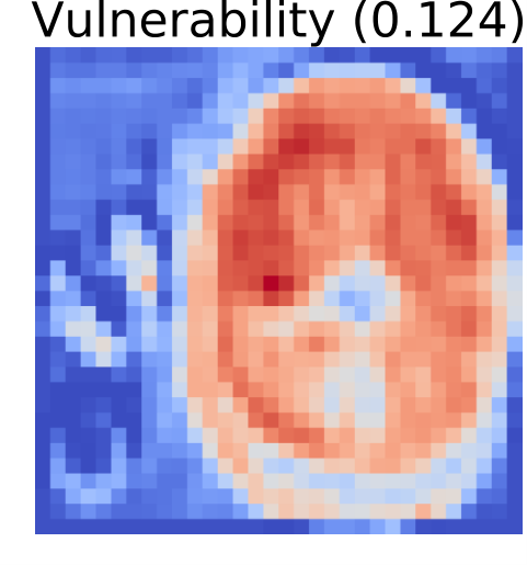
Vulnerability analysis. We next visualize the vulnerability of the latent-feature space. Figure 3 shows the vulnerability for each image for various set of datasets and the vulnerability distribution for all the features of the input layer for CIFAR-10. The results clearly show that the latent-features of the standard model are the most vulnerable, and the vulnerability decreases with the adversarial training and further suppressed by half with adversarial neural pruning. Further, the latent features of our proposed method align much better with the human perception which also results in the interpretable gradients as observed in the previous work [27, 42]. The bottom row of Figure 3 shows the histogram of the feature vulnerability defined in Equation 1 for various methods. We consistently see that standard Bayesian pruning zeros out some of the distortions, and adversarial training reduces the distortion level of all the features. On the other hand, adversarial neural pruning does both, with the largest number of features with zero distortion and low distortion level in general.

Loss landscape visualization. Figure 4 shows the loss surface of ANP compared with baseline methods. We vary the input along a linear space defined by the sign of gradient where x and y-axes represent the perturbation added in each direction and the z-axis represents the loss. The loss is highly curved in the vicinity of the data point x for the standard networks which reflects that the gradient poorly models the global landscape. On the other hand, we observe that both sparsity and adversarial training make the loss surface smooth, with our model obtaining the most smooth surface.

5 Related Work

Adversarial robustness

Since the literature on adversarial robustness of neural networks is vast, we only discuss some of the most relevant studies. Large number of defenses [43, 44, 17, 18, 45, 46] have been proposed and consequently broken by more sophisticated attack methods [22, 23, 24, 25]. One of the most successful defense is adversarial training [16], in which the neural network is trained to optimize the maximum loss obtainable using projected gradient descent over the region of allowable perturbations, which improves upon the Iterative Method [29]. However, recently, Schott et al. [47] showed that even the adversarial training [16] trained with $l_{\infty}$ can be broken with $l_{0}$-attacks. There has also been previous work which considered robust and vulnerable features at the input level. Garg et al. [48] establish a relation between adversarially robust features and the spectral property of the geometry of the dataset and Gao et al. [49] proposed to remove unnecessary features in order to get robustness. Our work is different from these existing work in that we consider and define the vulnerability at the latent feature level, which is more directly related to model prediction.

Sparsification methods

Sparsification of neural networks is becoming increasingly important with the increased deployments of deep network models to resource-limited devices. Simple heuristics-based pruning methods based on removing weights with small magnitude [50, 51, 52] have demonstrated high compression with minimal accuracy loss. However elementwise sparsity does not yield practical speed-ups and Wei et al. [53] proposed to use group sparsity to drop a neuron or a filter as a whole, that will reduce the actual network size. Recently, Bayesian and Information-theoretic approaches [54, 55, 34, 31] have shown to yield high compression rates and accuracy while providing theoretical motivation and connections to classical sparsification and regularization techniques.

Robustness and sparsity

The sparsity and robustness have been explored and modelled together in various recent works. Guo et al. [30] and Ye et al. [56] analyze sparsity and robustness from a theoretical and experimental perspective and demonstrate that appropriately higher sparsity leads to a more robust model. In contrary, Wang et al. [57] derived opposite conclusions showing that robustness decreases with increase in sparsity. However, all these works test their hypothesis on heuristic pruning techniques without adversarial training. On the contrary, we sparsify networks while explicitly targeting for robustness, as we learn the pruning (dropout) mask to minimize loss on adversarial examples.

6 Conclusion

We propose a novel adversarial neural pruning and vulnerability suppression loss, as a defense mechanism to achieve adversarial robustness as well as a means of achieving a memory and computation-efficient deep neural networks. We observe that the latent features of deep networks have a varying degree of distortion/robustness to the adversarial perturbations to the input and formally defined the vulnerability and robustness of a latent feature. This observation suggests that we can increase the robustness of the model by pruning out vulnerable latent features and by minimizing the vulnerability of the latent features, we show that sparsification thus leads to certain degree of robustness over the base network for this obvious reason. We further propose a Bayesian formulation that trains the pruning mask in an adversarial training, such that the obtained neurons are beneficial both for the accuracy of the clean and adversarial inputs. Experimental results on a range of architectures with multiple datasets demonstrate that our adversarial pruning is effective in improving the model robustness. Further qualitative analysis shows that our method obtains more interpretable latent features compared to standard counterparts, suppresses feature-level distortions in general while zeroing out perturbations at many of them, and obtains smooth loss surface.

A Adversarial beta bernoulli dropout

In this section, we prove the Equation 7 for beta bernoulli dropout. Let $\mathbf{W}$ be the parameters for the neural network and let $\mathbf{z_{n}}\in\{0,1\}^{K}$ be the mask sampled from the finite-dimensional beta-Bernoulli prior to be applied for the n-th observation $\mathbf{x_{n}}$. The generative process of the bayesian neural network can be modelled as:

$$\mathbf{W}\sim N(0,\lambda\mathbf{I}),\ \bm{\pi}\sim\prod_{k=1}^{K}beta(\pi_{k};\alpha/K,1)$$ (8)

$$\mathbf{z_{n}}|\bm{\pi}\sim\prod_{k=1}^{K}Ber(z_{n,k};\pi_{k}),\ \overset{\sim}{\mathbf{W_{n}}}=\mathbf{z_{n}}\odot\mathbf{W}$$

The goal is to compute the posterior distribution $p(\mathbf{W},\mathbf{Z},\bm{\pi}|\mathcal{D})$ and we approximate this posterior using an approximate variational distribution $q(\mathbf{W},\mathbf{Z},\bm{\pi}|\mathbf{X})$ of known parametric form. We conduct computationally efficient point-estimate for $\mathbf{W}$ to get the single value $\widehat{\mathbf{W}}$, with the weight decay regularization arising from the zero-mean Gaussian prior. For $\bm{\pi}$, we use the Kumaraswamy distribution [32] with parameters $a$ and $b$. and $\bm{z_{k}}$ is sampled by reparametrization with continuous relaxation following [31]:

$$q(\pi_{k};a_{k},b_{k})=a_{k}b_{k}\pi_{k}^{a_{k}-1}(1-\pi_{k}^{a_{k}})^{b_{k}-1}$$ (9)

$$z_{k}=sgm\left(\frac{1}{\tau}\left(\log\frac{\pi_{k}}{1-\pi_{k}}+\log\frac{u}{1-u}\right)\right)$$

where $\tau$ is a temperature continuous relaxation, $u\sim unif[0,1]$, and $sgm(x)=\frac{1}{1+e^{-x}}$. The KL-divergence between the prior and the variational distribution in closed form can then be defined as follows [58, 31]:

$$D_{KL}[q(\mathbf{Z},\bm{\pi})||p(\mathbf{Z},\bm{\pi})]=\sum_{k=1}^{K}\left\{\frac{a_{k}-\alpha/K}{a_{k}}\left(-\gamma-\Psi(b_{k})-\frac{1}{b_{k}}\right)+\log\frac{a_{k}b_{k}}{\alpha/K}-\frac{b_{k}-1}{b{k}}\right\}$$ (10)

where $\gamma$ is Euler-Mascheroni constant and $\Psi(.)$ is the digamma function. We can use Stochastic Gradient Variational Bayes (SGVB) [33] to minimize the KL divergence between the variational distribution $q(\mathbf{Z};\bm{\pi})$ of known parametric form and the true posterior $p(\mathbf{Z}|\bm{\pi})$. As we know from the SGVB framework minimizing the KL is equal to maximizing the evidence lower bound which can be done as follows:

$$\mathcal{L}=\sum_{n=1}^{N}\mathbb{E}_{q}[\log p(y_{n}|f(\mathbf{x_{n}^{adv}};\widehat{\mathbf{W}}))]-D_{KL}[q(\mathbf{Z};\bm{\pi})||p(\mathbf{Z}|\bm{\pi})]$$ (11)

where the first term measures the log-likelihood of the adversarial samples w.r.t. $q(\mathbf{Z};\bm{\pi})$ and the second term regularizes $q(\mathbf{Z};\bm{\pi})$ so it doesn’t deviate too much from the prior distribution.

B Adversarial variational information bottleneck

We further extend the idea of Adversarial Neural Pruning to variational information bottleneck. Variational information bottleneck [34] uses information theoretic bound to reduce the redundancy between adjacent layers. Consider a distribution $\mathcal{D}$ of $N$ i.i.d samples $(\mathbf{x},\mathbf{y})$ input to a neural network with $L$ layers with the network hidden layer activations as $\{\mathbf{h_{i}}\}_{i=1}^{L}$ where $\mathbf{h_{i}}\in\mathcal{R}^{r_{i}}$. Let $p(\mathbf{h_{i}}|\mathbf{h_{i-1}})$ define the conditional probability and $I(\mathbf{h_{i}};\mathbf{h_{i-1}})$ define the mutual information between $\mathbf{h_{i}}$ and $\mathbf{h_{i-1}}$ for every hidden layer in the network. For every hidden layer $\mathbf{h_{i}}$, we would like to minimize the information bottleneck [59] $I(\mathbf{h_{i};h_{i-1}})$ to remove interlayer redundancy, while simultaneously maximizing the mutual information $I(\mathbf{h_{i}};\mathbf{y})$ between $\mathbf{h_{i}}$ and the output $\mathbf{y}$ to encourage accurate predictions of adversarial examples. The layer-wise energy $\mathcal{L}_{i}$ can be written as:

$$\mathcal{L}_{i}=\gamma_{i}I(\mathbf{h_{i}};\mathbf{h_{i-1}})-I(\mathbf{h_{i}};\mathbf{y})$$ (12)

where $\gamma\geq 0$ is a coefficient that determines the strength of the bottleneck that can be defined as the degree to which we value compression over robustness.

The output layer approximates the true distribution $p(\mathbf{y}|\mathbf{h_{L}})$ via some tractable alternative $q(\mathbf{y}|\mathbf{h_{L}})$. Let $\mathbf{x^{adv}}$ be the adversarial example for $l_{\infty}$-bounded perturbations. i.e. $\triangle=\{\mathbf{x}+\delta=||\delta||_{\infty}\leq\epsilon\}$ where $\delta$ is the added perturbation from the set of allowed perturbations for each example. Using variational bounds, we can invoke the upper bound as:

$$\mathcal{L}_{i}=\gamma_{i}\mathbb{E}_{\mathbf{h_{i-1}}\sim p(\mathbf{h_{i-1})}}[KL[p(\mathbf{h_{i}}|\mathbf{h_{i-1}})||q(\mathbf{h_{i}})]]-\mathbb{E}_{\{\mathbf{x},\mathbf{y}\}\sim D,h\sim p(\mathbf{h}|\mathbf{x^{adv}})}[\log q(\mathbf{y}|\mathbf{h_{L}})]\geq\mathcal{L}_{i}$$ (13)

$\mathcal{L}_{i}$ in Equation 13 is composed of two terms, the first is the KL divergence between $p(\mathbf{h_{i}}|\mathbf{h_{i-1}})$ and $q(\mathbf{h_{i}})$, which approximates information extracted by $\mathbf{h_{i}}$ from $\mathbf{h_{i-1}}$ and the second term represents constancy with respect to the adversarial data distribution. In order to optimize Equation 13, we can define the parametric form for the distributions $p(\mathbf{h_{i}}|\mathbf{h_{i-1}})$ and $q(\mathbf{h_{i}})$ as follow:

$$\begin{split}p(\mathbf{h_{i}}|\mathbf{h_{i-1}})&=\mathcal{N}(\mathbf{h_{i}};f_{i}(\mathbf{h_{i-1}})\odot\mu_{i},diag[f_{i}(\mathbf{h_{i-1}})^{2}\odot\sigma_{i}^{2}]\\ q(\mathbf{h_{i}})&=\mathcal{N}(\mathbf{h_{i}};0,diag[\bm{\xi_{i}}])\end{split}$$ (14)

where $\bm{\xi_{i}}$ is an unknown vector of variances that can be learned from data. The gaussian assumptions help us to get an interpretable, closed-form approximation for the KL term from Equation 13, which allows us to directly optimize $\bm{\xi_{i}}$ out of the model.

$$\mathbb{E}_{\mathbf{h_{i-1}}\sim p(\mathbf{h_{i-1}})}[KL[p(\mathbf{h_{i}}|\mathbf{h_{i-1}})||q(\mathbf{h_{i}})]]=\sum_{j}\left[log\left(1+\frac{\mu_{i,j}^{2}}{\sigma_{i,j}^{2}}\right)\right]$$ (15)

The final variational information bottleneck can thus be obtained using Equation 15:

$$\mathcal{L}=\sum_{i=1}^{L}\gamma_{i}\sum_{j=1}^{r_{i}}\left[log\left(1+\frac{\mu_{i,j}^{2}}{\sigma_{i,j}^{2}}\right)\right]-\mathbb{E}_{\{\mathbf{x},\mathbf{y}\}\sim D,\mathbf{h}\sim p(\mathbf{h}|\mathbf{x^{adv}})}[\log q(\mathbf{y}|\mathbf{h_{L}})]$$ (16)

C Experiment Setup

In this section, we describe our experimental settings for all the experiments. We follow the two-step pruning procedure where we pretrain all the networks using the standard-training procedure followed by network sparsification using various sparsification methods. We train each model with 200 epochs with a fixed batch size of 64 and show the results averaged over five runs.

Our pretrained standard Lenet 5-Caffe baseline model reaches over 99.29% accuracy on MNIST and VGG-16 reaches 92.65% and 67.1% on CIFAR-10 and CIFAR-100 respectively after 200 epochs. We use Adam [60] with the learning rate for the weights to be 0.1 times smaller than those for the variational parameters as in [55, 31]. For Beta-Bernoulli Dropout, we set $\alpha/K=10^{-4}$ for all the layers and prune the neurons/filters whose expected drop probability are smaller than a fixed threshold $10^{-3}$ as originally proposed in the paper. For Beta-Bernoulli Dropout, we scaled the KL-term in Equation 11 by different values of trade-off parameter $\gamma$ where $\gamma\in\{1,4,8,10,12\}$ for Lenet-5-Caffe and $\gamma\in\{1,2,4,6,8\}$ for VGG-16. For Variational Information Bottleneck (VIBNet), we tested with trade-off parameter $\gamma$ in Equation 16 where $\gamma\in\{10,30,50,80,100\}$ for Lenet-5-Caffe with MNIST dataset and $\gamma\in\{10^{-4},1,20,40,60\}$ for VGG-16 with CIFAR-10 and CIFAR-100 dataset.

D More Experimental results

Due to the length limit of our paper, some results are illustrated here. We validate all the models with respect to three metrics for compression ratio and model complexity: i) Run-time memory footprint (Memory) - The ratio of space for storing hidden feature maps during run-time in pruned-network versus original model. ii) Floating point operations (xFLOPs) - The ratio of the number of floating point operations for original model versus pruned-network. iii) Model size (Sparsity) - The ratio of the number of zero units in original model versus compressed network. All the values are measured by computing mean and standard deviation across 3 trials upon randomly chosen seeds, respectively. We also report the clean accuracy, vulnerability metric (Equation 2) and accuracy on adversarial examples generated from $l_{\infty}$ white box and black box attack [38].

Table Appendix-1 also shows the results of Adversarial Neural Pruning with Variational Information Bottleneck. We can observe that both ANP (BBD) and ANP (VIB) outperform the base adversarial training for robustness of adversarial examples while also achieving memory and computation efficiency. We emphasize that ANP can similarly be extended to any existing or future sparsification method to improve performance.

Table Appendix-2 shows the number of units for all the baselines and our proposed method. Figure D.2 shows the histogram of the feature vulnerability for various datasets. We can consistently observe that standard Bayesian pruning zeros out some of the distortions, adversarial training reduces the distortion level of all the features and adversarial neural pruning does both, with the largest number of features with zero distortion and low distortion level in general which confirms that our adversarial neural pruning works successfully as a defense against adversarial attacks.

Table Appendix-1: Comparison of different methods for MNIST on Lenet-5-Caffe, CIFAR-10 and CIFAR-100 on VGG-16 architectures. We report compression in terms of Floating Point Operations (FLOPs), memory and sparsity, robustness in terms of accuracy (average and stddev) and vulnerability on adversarial examples generated from white-box and black-box attack.

						Adversarial accuracy (%)		Vulnerability
	Model	Clean acc.(%)	xFLOPs	Memory (%)	Sparsity (%)	White box	Black box	White box	Black box
MNIST	Standard	99.29	1.0	100.0	0.00	0.00	8.02	0.129	0.113
	BP (BBD)	99.34	4.14	9.68	83.48	0.00	12.99	0.091	0.078
	BP (VIB)	99.32	4.34	9.39	82.46	5.66	15.47	0.074	1.265
	AT	99.14	1.0	100.0	0.00	88.03	94.18	0.045	0.040
	AT BNN	99.16	0.5	200.0	0.00	88.44	94.87	0.045	0.023
	Pretrained AT	99.18	1.0	100.0	0.00	88.26	94.49	0.043	0.038
	AT-VS (ours)	98.98	1.0	100.0	0.00	89.50	95.16	0.022	0.020
	ANP (BBD) (ours)	98.67	9.77	6.69	84.45	89.12	94.83	0.020	0.019
	ANP (VIB) (ours)	98.86	4.87	10.06	78.48	89.01	94.94	0.017	0.015
	AT-VS (BBD) (ours)	99.05	7.30	8.59	78.91	89.89	95.24	0.014	0.013
CIFAR-10	Standard	92.65	1.0	100.0	0.00	12.02	40.89	0.078	0.066
	BP (BBD)	93.00	2.36	12.39	75.82	13.36	39.14	0.037	0.033
	BP (VIB)	92.73	2.38	12.28	76.35	12.35	41.32	0.035	0.032
	AT	87.37	1.0	100.0	0.00	48.93	63.61	0.051	0.047
	AT BNN	86.54	0.5	200.0	0.00	51.59	64.20	0.044	0.038
	Pretrained AT	87.50	1.0	100.0	0.00	52.25	66.10	0.041	0.036
	AT-VS (ours)	87.89	1.0	100.0	0.00	51.52	66.60	0.024	0.023
	ANP (BBD) (ours)	88.74	2.33	12.46	76.39	55.31	70.30	0.022	0.020
	ANP (VIB) (ours)	87.41	2.37	12.15	76.50	52.13	67.95	0.025	0.024
	ANP-VS (BBD) (ours)	88.95	2.43	12.09	77.02	56.16	70.70	0.017	0.016
CIFAR-100	Standard	67.10	1.0	100.0	0.00	2.95	15.90	0.135	0.111
	BP (BBD)	69.08	1.93	18.87	63.05	3.54	17.07	0.066	0.057
	BP (VIB)	69.09	1.95	18.46	63.84	2.73	19.53	0.084	0.073
	AT	56.43	1.0	100.0	0.00	18.34	33.39	0.077	0.072
	AT BNN	53.21	0.5	200.0	0.00	19.40	30.38	0.078	0.071
	Pretrained AT	57.14	1.0	100.0	0.00	19.86	35.42	0.071	0.065
	AT-VS (ours)	57.14	1.0	100.0	0.00	19.22	33.91	0.072	0.039
	ANP (BBD) (ours)	57.80	2.00	16.87	66.63	21.29	36.27	0.037	0.032
	ANP (VIB) (ours)	59.77	2.02	17.55	64.75	20.43	36.31	0.051	0.047
	ANP-VS (BBD) (ours)	57.38	2.06	16.46	67.19	21.92	37.84	0.035	0.030

Figure D.1: Visualization of convolutional features of first layer of adversarial trained VGG-16 network with CIFAR-100 dataset. b) - d) represents the vulnerable latent-feature with high vulnerability (vulnerable feature) on b) clean example, c) Adversarial example d) Vulnerability (difference between clean and adversarial example) e) - f) represents the vulnerable latent-feature with low vulnerability (robust feature) on e) clean example, f) Adversarial example g) Vulnerability (difference between clean and adversarial example)

Figure D.2: Histogram of vulnerability of the features for the input layer for MNIST in the top row, CIFAR-10 in the middle and CIFAR-100 in the bottom with the number of zeros shown in orange color.

Table Appendix-2: Clean and adversarial accuracy for models trained with and without adversarial training with flops, memory and sparsity percentage reduction.

	Model	No of neurons
MNIST	Standard	20 – 50 – 800 – 500
	BP (BBD)	14 – 21 – 150 – 49
	BP (VIB)	12 – 19 – 160 – 37
	AT	20 – 50 – 800 – 500
	ANP (BBD)	7 –  21 – 147 – 46
	ANP (VIB)	10 – 23 – 200 – 53
CIFAR-10	Standard	64 – 64 – 128 – 128 – 256 – 256 – 256 – 512 – 512 – 512 – 512 – 512 – 512 – 512 – 512
	BP (BBD)	57 – 59 – 127 – 101 – 150 – 71 –   31 –  41 –   35 –   10 –   46 –   48 –  16 –  16 –  25
	BP (VIB)	49 – 56 – 106 – 92 –  157 – 74 –   26 –  43 –   32 –   10 –   39 –   40 –  7 –   7 –   13
	AT	64 – 64 – 128 – 128 – 256 – 256 – 256 – 512 – 512 – 512 – 512 – 512 – 512 – 512 – 512
	ANP (BBD)	42 – 57 – 113 – 96 –  147 –  68 –  25 –  37 –  27 –   9 –   39 –   40 –   13 –   13 –   12
	ANP (VIB)	40 – 57 – 104 – 93 –  174 –  96 –  30 –  48 –  39 –   9 –   49 –   57 –   10 –   10 –   12
CIFAR-100	Baseline	64 – 64 – 128 – 128 – 256 – 256 – 256 – 512 – 512 – 512 – 512 – 512 – 512 – 512 – 512
	BBD	62 – 64 – 128 – 123 – 244 – 203 – 84 –  130 –   95 –   18 –  152 –  157 –  32 –  32 –  101
	VIB	52 – 64 – 119 – 116 –  229 – 179 – 83 –  99 –  71 –  17 –   107 –  110 –  12 –  11 –  49
	Adv. Train	64 – 64 – 128 – 128 – 256 – 256 – 256 – 512 – 512 – 512 – 512 – 512 – 512 – 512 – 512
	Adv. BBD	60 – 64 – 126 – 122 –  235 – 185 – 77 –  128 –  101 –  17 –  165 –  177 –  35 –  35 –  45
	Adv. VIB	44 – 58 – 110 – 109 –  207 – 155 – 81 –  86 –   66 –   19 –   88 –   86 –   15 –  15 –  36

E Features Visualization

One might also be curious about the representation of the robust and vulnerable features in the latent-feature space. In this section, we visualize the robust and vulnerable features in terms of the definitions of robust and vulnerable features in the latent-feature space from our paper. Figure D.1 shows the visualization of robust and vulnerable features in the latent space for adversarial training. It is important to observe that adversarial training also contains features with high vulnerability (vulnerable feature) and features with less vulnerability (robust feature) which align with our observation that the latent features have a varying degree of susceptibility to adversarial perturbations to the input. As future work, we plan to explore more effective ways to suppress perturbation at the intermediate latent features of deep networks.

References

- [1] Alex Krizhevsky, Ilya Sutskever, and Geoffrey E Hinton. Imagenet classification with deep convolutional neural networks. In F. Pereira, C. J. C. Burges, L. Bottou, and K. Q. Weinberger, editors, Advances in Neural Information Processing Systems 25, pages 1097–1105. Curran Associates, Inc., 2012.
- [2] Kaiming He, Xiangyu Zhang, Shaoqing Ren, and Jian Sun. Delving deep into rectifiers: Surpassing human-level performance on imagenet classification. CoRR, abs/1502.01852, 2015.
- [3] Jiankang Deng, Jia Guo, and Stefanos Zafeiriou. Arcface: Additive angular margin loss for deep face recognition. CoRR, abs/1801.07698, 2018.
- [4] Vijay Badrinarayanan, Alex Kendall, and Roberto Cipolla. Segnet: A deep convolutional encoder-decoder architecture for image segmentation. IEEE Transactions on Pattern Analysis and Machine Intelligence, 39:2481–2495, 2015.
- [5] Kaiming He, Georgia Gkioxari, Piotr Dollár, and Ross B. Girshick. Mask r-cnn. 2017 IEEE International Conference on Computer Vision (ICCV), pages 2980–2988, 2017.
- [6] David Silver, Aja Huang, Christopher Maddison, Arthur Guez, Laurent Sifre, George Driessche, Julian Schrittwieser, Ioannis Antonoglou, Veda Panneershelvam, Marc Lanctot, Sander Dieleman, Dominik Grewe, John Nham, Nal Kalchbrenner, Ilya Sutskever, Timothy Lillicrap, Madeleine Leach, Koray Kavukcuoglu, Thore Graepel, and Demis Hassabis. Mastering the game of go with deep neural networks and tree search. Nature, 529:484–489, 01 2016.
- [7] David Silver, Julian Schrittwieser, Karen Simonyan, Ioannis Antonoglou, Aja Huang, Arthur Guez, Thomas Hubert, Lucas Baker, Matthew Lai, Adrian Bolton, Yutian Chen, Timothy Lillicrap, Fan Hui, Laurent Sifre, George Driessche, Thore Graepel, and Demis Hassabis. Mastering the game of go without human knowledge. Nature, 550:354–359, 10 2017.
- [8] Andre Esteva, Brett Kuprel, Roberto A Novoa, Justin Ko, Susan M Swetter, Helen M Blau, and Sebastian Thrun. Dermatologist-level classification of skin cancer with deep neural networks. Nature, 542(7639):115, 2017.
- [9] Pranav Rajpurkar, Jeremy Irvin, Kaylie Zhu, Brandon Yang, Hershel Mehta, Tony Duan, Daisy Yi Ding, Aarti Bagul, Curtis P. Langlotz, Katie S. Shpanskaya, Matthew P. Lungren, and Andrew Y. Ng. Chexnet: Radiologist-level pneumonia detection on chest x-rays with deep learning. ArXiv, abs/1711.05225, 2017.
- [10] Mariusz Bojarski, Davide Del Testa, Daniel Dworakowski, Bernhard Firner, Beat Flepp, Prasoon Goyal, Lawrence D. Jackel, Mathew Monfort, Urs Muller, Jiakai Zhang, Xin Zhang, Jake Zhao, and Karol Zieba. End to end learning for self-driving cars. CoRR, abs/1604.07316, 2016.
- [11] Li Erran Li, Eric Chen, Jeremy Hermann, Pusheng Zhang, and Luming Wang. Scaling machine learning as a service. In Claire Hardgrove, Louis Dorard, Keiran Thompson, and Florian Douetteau, editors, Proceedings of The 3rd International Conference on Predictive Applications and APIs, volume 67 of Proceedings of Machine Learning Research, pages 14–29, Microsoft NERD, Boston, USA, 11–12 Oct 2017. PMLR.
- [12] Christian Szegedy, Wojciech Zaremba, Ilya Sutskever, Joan Bruna, Dumitru Erhan, Ian J. Goodfellow, and Rob Fergus. Intriguing properties of neural networks. CoRR, abs/1312.6199, 2013.
- [13] Ian J. Goodfellow, Jonathon Shlens, and Christian Szegedy. Explaining and Harnessing Adversarial Examples. arXiv e-prints, page arXiv:1412.6572, Dec 2014.
- [14] Nicolas Papernot, Patrick D. McDaniel, Xi Wu, Somesh Jha, and Ananthram Swami. Distillation as a defense to adversarial perturbations against deep neural networks. 2016 IEEE Symposium on Security and Privacy (SP), pages 582–597, 2015.
- [15] Weilin Xu, David Evans, and Yanjun Qi. Feature squeezing: Detecting adversarial examples in deep neural networks. CoRR, abs/1704.01155, 2017.
- [16] Aleksander Madry, Aleksandar Makelov, Ludwig Schmidt, Dimitris Tsipras, and Adrian Vladu. Towards deep learning models resistant to adversarial attacks. In International Conference on Learning Representations, 2018.
- [17] Jacob Buckman, Aurko Roy, Colin Raffel, and Ian Goodfellow. Thermometer encoding: One hot way to resist adversarial examples. In International Conference on Learning Representations, 2018.
- [18] Guneet S. Dhillon, Kamyar Azizzadenesheli, Jeremy D. Bernstein, Jean Kossaifi, Aran Khanna, Zachary C. Lipton, and Animashree Anandkumar. Stochastic activation pruning for robust adversarial defense. In International Conference on Learning Representations, 2018.
- [19] Cihang Xie, Jianyu Wang, Zhishuai Zhang, Zhou Ren, and Alan Yuille. Mitigating adversarial effects through randomization. In International Conference on Learning Representations, 2018.
- [20] Florian Tramèr, Alexey Kurakin, Nicolas Papernot, Ian Goodfellow, Dan Boneh, and Patrick McDaniel. Ensemble adversarial training: Attacks and defenses. In International Conference on Learning Representations, 2018.
- [21] Xuanqing Liu, Yao Li, Chongruo Wu, and Cho-Jui Hsieh. Adv-BNN: Improved adversarial defense through robust bayesian neural network. In International Conference on Learning Representations, 2019.
- [22] Nicholas Carlini and David A. Wagner. Towards evaluating the robustness of neural networks. CoRR, abs/1608.04644, 2016.
- [23] Anish Athalye, Nicholas Carlini, and David A. Wagner. Obfuscated gradients give a false sense of security: Circumventing defenses to adversarial examples. CoRR, abs/1802.00420, 2018.
- [24] Jonathan Uesato, Brendan O’Donoghue, Aäron van den Oord, and Pushmeet Kohli. Adversarial risk and the dangers of evaluating against weak attacks. CoRR, abs/1802.05666, 2018.
- [25] Anish Athalye and Nicholas Carlini. On the robustness of the CVPR 2018 white-box adversarial example defenses. CoRR, abs/1804.03286, 2018.
- [26] Ludwig Schmidt, Shibani Santurkar, Dimitris Tsipras, Kunal Talwar, and Aleksander Madry. Adversarially robust generalization requires more data. In S. Bengio, H. Wallach, H. Larochelle, K. Grauman, N. Cesa-Bianchi, and R. Garnett, editors, Advances in Neural Information Processing Systems 31, pages 5014–5026. Curran Associates, Inc., 2018.
- [27] Dimitris Tsipras, Shibani Santurkar, Logan Engstrom, Alexander Turner, and Aleksander Madry. Robustness may be at odds with accuracy. In International Conference on Learning Representations, 2019.
- [28] Hongyang Zhang, Yaodong Yu, Jiantao Jiao, Eric Xing, Laurent El Ghaoui, and Michael Jordan. Theoretically principled trade-off between robustness and accuracy. In International Conference on Machine Learning, pages 7472–7482, 2019.
- [29] Alexey Kurakin, Ian J. Goodfellow, and Samy Bengio. Adversarial machine learning at scale. CoRR, abs/1611.01236, 2016.
- [30] Yiwen Guo, Chao Zhang, Changshui Zhang, and Yurong Chen. Sparse dnns with improved adversarial robustness. CoRR, abs/1810.09619, 2018.
- [31] Juho Lee, Saehoon Kim, Jaehong Yoon, Hae Beom Lee, Eunho Yang, and Sung Ju Hwang. ADAPTIVE NETWORK SPARSIFICATION VIA DEPENDENT VARIATIONAL BETA-BERNOULLI DROPOUT, 2019.
- [32] P. Kumaraswamy. A generalized probability density function for double-bounded random processes. Journal of Hydrology, 46(1):79–88, 1980.
- [33] Durk P Kingma, Tim Salimans, and Max Welling. Variational dropout and the local reparameterization trick. In C. Cortes, N. D. Lawrence, D. D. Lee, M. Sugiyama, and R. Garnett, editors, Advances in Neural Information Processing Systems 28, pages 2575–2583. Curran Associates, Inc., 2015.
- [34] Bin Dai, Chen Zhu, and David P. Wipf. Compressing neural networks using the variational information bottleneck. CoRR, abs/1802.10399, 2018.
- [35] Yann LeCun. The mnist database of handwritten digits. http://yann. lecun. com/exdb/mnist/, 1998.
- [36] Alex Krizhevsky. Learning multiple layers of features from tiny images. University of Toronto, 05 2012.
- [37] Karen Simonyan and Andrew Zisserman. Very deep convolutional networks for large-scale image recognition. CoRR, abs/1409.1556, 2015.
- [38] Nicolas Papernot, Patrick D. McDaniel, Ian J. Goodfellow, Somesh Jha, Z. Berkay Celik, and Ananthram Swami. Practical black-box attacks against deep learning systems using adversarial examples. CoRR, abs/1602.02697, 2016.
- [39] Martín Abadi, Paul Barham, Jianmin Chen, Zhifeng Chen, Andy Davis, Jeffrey Dean, Matthieu Devin, Sanjay Ghemawat, Geoffrey Irving, Michael Isard, et al. Tensorflow: A system for large-scale machine learning. In 12th USENIX Symposium on Operating Systems Design and Implementation (OSDI 16), pages 265–283, 2016.
- [40] Logan Engstrom, Andrew Ilyas, and Anish Athalye. Evaluating and understanding the robustness of adversarial logit pairing. arXiv preprint arXiv:1807.10272, 2018.
- [41] Dan Hendrycks, Kimin Lee, and Mantas Mazeika. Using pre-training can improve model robustness and uncertainty. In International Conference on Machine Learning, pages 2712–2721, 2019.
- [42] Beomsu Kim, Junghoon Seo, and Taegyun Jeon. Bridging adversarial robustness and gradient interpretability. CoRR, abs/1903.11626, 2019.
- [43] Nicolas Papernot, Patrick D. McDaniel, Xi Wu, Somesh Jha, and Ananthram Swami. Distillation as a defense to adversarial perturbations against deep neural networks. CoRR, abs/1511.04508, 2015.
- [44] Weilin Xu, David Evans, and Yanjun Qi. Feature squeezing: Detecting adversarial examples in deep neural networks. CoRR, abs/1704.01155, 2017.
- [45] Yang Song, Taesup Kim, Sebastian Nowozin, Stefano Ermon, and Nate Kushman. Pixeldefend: Leveraging generative models to understand and defend against adversarial examples. In International Conference on Learning Representations, 2018.
- [46] Eric Wong and J. Zico Kolter. Provable defenses against adversarial examples via the convex outer adversarial polytope. In ICML, 2018.
- [47] Lukas Schott, Jonas Rauber, Matthias Bethge, and Wieland Brendel. Towards the first adversarially robust neural network model on MNIST. In International Conference on Learning Representations, 2019.
- [48] Shivam Garg, Vatsal Sharan, Brian Zhang, and Gregory Valiant. A spectral view of adversarially robust features. In S. Bengio, H. Wallach, H. Larochelle, K. Grauman, N. Cesa-Bianchi, and R. Garnett, editors, Advances in Neural Information Processing Systems 31, pages 10138–10148. Curran Associates, Inc., 2018.
- [49] Ji Gao, Beilun Wang, and Yanjun Qi. Deepmask: Masking DNN models for robustness against adversarial samples. CoRR, abs/1702.06763, 2017.
- [50] Nikko Ström. Sparse connection and pruning in large dynamic artificial neural networks, 1997.
- [51] Maxwell D. Collins and Pushmeet Kohli. Memory bounded deep convolutional networks. CoRR, abs/1412.1442, 2014.
- [52] Song Han, Jeff Pool, John Tran, and William J. Dally. Learning both weights and connections for efficient neural networks. In NIPS, 2015.
- [53] Wei Wen, Chunpeng Wu, Yandan Wang, Yiran Chen, and Hai Li. Learning structured sparsity in deep neural networks. In D. D. Lee, M. Sugiyama, U. V. Luxburg, I. Guyon, and R. Garnett, editors, Advances in Neural Information Processing Systems 29, pages 2074–2082. Curran Associates, Inc., 2016.
- [54] Dmitry Molchanov, Arsenii Ashukha, and Dmitry Vetrov. Variational dropout sparsifies deep neural networks. In Proceedings of the 34th International Conference on Machine Learning - Volume 70, ICML’17, pages 2498–2507. JMLR.org, 2017.
- [55] Kirill Neklyudov, Dmitry Molchanov, Arsenii Ashukha, and Dmitry P. Vetrov. Structured bayesian pruning via log-normal multiplicative noise. In NIPS, 2017.
- [56] Shaokai Ye, Siyue Wang, Xiao Wang, Bo Yuan, Wujie Wen, and Xue Lin. Defending dnn adversarial attacks with pruning and logits augmentation, 2018.
- [57] Luyu Wang, Gavin Weiguang Ding, Ruitong Huang, Yanshuai Cao, and Yik Chau Lui. Adversarial robustness of pruned neural networks, 2018.
- [58] Eric Nalisnick and Padhraic Smyth. Stick-breaking variational autoencoders. arXiv preprint arXiv:1605.06197, 2016.
- [59] Naftali Tishby, Fernando C Pereira, and William Bialek. The information bottleneck method. arXiv preprint physics/0004057, 2000.
- [60] Diederik P. Kingma and Jimmy Ba. Adam: A method for stochastic optimization. CoRR, abs/1412.6980, 2015.