Proximally Constrained Methods for Weakly Convex Optimization with Weakly Convex Constraints

Abstract

Optimization models with non-convex constraints arise in many tasks in machine learning, e.g., learning with fairness constraints or Neyman-Pearson classification with non-convex loss. Although many efficient methods have been developed with theoretical convergence guarantees for non-convex unconstrained problems, it remains a challenge to design provably efficient algorithms for problems with non-convex functional constraints. This paper proposes a class of subgradient methods for constrained optimization where the objective function and the constraint functions are are weakly convex. Our methods solve a sequence of strongly convex subproblems, where a proximal term is added to both the objective function and each constraint function. Each subproblem can be solved by various algorithms for strongly convex optimization. Under a uniform Slater’s condition, we establish the computation complexities of our methods for finding a nearly stationary point.

1 Introduction

Continuous optimization models with nonlinear constraints have been widely used in many disciplines including machine learning, statistics, and data mining with many real-world applications. A general optimization problem with inequality constraints is formulated as

$$f^{*}\equiv\min_{{\mathbf{x}}\in\mathcal{X}}\{f({\mathbf{x}})\equiv f_{0}({\mathbf{x}})\}\quad\text{s.t.}\quad g({\mathbf{x}})\equiv\max_{i=1,\dots,m}f_{i}({\mathbf{x}})\leq 0,~i=1,2,\dots,m.$$ (1)

Here, we assume that $\mathcal{X}\subset\mathbb{R}^{d}$ is a compact convex set that allows for a simple projection and $f_{i}$ for $i=0,\dots,m$ are weakly-convex (potentially non-smooth) functions. A solution $\bar{\mathbf{x}}\in\mathcal{X}$ is $\varepsilon$-optimal if $f(\bar{\mathbf{x}})-f^{*}\leq\varepsilon$ and $\varepsilon$-feasible if $\bar{\mathbf{x}}\in\mathcal{X}$ and $g(\bar{\mathbf{x}})\leq\varepsilon$. Many optimization models in machine learning contain nonlinear constraints. Examples include Neyman-Pearson classification [38] and learning with dataset constraints [21] (e.g. fairness constraints and churn rate constraints).

Optimization problems with a convex objective function and convex constraints have been well studied in literature with many efficient algorithms and their theoretical complexity developed [5, 4, 32]. However, the parallel development for optimization with non-convex objective functions and non-convex constraints, especially for theoretically provable algorithms, remains limited, restricting the practices of statistical modeling and decision making in many disciplines. It is well-known that finding a global minimizer for a general non-convex function without any constraints has been intractable [42]. The difficulty will increase when constraints appear and will increase even further when those constraints are non-convex.

Therefore, when designing an algorithm for (1) with non-convex objective and constraint functions, the first question to be addressed is what kind of solutions can the algorithm guarantees and what complexity the algorithm has in order to find such solutions. In the recent studies on unconstrained or simply constrained non-convex minimization [13, 14, 12, 15, 16, 17, 19, 20, 24, 33, 36, 37], algorithms have been proposed to find a nearly stationary point, which is a feasible solution close to another feasible solution where the subdifferential of the objective function almost contains zero. However, these methods and analysis cannot be applied to (1) as they require the exact projection to the feasible set which is hard to perform for (1) due to the functional constraints. To address this issue, in this work, we propose a class of first-order methods for (1) where the objective function and the constraint functions are all weakly convex. Our methods solve a sequence of strongly convex subproblems of a proximal-point type where, different from the traditional proximal-point method, a proximal term is also added to each constraint function instead of just the objective function. Each subproblem can be solved by an algorithm for strongly convex optimization. Under a uniform Slater’s condition, we establish the complexities of our methods for finding a nearly stationary point. We will discuss some applications of (1) in machine learning next.

1.1 Optimization Problems in Machine Learning with Nonlinearly Constraints

Multi-class Neyman-Pearson Classification: In multi-class classification, there exist $K$ classes of data, denoted by $\xi_{k}$ for $k=1,2,\dots,K$, each of which has its own distribution. To classify each data into one of the $K$ classes, one can rely on $K$ linear models ${\mathbf{x}}_{k}$, $k=1,2,\dots,K$ and predict the class of a data point $\xi$ as $\mathop{\mathrm{arg\,max}{}}_{k=1,2,\dots,K}{\mathbf{x}}_{k}^{\top}\xi$. To achieve a high classification accuracy, we would like the value ${\mathbf{x}}_{k}^{\top}\xi_{k}-{\mathbf{x}}_{l}^{\top}\xi_{k}$ with $k\neq l$ to be positively large [46, 11], which can be achieved by minimizing the expected loss $\mathbb{E}\phi({\mathbf{x}}_{k}^{\top}\xi_{k}-{\mathbf{x}}_{l}^{\top}\xi_{k})$, where $\phi$ is a non-increasing potentially non-convex loss function and $\mathbb{E}$ is the expectation taken over $\xi_{k}$. When training these $K$ linear models, one can prioritize minimizing the loss on class $1$ while control the losses on other classes by solving

$$\min_{\|{\mathbf{x}}_{k}\|_{2}\leq\lambda,k=1,\dots,K}\sum_{l\neq 1}\mathbb{E}[\phi({\mathbf{x}}_{1}^{\top}\xi_{1}-{\mathbf{x}}_{l}^{\top}\xi_{1})],~\text{s.t.}~\sum_{l\neq k}\mathbb{E}[\phi({\mathbf{x}}_{k}^{\top}\xi_{k}-{\mathbf{x}}_{l}^{\top}\xi_{k})]\leq r_{k}\quad k=2,3,\dots,K,$$

where $r_{k}$ controls the loss for class $k$ and $\lambda$ is a regularization parameter. When $\xi$ follows the empirical distribution over a finite dataset, the expectations above are essentially sample averages so that this problem becomes a deterministic optimization problem.

Learning Data-Driven Constraints: Problem (1) also covers many machine learning models with data-driven constraints [21]. The examples include the constraints that impose conditions on the coverage rates, churn rates, or fairness of a predictive model. More details can be found in [21]. Here, we focus on learning a classifier with parity-based fairness constraints [21, 56, 55]. Suppose $({\mathbf{a}},b)$ is a point from a distribution $\mathcal{D}$ where $b\in\{1,-1\}$ is the label. Let $\mathcal{D}_{M}$ and $\mathcal{D}_{F}$ be two different distributions of points (not necessarily labeled), e.g., $\mathcal{D}_{M}$ and $\mathcal{D}_{F}$ may represent the male and female groups. The training of a classifier with fairness constraints can be formulated as

$$\min_{\|{\mathbf{x}}\|_{2}\leq\lambda}\mathbb{E}_{({\mathbf{a}},b)\sim\mathcal{D}}[\phi(-b{\mathbf{a}}^{\top}{\mathbf{x}})]$$

$$\quad\text{s.t.}\mathbb{E}_{{\mathbf{a}}\sim\mathcal{D}_{M}}[\sigma({\mathbf{a}}^{\top}{\mathbf{x}})]+\beta\mathbb{E}_{{\mathbf{a}}\sim\mathcal{D}_{F}}[\sigma(-{\mathbf{a}}^{\top}{\mathbf{x}})]\leq r,~\mathbb{E}_{{\mathbf{a}}\sim\mathcal{D}_{F}}[\sigma({\mathbf{a}}^{\top}{\mathbf{x}})]+\beta\mathbb{E}_{{\mathbf{a}}\sim\mathcal{D}_{M}}[\sigma(-{\mathbf{a}}^{\top}{\mathbf{x}})]\leq r$$

where $\phi$ is a non-increasing potentially non-convex loss function, $\sigma=\frac{\exp(z)}{1+\exp(z)}$, $\lambda$ is a regularization parameter, $\beta$ is a positive balance parameter and $r$ is a constraint parameter. The objective function is the training loss of ${\mathbf{x}}$. The terms $\sigma({\mathbf{a}}^{\top}{\mathbf{x}})$ and $\sigma(-{\mathbf{a}}^{\top}{\mathbf{x}})$ represent the predicted probabilities of ${\mathbf{a}}$ being in the positive and the negative class, respectively. The left hand side of the first constraint will be large if the model ${\mathbf{x}}$ is very “unfair” in the sense that it makes ${\mathbf{a}}^{\top}{\mathbf{x}}$ very negative for most of ${\mathbf{a}}$ from $\mathcal{D}_{M}$ but very positive for most of ${\mathbf{a}}$ from $\mathcal{D}_{F}$. The second constraint can be interpreted similarly. Choosing appropriate $r$ forces the left hand sides of both constraints low so that the obtained model will be fair to both $\mathcal{D}_{M}$ and $\mathcal{D}_{F}$. Another example of fairness constraint is given in Section 5.

1.2 Contributions

We summarize our contributions as follows.

• We propose a class of algorithms (Algorithm 1) for (1) when all $f_{i}$ are weakly convex. This method approximately solves a proximally guided strongly convex subproblem (9) in each main iteration with precision $O(\epsilon^{2})$ using a suitable first-order method. We show that our method finds a nearly $\epsilon$-stationary point (Definition 1) for (1) in $O(\frac{1}{\epsilon^{2}})$ main iterations.

• When each $f_{i}$ is a deterministic function, we develop a new variant of the switching subgradient method [34] to solve (9). We show that the complexity of Algorithm 1 for finding a nearly $\epsilon$-stationary point is $O(\frac{1}{\epsilon^{4}})$.

• When each $f_{i}$ is given as an expectation of a stochastic function, we directly use the stochastic subgradient method by [53] to solve (9). We show that the complexity of Algorithm 1 for finding a nearly $\epsilon$-stationary point is $\tilde{O}(\frac{1}{\epsilon^{6}})$.

2 Related Work

There has been growing interest in first-order algorithms for non-convex minimization problems with no constraints or simple constraints in both stochastic and deterministic setting. Initially, the research in this direction mainly focus on the problem with a smooth objective function [19, 51, 20, 37, 36, 24, 1, 2, 22]. Recently, more studies have been developed on the algorithms and theories for non-convex minimization problems with non-smooth objective functions after assuming the objective function is weakly convex [14, 13, 17, 15, 9, 58]. These works tackle the non-smoothness of objective function by introducing the Moreau envelope of objective function and analyze the complexity of finding a nearly stationary point. However, these methods are not directly applicable to (1) because of the functional constraints.

The studies on convex optimization with functional constraints have a long history [5, 4, 32, 41, and references therein]. The recent development in the first-order methods for convex optimization with convex constraints include [30, 57, 8, 52, 45, 49, 48, 47, 53, 28, 27, 3, 18] for deterministic constraints and [25, 54] for stochastic constraints. [44] propose a primal-dual Frank-Wolfe method for (1) with non-convex $f_{0}$ but linear $f_{i}$ for $i=1,2,\dots,m$. Different from these works, this paper study the problems where the objective function and the constaints are all non-convex.

An exact penalty method has been developed by [6] to solve non-convex optimization problems with non-convex constraints. Each subproblem in the exact penalty method was solved by either a first-order trust-region method or a quadratic regularization method. Their methods have been extended by [43] to handle stochastic objective function and by [7] to remove the boundness assumption on the penalty parameters and obtain a lower complexity. However, these works assume the objective and constraint functions are all smooth while our results can be applied to non-smooth problems.

3 Preliminaries

Let $\|\cdot\|$ be the $\ell_{2}$-norm. For $h:\mathbb{R}^{d}\rightarrow\mathbb{R}\cup\{+\infty\}$, the subdifferential of $h$ at ${\mathbf{x}}$ is

$$\partial h({\mathbf{x}})=\big\{\bm{\zeta}\in\mathbb{R}^{d}\big|h({\mathbf{x}}^{\prime})\geq h({\mathbf{x}})+\bm{\zeta}^{\top}({\mathbf{x}}^{\prime}-{\mathbf{x}})+o(\|{\mathbf{x}}^{\prime}-{\mathbf{x}}\|),~{\mathbf{x}}^{\prime}\rightarrow{\mathbf{x}}\big\},$$

where $\bm{\zeta}\in\partial h({\mathbf{x}})$ is a subgradient of $h$ at ${\mathbf{x}}$. We say $h$ is $\mu$-strongly convex ($\mu\geq 0$) on $\mathcal{X}$ if

$$h({\mathbf{x}})\geq h({\mathbf{x}}^{\prime})+\bm{\zeta}^{\top}({\mathbf{x}}-{\mathbf{x}}^{\prime})+\frac{\mu}{2}\|{\mathbf{x}}-{\mathbf{x}}^{\prime}\|^{2}$$

for any $({\mathbf{x}},{\mathbf{x}}^{\prime})\in\mathcal{X}\times\mathcal{X}$ and any $\bm{\zeta}\in\partial h({\mathbf{x}}^{\prime})$. We say $h$ is $\rho$-weakly convex ($\rho\geq 0$) on $\mathcal{X}$ if

$$h({\mathbf{x}})\geq h({\mathbf{x}}^{\prime})+\bm{\zeta}^{\top}({\mathbf{x}}-{\mathbf{x}}^{\prime})-\frac{\rho}{2}\|{\mathbf{x}}-{\mathbf{x}}^{\prime}\|_{2}^{2}$$

for any $({\mathbf{x}},{\mathbf{x}}^{\prime})\in\mathcal{X}\times\mathcal{X}$ and any $\bm{\zeta}\in\partial h({\mathbf{x}}^{\prime})$. We denote the normal cone of $\mathcal{X}$ at ${\mathbf{x}}$ by $\mathcal{N}_{\mathcal{X}}({\mathbf{x}})$ and the distance from ${\mathbf{x}}$ to a set $S$ by $\text{Dist}({\mathbf{x}},S)=\min_{{\mathbf{y}}\in S}\|{\mathbf{x}}-{\mathbf{y}}\|$.

The following assumptions about (1) are made throughout the paper:

Assumption 1.

The following statements hold:

• $f_{i}({\mathbf{x}})$ is closed and $\rho$-weakly convex with $\partial f_{i}({\mathbf{x}})\neq\emptyset$ on any ${\mathbf{x}}\in\mathcal{X}$ for $i=0,1,\dots,m$.

• $\min\limits_{{\mathbf{y}}\in\mathcal{X}}\{g({\mathbf{y}})+\frac{\rho+\rho_{\epsilon}}{2}\|{\mathbf{y}}-{\mathbf{x}}\|^{2}\}<-\sigma_{\epsilon}$ for any $\epsilon^{2}$-feasible solution ${\mathbf{x}}$ (${\mathbf{x}}\in\mathcal{X}$ and $g({\mathbf{x}})\leq\epsilon^{2}$) for some positive constants $\sigma_{\epsilon}$ and $\rho_{\epsilon}$. We call this condition uniform Slater’s condition.

• The domain $\mathcal{X}$ is compact such that $\max_{{\mathbf{x}},{\mathbf{x}}^{\prime}\in\mathcal{X}}\|{\mathbf{x}}-{\mathbf{x}}^{\prime}\|\leq D$ for some constant $D$.

• $f_{\text{lb}}\equiv\min_{{\mathbf{x}}\in\mathcal{X}}f({\mathbf{x}})>-\infty$.

• We have access to an initial $\epsilon^{2}$-feasible solution ${\mathbf{x}}_{\text{feas}}$ with ${\mathbf{x}}_{\text{feas}}\in\mathcal{X}$ and $g({\mathbf{x}}_{\text{feas}})\leq\epsilon^{2}$.

• $\|\bm{\zeta}\|\leq M$ for a constant $M$ for any $\bm{\zeta}\in\partial f_{i}({\mathbf{x}})$, ${\mathbf{x}}\in\mathcal{X}$, and $i=0,\dots,m$.

A function is $\rho$-weakly convex if it is differentiable and the gradient is $\rho$-Lipchitz continuous. Hence, the two applications given in Section 1.1 satisfy Assumption 1A when the loss functions $\phi$ and $\sigma$ are smooth. It is easy to show that $g$ defined in (1) is also $\rho$-weakly convex under Assumption 1A. An example satisfies Assumption 1B will be provided in Section 5 (see Remark 3). A discussion about Assumption 1E is given in Remark (1).

Under Assumption 1, (1) is a non-convex constrained optimization problem so that even finding an $\epsilon$-feasible solution is difficult in general, let alone a globally optimal solution. For a non-convex problem, one alternative goal is to find a stationary point of (1), i.e., a point ${\mathbf{x}}_{*}\in\mathcal{X}$ that satisfies the following Karush-Kuhn-Tucker conditions (KKT) conditions [39, Theorem 28.3]

$$-\bm{\zeta}_{0}^{*}-\sum_{i=1}^{m}\lambda_{i}^{*}\bm{\zeta}_{i}^{*}\in\mathcal{N}_{\mathcal{X}}({\mathbf{x}}_{*}),\quad\lambda_{i}^{*}f_{i}({\mathbf{x}}_{*})=0,\quad f_{i}({\mathbf{x}}_{*})\leq 0,\quad\lambda_{i}^{*}\geq 0,$$ (2)

where $\lambda_{i}^{*}$ is the Lagrangian multiplier corresponding to the constraint $f_{i}({\mathbf{x}})\leq 0$ for $i=1,\dots,m$ and $\bm{\zeta}_{i}^{*}\in\partial f_{i}({\mathbf{x}}^{*})$ for $i=0,1,\dots,m$. Since an exact stationary point is hard to find with a finite number of iterations by many algorithms, it is more common to aim at finding an $\epsilon$-stationary point, i.e., a point $\widehat{\mathbf{x}}\in\mathcal{X}$ satisfying

$$\text{Dist}\bigg(-\widehat{\bm{\zeta}}_{0}-\sum_{i=1}^{m}\widehat{\lambda}_{i}\widehat{\bm{\zeta}}_{i},\mathcal{N}_{\mathcal{X}}(\widehat{\mathbf{x}})\bigg)\leq\epsilon,\hskip 9.24994pt|\widehat{\lambda}_{i}f_{i}(\widehat{\mathbf{x}})|\leq\epsilon,\hskip 9.24994ptf_{i}(\widehat{\mathbf{x}})\leq\epsilon,\hskip 9.24994pt\widehat{\lambda}_{i}\geq 0,$$ (3)

where $\widehat{\lambda}_{i}$ is a Lagrangian multiplier corresponding to the constraint $f_{i}({\mathbf{x}})\leq 0$ for $i=1,\dots,m$ and $\widehat{\bm{\zeta}}_{i}\in\partial f_{i}(\widehat{\mathbf{x}})$ for $i=0,1,\dots,m$. However, there are two difficulties that prevent algorithms from finding an $\epsilon$-stationary: (i) Non-smoothness: When $f_{0}$ is non-smooth, computing an $\epsilon$-stationary point with finitely many iterations is challenging even if $f_{0}$ is convex and there is no constraint, e.g., $\min_{x\in\mathbb{R}}|x|$, where $0$ is an exact stationary point while an algorithm may still return an $x\approx 0$ but $\neq 0$ which is not $\epsilon$-stationary for any $\epsilon<1$. (ii) Non-convex constraints: When non-convex constraints appear, it is difficult to numerically find a point $\widehat{\mathbf{x}}$ that satisfies the third inequality in (3). With a highly infeasible $\widehat{\mathbf{x}}$, the other two inequalities in (3) become less meaningful.

Therefore, to study (3) in a more tractable setting, we follow [14, 15, 12, 58] to make the weak convexity assumption in Assumption 1A and consider a function $\varphi_{\hat{\rho}}$ and a solution $\widehat{\mathbf{x}}$ defined as

$$\varphi_{\hat{\rho}}({\mathbf{x}})\equiv\min_{{\mathbf{y}}\in\mathcal{X}} \left\{f({\mathbf{y}})+\frac{\hat{\rho}}{2}\|{\mathbf{y}}-{\mathbf{x}}\|^{2},\hskip 9.24994pt\text{s.t.}\hskip 9.24994ptg({\mathbf{y}})+\frac{\hat{\rho}}{2}\|{\mathbf{y}}-{\mathbf{x}}\|^{2}\leq 0\right\},$$ (4)

$$\widehat{\mathbf{x}}\equiv\mathop{\mathrm{arg\,min}{}}_{{\mathbf{y}}\in\mathcal{X}} \left\{f({\mathbf{y}})+\frac{\hat{\rho}}{2}\|{\mathbf{y}}-{\mathbf{x}}\|^{2},\hskip 9.24994pt\text{s.t.}\hskip 9.24994ptg({\mathbf{y}})+\frac{\hat{\rho}}{2}\|{\mathbf{y}}-{\mathbf{x}}\|^{2}\leq 0\right\},$$ (5)

where $\hat{\rho}\geq 0$ is a proximal parameter, $g$ and $f$ are defined as in (1). It is important to point out that $\varphi_{\hat{\rho}}$ is different from the Moreau envelope of the function $f({\mathbf{x}})+\mathbf{1}_{\mathcal{X},g\leq 0}({\mathbf{x}})$ which is defined as

$$\tilde{\varphi}_{\hat{\rho}}({\mathbf{x}}) \equiv \min_{{\mathbf{y}}\in\mathcal{X}}\left\{f({\mathbf{y}})+\frac{\hat{\rho}}{2}\|{\mathbf{y}}-{\mathbf{x}}\|^{2},\hskip 9.24994pt\text{s.t.}\hskip 9.24994ptg({\mathbf{y}})\leq 0\right\}.$$ (6)

The function $\tilde{\varphi}_{\hat{\rho}}$ was considered in [14, 15, 12, 58, 35] and their algorithm and analysis are based on the fact that (6) is a convex minimization problem when there is no $g$, $f$ is $\rho$-weakly convex, and $\hat{\rho}\geq\rho$. However, for our problem (1) where $g$ exists and is $\rho$-weakly convex, (6) is hard to evaluate even only approximately. Therefore, we include the term $\frac{\hat{\rho}}{2}\|{\mathbf{y}}-{\mathbf{x}}\|^{2}$ in the constraint of (4) and (5) so that the minimization problem has a $(\hat{\rho}-\rho)$-strongly convex objective function and $(\hat{\rho}-\rho)$-strongly convex constraints when $\hat{\rho}\geq\rho$. As a result of strong convexity, the solution $\widehat{\mathbf{x}}$ defined in (5) is unique and can be closely approximated by solving (4) or (5).

As an extension to the findings in [14, 15, 12, 58, 35], the quantity $\|{\mathbf{x}}-\widehat{\mathbf{x}}\|$ with $\widehat{\mathbf{x}}$ defined in (5) can be used as a measure of the quality of a solution ${\mathbf{x}}$. More specifically, let $\widehat{\lambda}$ be the Lagrangian multiplier that satisfies the following KKT conditions together with $\widehat{\mathbf{x}}$ in (5):

$$-\widehat{\bm{\zeta}}_{0}-\hat{\rho}(\widehat{\mathbf{x}}-{\mathbf{x}})-\widehat{\lambda}\left(\widehat{\bm{\zeta}}+\hat{\rho}(\widehat{\mathbf{x}}-{\mathbf{x}})\right)\in\mathcal{N}_{\mathcal{X}}(\widehat{\mathbf{x}}),$$ (7)

$$\hskip 9.24994pt\widehat{\lambda}\left(g(\widehat{\mathbf{x}})+\frac{\hat{\rho}}{2}\|\widehat{\mathbf{x}}-{\mathbf{x}}\|^{2}\right)=0,\hskip 9.24994ptg(\widehat{\mathbf{x}})+\frac{\hat{\rho}}{2}\|\widehat{\mathbf{x}}-{\mathbf{x}}\|^{2}\leq 0,\hskip 9.24994pt\widehat{\lambda}\geq 0,$$

where $\widehat{\bm{\zeta}}_{0}\in\partial f_{0}(\widehat{\mathbf{x}})$ and $\widehat{\bm{\zeta}}\in\partial g(\widehat{\mathbf{x}})$. These conditions imply

$$\text{Dist}(-\widehat{\bm{\zeta}}_{0}-\widehat{\lambda}\widehat{\bm{\zeta}},\mathcal{N}_{\mathcal{X}}(\widehat{\mathbf{x}}))\leq(1+\widehat{\lambda})\hat{\rho}\|\widehat{\mathbf{x}}-{\mathbf{x}}\|,\hskip 9.24994pt|\widehat{\lambda}g(\widehat{\mathbf{x}})|=\frac{\widehat{\lambda}\hat{\rho}}{2}\|\widehat{\mathbf{x}}-{\mathbf{x}}\|^{2},\hskip 9.24994ptg(\widehat{\mathbf{x}})\leq 0,\hskip 9.24994pt\widehat{\lambda}\geq 0.$$

Therefore, in the scenario where $\|\widehat{\mathbf{x}}-{\mathbf{x}}\|\leq\epsilon$, $\hat{\rho}=O(1)$ and $\widehat{\lambda}=O(1)$, we have $\text{Dist}(-\widehat{\bm{\zeta}}_{0}-\widehat{\lambda}\widehat{\bm{\zeta}},\mathcal{N}_{\mathcal{X}}(\widehat{\mathbf{x}}))=O(\epsilon)$, $|\widehat{\lambda}g(\widehat{\mathbf{x}})|=O(\epsilon^{2})$, and $g(\widehat{\mathbf{x}})\leq 0$, which means $\widehat{\mathbf{x}}$ is feasible and satisfies the optimality conditions of the original problem (1) with $O(\epsilon)$ precision and ${\mathbf{x}}$ is only $\epsilon$-away from $\widehat{\mathbf{x}}$. With this property, we can say ${\mathbf{x}}$ is near to an $\epsilon$-stationary point (i.e., $\widehat{\mathbf{x}}$) of (1). In Lemma 1 below, we will show that $\widehat{\lambda}=O(1)$ when $\hat{\rho}\in(\rho,\rho+\rho_{\epsilon}]$ and ${\mathbf{x}}$ is $\epsilon^{2}$-feasible under Assumption 1B. We formally define the solution we want to compute as follows.

Definition 1.

A point ${\mathbf{x}}\in\mathcal{X}$ is called a nearly $\epsilon$-stationary point of (1) if $\|\widehat{\mathbf{x}}-{\mathbf{x}}\|\leq\epsilon$ where $\widehat{\mathbf{x}}$ is defined in (5) with respect to ${\mathbf{x}}$ and $\hat{\rho}$.

Next, we propose a numerical method for finding a nearly $\epsilon$-stationary point of (1) with theoretical complexity analysis. The proofs for all theoretical results are given in the supplementary file.

4 Inexact Constrained Proximal Point Method

The method we proposed is motivated by the recent studies on the inexact proximal methods by [15, 35, 26] which originates from the proximal point method [40]. The authors of [15] consider $\min_{{\mathbf{x}}\in\mathcal{X}}f({\mathbf{x}})$ with a $\rho$-weakly convex and non-smooth $f({\mathbf{x}})$. In their approach, given the iterate ${\mathbf{x}}_{t}\in\mathcal{X}$, they generate the next iterate ${\mathbf{x}}_{t+1}$ by approximately solving the following convex subproblem

$${\mathbf{x}}_{t+1}\approx\mathop{\mathrm{arg\,min}{}}_{{\mathbf{y}}\in\mathcal{X}}f({\mathbf{y}})+\frac{\hat{\rho}}{2}\|{\mathbf{y}}-{\mathbf{x}}_{t}\|_{2}^{2}$$ (8)

using the standard stochastic subgradient (SSG) method. Then, ${\mathbf{x}}_{t+1}$ will be used to construct the next subproblem in a similar way. Similar approaches have been developed for solving non-convex non-concave min-max problems by [35, 26].

Similar to their approaches, we will generate ${\mathbf{x}}_{t+1}$ from ${\mathbf{x}}_{t}$ by approximately solving

$${\mathbf{x}}_{t+1} \approx \widehat{\mathbf{x}}_{t}\equiv\mathop{\mathrm{arg\,min}{}}_{{\mathbf{y}}\in\mathcal{X}}\left\{f({\mathbf{y}})+\frac{\hat{\rho}}{2}\|{\mathbf{y}}-{\mathbf{x}}_{t}\|^{2},\hskip 9.24994pt\text{s.t.}\hskip 9.24994ptg({\mathbf{y}})+\frac{\hat{\rho}}{2}\|{\mathbf{y}}-{\mathbf{x}}_{t}\|^{2}\leq 0\right\}.$$ (9)

However, the SSG method cannot be directly applied to (9) due to the constraints $g({\mathbf{y}})+\frac{\hat{\rho}}{2}\|{\mathbf{y}}-{\mathbf{x}}_{t}\|^{2}\leq 0$. Thanks to the recent development in the first-order methods for nonlinear constrained convex optimization, there are existing techniques that can potentially be used as a subroutine to solve (9) in our main algorithm. To facilitate the description of our main algorithm and its anlaysis, we formally define the subroutine with the property we need as follows.

Definition 2.

An algorithm $\mathcal{A}$ is called an oracle for (9) if, for any $t\geq 0$, $\hat{\rho}>0$, $\hat{\epsilon}>0$, $\delta\in(0,1)$, and ${\mathbf{x}}_{t}\in\mathcal{X}$, it finds (potentially stochastic) ${\mathbf{x}}_{t+1}\in\mathcal{X}$ such that, with a probability of at least $1-\delta$,

$$f({\mathbf{x}}_{t+1})+\frac{\hat{\rho}}{2}\|{\mathbf{x}}_{t+1}-{\mathbf{x}}_{t}\|^{2}-f(\widehat{\mathbf{x}}_{t})-\frac{\hat{\rho}}{2}\|\widehat{\mathbf{x}}_{t}-{\mathbf{x}}_{t}\|^{2}\leq\hat{\epsilon}^{2},\quad g({\mathbf{x}}_{t+1})+\frac{\hat{\rho}}{2}\|{\mathbf{x}}_{t+1}-{\mathbf{x}}_{t}\|^{2}\leq\hat{\epsilon}^{2}$$

where $\widehat{\mathbf{x}}_{t}$ is defined in (9). We denote the output of $\mathcal{A}$ by ${\mathbf{x}}_{t+1}=\mathcal{A}({\mathbf{x}},\hat{\rho},\hat{\epsilon},\delta)$.

Before we discuss which algorithms to use as the orcale, we first present the main algorithm, the inexact proximally constrained (IPC) method, in Algorithm 1 and analyze the number of iterations it needs for finding a nearly $\epsilon$-stationary point.

Algorithm 1 Inexact Proximally Constrained (IPC) Method

1:  Input: An $\epsilon^{2}$-feasible solution ${\mathbf{x}}_{0}={\mathbf{x}}_{\text{feas}}$ (Assumption 1E), $\hat{\rho}>\rho$, $\delta\in(0,1)$, $\hat{\epsilon}=\min\Big\{1,\sqrt{\frac{\hat{\rho}-\rho}{4}}\Big(\frac{M+\hat{\rho}D}{\sqrt{2\sigma_{\epsilon}(\hat{\rho}-\rho)}}+1\Big)^{-\frac{1}{2}}\Big\}\epsilon$, the number of iterations $T$, and an oracle $\mathcal{A}$ for (9).

2:  for $t=0,\dots,T-1$ do

3:   ${\mathbf{x}}_{t+1}=\mathcal{A}({\mathbf{x}}_{t},\hat{\rho},\hat{\epsilon},\frac{\delta}{T})$

4:  end for

5:  Output: ${\mathbf{x}}_{R}$ where $R$ is a random index uniformly sampled from $\{0,\dots,T\}$.

The following lemma shows that the optimal Lagrangian multiplier of (9) is uniformly bounded for all $t$ under Assumption 1. This is critical for establishing the convergence of Algorithm 1.

Lemma 1.

Suppose $\hat{\rho}\in(\rho,\rho+\rho_{\epsilon}]$. Let ${\mathbf{x}}_{t}$ be generated by Algorithm 1, $\widehat{\mathbf{x}}_{t}$ be defined in (9), and $\lambda_{t}$ be the Lagrangian multiplier in the KKT conditions (7) of (9) satisfied by $\widehat{\mathbf{x}}_{t}$. We have $\lambda_{t}\leq\frac{M+\hat{\rho}D}{\sqrt{2\sigma_{\epsilon}(\hat{\rho}-\rho)}}$ for $t=0,1,2,\dots,T-1$ with a probability of at least $1-\delta$.

Theorem 1.

Under Assumption 1, Algorithm 1 guarantees $\mathbb{E}_{R}\|{\mathbf{x}}_{R}-\widehat{\mathbf{x}}_{R}\|^{2}\leq\epsilon^{2}$ with a probability of at least $1-\delta$ if $T\geq\frac{4(f({\mathbf{x}}_{0})-f_{\text{lb}})}{\epsilon^{2}(\hat{\rho}-\rho)}$, where the expectation is taken over $R$.

Remark 1.

Algorithm 1 requires the access to an $\epsilon^{2}$-feasible solution ${\mathbf{x}}_{0}={\mathbf{x}}_{\text{feas}}$ (Assumption 1E). When solving (1) without an initial feasible solution, a typical guarantee of an algorithm (e.g. [6, 7]) is that it either finds an $\epsilon$-feasible and $\epsilon$-stationary point of (1) or finds a point which is an $\epsilon$-stationary point of $g$ but infeasible to (1). In the later case, the solution is typically trapped in a local minimum of $g$ where $g({\mathbf{x}})$ is not small, which can happen due to non-convexity of $g$. Therefore, when ${\mathbf{x}}_{\text{feas}}$ is not available, our method will have such type of guarantee as long as a subgadient method (e.g. [14]) is first applied to $\min_{{\mathbf{x}}\in\mathcal{X}}g({\mathbf{x}})$ with $\mathcal{O}(\frac{1}{\epsilon^{4}})$ iterations, which will return a nearly $\epsilon$-stationary point of $g$, denoted by ${\mathbf{x}}_{\text{temp}}$. Then if $g({\mathbf{x}}_{\text{temp}})\leq\epsilon^{2}$, we start Algorithm 1 with ${\mathbf{x}}_{0}={\mathbf{x}}_{\text{temp}}$. If not, we are in the second case mentioned above, namely, we have found a nearly $\epsilon$-stationary point of $g$ which is infeasible to (1), and ${\mathbf{x}}_{\text{temp}}$ is returned as the final output. Adding this step to our method does not change the order of magnitude of its complexity.

According to Theorem 1, in order to find an nearly $\epsilon$-stationary point in expectation, we have to call the oracle $\mathcal{A}$ $O(1/\epsilon^{2})$ times. Therefore, the totally complexity of Algorithm 1 highly depends on the complexity of $\mathcal{A}$ for a given $\epsilon$. In the next sections, we will discuss the methods that can be used as $\mathcal{A}$ when $f_{i}$ have different properties.

4.1 Oracle for Deterministic Problem

In this section, we assume that we can calculate any $\bm{\zeta}\in\partial f_{i}({\mathbf{x}})$ for any ${\mathbf{x}}\in\mathcal{X}$. We define

$$F({\mathbf{x}}):=f({\mathbf{x}})+\frac{\hat{\rho}}{2}\|{\mathbf{x}}-{\mathbf{x}}_{t}\|^{2},\hskip 9.24994ptG({\mathbf{x}}):=g({\mathbf{x}})+\frac{\hat{\rho}}{2}\|{\mathbf{x}}-{\mathbf{x}}_{t}\|^{2}$$ (10)

so that problem (9) becomes $\min_{{\mathbf{x}}\in\mathcal{X}}F({\mathbf{x}})\text{ s.t. }G({\mathbf{x}})\leq 0$. We define $F^{\prime}({\mathbf{x}})$ and $G^{\prime}({\mathbf{x}})$ as any subgradient of $F$ and $G$, respectively. Under Assumption 1C and Assumption 1F, we have $\|F^{\prime}({\mathbf{x}})\|\leq M+\hat{\rho}D$ and $\|G^{\prime}({\mathbf{x}})\|\leq M+\hat{\rho}D$ for any ${\mathbf{x}}\in\mathcal{X}$.

Because problem (9) is non-smooth, we consider the Polyak’s switching subgradient method [34], which is also analyzed in [31] and recently extended by [3, 25]. The method we propose here is a new variant of that method for a strongly convex problem. The details are given in Algorithm 2 where $\text{Proj}_{\mathcal{X}}({\mathbf{x}})$ represents the projection of ${\mathbf{x}}$ to $\mathcal{X}$. Different from [3], our Algorithm 2 only uses a single loop instead of double loops. It is also different from [25] in the sense that our method keeps every intermediate solution $\epsilon$-feasible for (4) while the method in [25] only ensures $\epsilon$-feasibility after a fixed number of iterations. Moreover, [25] requires knowing the total number of iterations before hand in order to design the step size $\gamma_{k}$ while our method does not.

Algorithm 2 Switching subgradient method for the subproblem (9)

1:  Input: ${\mathbf{z}}_{0}={\mathbf{x}}_{t}\in\mathcal{X}$, $\hat{\rho}>\rho$ and $\hat{\epsilon}>0$.

2:  Set $I=\emptyset$ and $F$ and $G$ as in (10).

3:  Set $K=\left\lceil\frac{4(M^{2}+\hat{\rho}D^{2})}{(\hat{\rho}-\rho)\hat{\epsilon}^{2}}\right\rceil$

4:  for $k=0,\dots,K-1$ do

5:   $\gamma_{k}=\frac{2}{(\hat{\rho}-\rho)(k+2)}$

6:   if $G({\mathbf{z}}_{k})\leq\hat{\epsilon}^{2}$ then

7:    $I\leftarrow I\cup\{k\}$.

8:    ${\mathbf{z}}_{k+1}=\text{Proj}_{\mathcal{X}}({\mathbf{z}}_{k}-\gamma_{k}F^{\prime}({\mathbf{z}}_{k}))$

9:   else

10:    ${\mathbf{z}}_{k+1}=\text{Proj}_{\mathcal{X}}({\mathbf{z}}_{k}-\gamma_{k}G^{\prime}({\mathbf{z}}_{k}))$

11:   end if

12:  end for

13:  Output: ${\mathbf{x}}_{t+1}=\frac{\sum_{k\in I}(k+1){\mathbf{z}}_{k}}{\sum_{k\in I}(k+1)}$.

Algorithm 3 Online stochastic subgradient method by [53] for the subproblem (9)

1:  Input: ${\mathbf{z}}_{0}={\mathbf{x}}_{t}\in\mathcal{X}$, $\hat{\rho}>\rho$, $\hat{\epsilon}>0$, and the number of iterations $K$.

2:  Set $V=\sqrt{K}$ and $\alpha=K$.

3:  Set $Q_{0}^{i}=0$ for $i=1,\dots,m$.

4:  for $k=0,\dots,K-1$ do

5:   $\tilde{\theta}_{i}^{k}=\theta_{i}({\mathbf{z}}_{k})+\frac{\hat{\rho}}{2}\|{\mathbf{z}}_{k}-{\mathbf{x}}_{t}\|^{2}$ and $\tilde{\bm{\zeta}}_{i}^{k}=\bm{\zeta}_{i}({\mathbf{z}}_{k})+\hat{\rho}({\mathbf{z}}_{k}-{\mathbf{x}}_{t})$ for $i=0,1,2,\dots,m$.

6:   ${\mathbf{z}}_{k+1}=\mathop{\mathrm{arg\,min}{}}\limits_{{\mathbf{z}}\in\mathcal{X}}\left\{\begin{array}[]{l}\big(V\bm{\zeta}_{0}^{k}+\sum\limits_{i=1}^{m}Q_{k}^{i}\bm{\zeta}_{i}^{k}\big)^{\top}({\mathbf{z}}-{\mathbf{z}}_{k})\\ +\alpha\|{\mathbf{z}}-{\mathbf{z}}_{k}\|^{2}\end{array}\right\}$

7:   $Q_{k+1}^{i}=\max\{Q_{k}^{i}+\tilde{\theta}_{i}^{k}+(\tilde{\bm{\zeta}}_{i}^{k})^{\top}({\mathbf{z}}_{k+1}-{\mathbf{z}}_{k}),0\}$ $i=1,2,\dots,m$.

8:  end for

9:  Output: ${\mathbf{x}}_{t+1}=\frac{1}{K}\sum_{k=0}^{K-1}{\mathbf{z}}_{k}$.

The convergence of Algorithm 2 is given below whose proof follows the idea of Section 3.2 in [23]. However, the original analysis in [23] is for the subgradient descent method applied to unconstrained problems our analysis is for the switching subgradient method applied to constrained problems.

Theorem 2.

Under Assumption 1, Algorithm 2 guarantees $F({\mathbf{x}}_{t+1})-F(\widehat{\mathbf{x}}_{t})\leq\hat{\epsilon}^{2}$ and $G({\mathbf{x}}_{t+1})\leq\hat{\epsilon}^{2}$ deterministically and can be used as an oracle $\mathcal{A}$ for (9). The complexity of Algorithm 1 using Algorithm 2 as an oracle is therefore $O(\frac{1}{\epsilon^{4}})$.

Remark 2.

Although the main focus of this paper is the case when $f_{i}$ is non-smooth in (1) for $i=0,\dots,m$, our results can be easily extended to the case where each $f_{i}$ is differentiable with an $L$-Lipschitz continuous gradient. In this case, the subproblem (9) is written as computing

$${\mathbf{x}}_{t+1} \approx \widehat{\mathbf{x}}_{t}\equiv\mathop{\mathrm{arg\,min}{}}_{{\mathbf{y}}\in\mathcal{X}}\left\{f_{0}({\mathbf{y}})+\frac{\hat{\rho}}{2}\|{\mathbf{y}}-{\mathbf{x}}_{t}\|^{2},\hskip 9.24994pt\text{s.t.}\hskip 9.24994ptf_{i}({\mathbf{y}})+\frac{\hat{\rho}}{2}\|{\mathbf{y}}-{\mathbf{x}}_{t}\|^{2}\leq 0,~i=1,\dots,m\right\}.$$

Since the objective function and constraint functions here are all strongly convex and smooth, there exist some algorithms that can be used as an oracle for (9) satisfying Definition (2). The examples include the level-set method [28] and the augmented Lagrangian method [48] whose complexity for computing ${\mathbf{x}}_{t+1}=\mathcal{A}({\mathbf{x}},\hat{\rho},\hat{\epsilon},\delta)$ is $O(\frac{1}{\hat{\epsilon}})$. Since $\hat{\epsilon}=O(\epsilon)$, the complexity of Algorithm 1 using [28] or [48] as the oracle is $O(\frac{1}{\epsilon^{2}})\times O(\frac{1}{\hat{\epsilon}})=O(\frac{1}{\epsilon^{3}})$.

4.2 Oracle for Stochastic Problem

In this section, we consider the scenario where only a stochastic unbiased estimation for the subgradient of $f_{i}$ is available. In addition to Assumption 1, we make the following assumption.

Assumption 2.

For any ${\mathbf{x}}\in\mathcal{X}$ and any $i=0,1\dots,m$, we can compute a stochastic estimation $\theta_{i}({\mathbf{x}})$ and a stochastic gradient $\bm{\zeta}_{i}({\mathbf{x}})$ of $f_{i}$ such that $\mathbb{E}\theta_{i}({\mathbf{x}})=f_{i}({\mathbf{x}})$ and $\mathbb{E}\bm{\zeta}_{i}({\mathbf{x}})\in\partial f_{i}({\mathbf{x}})$. Moreover, there exist constants $M_{0}$ and $M_{1}$ such that $\|(\theta_{1}({\mathbf{x}}),\theta_{2}({\mathbf{x}}),\dots,\theta_{m}({\mathbf{x}}))\|\leq M_{0}$ and $\|\bm{\zeta}_{i}({\mathbf{x}})\|\leq M_{1}$ for any ${\mathbf{x}}$ almost surely.

A typical situation where this assumption holds is the stochastic optimization where $f_{i}\equiv\mathbb{E}F_{i}({\mathbf{x}},\xi)$ and $\xi$ is a random variable. In that case, we can sample $\xi$ and compute $\theta_{i}({\mathbf{x}})=F_{i}({\mathbf{x}},\xi)$ and compute $\bm{\zeta}_{i}({\mathbf{x}})$ as a subgradient of $F_{i}({\mathbf{x}},\xi)$ with respect to ${\mathbf{x}}$.

Under this setting, when solving the subproblem (9), it is not possible to construct an unbiased stochastic subgradient for $g$ in (1) or $G$ in (10) due to the maximization operator in their definitions. Hence, we treat each $f_{i}$ as an individual function and define

$$F_{i}({\mathbf{x}}):=f_{i}({\mathbf{x}})+\frac{\hat{\rho}}{2}\|{\mathbf{x}}-{\mathbf{x}}_{t}\|^{2}\text{ for }i=0,1,\dots,m$$

so that problem (9) becomes $\min_{{\mathbf{x}}\in\mathcal{X}}F({\mathbf{x}})\text{ s.t. }F_{i}({\mathbf{x}})\leq 0$ for $i=0,1,\dots,$. Note that $F_{i}$ is still $(\hat{\rho}-\rho)$-strongly convex. Its stochastic estimation is $\theta_{i}({\mathbf{x}})+\frac{\hat{\rho}}{2}\|{\mathbf{x}}-{\mathbf{x}}_{t}\|^{2}$ which satisfies $\|(\theta_{i}({\mathbf{x}})+\frac{\hat{\rho}}{2}\|{\mathbf{x}}-{\mathbf{x}}_{t}\|^{2})_{i=1}^{m}\|\leq\|(\theta_{i}({\mathbf{x}}))_{i=1}^{m}\|+\frac{\hat{\rho}\sqrt{m}}{2}\|{\mathbf{x}}-{\mathbf{x}}_{t}\|^{2}\leq M_{0}+\frac{\hat{\rho}\sqrt{m}D^{2}}{2}\equiv\tilde{M}_{0}$. Its stochastic gradient is $\bm{\zeta}_{i}({\mathbf{x}})+\hat{\rho}({\mathbf{x}}-{\mathbf{x}}_{t})$ which satisfies $\|\bm{\zeta}_{i}({\mathbf{x}})+\hat{\rho}({\mathbf{x}}-{\mathbf{x}}_{t})\|\leq M_{1}+\hat{\rho}D\equiv\tilde{M}_{1}$.

The switching subgradient method (Algorithm 2) and its variants [3, 25] cannot handle stochastic constraints functions unless a large high-cost mini-batch is used per iteration [25]. Therefore, we consider using the online stochatsic subgradient method by [53] which allows for both stochastic objective function and stochastic constraints. We present their method in Algorithm 3 and analyze the complexity of Algorithm 1 when using their method as the oracle.

Theorem 3.

Under Assumption 1 and 2, Algorithm 3 guarantees $F({\mathbf{x}}_{t+1})-F(\widehat{\mathbf{x}}_{t})\leq\mathcal{B}_{1}(D,\tilde{M}_{0},\tilde{M}_{1},m,\sigma_{\epsilon},K,\delta)$ and $F_{i}({\mathbf{x}}_{t+1})\leq\mathcal{B}_{2}(D,\tilde{M}_{0},\tilde{M}_{1},m,\sigma_{\epsilon},K,\delta)$ for functions $\mathcal{B}_{1}(D,\tilde{M}_{0},\tilde{M}_{1},m,\sigma_{\epsilon},K,\delta)=O(\frac{\log(K/\delta)}{\sqrt{K}})$ and $\mathcal{B}_{1}(D,\tilde{M}_{0},\tilde{M}_{1},m,\sigma_{\epsilon},K,\delta)=O(\frac{\log(K/\delta)}{\sqrt{K}})$ with a probability of at least $1-\delta$. As a consequence, when $K$ is large enough (i.e. $K=\tilde{O}(\frac{1}{\hat{\epsilon}^{4}}\log(\frac{1}{\delta}))$) so that $\mathcal{B}_{1}\leq\hat{\epsilon}^{2}$ and $\mathcal{B}_{2}\leq\hat{\epsilon}^{2}$, Algorithm 3 can be used as an oracle $\mathcal{A}$ for (9). The complexity of Algorithm 1 using Algorithm 3 as an oracle is therefore $\tilde{O}(\frac{1}{\epsilon^{6}})$.

Since functions $\mathcal{B}_{1}$ and $\mathcal{B}_{2}$ are complicated, we put them in (22) and (27) in the supplementary file.

5 Numerical Experiments

In this section, we evaluate the numerical performance of the proposed methods on training a linear classifier with non-convex losses and the fairness constraint given in [10]. Let ${\mathbf{a}}\in\mathbb{R}^{d}$ be the feature vector and $b\in\{-1,1\}$ be the label. We consider a linear model ${\mathbf{x}}$ and a truncated logistic loss function $f({\mathbf{x}};{\mathbf{a}},b)=\phi_{\alpha}(l({\mathbf{x}};{\mathbf{a}},b))$, where $l({\mathbf{x}};{\mathbf{a}},b)=\log(1+\exp(-b{\mathbf{a}}^{T}{\mathbf{x}}))$, $\phi_{\alpha}(s)=\alpha\log(1+\frac{s}{\alpha})$ and $\alpha=2$. The benefits in statistics of using this truncated loss can be found in [29] and [50]. Suppose there exist a labeled dataset $\mathcal{D}=\{({\mathbf{a}}_{i},b_{i})\}_{i=1}^{|\mathcal{D}|}$ and a dataset $\mathcal{S}=\{{\mathbf{a}}_{j}\}_{j=1}^{|\mathcal{S}|}$ which is not necessarily labeled. Also, suppose there is a subset $\mathcal{S}_{\text{min}}\subset\mathcal{S}$ representing a minority population in $\mathcal{S}$. The training of ${\mathbf{x}}$ using the loss $f({\mathbf{x}};{\mathbf{a}},b)$ with a fairness constraint is formulated as

$$\min_{\|{\mathbf{x}}\|_{1}\leq 20}\frac{1}{|D|}\sum_{({\mathbf{a}},b)\in D}f({\mathbf{x}};{\mathbf{a}},b)\quad\text{s.t.}\quad c\sum_{{\mathbf{a}}\in\mathcal{S}}\sigma({\mathbf{a}}^{T}{\mathbf{x}})-\sum_{{\mathbf{a}}\in\mathcal{S}_{\text{min}}}\sigma({\mathbf{a}}^{T}{\mathbf{x}})\leq 0,$$

where $c\in(0,1)$ is a fairness parameter and $\sigma(s)=\frac{\exp(s)}{1+\exp(s)}$. The fairness constraint forces the classifier to make a relatively high positive prediction rate on the minority population to guarantee fairness.

Remark 3.

It can be shown that Assumption 1B holds for the problem above in some scenarios. To show this, it suffices to show that, in some scenarios, there exists a solution ${\mathbf{x}}$ such that $\|{\mathbf{x}}\|_{1}\leq 20$ and $c\sum_{{\mathbf{a}}\in S}\sigma({\mathbf{a}}^{T}{\mathbf{x}})-\sum_{{\mathbf{a}}\in S_{\text{min}}}\sigma({\mathbf{a}}^{T}{\mathbf{x}})+\frac{\rho+\rho_{\epsilon}}{2}\|{\mathbf{x}}-{\mathbf{x}}_{\epsilon}\|^{2}\leq-\sigma_{\epsilon}$ for any $\epsilon^{2}$-feasible point ${\mathbf{x}}_{\epsilon}$. Since $\sigma({\mathbf{x}}):=\frac{\exp({\mathbf{x}})}{1+\exp({\mathbf{x}})}$, it is not hard to show that $\rho=O(\|{\mathbf{a}}\|^{2})$ using the Hessian matrix of the constraint function $g$. Choosing ${\mathbf{x}}=\mathbf{0}$ in the left hand side of this condition, it becomes $\frac{c|S|}{2}-\frac{|S_{\text{min}}|}{2}+\frac{\rho+\rho_{\epsilon}}{2}\|{\mathbf{x}}_{\epsilon}\|^{2}\leq-\sigma_{\epsilon}$. Given that ${\mathbf{x}}_{\epsilon}$ is bounded when $\mathcal{X}$ is compact, there exist $\rho_{\epsilon}>0$ and $\sigma_{\epsilon}>0$ satisfying this condition when $c$ and $\|{\mathbf{a}}\|$ are small enough. When this happens, $\rho_{\epsilon}$ and $\sigma_{\epsilon}$ can be computed also.

We will compare our IPC method with the exact penalty method proposed in [6] and the (deterministic) subgradient method by [53]. The subproblem in each main iteration of the exact penalty method is solved by the trust region method described in [6] and the subproblem in the IPC method is solved using the switching subgradient method (Algorithm 2).

We conduct experiments on three datasets: bank-marketing, loan, and a9a. The bank-marketing dataset is from UCI repository with 45,210 instances. After preprocessing the dataset, each sample is represented by a feature vector of dimension 81. The dataset is split into $\mathcal{D}$ and $\mathcal{S}$ randomly and evenly. Minority population contains all people whose marriage status is "Single". The loan dataset is from LendingClub which contains the information of 128,375 loans issued in the fourth quarter of 2018. After creating dummy variables, each loan is represented by a feature vector of 250 dimensions. We randomly partition the dataset into a set $\mathcal{D}$ of 63,890 loans and a set $\mathcal{S}$ of 64,485 loans. We treat all borrowers who house ownership is "Mortgage" as minority population. The a9a dataset is from LIBSVM library . We use its 32,561 training instances as $\mathcal{D}$ and its 16,281 testing instances as $\mathcal{S}$. Minority population are all female instances in $\mathcal{S}$. We choose fairness parameter $c$ to be 0.2, 0.4, 0.08 for dataset bank-marketing, loan, and a9a, respectively.

We also consider a small example where the uniform Slater’s condition (Assumption 1B) can be verified. Let $\mathcal{X}=\{{\mathbf{x}}\in\mathbb{R}^{2}|\|{\mathbf{x}}\|_{1}\leq 1\}$, $f({\mathbf{x}}):=\frac{{\mathbf{x}}^{T}A{\mathbf{x}}}{2}$ and $g({\mathbf{x}}):=\frac{{\mathbf{x}}^{T}B{\mathbf{x}}}{2}-10$ where $A=\begin{bmatrix}10&0\\ 0&-1\end{bmatrix}\text{ and }B=\begin{bmatrix}50&0\\ 0&-5\end{bmatrix}.$ Let $\tilde{{\mathbf{x}}}=(0,1)^{T}$ and ${\mathbf{x}}_{\epsilon}$ be any $\epsilon^{2}$-feasible solution. Then it is easy to see that $\rho=5$ and $g(\tilde{{\mathbf{x}}})+\frac{\rho+\rho_{\epsilon}}{2}\|\tilde{{\mathbf{x}}}-{\mathbf{x}}_{\epsilon}\|_{2}^{2}\leq-12.5+2(\rho+\rho_{\epsilon})=-2.5+2\rho_{\epsilon}=-\sigma_{\epsilon}$ with $\sigma_{\epsilon}=2.5-2\rho_{\epsilon}>0$ for any $\rho_{\epsilon}\in(0,1.25)$. Then, we apply the three algorithms in comparison to $\min_{{\mathbf{x}}\in\mathcal{X}}f({\mathbf{x}})\text{ s.t. }g({\mathbf{x}})\leq 0$. We denote this problem by “Simple Example”. Note that this example can easily generalized with a high dimension and with non-diagonal $A$ and $B$.

Figure 1: Numerical Results for Problems with Fairness Constraint

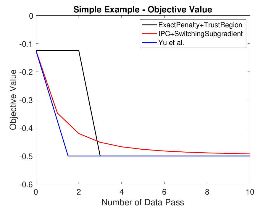
We leave additional details on the experiments’ setting in Section A.5 due to the limit of space. The numerical results are presented in Figure 1 where $x$-axis represents the number of data passes each algorithm performed and $y$-axis denotes the objective value $f({\mathbf{x}})$ in the first row and the constraint value $g({\mathbf{x}})$ in the second row. As Figure 1 shows, the IPC method is comparable with the exact penalty method. However, the IPC method can be potentially applied to non-smooth constraints while the exact penalty method cannot. Although the algorithm by [53] also works well in these instances, it doesn’t have any theoretical guarantee for nonconvex constrained optimization problems. We also plot the objective value and the constraint value against the CPU time. Due to the limit of space, we put these Figures in Section A.5 in the supplementary file.

Appendix A Appendix

In this section, we provide the proofs for the theoretical results in the paper.

A.1 Proof of Lemma 1

Proof.

Note that ${\mathbf{x}}_{0}$ is an $\epsilon^{2}$-feasible solution. Using the definitions of $\mathcal{A}({\mathbf{x}}_{t},\hat{\rho},\hat{\epsilon},\delta/T)$ and $\hat{\epsilon}$ and the union bound, we can show that the iterate ${\mathbf{x}}_{t}$ generated by Algorithm 1 is an $\epsilon^{2}$-feasible solution for any $t$ with a probability of at least $1-\delta$.

Let $\tilde{\mathbf{x}}_{t}\equiv\mathop{\mathrm{arg\,min}{}}\limits_{{\mathbf{x}}\in\mathcal{X}}\{g({\mathbf{x}})+\frac{\hat{\rho}}{2}\|{\mathbf{x}}-{\mathbf{x}}_{t}\|^{2}\}$. According to Assumption 1B, the fact that ${\mathbf{x}}_{t}$ is $\epsilon^{2}$-feasible, and the fact that $\hat{\rho}\leq\rho+\rho_{\epsilon}$, we have

$$-\sigma_{\epsilon}\geq\min\limits_{{\mathbf{x}}\in\mathcal{X}}g({\mathbf{x}})+\frac{\rho+\rho_{\epsilon}}{2}\|{\mathbf{x}}-{\mathbf{x}}_{t}\|^{2}\geq\min\limits_{{\mathbf{x}}\in\mathcal{X}}g({\mathbf{x}})+\frac{\hat{\rho}}{2}\|{\mathbf{x}}-{\mathbf{x}}_{t}\|^{2}=g(\tilde{\mathbf{x}}_{t})+\frac{\hat{\rho}}{2}\|\tilde{\mathbf{x}}_{t}-{\mathbf{x}}_{t}\|^{2}.$$ (11)

As a result, the Lagrangian multiplier $\lambda_{t}$ is well-defined and satisfies the optimality condition below together with $\widehat{\mathbf{x}}_{t}$:

$$\mathbf{0}\in\partial f(\widehat{\mathbf{x}}_{t})+\hat{\rho}(\widehat{\mathbf{x}}_{t}-{\mathbf{x}}_{t})+\lambda_{t}(\partial g(\widehat{\mathbf{x}}_{t})+\hat{\rho}(\widehat{\mathbf{x}}_{t}-{\mathbf{x}}_{t}))+\widehat{\bm{\zeta}}_{t},$$ (12)

for some $\widehat{\bm{\zeta}}_{t}\in\mathcal{N}_{\mathcal{X}}(\widehat{\mathbf{x}}_{t})$.

Since $g({\mathbf{x}})+\frac{\hat{\rho}}{2}\|{\mathbf{x}}-{\mathbf{x}}_{t}\|^{2}+\mathbf{1}_{\mathcal{X}}({\mathbf{x}})$ is $(\hat{\rho}-\rho)$-strongly convex in ${\mathbf{x}}$ and $\frac{\widehat{\bm{\zeta}}_{t}}{\lambda_{t}}\in\mathcal{N}_{\mathcal{X}}(\widehat{\mathbf{x}}_{t})=\partial\mathbf{1}_{\mathcal{X}}(\widehat{\mathbf{x}}_{t})$, we have

$$g(\tilde{\mathbf{x}}_{t})+\frac{\hat{\rho}}{2}\|\tilde{\mathbf{x}}_{t}-{\mathbf{x}}_{t}\|^{2} \geq g(\widehat{\mathbf{x}}_{t})+\frac{\hat{\rho}}{2}\|\widehat{\mathbf{x}}_{t}-{\mathbf{x}}_{t}\|^{2}+\langle\partial g(\widehat{\mathbf{x}}_{t})+\hat{\rho}(\widehat{\mathbf{x}}_{t}-{\mathbf{x}}_{t})+\frac{\widehat{\bm{\zeta}}_{t}}{\lambda_{t}},\tilde{\mathbf{x}}_{t}-\widehat{\mathbf{x}}_{t}\rangle+\frac{\hat{\rho}-\rho}{2}\|\tilde{\mathbf{x}}_{t}-\widehat{\mathbf{x}}_{t}\|^{2}$$

$$\geq\langle\partial g(\widehat{\mathbf{x}}_{t})+\hat{\rho}(\widehat{\mathbf{x}}_{t}-{\mathbf{x}}_{t})+\widehat{\bm{\zeta}}_{t}/\lambda_{t},\tilde{\mathbf{x}}_{t}-\widehat{\mathbf{x}}_{t}\rangle+\frac{\hat{\rho}-\rho}{2}\|\tilde{\mathbf{x}}_{t}-\widehat{\mathbf{x}}_{t}\|^{2}.$$

Applying (11) to the inequality above and arranging terms give

$$-\sigma_{\epsilon}-\frac{(\hat{\rho}-\rho)\|\tilde{\mathbf{x}}_{t}-\widehat{\mathbf{x}}_{t}\|^{2}}{2} \geq\langle\partial g(\widehat{\mathbf{x}}_{t})+\hat{\rho}(\widehat{\mathbf{x}}_{t}-{\mathbf{x}}_{t})+\widehat{\bm{\zeta}}_{t}/\lambda_{t},\tilde{\mathbf{x}}_{t}-\widehat{\mathbf{x}}_{t}\rangle$$

$$\geq-\frac{\|\partial g(\widehat{\mathbf{x}}_{t})+\hat{\rho}(\widehat{\mathbf{x}}_{t}-{\mathbf{x}}_{t})+\widehat{\bm{\zeta}}_{t}/\lambda_{t}\|^{2}}{2(\hat{\rho}-\rho)}-\frac{(\hat{\rho}-\rho)\|\tilde{\mathbf{x}}_{t}-\widehat{\mathbf{x}}_{t}\|^{2}}{2},$$

which implies $\|\partial g(\widehat{\mathbf{x}}_{t})+\hat{\rho}(\widehat{\mathbf{x}}_{t}-{\mathbf{x}}_{t})+\widehat{\bm{\zeta}}_{t}/\lambda_{t}\|^{2}\geq 2\sigma_{\epsilon}(\hat{\rho}-\rho)$.

Using this lower bound on $\|\partial g(\widehat{\mathbf{x}}_{t})+\hat{\rho}(\widehat{\mathbf{x}}_{t}-{\mathbf{x}}_{t})+\widehat{\bm{\zeta}}_{t}/\lambda_{t}\|^{2}$ and (12), we have that

$$\lambda_{t}=\frac{\|\partial f(\widehat{\mathbf{x}}_{t})+\hat{\rho}(\widehat{\mathbf{x}}_{t}-{\mathbf{x}}_{t})\|}{\|\partial g(\widehat{\mathbf{x}}_{t})+\hat{\rho}(\widehat{\mathbf{x}}_{t}-{\mathbf{x}}_{t})+\widehat{\bm{\zeta}}_{t}/\lambda_{t}\|}\leq\frac{M+\hat{\rho}D}{\sqrt{2\sigma_{\epsilon}(\hat{\rho}-\rho)}}$$

for all $t$ with a probability of at least $1-\delta$, where we have used Assumption 1C and Assumption 1F in the inequality. ∎

A.2 Proof of Theorem 1

Proof.

Since ${\mathbf{x}}_{t+1}=\mathcal{A}({\mathbf{x}}_{t},\hat{\rho},\hat{\epsilon},\delta/T)$, the definition of $\mathcal{A}$ and the union bound imply that the following inequalities hold for $t=0,\dots,T-1$ with a probability of at least $1-\delta$.

$$f({\mathbf{x}}_{t+1})+\frac{\hat{\rho}}{2}\|{\mathbf{x}}_{t+1}-{\mathbf{x}}_{t}\|^{2}-f(\widehat{\mathbf{x}}_{t})-\frac{\hat{\rho}}{2}\|\widehat{\mathbf{x}}_{t}-{\mathbf{x}}_{t}\|^{2}\leq\hat{\epsilon}^{2},\hskip 9.24994ptg({\mathbf{x}}_{t+1})+\frac{\hat{\rho}}{2}\|{\mathbf{x}}_{t+1}-{\mathbf{x}}_{t}\|^{2}\leq\hat{\epsilon}^{2}.$$ (13)

Let $\lambda_{t}$ be the optimal Lagrangian multiplier corresponding to $\widehat{\mathbf{x}}_{t}$. Then $\widehat{\mathbf{x}}_{t}$ is also the optimal solution of the Lagrangian function $\mathcal{L}({\mathbf{x}})\equiv f({\mathbf{x}})+\frac{\hat{\rho}}{2}\|{\mathbf{x}}-{\mathbf{x}}_{t}\|^{2}+\lambda_{t}(g({\mathbf{x}})+\frac{\hat{\rho}}{2}\|{\mathbf{x}}-{\mathbf{x}}_{t}\|^{2})$. Since $\mathcal{L}({\mathbf{x}})$ is $(1+\lambda_{t})(\hat{\rho}-\rho)$-strongly convex, we have

$$\frac{(1+\lambda_{t})(\hat{\rho}-\rho)}{2}\|{\mathbf{x}}_{t}-\widehat{\mathbf{x}}_{t}\|^{2} \leq f({\mathbf{x}}_{t})+\frac{\hat{\rho}}{2}\|{\mathbf{x}}_{t}-{\mathbf{x}}_{t}\|^{2}+\lambda_{t}(g({\mathbf{x}}_{t})+\frac{\hat{\rho}}{2}\|{\mathbf{x}}_{t}-{\mathbf{x}}_{t}\|^{2})$$ (14)

$$-\left[f(\widehat{\mathbf{x}}_{t})+\frac{\hat{\rho}}{2}\|\widehat{\mathbf{x}}_{t}-{\mathbf{x}}_{t}\|^{2}+\lambda_{t}(g(\widehat{\mathbf{x}}_{t})+\frac{\hat{\rho}}{2}\|\widehat{\mathbf{x}}_{t}-{\mathbf{x}}_{t}\|^{2})\right]$$

$$= f({\mathbf{x}}_{t})-f(\widehat{\mathbf{x}}_{t})+\lambda_{t}g({\mathbf{x}}_{t})-\frac{\hat{\rho}}{2}\|\widehat{\mathbf{x}}_{t}-{\mathbf{x}}_{t}\|^{2},$$

where we use the complementary slackness, i.e., $\lambda_{t}(g(\widehat{\mathbf{x}}_{t})+\frac{\hat{\rho}}{2}\|\widehat{\mathbf{x}}_{t}-{\mathbf{x}}_{t}\|^{2})=0$ in the equality above. Organizing the terms in the first inequality of (13), we get

$$f({\mathbf{x}}_{t+1}) \leq f(\widehat{\mathbf{x}}_{t})+\hat{\epsilon}^{2}+\frac{\hat{\rho}}{2}\|\widehat{\mathbf{x}}_{t}-{\mathbf{x}}_{t}\|^{2}-\frac{\hat{\rho}}{2}\|{\mathbf{x}}_{t+1}-{\mathbf{x}}_{t}\|^{2}$$

$$\leq f(\widehat{\mathbf{x}}_{t})+\hat{\epsilon}^{2}+f({\mathbf{x}}_{t})-f(\widehat{\mathbf{x}}_{t})+\lambda_{t}g({\mathbf{x}}_{t})-\frac{(1+\lambda_{t})(\hat{\rho}-\rho)}{2}\|{\mathbf{x}}_{t}-\widehat{\mathbf{x}}_{t}\|^{2}$$

$$=f({\mathbf{x}}_{t})+\lambda_{t}g({\mathbf{x}}_{t})-\frac{(1+\lambda_{t})(\hat{\rho}-\rho)}{2}\|{\mathbf{x}}_{t}-\widehat{\mathbf{x}}_{t}\|^{2}+\hat{\epsilon}^{2}$$

where second inequality is because of (14). The inequality above can be written as

$$\frac{(1+\lambda_{t})(\hat{\rho}-\rho)}{2}\|{\mathbf{x}}_{t}-\widehat{\mathbf{x}}_{t}\|^{2}\leq f({\mathbf{x}}_{t})-f({\mathbf{x}}_{t+1})+\lambda_{t}g({\mathbf{x}}_{t})+\hat{\epsilon}^{2}$$ (15)

Summing up inequality (15) from $t=0,1,\dots,T-1$, we have

$$\sum_{t=0}^{T-1}\frac{(1+\lambda_{t})(\hat{\rho}-\rho)}{2}\|{\mathbf{x}}_{t}-\widehat{\mathbf{x}}_{t}\|^{2}\leq f({\mathbf{x}}_{0})-f_{\text{lb}}+\sum_{t=0}^{T-1}\lambda_{t}g({\mathbf{x}}_{t})+T\hat{\epsilon}^{2},$$

where $f_{\text{lb}}$ is introduced in Assumption 1D. Note that $g({\mathbf{x}}_{t})\leq g({\mathbf{x}}_{t})+\frac{\hat{\rho}}{2}\|{\mathbf{x}}_{t}-{\mathbf{x}}_{t-1}\|^{2}\leq\hat{\epsilon}^{2}$ because of the property of $\mathcal{A}$. So we have

$$\sum_{t=0}^{T-1}\frac{(\hat{\rho}-\rho)}{2}\|{\mathbf{x}}_{t}-\widehat{\mathbf{x}}_{t}\|^{2}\leq\sum_{t=0}^{T-1}\frac{(1+\lambda_{t})(\hat{\rho}-\rho)}{2}\|{\mathbf{x}}_{t}-\widehat{\mathbf{x}}_{t}\|^{2}\leq f({\mathbf{x}}_{0})-f_{\text{lb}}+\sum_{t=0}^{T-1}\lambda_{t}\hat{\epsilon}^{2}+T\hat{\epsilon}^{2}.$$

Dividing both sides by $T(\hat{\rho}-\rho)/2$, we have

$$\mathbb{E}_{R}\|{\mathbf{x}}_{R}-\widehat{\mathbf{x}}_{R}\|^{2}=\frac{1}{T}\sum_{t=0}^{T-1}\|{\mathbf{x}}_{t}-\widehat{\mathbf{x}}_{t}\|^{2} \leq\frac{2(f({\mathbf{x}}_{0})-f_{\text{lb}})}{T(\hat{\rho}-\rho)}+\frac{2}{T(\hat{\rho}-\rho)}\sum_{t=0}^{T-1}(1+\lambda_{t})\hat{\epsilon}^{2}$$

$$\leq\frac{2(f({\mathbf{x}}_{0})-f_{\text{lb}})}{T(\hat{\rho}-\rho)}+\frac{2\hat{\epsilon}^{2}}{(\hat{\rho}-\rho)}\left(\frac{M+\hat{\rho}D}{\sqrt{2\sigma_{\epsilon}(\hat{\rho}-\rho)}}+1\right)$$

$$\leq\frac{\epsilon^{2}}{2}+\frac{\epsilon^{2}}{2}=\epsilon^{2}$$

with a probability of at least $1-\delta$, where the second inequality is by Lemma 1 and the last inequality follows the definitions of $T$ and $\hat{\epsilon}$. ∎

A.3 Proof of Theorem 2

Proof.

For simplicity of notation, we defined $\mu:=\hat{\rho}-\rho$. Let $J:=\{0,1,\dots,K-1\}\backslash I$ where $I$ is generated in Algorithm 2 when it terminates.

Suppose $k\in I$, namely, $G({\mathbf{z}}_{k})\leq\hat{\epsilon}^{2}$ is satisfied in iteration $k$. Algorithm 2 will update ${\mathbf{z}}_{k+1}$ using $F^{\prime}({\mathbf{z}}_{k})$. Following the standard analysis of subgradient decent method, we can get

$$F({\mathbf{z}}_{k})-F(\widehat{\mathbf{x}}_{t}) \leq\gamma_{k}(M^{2}+\hat{\rho}D^{2})+(\frac{1}{2\gamma_{k}}-\frac{\mu}{2})\|{\mathbf{z}}_{k}-\widehat{\mathbf{x}}_{t}\|^{2}-\frac{\|{\mathbf{z}}_{k+1}-\widehat{\mathbf{x}}_{t}\|^{2}}{2\gamma_{k}}$$

$$=\frac{2(M^{2}+\hat{\rho}D^{2})}{\mu(k+2)}+(\frac{\mu(k+2)}{4}-\frac{2\mu}{4})\|{\mathbf{z}}_{k}-\widehat{\mathbf{x}}_{t}\|^{2}-\frac{\mu(k+2)}{4}\|{\mathbf{z}}_{k+1}-\widehat{\mathbf{x}}_{t}\|^{2}$$

$$=\frac{2(M^{2}+\hat{\rho}D^{2})}{\mu(k+2)}+\frac{\mu k}{4}\|{\mathbf{z}}_{k}-\widehat{\mathbf{x}}_{t}\|^{2}-\frac{\mu(k+2)}{4}\|{\mathbf{z}}_{k+1}-\widehat{\mathbf{x}}_{t}\|^{2}$$ (16)

Multiplying $k+1$ to the both sides of 16, we can get

$$(k+1)(F({\mathbf{z}}_{k})-F(\widehat{\mathbf{x}}_{t})) \leq\frac{2(M^{2}+\hat{\rho}D^{2})(k+1)}{\mu(k+2)}+\frac{\mu k(k+1)}{4}\|{\mathbf{z}}_{k}-\widehat{\mathbf{x}}_{t}\|^{2}-\frac{\mu(k+1)(k+2)}{4}\|{\mathbf{z}}_{k+1}-\widehat{\mathbf{x}}_{t}\|^{2}$$

$$\leq\frac{2(M^{2}+\hat{\rho}D^{2})}{\mu}+\frac{\mu k(k+1)}{4}\|{\mathbf{z}}_{k}-\widehat{\mathbf{x}}_{t}\|^{2}-\frac{\mu(k+1)(k+2)}{4}\|{\mathbf{z}}_{k+1}-\widehat{\mathbf{x}}_{t}\|^{2}$$ (17)

Suppose $k\in J$, namely, $G({\mathbf{z}}_{k})\leq\hat{\epsilon}^{2}$ is not satisfied in iteration $k$. Algorithm 2 will update ${\mathbf{z}}_{k+1}$ using $G^{\prime}({\mathbf{z}}_{k})$. Similarly, we can get

$$(k+1)(G({\mathbf{z}}_{k})-G(\widehat{\mathbf{x}}_{t}))\leq\frac{2(M^{2}+\hat{\rho}D^{2})}{\mu}+\frac{\mu k(k+1)}{4}\|{\mathbf{z}}_{k}-\widehat{\mathbf{x}}_{t}\|^{2}-\frac{\mu(k+1)(k+2)}{4}\|{\mathbf{z}}_{k+1}-\widehat{\mathbf{x}}_{t}\|^{2}$$ (18)

Summing up inequalities (17) and (18) from $k=0,\dots,K-1$ and dropping the non-negative terms, we obtain

$$\sum\limits_{k\in I}(k+1)(F({\mathbf{z}}_{k})-F(\widehat{\mathbf{x}}_{t}))+\sum\limits_{k\in J}(k+1)(G({\mathbf{z}}_{k})-G(\widehat{\mathbf{x}}_{t})) \leq\frac{2K(M^{2}+\hat{\rho}D^{2})}{\mu}$$ (19)

Because $G({\mathbf{z}}_{k})>\hat{\epsilon}^{2}$ when $k\in J$ and $G(\widehat{\mathbf{x}}_{t})\leq 0$, the inequality above implies

$$\sum\limits_{k\in I}(k+1)(F({\mathbf{z}}_{k})-F(\widehat{\mathbf{x}}_{t}))+\sum\limits_{k\in J}(k+1)\hat{\epsilon}^{2} \leq\frac{2K(M^{2}+\hat{\rho}D^{2})}{\mu}$$ (20)

Rearranging terms gives

$$\sum_{k\in I}(k+1)(F({\mathbf{z}}_{k})-F(\widehat{\mathbf{x}}_{t})) \leq\sum_{k\in I}(k+1)\hat{\epsilon}^{2}-\sum_{k=0}^{K-1}(k+1)\hat{\epsilon}^{2}+\frac{2K(M^{2}+\hat{\rho}D^{2})}{\mu}$$

$$\leq\sum_{k\in I}(k+1)\hat{\epsilon}^{2}-\frac{K(K+1)}{2}\hat{\epsilon}^{2}+\frac{2K(M^{2}+\hat{\rho}D^{2})}{\mu}.$$

Given that $K\geq\frac{4(M^{2}+\hat{\rho}D^{2})}{\mu\hat{\epsilon}^{2}}$, the summation of the last two terms in the inequality above is non-positive. As a result, we have

$$\sum_{k\in I}(k+1)(F({\mathbf{z}}_{k})-F(\widehat{\mathbf{x}}_{t}))\leq\sum_{k\in I}(k+1)\hat{\epsilon}^{2}$$

Dividing both sides by $\sum_{k\in I}(k+1)$ and using the convexity of $F$, we obtain $F({\mathbf{x}}_{t+1})-F(\widehat{\mathbf{x}}_{t})\leq\hat{\epsilon}^{2}$. As the same time, the convexity of $G$ ensures $G({\mathbf{x}}_{t+1})\leq\frac{\sum_{k\in I}(k+1)G({\mathbf{z}}_{k})}{\sum_{k\in I}(k+1)}\leq\hat{\epsilon}^{2}$.

Hence, Algorithm 2 can be used as an oracle to solve (9) and the complexity of Algorithm 1 will be

$$TK=O\left(\frac{(f({\mathbf{x}}_{0})-f_{\text{lb}})(M^{2}+\hat{\rho}D^{2})}{\epsilon^{4}(\hat{\rho}-\rho)^{3}}\Big(\frac{M+\hat{\rho}D}{\sqrt{\sigma_{\epsilon}(\hat{\rho}-\rho)}}+1\Big)\right).$$

Note that, Algorithm 2 is deterministic so that the complexity above does not depend on $\delta$. ∎

A.4 Proof of Theorem 3

Proof.

According to Assumption 1B and the factor that ${\mathbf{x}}_{t}$ is $\epsilon^{2}$-feasible with a high probability, Assumption 2 (The Slater’s condition) in [53] holds for the subproblem (9) with a high probability. According to Theorem 4 in [53], Algorithm 3 guarantees

$$F({\mathbf{x}}_{t+1})-F(\widehat{\mathbf{x}}_{t})\leq\mathcal{B}_{1}(D,\tilde{M}_{0},\tilde{M}_{1},m,\sigma_{\epsilon},K,\delta)$$ (21)

with a probability of at least $1-\delta$, where

$$\mathcal{B}_{1}(D,\tilde{M}_{0},\tilde{M}_{1},m,\sigma_{\epsilon},K,\delta)$$ (22)

$$\equiv \frac{D^{2}+\tilde{M}_{1}^{2}/4+(\tilde{M}_{0}+\sqrt{m}\tilde{M}_{1}D)^{2}/2+\log^{0.5}\big(\frac{1}{\delta}\big)\tilde{M}_{0}\Lambda(D,\tilde{M}_{0},\tilde{M}_{1},m,\sigma_{\epsilon},K,\delta)}{\sqrt{K}},$$

$$\Lambda(D,\tilde{M}_{0},\tilde{M}_{1},m,\sigma_{\epsilon},K,\delta) \equiv \frac{\sigma_{\epsilon}}{2}+(\tilde{M}_{0}+\sqrt{m}\tilde{M}_{1}D)+\frac{2D^{2}}{\sigma_{\epsilon}}+\frac{2\tilde{M}_{1}D+(\tilde{M}_{0}+\sqrt{m}\tilde{M}_{1}D)^{2}}{\sigma_{\epsilon}}$$ (23)

$$+\tilde{\Lambda}(D,\tilde{M}_{0},\tilde{M}_{1},m,\sigma_{\epsilon},K,\delta)+\frac{8(\tilde{M}_{0}+\sqrt{m}\tilde{M}_{1}D)^{2}}{\sigma_{\epsilon}}\log\big(\frac{2K}{\delta}\big)=O(\log(K/\delta)),$$

and

$$\tilde{\Lambda}(D,\tilde{M}_{0},\tilde{M}_{1},m,\sigma_{\epsilon},K,\delta) \equiv \frac{8(\tilde{M}_{0}+\sqrt{m}\tilde{M}_{1}D)^{2}}{\sigma_{\epsilon}}\log\left[1+\frac{32(\tilde{M}_{0}+\sqrt{m}\tilde{M}_{1}D)^{2}}{\sigma_{\epsilon}^{2}}\exp\left(\frac{\sigma_{\epsilon}}{8(\tilde{M}_{0}+\sqrt{m}\tilde{M}_{1}D)}\right)\right].$$

According to equation (22) in [53], Algorithm 3 guarantees

$$F_{i}({\mathbf{x}}_{t+1}) \leq \frac{\|(Q_{K}^{1},Q_{K}^{2},\dots,Q_{K}^{m})\|}{K}+\frac{\tilde{M}_{1}^{2}}{\sqrt{K}}+\frac{\sqrt{m}\tilde{M}_{1}^{2}}{2K^{2}}\sum_{k=0}^{K-1}\|(Q_{k}^{1},Q_{k}^{2},\dots,Q_{k}^{m})\|$$ (24)

for $i=1,\dots,m$. It is also shown in Theorem 3 in [53] that

$$\|(Q_{k}^{1},Q_{k}^{2},\dots,Q_{k}^{m})\| \leq \sqrt{K}\Lambda(D,\tilde{M}_{0},\tilde{M}_{1},m,\sigma_{\epsilon},K,\delta)$$ (25)

for $k=0,1,\dots,K$ with a probability of at least $1-\delta$. Applying (25) to (24) and organizing terms, we obtain

$$F_{i}({\mathbf{x}}_{t+1}) \leq \mathcal{B}_{2}(D,\tilde{M}_{0},\tilde{M}_{1},m,\sigma_{\epsilon},K,\delta)$$ (26)

with a probability of at least $1-\delta$, where

$$\mathcal{B}_{2}(D,\tilde{M}_{0},\tilde{M}_{1},m,\sigma_{\epsilon},K,\delta)$$ (27)

$$\equiv \frac{\Lambda(D,\tilde{M}_{0},\tilde{M}_{1},m,\sigma_{\epsilon},K,\delta)+\tilde{M}_{1}^{2}+\Lambda(D,\tilde{M}_{0},\tilde{M}_{1},m,\sigma_{\epsilon},K,\delta)\sqrt{m}\tilde{M}_{1}^{2}/2}{\sqrt{K}}$$

To ensure Algorithm 3 is an oracle for (9), it suffices to choose the $K$ large enough so that the left hand sides of (21) and (26) are both no more than $\hat{\epsilon}^{2}$. Because $\Lambda(D,\tilde{M}_{0},\tilde{M}_{1},m,\sigma_{\epsilon},K,\delta)=O(\log(K/\delta))$. It suffices to choose $K=\tilde{O}(\frac{1}{\hat{\epsilon}^{4}}\log(\frac{1}{\delta}))$. Hence, Algorithm 3 can be used as an oracle to solve (9) and the complexity of Algorithm 1 will be

$$TK=\tilde{O}\left(\frac{1}{\epsilon^{6}}\right).$$

∎

A.5 Additional Numerical Results

Figure 2: Experiments Results for Problems with Fairness Constraint

We choose $\hat{\epsilon}=10^{-2}$ in the IPC method. For all instances except Simple Example, the three algorithms in comparison all start at a solution ${\mathbf{x}}_{0}$ constructed by projecting an all-one vector to $\mathcal{X}=\{{\mathbf{x}}\in\mathbb{R}^{d}|\|{\mathbf{x}}\|_{1}\leq 20\}$. We confirm that ${\mathbf{x}}_{0}$ is a feasible solution for these three real instances so that Assumption 1E is satisfied. For Simple Example, the initial solution is chosen to be $(0,0.5)^{T}$. The subproblem in the IPC method is solved by Algorithm 2 with the number of iterations $K=\frac{1}{\hat{\epsilon}^{2}}$. We assume $\hat{\rho}=2\rho$ in our algorithm for all experiments and, since $\rho$ is unknown, we select the best value for $\hat{\rho}$ from a discrete grid of candidates according to the performance of algorithm. Eventually, the value $\hat{\rho}=10^{-2.5}$ leads to a good performance on all three real datasets. Therefore, $\hat{\rho}=10^{-2.5}$ is used to create Figure 1 and Figure 2. To be fair, the control parameters in the exact penalty method [6] and the (deterministic) subgradient method [53] are also tuned instead of chosen as their theoretical values in their papers.

Additional numerical results are presented in Figure 2 where $x$-axis represents the CPU time and $y$-axis denotes the objective value in the first row and the constraint value in the second row. In terms of CPU time, the IPC method is also comparable with the exact penalty method.

References

- [1] Z. Allen-Zhu. Natasha: Faster non-convex stochastic optimization via strongly non-convex parameter. In Proceedings of the 34th International Conference on Machine Learning (ICML), pages 89–97, 2017.
- [2] Z. Allen-Zhu and E. Hazan. Variance reduction for faster non-convex optimization. In Proceedings of the 33nd International Conference on Machine Learning (ICML), pages 699–707, 2016.
- [3] A. Bayandina, P. Dvurechensky, A. Gasnikov, F. Stonyakin, and A. Titov. Mirror descent and convex optimization problems with non-smooth inequality constraints. In Large-Scale and Distributed Optimization, pages 181–213. Springer, 2018.
- [4] D. P. Bertsekas. Nonlinear programming. Athena scientific Belmont, 1999.
- [5] D. P. Bertsekas. Constrained optimization and Lagrange multiplier methods. Academic press, 2014.
- [6] C. Cartis, N. I. Gould, and P. L. Toint. On the evaluation complexity of composite function minimization with applications to nonconvex nonlinear programming. SIAM Journal on Optimization, 21(4):1721–1739, 2011.
- [7] C. Cartis, N. I. Gould, and P. L. Toint. On the complexity of finding first-order critical points in constrained nonlinear optimization. Mathematical Programming, 144(1-2):93–106, 2014.
- [8] J. Chen, T. Yang, Q. Lin, L. Zhang, and Y. Chang. Optimal stochastic strongly convex optimization with a logarithmic number of projections. In Proceedings of the Thirty-Second Conference on Uncertainty in Artificial Intelligence, pages 122–131. AUAI Press, 2016.
- [9] Z. Chen, T. Yang, J. Yi, B. Zhou, and E. Chen. Universal stagewise learning for non-convex problems with convergence on averaged solutions. CoRR, /abs/1808.06296, 2018.
- [10] A. Cotter, H. Jiang, and K. Sridharan. Two-player games for efficient non-convex constrained optimization. arXiv preprint arXiv:1804.06500, 2018.
- [11] K. Crammer and Y. Singer. On the learnability and design of output codes for multiclass problems. Machine learning, 47(2-3):201–233, 2002.
- [12] D. Davis and D. Drusvyatskiy. Complexity of finding near-stationary points of convex functions stochastically. arXiv preprint arXiv:1802.08556, 2018.
- [13] D. Davis and D. Drusvyatskiy. Stochastic model-based minimization of weakly convex functions. arXiv preprint arXiv:1803.06523, 2018.
- [14] D. Davis and D. Drusvyatskiy. Stochastic subgradient method converges at the rate on weakly convex functions. arXiv preprint arXiv:1802.02988, 2018.
- [15] D. Davis and B. Grimmer. Proximally guided stochastic subgradient method for nonsmooth, nonconvex problems. arXiv preprint arXiv:1707.03505, 2017.
- [16] D. Drusvyatskiy. The proximal point method revisited. arXiv preprint arXiv:1712.06038, 2017.
- [17] D. Drusvyatskiy and C. Paquette. Efficiency of minimizing compositions of convex functions and smooth maps. Mathematical Programming, Jul 2018.
- [18] O. Fercoq, A. Alacaoglu, I. Necoara, and V. Cevher. Almost surely constrained convex optimization. arXiv preprint arXiv:1902.00126, 2019.
- [19] S. Ghadimi and G. Lan. Stochastic first- and zeroth-order methods for nonconvex stochastic programming. SIAM Journal on Optimization, 23(4):2341–2368, 2013.
- [20] S. Ghadimi and G. Lan. Accelerated gradient methods for nonconvex nonlinear and stochastic programming. Math. Program., 156(1-2):59–99, 2016.
- [21] G. Goh, A. Cotter, M. Gupta, and M. P. Friedlander. Satisfying real-world goals with dataset constraints. In Advances in Neural Information Processing Systems, pages 2415–2423, 2016.
- [22] S. Lacoste-Julien. Convergence rate of frank-wolfe for non-convex objectives. arXiv preprint arXiv:1607.00345, 2016.
- [23] S. Lacoste-Julien, M. Schmidt, and F. Bach. A simpler approach to obtaining an o (1/t) convergence rate for the projected stochastic subgradient method. arXiv preprint arXiv:1212.2002, 2012.
- [24] G. Lan and Y. Yang. Accelerated stochastic algorithms for nonconvex finite-sum and multi-block optimization. CoRR, abs/1805.05411, 2018.
- [25] G. Lan and Z. Zhou. Algorithms for stochastic optimization with expectation constraints. arXiv preprint arXiv:1604.03887, 2016.
- [26] Q. Lin, M. Liu, H. Rafique, and T. Yang. Solving weakly-convex-weakly-concave saddle-point problems as weakly-monotone variational inequality. arXiv preprint arXiv:1810.10207, 2018.
- [27] Q. Lin, R. Ma, and T. Yang. Level-set methods for finite-sum constrained convex optimization. In International Conference on Machine Learning, pages 3118–3127, 2018.
- [28] Q. Lin, S. Nadarajah, and N. Soheili. A level-set method for convex optimization with a feasible solution path. SIAM Journal on Optimization, 28(4):3290–3311, 2018.
- [29] P.-L. Loh et al. Statistical consistency and asymptotic normality for high-dimensional robust -estimators. The Annals of Statistics, 45(2):866–896, 2017.
- [30] M. Mahdavi, T. Yang, R. Jin, and S. Zhu. Stochastic gradient descent with only one projection. In Advances in Neural Information Processing Systems (NIPS), pages 503–511, 2012.
- [31] Y. Nesterov. Introductory lectures on convex optimization: A basic course, volume 87. Springer Science & Business Media, 2013.
- [32] J. Nocedal and S. Wright. Numerical optimization. Springer Science & Business Media, 2006.
- [33] C. Paquette, H. Lin, D. Drusvyatskiy, J. Mairal, and Z. Harchaoui. Catalyst for gradient-based nonconvex optimization. pages 1–10, 2018.
- [34] B. Polyak. A general method of solving extremum problems. Soviet Mathematics Doklady, 8(3):593–597, 1967.
- [35] H. Rafique, M. Liu, Q. Lin, and T. Yang. Non-convex min-max optimization: Provable algorithms and applications in machine learning. arXiv preprint arXiv:1810.02060, 2018.
- [36] S. J. Reddi, A. Hefny, S. Sra, B. Póczós, and A. Smola. Stochastic variance reduction for nonconvex optimization. In Proceedings of the 33rd International Conference on International Conference on Machine Learning (ICML), pages 314–323. JMLR.org, 2016.
- [37] S. J. Reddi, S. Sra, B. Póczos, and A. J. Smola. Fast incremental method for smooth nonconvex optimization. In 55th IEEE Conference on Decision and Control (CDC), pages 1971–1977, 2016.
- [38] P. Rigollet and X. Tong. Neyman-pearson classification, convexity and stochastic constraints. Journal of Machine Learning Research, 12(Oct):2831–2855, 2011.
- [39] R. Rockafellar. Convex Analysis. Princeton mathematical series. Princeton University Press, 1970.
- [40] R. T. Rockafellar. Monotone operators and the proximal point algorithm. SIAM J. on Control and Optimization, 14(5), 1976.
- [41] A. P. Ruszczyński. Nonlinear optimization, volume 13. Princeton university press, 2006.
- [42] S. Sahni. Computationally related problems. SIAM Journal on Computing, 3(4):262–279, 1974.
- [43] X. Wang, S. Ma, and Y.-x. Yuan. Penalty methods with stochastic approximation for stochastic nonlinear programming. Mathematics of Computation, 86(306):1793–1820, 2017.
- [44] X. Wei and M. J. Neely. Primal-dual frank-wolfe for constrained stochastic programs with convex and non-convex objectives. arXiv preprint arXiv:1806.00709, 2018.
- [45] X. Wei, H. Yu, Q. Ling, and M. Neely. Solving non-smooth constrained programs with lower complexity than : A primal-dual homotopy smoothing approach. In Advances in Neural Information Processing Systems, pages 3995–4005, 2018.
- [46] J. Weston and C. Watkins. Multi-class support vector machines. Technical report, Citeseer, 1998.
- [47] Y. Xu. First-order methods for constrained convex programming based on linearized augmented lagrangian function. arXiv preprint arXiv:1711.08020, 2017.
- [48] Y. Xu. Global convergence rates of augmented lagrangian methods for constrained convex programming. arXiv preprint arXiv:1711.05812, 2017.
- [49] Y. Xu. Primal-dual stochastic gradient method for convex programs with many functional constraints. arXiv preprint arXiv:1802.02724, 2018.
- [50] Y. Xu, S. Zhu, S. Yang, C. Zhang, R. Jin, and T. Yang. Learning with non-convex truncated losses by sgd. arXiv preprint arXiv:1805.07880, 2018.
- [51] T. Yang, Q. Lin, and Z. Li. Unified convergence analysis of stochastic momentum methods for convex and non-convex optimization. volume abs/1604.03257, 2016.
- [52] T. Yang, Q. Lin, and L. Zhang. A richer theory of convex constrained optimization with reduced projections and improved rates. In Proceedings of the 34th International Conference on Machine Learning-Volume 70, pages 3901–3910. JMLR. org, 2017.
- [53] H. Yu, M. Neely, and X. Wei. Online convex optimization with stochastic constraints. In Advances in Neural Information Processing Systems, pages 1428–1438, 2017.
- [54] H. Yu and M. J. Neely. A simple parallel algorithm with an o(1/t) convergence rate for general convex programs. SIAM Journal on Optimization, 27(2):759–783, 2017.
- [55] M. B. Zafar, I. Valera, M. Rodriguez, K. Gummadi, and A. Weller. From parity to preference-based notions of fairness in classification. In Advances in Neural Information Processing Systems, pages 229–239, 2017.
- [56] M. B. Zafar, I. Valera, M. G. Rodriguez, and K. P. Gummadi. Fairness constraints: Mechanisms for fair classification. arXiv preprint arXiv:1507.05259, 2015.
- [57] L. Zhang, T. Yang, R. Jin, and X. He. O (logt) projections for stochastic optimization of smooth and strongly convex functions. arXiv preprint arXiv:1304.0740, 2013.
- [58] S. Zhang and N. He. On the convergence rate of stochastic mirror descent for nonsmooth nonconvex optimization. arXiv preprint arXiv:1806.04781, 2018.