arXiv is now an independent nonprofit! Learn more
License: arXiv.org perpetual non-exclusive license
arXiv:1908.01241v3 [cs.LG] 10 Sep 2021

Robust Max Entrywise Error Bounds for Sparse Tensor Estimation via Similarity Based Collaborative Filtering

Devavrat Shah    Christina Lee Yu Note: Massachusetts Institute of Technology, Cambridge, MA; devavrat@mit.edu Note: Cornell University, Ithaca NY; cleeyu@cornell.edu
Abstract

Consider the task of estimating a 3-order n×n×nn\times n\times n tensor from noisy observations of randomly chosen entries in the sparse regime. We introduce a similarity based collaborative filtering algorithm for sparse tensor estimation and argue that it achieves sample complexity that nearly matches the conjectured computationally efficient lower bound on the sample complexity for the setting of low-rank tensors. Our algorithm uses the matrix obtained from the flattened tensor to compute similarity, and estimates the tensor entries using a nearest neighbor estimator. We prove that the algorithm recovers a low rank tensor with maximum entry-wise error (MEE) and mean-squared-error (MSE) decaying to 00 as long as each entry is observed independently with probability p=Ω(n3/2+κ)p=\Omega(n^{-3/2+\kappa}) for any arbitrarily small κ>0\kappa>0. More generally, we establish robustness of the estimator, showin that when arbitrary noise bounded by 𝜺0\boldsymbol{\varepsilon}\geq 0 is added to each observation, the estimation error with respect to MEE and MSE degrades by 𝗉𝗈𝗅𝗒(𝜺){\sf poly}(\boldsymbol{\varepsilon}). Consequently, even if the tensor may not have finite rank but can be approximated within 𝜺0\boldsymbol{\varepsilon}\geq 0 by a finite rank tensor, then the estimation error converges to 𝗉𝗈𝗅𝗒(𝜺){\sf poly}(\boldsymbol{\varepsilon}). Our analysis sheds insight into the conjectured sample complexity lower bound, showing that it matches the connectivity threshold of the graph used by our algorithm for estimating similarity between coordinates.

1 Introduction

Tensor estimation involves the task of predicting underlying structure in a high-dimensional tensor structured dataset given only a sparse subset of observations. We call this “tensor estimation” rather than the conventional “tensor completion” as the goal is not only to fill missing entries but also to estimate entries whose noisy observations are available. Whereas matrices represent data associated to two modes, rows and columns, tensors represent data associated to general dd modes. For example, a datapoint collected from a user-product interaction an e-commerce platform may be associated to a user, product, and date/time, which could be represented in a 3-order tensor where the three modes would correspond to users, products, and date/time. Image data is also naturally represented in a 3-order tensor format, with two modes representing the location of the pixel, and the third mode representing the RGB color components. Video data furthermore introduces a fourth mode indexing the time. Dynamic network data can also be represented in a tensor with one mode indexing the time and the other two modes indexing the nodes in the network.

There are many applications in which the dataset inherently has a lot of noise or is very sparsely observed. For example, e-commerce data is typically very sparse as the typical number of products a user interacts with is very small relative to the entire product catalog; furthermore the timepoints at which the user interacts with the platform may be sparse. When the dataset can be represented as a matrix, equivalent to a 2-order tensor, there has been a significant amount of research in designing practical algorithms and studying statistical limits for matrix estimation, a critical step in data pre-processing. Under conditions on uniform sampling and incoherence, the minimum sample complexity for estimation has been tightly characterized and achieved by simple algorithms. It is a natural and relevant question then to consider whether the techniques developed can extend to higher order tensors as well.

The previous literature has primarily focused on attaining consistency with respect to the mean squared error (MSE). Unfortunately as this is aggregated over the error in the full tensor, it does not translate to consistent bounds on entrywise error, as the error on a single entry could be very large despite the MSE being small due to averaging over many entries. However, entrywise bounds are important in practice as the results of tensor estimation are often used subsequently for decisions that involve comparisons between the estimates of individual entries.

In this work we focus on attaining consistent max entrywise error bounds by extending similarity based collaborative filtering algorithms to tensor estimation. Similarity based collaborative filtering is widely used in industry due to its simplicity, interpretability, and amenability to distributed and parallelized implementations. In the analysis of our proposed algorithm we show that it achieves a sample complexity that nearly matches a conjectured lower bound for computationally efficient algorithms. Perhaps most notably, our theoretical guarantees provide high probability bounds on the maximum entrywise error of the estimate, which is significantly stronger than the typical mean squared error style bounds found in the literature for other algorithms. We also provide error bounds under arbitrary bounded noise, which has implications towards approximately low rank settings.

1.1 Related Literature

Algorithms for analyzing sparse low rank matrices (equivalent to 2-order tensors) where the observations are sampled uniformly randomly have been well-studied. The algorithms consist of spectral decomposition or matrix factorization [19, 20, 8], nuclear norm minimization [5, 6, 7, 27, 25, 23], gradient descent [19, 20, 9, 29, 13], alternating minimization [17, 15], and nearest neighbor style collaborative filtering [14, 28, 21, 3, 4]. These algorithms have been shown to be provably consistent as long as the number of observations is Ω(rn𝗉𝗈𝗅𝗒(logn))\Omega(rn\,{\sf poly}(\log n)) for the noiseless setting where rr is the rank and nn is the number of rows and columns [19, 5]; similar results have been attained under additive Gaussian noise [20, 6] and generic bounded noise [8, 3]. Lower bounds show that Ω(rn)\Omega(rn) samples are necessary for consistent estimation, and Ω(rnlog(n))\Omega(rn\log(n)) samples are necessary for exact recovery [6, 7], implying that the proposed algorithms are nearly sample efficient order-wise up to the information theoretic lower bounds.

There are results extending matrix estimation algorithms to higher order tensor estimation, assuming the tensor is low rank and that observations are sampled uniformly at random. The earliest approaches simply flatten or unfold the tensor to a matrix and subsequently apply matrix estimation algorithms [22, 12, 30, 31]. A dd-order tensor where each dimension is length nn would be unfolded to a nd/2×nd/2n^{\lfloor d/2\rfloor}\times n^{\lceil d/2\rceil} matrix, resulting in a sample complexity of O(nd/2𝗉𝗈𝗅𝗒(logn))O(n^{\lceil d/2\rceil}\,{\sf poly}(\log n)), significantly larger than the natural statistical lower bound that is linear with nn due to the model being parameterized by linear in nn latent variables. When dd is odd, for example d=3d=3 the sample complexity for this naive approach scales as O(n2𝗉𝗈𝗅𝗒(logn))O(n^{2}\,{\sf poly}(\log n)).

Subsequent progress has shown that it is feasible to improve upon naive sample complexity bound obtained by unfolding the tensor to a matrix when dd is odd [18, 2, 33, 1, 26, 24]. For a 3-order tensor, they provide consistent estimators requiring only a sample complexity of Ω(n3/2𝗉𝗈𝗅𝗒(logn))\Omega(n^{3/2}\,{\sf poly}(\log n)). [18, 2] analyzes the alternating minimization algorithm for exact recovery of the tensor given noiseless observations and finite rank r=Θ(1)r=\Theta(1). [1, 26] use the sum of squares (SOS) method, and [24] introduces a spectral method. Both of these latter algorithms can handle noisy observations and overcomplete tensors where the rank is larger than the dimension. For a general dd-order tensor these results translate into a sample complexity scaling as O(nd/2)O(n^{d/2}), improving upon O(nd/2CLOSEO(n^{\lceil d/2\rceil}. [34] prove that tensor nuclear norm minimization can recover the underlying low-rank dd-order tensor with O(n3/2𝗉𝗈𝗅𝗒(logn))O(n^{3/2}\,{\sf poly}(\log n)) samples in the noiseless setting; however, the algorithm is not efficiently computable as computing tensor nuclear norm is NP-hard [11].

[1] conjecture that any polynomial time estimator for a 3-order tensor must require Ω(n3/2)\Omega(n^{3/2}) samples, based on a reduction between tensor estimation for a rank-1 tensor to the random 3-XOR distinguishability problem. They argue that if using the sum of squares hierarchy to construct relaxations for tensor rank, any result that achieves a consistent estimator with fewer than n3/2n^{3/2} samples will violate a conjectured hardness of random 3-XOR distinguishability. Information theoretic bounds imply that one needs at least Ω(drn)\Omega(drn) observations to recover a dd-order rank rr tensor, consistent with the degrees of freedom or number of parameters in the model. Interestingly, this implies a conjectured gap between the computational and statistically achievable sample complexities, highlighting how tensor estimation is disctinctly more difficult than matrix estimation.

1.2 Contribution

Our results answer the following unresolved questions in the literature.

  • 1.

    Is there a computationally efficient estimator that can provide a consistent estimation of low-rank tensor with respect to maximum entry-wise error (MEE) with minimal sample complexity of Ω(n32)\Omega(n^{\frac{3}{2}}) in the presence of noise?

  • 2.

    Is there an extension of matrix estimation collaborative filtering algorithm for the setting of tensor estimation that can provide consistent estimation with such minimal sample complexity?

  • 3.

    Can the estimator be robust to adversarial bounded noise in the observations?

To begin with, we propose an algorithm for a symmetric 33-order tensor estimation which generalizes an iterative nearest neighbor collaborative filtering algorithm for sparse matrix estimation introduced in [3]. As discussed, the iterative collaborative filtering for matrix estimation of [3] applied to the n×n2n\times n^{2} matrix obtained by unfolding the 33-order tensor does not work as it requires Ω(n2)\Omega(n^{2}) samples, far more than Ω(n32)\Omega(n^{\frac{3}{2}}) required per best known computationally efficient estimator, for consistent estimation. However, we argue that such a matrix obtained from the unfolded tensor can be used, after non-trivial modification, to compute the similarities between rows accurately using Ω(n32+κ)\Omega(n^{\frac{3}{2}+\kappa}) samples for any positive κ>0\kappa>0. And after computing these similarities, by using tensor structure through nearest neighbor, we can obtain consistent estimation.

Specifically, we establish that the mean squared error (MSE) in the estimation converges to 00 as long as Ω(n3/2+κ)\Omega(n^{3/2+\kappa}) random samples are observed for any κ>0\kappa>0 for tensor with rank r=Θ(1)r=\Theta(1). We further establish a stronger guarantee that the maximum entry-wise error (MEE) converge to 00 with high probability with similar sample complexity of Ω(n3/2+κ)\Omega(n^{3/2+\kappa}). Thus, this simple iterative collaborative filtering algorithm nearly achieves the conjectured computational sample complexity lower bound of Ω(n3/2)\Omega(n^{3/2}) for tensor estimation. While we present the results for symmetric tensors, our method and analysis can extend to asymmetric tensors, which we discuss in Section 5.4.

Beyond low-rank tensors, our results hold for tensors with potentially countably infinite rank as long as they can be well approximated by a low-rank tensor. Specifically, if the tensor can be approximated with 𝜺0\boldsymbol{\varepsilon}\geq 0 with respect to max-norm by a rank r=Θ(1)r=\Theta(1) tensor, then the MSE converges to 𝗉𝗈𝗅𝗒(𝜺){\sf poly}(\boldsymbol{\varepsilon}) and MEE converges to 𝗉𝗈𝗅𝗒(𝜺){\sf poly}(\boldsymbol{\varepsilon}) with high probability as long as Ω(n3/2+κ)\Omega(n^{3/2+\kappa}) random samples are observed for any κ>0\kappa>0. This follows as a consequence of the robustness property of the algorithm that we establish: if arbitrary noise bounded by 𝜺0\boldsymbol{\varepsilon}\geq 0 is added to each observation, then the estimation error with respect to MEE and MSE degrades by 𝗉𝗈𝗅𝗒(𝜺){\sf poly}(\boldsymbol{\varepsilon}).

To establish our results, the key analytic tool is utilizing certain concentration properties of a bilinear form arising from the local neighborhood expansion of any given coordinate for an asymmetric matrix with dimensions n×n2n\times n^{2}. This generalizes the analysis of a similar property for symmetric matrices in the prior work of [3]. Specifically, establishing the desired concentration requires handling dependencies arising in the local neighborhood expansion of the 33-order tensor that was absent in the matrix setting considered in [3]. Subsequently, we require a novel analytic method compared to the prior work. In particular we believe that the proof techniques in Lemma 7.7 may be useful to other settings in which one may desire a tighter concentration on sums of sparse random variables. As a consequence, we also establish performance guarantees for matrix estimation for asymmetric matrices having dimensions of different order, generalizing beyond of [3].

The algorithm and analysis also sheds insight on the conjectured lower bound for 33-order tensor. In particular, the threshold of n3/2n^{3/2} is precisely the density of observations needed for the connectivity in the associated graph that is utilized to calculate similarities. If the graph is disconnected, the similarities can not be computed, while if the graph is connected, we are able to show that similarity calculations yield an excellent estimator. Understanding this relationship further remains an interesting open research direction.

A benefit of our algorithm is that it can be implemented in a parallelized manner where the similarities between pair of indices are computed in parallel. This lends itself to a distributed, scalable implementation. A naive bound on sample complexity of our algorithm for 3-order tensor is at most pn6pn^{6}. As discussed in Section 5.4, with use of approximate nearest neighbors, these can be further improved and made truly implementable.

2 Preliminaries

Sparse tensor estimation hinges on an assumption that the true model exhibits low dimensional structure despite the high dimensional representation. However, there is not a unique definition of rank in the tensor setting, as natural generalizations of matrix rank lead to different quantities when extended to higher order tensors. We will focus on two commonly used definitions of tensor rank, the CP rank and the Tucker or multilinear rank.

For a dd-order tensor FndF\in\mathbb{R}^{n^{d}}, we can decompose FF into a sum of rank-1 tensors. For example if d=3d=3, then

F=k=1rukvkwk,F=\sum_{k=1}^{r}u_{k}\otimes v_{k}\otimes w_{k},

where {uk,vk,wk}k[r]\{u_{k},v_{k},w_{k}\}_{k\in[r]} is a collection of length nn vectors. The CP-rank is the minimum number rr such that FF can be written as a sum of rr rank-1 tensors, which we refer to as a CP-decomposition. The CP-rank may in fact be larger than the dimension nn, and furthermore the latent vectors need not be orthogonal as is the case in the matrix setting.

An alternate notion of tensor rank is defined according to the dimension of subspaces corresponding to each mode. Let F(y)F_{(y)} denote the unfolded tensor along the yy-th mode, which is a matrix of dimension n×nd1n\times n^{d-1}. Let columns of F(y)F_{(y)} be referred to as mode yy fibers of tensor FF as depicted in Figure 1.

Figure 1: Depicting an unfolding of a 3rd order tensor along mode 1. The columns of the resulting matrix are referred to as the mode-1 fibers of the tensor.

The Tucker rank, or multilinear rank, is a vector (r1,r2,rd)(r_{1},r_{2},\dots r_{d}) such that for each mode [d]\ell\in[d], rr_{\ell} is the dimension of the column space of F(y)F_{(y)}. The Tucker rank is also the minimal values of (r1,r2,rd)(r_{1},r_{2},\dots r_{d}) such that the tensor FF can be decomposed according to a multilinear multiplication of a core tensor Λr1×r2×rd\Lambda\in\mathbb{R}^{r_{1}\times r_{2}\times\dots r_{d}} with latent factor matrices Q1QdQ_{1}\dots Q_{d} for Qn×rQ_{\ell}\in\mathbb{R}^{n_{\ell}\times r_{\ell}}, denoted as

F=(Q1Qd)(Λ):=𝐤[r1]×[r2]××[rd]Λ(𝐤)Q1(,k1)Q2(,k2)Qd(,kd),\displaystyle F=(Q_{1}\otimes\cdots Q_{d})\cdot(\Lambda):=\sum_{{\bf k}\in[r_{1}]\times[r_{2}]\cdots\times[r_{d}]}\Lambda({\bf k})Q_{1}(\cdot,k_{1})\otimes Q_{2}(\cdot,k_{2})\cdots\otimes Q_{d}(\cdot,k_{d}), (2.1)

and depicted in Figure 2. The higher order SVD (HOSVD) specifies a unique Tucker decomposition in which the factor matrices Q1QdQ_{1}\dots Q_{d} are orthonormal and correspond to the left singular vectors of the unfolded tensor along each mode [10].

Figure 2: (Left) The tensor CP-rank admits a decomposition corresponding to the sum of rr rank-1 tensors.
(Right) The Tucker rank or multilinear rank (r1,r2,rt)(r_{1},r_{2},\dots r_{t}) admits a decomposition corresponding to a multilinear multiplication of a core tensor of dimensions (r1,r2,rd)(r_{1},r_{2},\dots r_{d}) with latent factor matrices associated to each mode.

If the CP-rank is rr, the Tucker-rank is bounded above by (r,r,r)(r,r,\dots r) by constructing a superdiagonal core tensor. If the Tucker rank is (r1,r2,rt)(r_{1},r_{2},\dots r_{t}), the CP-rank is bounded by the number of nonzero entries in the core tensor, which is at most r1r2rt/(maxr)r_{1}r_{2}\cdots r_{t}/(\max_{\ell}r_{\ell}) [10]. While the latent factors of the HOSVD are orthogonal, the latent factors corresponding to the minimal CP-decomposition may not be orthogonal. For simplicity of presentation, we will consider a limited setting where there exists a decomposition of the tensor into the sum of orthogonal rank-1 tensors. This is equivalent to enforcing that the core tensor Λ\Lambda associated to the Tucker decomposition is superdiagonal, or equivalently enforcing that the latent factors in the minimal CP-decomposition are orthogonal. There does not always exist such an orthogonal CP-decomposition, however this class still includes all rank 1 tensors which encompasses the class of instances used to construct the hardness conjecture in [1]. Our results also extend beyond to general tensors as well, though the presentation is simpler in the orthogonal setting.

3 Problem Statement and Model

Consider an n×n×nn\times n\times n symmetric tensor FF generated as follows: For each u[n]u\in[n], sample θuU[0,1]\theta_{u}\sim U[0,1] independently. Let the true underlying tensor FF be described by a Lipschitz function ff evaluated over the latent variables, F(u,v,w)=f(θu,θv,θw)F(u,v,w)=f(\theta_{u},\theta_{v},\theta_{w}) for u,v,w[n]u,v,w\in[n]. Without loss of generality, we shall assume that supu,v,w[0,1]|f(θu,θv,θw)|1\sup_{u,v,w\in[0,1]}|f(\theta_{u},\theta_{v},\theta_{w})|\leq 1.

Let MM denote the observed symmetric data tensor, and let Ω[n]3\Omega\subseteq[n]^{3} denote the set of observed indices. Due to the symmetry, it is sufficient to restrict the index set to triplets (u,v,w)(u,v,w) such that uvwu\leq v\leq w, as the datapoint is identical for all other permutations of the same triplet. The datapoint at each of these distinct triplets {(u,v,w):uvw}\{(u,v,w):u\leq v\leq w\} is observed independently with probability p(0,1]p\in(0,1], where we assume the observation is corrupted by mean zero independent additive noise terms. For (u,v,w)Ω(u,v,w)\in\Omega,

M(u,v,w)\displaystyle M(u,v,w) =F(u,v,w)+ϵuvw,\displaystyle=F(u,v,w)+\epsilon_{uvw}, (3.1)

and for (u,v,w)Ω(u,v,w)\notin\Omega, M(u,v,w)=M(u,v,w)=\star11 1 The notation of \star is used to denote the missing observation. When convenient, we shall replace \star by 00 for the purpose of computation. . We allow ϵuvw\epsilon_{uvw} to have different distributions for different distinct triplets (u,v,w)(u,v,w) as long as the variance is uniformly bounded by σ2\sigma^{2}. We shall assume that |M(u,v,w)|1|M(u,v,w)|\leq 1 with probability 11. The techniques and the results presented here can likely be extended for setting where ϵuvw\epsilon_{uvw} is sub Gaussian rather than uniformly bounded. The goal is to recover the underlying tensor FF from the incomplete noisy observation MM so that the mean squared error (MSE) is small, where MSE for an estimate F^\hat{F} is defined as

MSE(F^):=𝔼[1n3(u,v,w)[n]3(F^(u,v,w)F(u,v,w))2].\displaystyle\text{MSE}(\hat{F}):=\mathbb{E}\left[\tfrac{1}{n^{3}}\textstyle\sum_{(u,v,w)\in[n]^{3}}(\hat{F}(u,v,w)-F(u,v,w))^{2}\right]. (3.2)

We will also interested in the maximum entry-wise error (MEE) defined as

FF^max:=max(u,v,w)[n]3|F^(u,v,w)F(u,v,w)|.\displaystyle\|F-\hat{F}\|_{\max}:=\max_{(u,v,w)\in[n]^{3}}|\hat{F}(u,v,w)-F(u,v,w)|. (3.3)

3.1 Finite spectrum

Consider the setting where the function ff has finite spectrum. That is,

f(u,v,w)=k=1rλkqk(θu)qk(θv)qk(θw),f(u,v,w)=\textstyle\sum_{k=1}^{r}\lambda_{k}q_{k}(\theta_{u})q_{k}(\theta_{v})q_{k}(\theta_{w}),

where r=Θ(1)r=\Theta(1) and qk(.)q_{k}(.) denotes the orthonormal 2\ell_{2} eigenfunctions, satisfying 01qk(θ)2𝑑θ=1\int_{0}^{1}q_{k}(\theta)^{2}d\theta=1 and 01qk(θ)qh(θ)𝑑θ=0 for kh\int_{0}^{1}q_{k}(\theta)q_{h}(\theta)d\theta=0\text{ for }k\neq h. Assume that the eigenfunctions are bounded, i.e. |qk(θ)|B|q_{k}(\theta)|\leq B for all k[r]k\in[r].

Let Λ\Lambda denote the diagonal r×rr\times r matrix where Λkk=λk\Lambda_{kk}=\lambda_{k}. Let QQ denote the r×nr\times n matrix where Qka=qk(θa)Q_{ka}=q_{k}(\theta_{a}). Let 𝒬\mathcal{Q} denote the r×(n2)r\times\binom{n}{2} matrix where 𝒬kb=qk(θb1)qk(θb2)\mathcal{Q}_{kb}=q_{k}(\theta_{b_{1}})q_{k}(\theta_{b_{2}}) for some b(n2)b\in\binom{n}{2} that represents the pair of vertices (b1,b2)(b_{1},b_{2}) for b1<b2b_{1}<b_{2}. The finite spectrum assumption for ff implies that the sampled tensor FF is such that,

F=k=1rλk(QTek)(QTek)(QTek).F=\textstyle\sum_{k=1}^{r}\lambda_{k}(Q^{T}e_{k})\otimes(Q^{T}e_{k})\otimes(Q^{T}e_{k}).

That is, FF has CP-rank at most rr. In above and in the remainder of the paper, eke_{k} denotes a vector with all 00s but kkth entry being 11 of appropriate dimension (here it is rr).

3.2 Approximately finite spectrum

In general, ff may not have finite spectrum, e.g. a generic analytic function ff. For such a setting, we shall consider ff with approximately finite spectrum. Specifically, a function f:[0,1]3f:[0,1]^{3}\to\mathbb{R}, it is said to have 𝜺\boldsymbol{\varepsilon}-approximate finite spectrum with rank rr for 𝜺0\boldsymbol{\varepsilon}\geq 0 if there exists a symmetric function fr:[0,1]3f_{r}:[0,1]^{3}\to\mathbb{R} such that

supθu,θv,θw[0,1]|f(θu,θv,θw)fr(θu,θv,θw)|𝜺\displaystyle\sup_{\theta_{u},\theta_{v},\theta_{w}\in[0,1]}|f(\theta_{u},\theta_{v},\theta_{w})-f_{r}(\theta_{u},\theta_{v},\theta_{w})|\leq\boldsymbol{\varepsilon}
Fr(u,v,w)=fr(θu,θv,θw)=k=1rλkqk(θu)qk(θv)qk(θw),\displaystyle F_{r}(u,v,w)=f_{r}(\theta_{u},\theta_{v},\theta_{w})=\textstyle\sum_{k=1}^{r}\lambda_{k}q_{k}(\theta_{u})q_{k}(\theta_{v})q_{k}(\theta_{w}), (3.4)

where r=Θ(1)r=\Theta(1) and qk(.)q_{k}(.) denotes the orthonormal 2\ell_{2} eigenfunctions as before. That is, they satisfy 01qk(θ)2𝑑θ=1\int_{0}^{1}q_{k}(\theta)^{2}d\theta=1, 01qk(θ)qh(θ)𝑑θ=0 for kh\int_{0}^{1}q_{k}(\theta)q_{h}(\theta)d\theta=0\text{ for }k\neq h and |qk(θ)|B|q_{k}(\theta)|\leq B for all k[r]k\in[r].

The above describe property of ff implies that the sampled tensor FF is has 𝜺\boldsymbol{\varepsilon}-approximate rank rr such that Fr=k=1rλk(QTek)(QTek)(QTek)F_{r}=\textstyle\sum_{k=1}^{r}\lambda_{k}(Q^{T}e_{k})\otimes(Q^{T}e_{k})\otimes(Q^{T}e_{k}) and

FFrmax\displaystyle\|F-F_{r}\|_{\max} 𝜺.\displaystyle\leq\boldsymbol{\varepsilon}.

3.3 Extensions Beyond Orthogonal CP-rank

The orthogonality conditions on our latent variable decomposition imply that the tensor FF can be written as a sum of rr rank-1 tensors, where the latent factors are approximately orthogonal. Alternately, this would suggest a Tucker decomposition of the tensor where the core tensor is superdiagonal. This assumption can be relaxed as the main property that our algorithm and analysis use is the orthogonal decomposition of the unfolded tensors along each mode. In the general setting, we would instead carry out the analysis with respect to the latent orthogonal factors corresponding to the SVD of the unfolded tensor into a matrix.

3.4 Comparision of Assumptions with Literature

In the decomposition of the model ff when it has finite spectrum, we assume that the functions qkq_{k} are orthonormal. This induces a decomposition of tensor FF in terms of Qr×nQ\in\mathbb{R}^{r\times n} with respect to the sampled latent features θU[0,1]\theta\sim U[0,1]. The rank rr of the underlying decomposition is assumed to be Θ(1)\Theta(1). We compare and contrast these with those assumed in the tensor estimation literature.

Most literature on tensor estimation do not impose a distribution on the underlying latent variables, but instead assume deterministic ‘incoherence’ style conditions on the latent singular vectors associated to the underlying tensor decomposition. This plays a similar role to our combined assumption of qkq_{k} being orthonormal and the latent variables sampled from a uniform distribution so that the mass in the singular vector matrix is roughly uniformly spread.

Some of the literature on tensor estimation allows for overcomplete tensors, i.e. r>nr>n. While our finite spectrum setup requires r=Θ(1)r=\Theta(1), the approximately finite spectrum can allow for potentially countably infinite spectrum but with sharply decaying spectrum so that it has 𝜺\boldsymbol{\varepsilon}-approximate rank being r=Θ(1)r=\Theta(1).

It is worth taking a note of the fact that to establish our result for the approximately finite spectrum setting, we perform a perturbation analysis wherein each observed entry is perturbed arbitrarily bounded by 𝜺\boldsymbol{\varepsilon} in magnitude: we shall establish that the resulting estimation error is changed by 𝗉𝗈𝗅𝗒(𝜺){\sf poly}(\boldsymbol{\varepsilon}), both with respect to the MSE and max-norm. That is, with respect to arbitrary bounded noise in the observations, we are able to characterize the error induced by our method, which is of interest in its own right.

We remark on the Lipschitz property of ff: the Lipschitz assumption implies that the tensor is “smooth”, and thus there are sets of rows and columns that are similar to one another. As our algorithm is based on a nearest neighbor style approach we need that for any coordinate uu, there is a significant mass of other coordinates aa that are similar to uu with respect to the function behavior. Other regularity conditions beyond Lipschitz that would also guarantee sufficiently many “nearest neighbors” would lead to similar results for our algorithm.

4 Algorithm

The algorithm is a nearest neighbor style in which the first phase is to estimate a distance function between coordinates, denoted dist(u,a)\text{{\sf dist}}(u,a) for all (u,a)[n]2(u,a)\in[n]^{2}. Given the similarities, for some threshold η\eta, the algorithm estimates by averaging datapoints from coordinates (a,b,c)(a,b,c) for which dist(u,a)η\text{{\sf dist}}(u,a)\leq\eta, dist(v,b)η\text{{\sf dist}}(v,b)\leq\eta, and dist(w,c)η\text{{\sf dist}}(w,c)\leq\eta.

The entry F(a,b,c)F(a,b,c) depends on a coordinate aa through its representation in the eigenspace, given by QeaQe_{a}. Therefore f(a,b,c)f(u,v,w)f(a,b,c)\approx f(u,v,w) as long as QeuQeaQe_{u}\approx Qe_{a}, QevQebQe_{v}\approx Qe_{b}, and QewQecQe_{w}\approx Qe_{c}. Ideally we would like our distance function dist(u,a)\text{{\sf dist}}(u,a) to approximate QeuQea2\|Qe_{u}-Qe_{a}\|_{2}, but these are hidden latent features that we do not have direct access to.

Let’s start with a thought experiment supposing that the density of observations were p=ω(n1)p=\omega(n^{-1}) and the noise variance is σ2\sigma^{2} for all entries. For a pair of coordinates uu and aa, the expected number of pairs (b,c)(b,c) such that both (u,b,c)(u,b,c) and (a,b,c)(a,b,c) are observed is on the order of p2n2=ω(1)p^{2}n^{2}=\omega(1). For fixed θa,θu\theta_{a},\theta_{u}, and for randomly sampled θb,θc\theta_{b},\theta_{c}, the expected squared difference between the two corresponding datapoints reflects the distance between QeaQe_{a} and QeuQe_{u} along with the overall level of noise,

𝔼[(M(a,b,c)M(u,b,c))2|θa,θu]\displaystyle\mathbb{E}[(M(a,b,c)-M(u,b,c))^{2}~|~\theta_{a},\theta_{u}]
=𝔼[(F(a,b,c)F(u,b,c))2|θa,θu]+𝔼[ϵabc2+ϵubc2]\displaystyle=\mathbb{E}[(F(a,b,c)-F(u,b,c))^{2}~|~\theta_{a},\theta_{u}]+\mathbb{E}[\epsilon_{abc}^{2}+\epsilon_{ubc}^{2}]
=𝔼[(kλk(qk(θa)qk(θu))qk(θb)qk(θc))2|θa,θu]+2σ2\displaystyle=\mathbb{E}[(\textstyle\sum_{k}\lambda_{k}(q_{k}(\theta_{a})-q_{k}(\theta_{u}))q_{k}(\theta_{b})q_{k}(\theta_{c}))^{2}~|~\theta_{a},\theta_{u}]+2\sigma^{2}
=𝔼[kλk2(qk(θa)qk(θu))2qk(θb)2qk(θc)2|θa,θu]+2σ2\displaystyle=\mathbb{E}[\textstyle\sum_{k}\lambda_{k}^{2}(q_{k}(\theta_{a})-q_{k}(\theta_{u}))^{2}q_{k}(\theta_{b})^{2}q_{k}(\theta_{c})^{2}~|~\theta_{a},\theta_{u}]+2\sigma^{2}
=kλk2(qk(θa)qk(θu))2+σ2\displaystyle=\textstyle\sum_{k}\lambda_{k}^{2}(q_{k}(\theta_{a})-q_{k}(\theta_{u}))^{2}+\sigma^{2}
=ΛQ(eaeu)22+2σ2,\displaystyle=\|\Lambda Q(e_{a}-e_{u})\|_{2}^{2}+2\sigma^{2},

where we use the fact that qk()q_{k}(\cdot) are orthonormal. This suggests that approximating dist(u,a)\text{{\sf dist}}(u,a) with the average squared difference between datapoints corresponding to pairs (b,c)(b,c) for which both (u,b,c)(u,b,c) and (a,b,c)(a,b,c) are observed.

This method does not attain the p=n3/2p=n^{-3/2} sample complexity, as the expected number of pairs (b,c)(b,c) for which (a,b,c)(a,b,c) and (u,b,c)(u,b,c) are both observed will go to zero for p=o(n1)p=o(n^{-1}). This limitation arises due to the fact that when p=o(n1)p=o(n^{-1}), the observations are extremely sparse. Consider the n×(n2)n\times\binom{n}{2} “flattened” matrix of the tensor where row uu correspond to coordinates u[n]u\in[n], and columns correspond to pairs of indices, e.g. (b,c)[n]×[n](b,c)\in[n]\times[n] with bcb\leq c. For any given row uu, there are very few other rows that share observations along any column with the given row uu, i.e. the number of ‘neighbors’ of any row index is few. If we wanted to exploit the intuition of the above simple calculations, we have to somehow enrich the neighborhood; and allow for noise terms in each entry to have different distributions and variance. We do so by constructing a graph using the non-zero pattern of the matrix as an adjacency matrix. This mirrors the idea from [3] for matrix estimation, which approximates distances by comparing expanded local neighborhoods in the graph representing the sparsity pattern of the unfolded or flattened tensor. A key distinction is that the tensor setting requires an important modification of how one constructs the local breadth-first-search (BFS) trees, described in step 3 below.

4.1 Formal Description

We provide a formal description of the algorithm below. The crux of the algorithm is to compute similarity between any pair of indices using the matrix obtained by flattening the tensor, and then using a nearest neighbor estimator using these similarities between indices over the tensor structure. Details are as follows.

Step 1: Sample Splitting. Let us assume for simplicity of the analysis that we obtain 22 independent fresh observation sets of the data, Ω1{\Omega_{1}} and Ω2{\Omega_{2}}. Tensors M1M_{1} and M2{M_{2}} contain information from the subset of the data in MM associated to Ω1{\Omega_{1}} and Ω2{\Omega_{2}} respectively. M1M_{1} is used to compute pairwise similarities between coordinates, and M2{M_{2}} is used to average over datapoints for the final estimate. Furthermore, we take the coordinates [n][n] and split it into two sets, [n]={1,2,,n/2}{n/2+1,n/2+2,n}[n]=\{1,2,\dots,n/2\}\cup\{n/2+1,n/2+2,\dots n\}. Without loss of generality, let’s assume that nn is even. Let 𝒱A\mathcal{V}_{A} denote the set of coordinate pairs within set 1 consisting of distinct coordinates, i.e. 𝒱A={(b,c)[n/2]2s.t.b<c}\mathcal{V}_{A}=\{(b,c)\in[n/2]^{2}~s.t.~b<c\}. Let 𝒱B\mathcal{V}_{B} denote the set of coordinate pairs within set 2 consisting of distinct coordinates, i.e. 𝒱B={(b,c)([n][n/2])2s.t.b<c}\mathcal{V}_{B}=\{(b,c)\in([n]\setminus[n/2])^{2}~s.t.~b<c\}. The sizes of |𝒱A||\mathcal{V}_{A}| and |𝒱B||\mathcal{V}_{B}| are both equal to (n/22)\binom{n/2}{2}. We define MA{M_{A}} to be the nn-by-(n/22)\binom{n/2}{2} matrix taking values MA(a,(b,c))=M1(a,b,c){M_{A}}(a,(b,c))=M_{1}(a,b,c), where each row corresponds to an original coordinate of the tensor, and each column corresponds to a pair of coordinates (b,c)𝒱A(b,c)\in\mathcal{V}_{A} from the original tensor. We define MB{M_{B}} to be the nn-by-(n/22)\binom{n/2}{2} matrix taking values MB(a,(b,c))=M1(a,b,c){M_{B}}(a,(b,c))=M_{1}(a,b,c), where each row corresponds to an original coordinate of the tensor, and each column corresponds to a pair of coordinates (b,c)𝒱B(b,c)\in\mathcal{V}_{B} from the original tensor. A row-column pair in the matrix corresponds to a triplet of coordinates in the original tensor. We will use matrices MA{M_{A}} and MB{M_{B}} to compute similarities or distances between coordinates, and we use tensor M2{M_{2}} to compute the final estimates via nearest neighbor averaging.

Step 2: Construct Bipartite Graph from Ω1,MA{\Omega_{1}},{M_{A}}. We define a bipartite graph corresponding to the flattened matrix MA{M_{A}}. Construct a graph with vertex set [n]𝒱A[n]\cup\mathcal{V}_{A}. There is an edge between vertex a[n]a\in[n] and vertex (b,c)𝒱A(b,c)\in\mathcal{V}_{A} if (a,b,c)Ω1(a,b,c)\in{\Omega_{1}}, and the corresponding weight of the edge is M1(a,b,c)M_{1}(a,b,c). Recall that we assumed a symmetric model such that triplets that are permutations of one another will have the same data entry and thus the same edge weight in the associated graph. Figure 3(a) provides a concrete example of a bipartite graph constructed from tensor observations.

Step 3: Expanding the Neighborhood. Consider the graph constructed from Ω1,MA{\Omega_{1}},{M_{A}}. For each vertex u[n]u\in[n], we construct a breadth first search (BFS) tree rooted at vertex uu such that the vertices for each depth of the BFS tree consists only of new and previously unvisited coordinates, i.e. if vertex a[n]a\in[n] is first visited at depth 4 of the BFS tree, then no vertex corresponding to (a,b)(a,b) for any b[n]b\in[n] can be visited in any subsequent depths greater than 4. Similarly, if (a,b)(a^{\prime},b^{\prime}) is visited in the BFS tree at depth 3, then vertices that include either of these coordinates, i.e. aa^{\prime}, bb^{\prime}, (a,c)(a^{\prime},c), or (b,c)(b^{\prime},c) for any c[n]c\in[n], can not be visited in subsequent depths greater than 3. This restriction is only across different depths; we allow (a,b)(a,b) and (a,c)(a,c) to be visited at the same depth of the BFS tree.

There may be multiple valid BFS trees due to different ordering of visiting edges at the same depth. For example, if a vertex at depth ss has edges to two different vertices at depth s1s-1 (i.e. two potential parents), only one of the edges can be chosen to maintain the tree property, but either choice is equally valid. Let us assume that when there is more than one option, one of the valid edges are chosen uniformly at random. Figure 3(c) shows valid BFS trees for a bipartite graph constructed from an example tensor.

The graph is bipartite so that each subsequent layer of the BFS tree alternates between the vertex sets [n][n] and 𝒱A\mathcal{V}_{A}. Consider a valid BFS tree rooted at vertex u[n]u\in[n] which respects the constraint that no coordinate is visited more than once. We will use 𝒰u,s𝒱A\mathcal{U}_{u,s}\subseteq\mathcal{V}_{A} to denote the set of vertices at depth (2s1)(2s-1) of the BFS tree, and we use 𝒮u,s[n]\mathcal{S}_{u,s}\subseteq[n] to denote the set of vertices at depth 2s2s of the BFS tree. Let u,s[n]𝒱A\mathcal{B}_{u,s}\subset[n]\cup\mathcal{V}_{A} denote the set of vertices which are visited in the first ss layers of the BFS tree,

u,s=hs/2𝒮u,hls/2𝒰u,l.\mathcal{B}_{u,s}=\cup_{h\in\lfloor s/2\rfloor}\mathcal{S}_{u,h}\cup_{l\in\lceil s/2\rceil}\mathcal{U}_{u,l}.

We will overload notation and sometimes use u,s\mathcal{B}_{u,s} to denote the subset of coordinates in [n][n] visited in the first ss layers of the BFS tree, including both visited single coordinate vertices or coordinates in vertices 𝒱A\mathcal{V}_{A}, i.e.

u,s=hs/2𝒮u,h{x[n]s.t.(y,z)ls/2𝒰u,l satisfying x{y,z}}.\mathcal{B}_{u,s}=\cup_{h\in\lfloor s/2\rfloor}\mathcal{S}_{u,h}~\cup~\left\{x\in[n]~\text{s.t.}~\exists(y,z)\in\cup_{l\in\lceil s/2\rceil}\mathcal{U}_{u,l}\text{ satisfying }x\in\{y,z\}\right\}.

Let 𝒢(u,s)\mathcal{G}(\mathcal{B}_{u,s}) denote all the information corresponding to the subgraph restricted to the first ss layers of the BFS tree rooted at uu. This includes the vertex set u,s\mathcal{B}_{u,s}, the latent variables {θa}au,s\{\theta_{a}\}_{a\in\mathcal{B}_{u,s}} and the edge weights {M1(a,b,c)}a,(b,c)u,s\{M_{1}(a,b,c)\}_{a,(b,c)\in\mathcal{B}_{u,s}}.

We define neighborhood vectors which represent the different layers of the BFS tree. Let Nu,s[0,1]nN_{u,s}\in[0,1]^{n} be associated to set 𝒮u,s\mathcal{S}_{u,s}, where the aa-th coordinate is equal to the product of weights along the path from uu to aa in the BFS tree for a𝒮u,sa\in\mathcal{S}_{u,s}. Similarly, let Wu,s[0,1]𝒱AW_{u,s}\in[0,1]^{\mathcal{V}_{A}} be associated to set 𝒰u,s\mathcal{U}_{u,s}, where the (b,c)(b,c)-th coordinate is equal to the product of weights along the path from uu to (b,c)(b,c) in the BFS tree for (b,c)𝒰u,s(b,c)\in\mathcal{U}_{u,s}. For a[n]a\in[n], let πu(a)\pi_{u}(a) denote the parent of aa in the valid BFS tree rooted at vertex uu. For (b,c)𝒱A(b,c)\in\mathcal{V}_{A}, let πu(b,c)\pi_{u}(b,c) denote the parent of (b,c)(b,c) in the BFS tree rooted at vertex uu. We can define the neighborhood vectors recursively,

Nu,s(a)\displaystyle N_{u,s}(a) =MA(a,πu(a))Wu,s(πu(a))𝕀(a𝒮u,s)\displaystyle={M_{A}}(a,\pi_{u}(a))W_{u,s}(\pi_{u}(a))\mathbb{I}_{(a\in\mathcal{S}_{u,s})}
Wu,s(b,c)\displaystyle W_{u,s}(b,c) =MA(πu(b,c),(b,c))Nu,s1(πu(b,c))𝕀((b,c)𝒰u,s)\displaystyle={M_{A}}(\pi_{u}(b,c),(b,c))N_{u,s-1}(\pi_{u}(b,c))\mathbb{I}_{((b,c)\in\mathcal{U}_{u,s})}

and Nu,0=euN_{u,0}=e_{u}. Let N~u,s\tilde{N}_{u,s} denote the normalized vector N~u,s=Nu,s/|𝒮u,s|\tilde{N}_{u,s}=N_{u,s}/|\mathcal{S}_{u,s}| and let W~u,s\tilde{W}_{u,s} denote the normalized vector W~u,s=Wu,s/|𝒰u,s|\tilde{W}_{u,s}=W_{u,s}/|\mathcal{U}_{u,s}|. Figure 3(d) illustrates the neighborhood sets and vectors for a valid BFS tree.
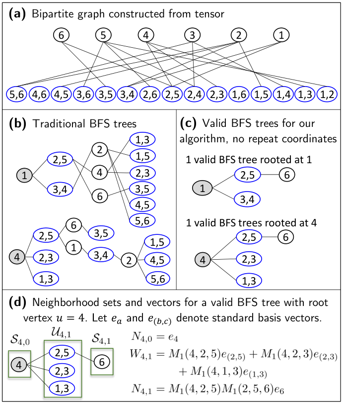
Refer to caption
Figure 3: Consider a symmetric 3-order tensor with n=6n=6, and the observation set Ω1={(1,3,4),(1,2,5),(2,3,4),(2,4,5),(2,5,6),(3,5,6)}\Omega_{1}=\{(1,3,4),(1,2,5),(2,3,4),(2,4,5),(2,5,6),(3,5,6)\}. Figure (a) depicts the bipartite graph constructed from this set of observations. Weights would be assigned to edges based on the value of the observed entry in the tensor M1M_{1}. Figure (b) depicts the traditional notion of the BFS tree rooted at vertices 1 and 4. Vertices at layer/depth ss correspond to vertices with shortest path distance of ss to the root vertex. Figure (c) depicts valid BFS trees for our algorithm, which imposes an additional constraint that coordinates cannot be repeated across depths. For the BFS tree rooted at vertex 1, edges ((2,5),4)((2,5),4) and ((3,4),2)((3,4),2) are not valid, as coordinates 2 and 4 have both been visited in layer 2 by the vertices (2,5)(2,5) and (3,4)(3,4). For the BFS tree rooted at vertex 4, edge ((2,5),1)((2,5),1) is not valid as coordinate 1 has been visited in layer 2 by the vertex (1,3)(1,3) and edge (6,(3,5))(6,(3,5)) is not valid as coordinates 4 and 5 have both been visited in layer 2. Figure (d) depicts the sets 𝒮u,s\mathcal{S}_{u,s} and 𝒰u,s\mathcal{U}_{u,s} along with the neighborhood vectors Nu,sN_{u,s} and Wu,sW_{u,s} for a specific valid BFS tree rooted at vertex u=4u=4.

Step 4: Computing the distances using MB{M_{B}}. Let

t\displaystyle t =ln(n)2ln(p2n3).\displaystyle=\Big\lceil\frac{\ln(n)}{2\ln(p^{2}n^{3})}\Big\rceil. (4.1)

A heuristic for the distance would be

dist(u,v)1|𝒱B|p2(N~u,tN~v,t)MBMBT(N~u,tN~v,t)\displaystyle\text{{\sf dist}}(u,v)~\approx\frac{1}{|\mathcal{V}_{B}|p^{2}}(\tilde{N}_{u,t}-\tilde{N}_{v,t}){M_{B}}{M_{B}}^{T}(\tilde{N}_{u,t}-\tilde{N}_{v,t}) (4.2)
=1|𝒱B|p2(α,β)𝒱Ba,b[n]2(N~u,t(a)N~v,t(a))MB(a,α,β)MB(b,α,β)(N~u,t(b)N~v,t(b))\displaystyle=\frac{1}{|\mathcal{V}_{B}|p^{2}}\sum_{(\alpha,\beta)\in\mathcal{V}_{B}}\sum_{a,b\in[n]^{2}}(\tilde{N}_{u,t}(a)-\tilde{N}_{v,t}(a)){M_{B}}(a,\alpha,\beta){M_{B}}(b,\alpha,\beta)(\tilde{N}_{u,t}(b)-\tilde{N}_{v,t}(b))

For technical reasons that facilitate cleaner analysis, we use the following distance calculations. There are two deviations from the equation in (4.2). First we exclude a=ba=b from the summation. Second we exclude coordinates for α\alpha or β\beta that have been visited previously in u,2t\mathcal{B}_{u,2t} or v,2t\mathcal{B}_{v,2t}.Define distance as

dist(u,v)\displaystyle\text{{\sf dist}}(u,v) =(Zuu+ZvvZuvZvu),\displaystyle=(Z_{uu}+Z_{vv}-Z_{uv}-Z_{vu}), (4.3)
Zuv\displaystyle Z_{uv} =1|𝒱B(u,v,t)|p2|𝒮u,t||𝒮v,t|(α,β)𝒱B(u,v,t)T~uv(α,β),\displaystyle=\frac{1}{|\mathcal{V}_{B}(u,v,t)|p^{2}|\mathcal{S}_{u,t}||\mathcal{S}_{v,t}|}\sum_{(\alpha,\beta)\in\mathcal{V}_{B}(u,v,t)}\tilde{T}_{uv}(\alpha,\beta),
𝒱B(u,v,t)\displaystyle\mathcal{V}_{B}(u,v,t) ={(α,β)𝒱Bs.t.αu,2tv,2t and βu,2tv,2t},\displaystyle=\{(\alpha,\beta)\in\mathcal{V}_{B}~s.t.~\alpha\notin\mathcal{B}_{u,2t}\cup\mathcal{B}_{v,2t}\text{ and }\beta\notin\mathcal{B}_{u,2t}\cup\mathcal{B}_{v,2t}\},
Tuv(α,β)\displaystyle T_{uv}(\alpha,\beta) =ab[n]Nu,t(a)Nv,t(b)MB(a,(α,β))MB(b,(α,β)).\displaystyle=\sum_{a\neq b\in[n]}N_{u,t}(a)N_{v,t}(b){M_{B}}(a,(\alpha,\beta)){M_{B}}(b,(\alpha,\beta)).

Step 5: Averaging datapoints to produce final estimate. Let Ω2uvw{\Omega_{2}}_{uvw} denote the set of indices (a,b,c)(a,b,c) such that abca\leq b\leq c, (a,b,c)Ω2(a,b,c)\in{\Omega_{2}}, and the estimated distances dist(u,a)\text{{\sf dist}}(u,a), dist(v,b)\text{{\sf dist}}(v,b), dist(w,c)\text{{\sf dist}}(w,c) are all less than some chosen threshold parameter η\eta. The final estimate averages the datapoints corresponding to indices in Ω2uvw{\Omega_{2}}_{uvw},

F^(u,v,w)\displaystyle\hat{F}(u,v,w) =1|Ω2uvw|(a,b,c)Ω2uvwM2(a,b,c).\displaystyle=\tfrac{1}{|{\Omega_{2}}_{uvw}|}\textstyle\sum_{(a,b,c)\in{\Omega_{2}}_{uvw}}{M_{2}}(a,b,c). (4.5)

4.2 Difference between tensor and matrix setting

The modifications in the construction of the breadth-first-search (BFS) tree for the tensor setting relative to the matrix setting are critical to the analysis. If we simply considered the classical construction of a BFS tree in the associated bipartite graph (as the matrix setting uses), this would lead to higher variance and bias due to the correlations of vertices sharing common latent variables associated to the same underlying coordinates of the tensor. Alternatively, if one constructed a BFS tree by not allowing any coordinate of the tensor to be visited more than once, this would also lead to suboptimal results as it would throw away too many entries, limiting the computed statistic to only order nn data points. As a result our final algorithm, which allows for vertices with shared coordinates in the same depth of the BFS but not across different depths, is carefully chosen in order to break dependencies across different depths of the BFS tree, while still allowing for sufficient expansion in each depth.

5 Main Result

We provide an upper bound on the mean squared error (MSE) as well as the max entry-wise error (MEE) for the algorithm, showing that both the MSE and the MEE converge to zero as long as p=n3/2+κp=n^{-3/2+\kappa} for some κ>0\kappa>0. Our result implies that the simple variant of collaborative filtering algorithm based on estimating similarities produces a consistent estimator when the tensor latent function has finite spectrum or low rank. Further we show that it is robust to arbitrary, additive perturbation in that the estimation error increases by gracefully in the amount of perturbation. To the best of our knowledge, such robustness to arbitrary bounded additive noise with respect to max-norm estimation is first of its kind in the literature on tensor estimation.

5.1 Finite spectrum

We establish consistency of our estimator with respect to MSE and max-norm error of the algorithm when the underlying ff has finite spectrum, i.e. rank rr model with r=Θ(1)r=\Theta(1).

Theorem 5.1.

We assume that the function ff is rank rr, LL-Lipschitz and that θU[0,1]\theta\sim U[0,1]. Assume that p=n3/2+κp=n^{-3/2+\kappa} for some κ(0,12)\kappa\in(0,\frac{1}{2}). Let tt be defined according to (4.1). For any arbitrarily small ψ(0,min(κ,38))\psi\in(0,\min(\kappa,\frac{3}{8})), choose the threshold

η\displaystyle\eta =Θ(n(κψ)).\displaystyle=\Theta\left(n^{-(\kappa-\psi)}\right).

The algorithm produces estimates so that,

MSE =O(n(κψ))=O(nψ(p2n3)1/2),\displaystyle=O(n^{-(\kappa-\psi)})=O\left(\frac{n^{\psi}}{(p^{2}n^{3})^{1/2}}\right),

and

FF^max\displaystyle\|F-\hat{F}\|_{\max} =O(n(κψ)/2),\displaystyle=O(n^{-(\kappa-\psi)/2}),

with probability 1O(n4exp(Θ(n2ψ)))1-O\left(n^{4}\exp(-\Theta(n^{2\psi}))\right).

5.2 Approximately finite spectrum

For approximate rank rr model, we establish a natural perturbation result for the algorithm. Specifically, if the underlying model has 𝜺\boldsymbol{\varepsilon}-approximate rank rr, then we argue that the result of Theorem 5.1 remain true, both with respect to MSE and max-norm error, with perturbation amount of 𝗉𝗈𝗅𝗒(𝜺){\sf poly}(\boldsymbol{\varepsilon}).

Theorem 5.2.

We assume that the function ff has 𝛆\boldsymbol{\varepsilon}-approximate rank rr, LL-Lipschitz and that θU[0,1]\theta\sim U[0,1]. Assume that p=n3/2+κp=n^{-3/2+\kappa} for some κ(0,12)\kappa\in(0,\frac{1}{2}). Choosing tt according to (4.1), it follows that t=14κt=\lceil\frac{1}{4\kappa}\rceil. For any arbitrarily small ψ(0,min(κ,38))\psi\in(0,\min(\kappa,\frac{3}{8})), choose the threshold

η\displaystyle\eta =Θ(n(κψ)+t𝜺(1+𝜺)2t1+t2𝜺2(1+𝜺)4t2).\displaystyle=\Theta\left(n^{-(\kappa-\psi)}+t\boldsymbol{\varepsilon}(1+\boldsymbol{\varepsilon})^{2t-1}+t^{2}\boldsymbol{\varepsilon}^{2}(1+\boldsymbol{\varepsilon})^{4t-2}\right).

The algorithm produces estimates so that,

MSE =O(n(κψ)+t𝜺(1+𝜺)2t1+t2𝜺2(1+𝜺)4t2)\displaystyle=O(n^{-(\kappa-\psi)}+t\boldsymbol{\varepsilon}(1+\boldsymbol{\varepsilon})^{2t-1}+t^{2}\boldsymbol{\varepsilon}^{2}(1+\boldsymbol{\varepsilon})^{4t-2})
=O(nψ(p2n3)1/2+t𝜺(1+𝜺)2t1+t2𝜺2(1+𝜺)4t2),\displaystyle=O\left(\frac{n^{\psi}}{(p^{2}n^{3})^{1/2}}+t\boldsymbol{\varepsilon}(1+\boldsymbol{\varepsilon})^{2t-1}+t^{2}\boldsymbol{\varepsilon}^{2}(1+\boldsymbol{\varepsilon})^{4t-2}\right),

and

FF^max\displaystyle\|F-\hat{F}\|_{\max} =O(n(κψ)/2+t𝜺(1+𝜺)2t1+t𝜺(1+𝜺)2t1),\displaystyle=O(n^{-(\kappa-\psi)/2}+t\boldsymbol{\varepsilon}(1+\boldsymbol{\varepsilon})^{2t-1}+\sqrt{t\boldsymbol{\varepsilon}(1+\boldsymbol{\varepsilon})^{2t-1}}),

with probability 1O(n4exp(Θ(n2ψ)))O(n2)1-O\left(n^{4}\exp(-\Theta(n^{2\psi}))\right)-O(n^{-2}).

As the entries of FF are normalized such that Fmax1\|F\|_{\max}\leq 1, the bound is meaningful when 𝜺<1\boldsymbol{\varepsilon}<1, in which case the dominating term of the additional error due to the perturbation is linear in 𝜺\boldsymbol{\varepsilon}, as tt is a constant. The proof of Theorem 5.2 relies on the following observation: the distribution of the data under the setting where the latent function ff has 𝜺\boldsymbol{\varepsilon}-rank rr is equivalent to the distribution of data generated according to the rank rr approximation of ff and then adding a deterministic perturbation to each observation accounting for the difference between ff and its rank rr approximation frf_{r}, which is entrywise bounded by 𝜺\boldsymbol{\varepsilon}. In particular, the proof of Theorem 5.2 shows that under arbitary deterministic perturbation of a rank rr model where the perturbation is bounded by 𝜺\boldsymbol{\varepsilon}, the estimation error is perturbed by at most 𝗉𝗈𝗅𝗒(𝜺){\sf poly}(\boldsymbol{\varepsilon}). As a byproduct, our result proves that our estimator that is robust to arbitrary deterministic bounded noise in the observations.

5.3 Reducing Computational Complexity

The computational complexity can be estimated by analyzing steps 3-5 of the algorithm. Step 3 costs O(pn4)O(pn^{4}), as there are nn BFS trees to construct, which each take at most pn3pn^{3} edge traversals as there are at most order pn3pn^{3} edges in the constructed graph. Step 4 costs O(p2n6)O(p^{2}n^{6}) as there are order n2n^{2} pairwise distances to compute, and each computed distance involves sums over terms indexed by a,b,α,β[n]4a,b,\alpha,\beta\in[n]^{4} where (a,α,β)(a,\alpha,\beta) and (b,α,β)(b,\alpha,\beta) are in the observation set. As the sparsity of the dataset is pp, this results in order p2n4p^{2}n^{4} nonzero terms in the summation, each of which is the product of 4 quantities, taking O(1)O(1) to compute. Step 5 costs O(pn6)O(pn^{6}) as there are Θ(n3)\Theta(n^{3}) triplets we need to estimate, and each involves averaging at most O(pn3)O(pn^{3}) datapoints. In summary, the computation cost of the entire method, for p=n32+κp=n^{-\frac{3}{2}+\kappa} is O(pn4+p2n6+pn6)O(pn^{4}+p^{2}n^{6}+pn^{6}) where the cost in Step 5 dominates.

This computation cost can be improved drastically. For example, as explained in [3], by use of ‘representative’ or ’anchor’ vertices chosen as random, the algorithm can instead cluster the vertices with respect to these anchor vertices and learn a block constant estimate, significantly reducing the involved computation. If there are yy anchor vertices, then Step 4 reduces to only computing pairwise distances between (y2)+ny\binom{y}{2}+ny pairs of vertices, as non-anchor vertices are only compared to the small set of yy anchor vertices. Step 5 reduces to only estimating (y3)\binom{y}{3} entries of the tensor corresponding to combinations of the anchor vertices, and then extrapolating the estimate to other vertices assigned to the same cluster. This would result in a computational cost of O(pn4+(y2+ny)p2n4+y3pn3)O(pn^{4}+(y^{2}+ny)p^{2}n^{4}+y^{3}pn^{3}). When p=n32+κp=n^{-\frac{3}{2}+\kappa}, our proof indicates that by choosing y=Θ((p2n3)1/4)=Θ(nκ/2)y=\Theta((p^{2}n^{3})^{1/4})=\Theta(n^{\kappa/2}), the corresponding block constant estimator would achieve the same rates on the MSE and MEE as presented in Theorem 5.1, while requiring a reduced computational complexity of O(n5/2+κ+n2+5κ/2)O(n^{5/2+\kappa}+n^{2+5\kappa/2}).

Corollary 5.3.

We assume that the function ff is rank rr, LL-Lipschitz and that θU[0,1]\theta\sim U[0,1]. Assume that p=n3/2+κp=n^{-3/2+\kappa} for some κ(0,12)\kappa\in(0,\frac{1}{2}). Let tt be defined as per (4.1). For any arbitrarily small ψ(0,min(κ,38))\psi\in(0,\min(\kappa,\frac{3}{8})), choose the threshold

η\displaystyle\eta =Θ(n(κψ)).\displaystyle=\Theta\left(n^{-(\kappa-\psi)}\right).

The modified algorithm which subsamples y=Ω((p2n3)1/4)=Ω(nκ/2)y=\Omega((p^{2}n^{3})^{1/4})=\Omega(n^{\kappa/2}) anchor vertices at random and uses them to cluster the vertices to learn a block constant estimate will achieve

MSE =O(n(κψ))=O(nψ(p2n3)1/2),\displaystyle=O(n^{-(\kappa-\psi)})=O\left(\frac{n^{\psi}}{(p^{2}n^{3})^{1/2}}\right),

and

FF^max\displaystyle\|F-\hat{F}\|_{\max} =O(n(κψ)/2),\displaystyle=O(n^{-(\kappa-\psi)/2}),

with probability 1O(n4exp(Θ(n2ψ)))1-O\left(n^{4}\exp(-\Theta(n^{2\psi}))\right).

5.4 Discussion of Assumptions

We assumed in our algorithm and analysis that we had two fresh samples of the dataset, M1M_{1} and M2M_{2}. The dataset M1M_{1} is used to estimate distances between coordinates, and the dataset M2M_{2} is used to compute the final nearest neighbor estimates. Given only a single dataset, the same theoretical results can also be shown by simply splitting the samples uniformly into two sets, one used to estimate distances and one used to compute the nearest neighbor estimates. as we are considering the sparse regime with p=n3/2+κp=n^{-3/2+\kappa} for κ(0,12)\kappa\in(0,\frac{1}{2}), the two subsets after sample splitting will be nearly independent, such that the analysis only needs to be slightly modified. This is formally handled in the paper on iterative collaborative filtering for matrix estimation [3].

Our model and analysis assumes that the latent variables {θu}u[n]\{\theta_{u}\}_{u\in[n]} are sampled uniformly on the unit interval, and that the function ff is Lipschitz with respect to θ\theta. This assumption can in fact be relaxed significantly, as it is only used in the final step of the proof in analyzing the nearest neighbor estimator. Proving that the distance estimates concentrate well does not require these assumptions, in particular it primarily uses the low rank assumption. Given that the distance estimate concentrates well, the analysis of the nearest neighbor estimator depends on the local measure, i.e. what fraction of other coordinates have similar function values so that the estimated distance is small. We used Lipschitzness and uniform distribution on the unit interval in order to lower bound the fraction of nearby coordinates, however many other properties would also lead to such a bound. The dependence of the noisy nearest neighbor estimator on the local measure is discussed in detail in [28]. Similar extensions as presented in [28] would apply for our analysis here, leading to consistency and convergence rate bounds for examples including when

  • the latent space has only finitely many elements, or equivalently the distribution of θ\theta has finite support;

  • the latent space is the unit hypercube in a finite dimensional space and the latent function is Lipschitz;

  • the latent space is a complete, separable metric space, i.e. Polish space, with bounded diameter and the latent function is Lipschitz.

Although our stated results assume a symmetric tensor, the results naturally extend to asymmetric (n1×n2×n3)(n_{1}\times n_{2}\times n_{3}) tensors as long as n1,n2,n_{1},n_{2}, and n3n_{3} are proportional to one another. Our analysis can be modified for the asymmetric setting, or one can reduce the asymmetric tensor to a (n×n×n)(n\times n\times n) symmetric tensor where n=n1+n2+n3n=n_{1}+n_{2}+n_{3}, and the coordinates of the new tensor consists of the union of the coordinates in all three dimensions of the asymmetric tensor. The results applied to this larger tensor would still hold with adjustments of the model allowing for piecewise Lipschitz functions.

In the proof sketch that follows below, we show that for the 3-order tensor, the sample complexity threshold of p=ω(n3/2)p=\omega(n^{-3/2}) directly equals the density of observations needed to guarantee the bipartite graph is connected with high probability. Although our stated results assume a 3-order tensor, we believe that our algorithm and analysis can be extended to general dd-order tensors. A naive calculation seems to imply that ω(nd/2)\omega(n^{d/2}) is the connectivity threshold for the graph corresponding to a flattening of a dd-order tensor.

6 Proof

In this section, we present the proof for Theorem 5.1. The proof outline is similar to the matrix setting in [3], in that the core of the analysis is proving that the distance function as defined in (4.3) concentrates appropriately and captures an appropriate notion of distance that enables the classical “nearest neighbor” algorithm to be effective. However, due to high-dependencies across latent factors associated with columns that share tensor coordinates, the concentration of the BFS neighborhood expansion in section 6.2 requires a new argument beyond the simple martingale argument in the matrix setting. This involves a careful application of concentration of U-statistics. Furthermore, the concentration of the distance calculation in Eq (6) as analyzed in section 6.4 requires a new argument relating the computed statistic to a thresholded variant more amenable to analysis. This is due to both the dependencies in the latent factors along with the lopsidedness in the dimensions so that straightforward applications of standard concentration results are too weak and insufficient to drive the error to zero.

6.1 Analyzing Noisy Nearest Neighbors

We start by stating an important Lemma 6.1, adapted from [3] that characterizes the error of the noisy nearest neighbor algorithm. Recall that our algorithm estimates F(u,v,w)F(u,v,w), i.e. f(θu,θv,θw)f(\theta_{u},\theta_{v},\theta_{w}), according to (4.5), which simply averages over data-points M2(a,b,c){M_{2}}(a,b,c) corresponding to tuples (a,b,c)(a,b,c) for which aa is close to uu, bb is close to vv and cc is close to ww according to the estimated distance function. The choice of parameter η\eta allows for tradeoff between bias and variance of the algorithm.

We first argue that the data-driven distance estimates dist will concentrate around an ideal data-independent distance d(θu,θv)d(\theta_{u},\theta_{v}) for d:[0,1]2+d:[0,1]^{2}\to\mathbb{R}_{+}. We subsequently argue that the nearest neighbor estimate produced by (4.5) using d(θu,θv)d(\theta_{u},\theta_{v}) in place of dist(u,v)\text{{\sf dist}}(u,v) will yield a good estimate by properly choosing the threshold η\eta to tradeoff between bias and variance. The bias will depend on the local geometry of the function ff relative to the distances defined by dd. The variance depends on the measure of the latent variables {θu}u[n]\{\theta_{u}\}_{u\in[n]} relative to the distances defined by dd, i.e. the number of observed tuples (a,b,c)Ω2(a,b,c)\in{\Omega_{2}} such that d(θu,θa)ηd(\theta_{u},\theta_{a})\leq\eta, d(θv,θb)ηd(\theta_{v},\theta_{b})\leq\eta and d(θw,θc)ηd(\theta_{w},\theta_{c})\leq\eta needs to be sufficiently large. We formalize the above stated desired properties.

Property 6.1 (Good Distance).

We call an ideal distance function d:[0,1]2+d:[0,1]^{2}\to\mathbb{R}_{+} to be a bias-good distance function for some bias:++\text{{\sf bias}}:\mathbb{R}_{+}\to\mathbb{R}_{+} if for any given η>0\eta>0 it follows that |f(θa,θb,θc)f(θu,θv,θw)|bias(η)|f(\theta_{a},\theta_{b},\theta_{c})-f(\theta_{u},\theta_{v},\theta_{w})|\leq\text{{\sf bias}}(\eta) for all (θa,θb,θc,θu,θv,θw)[0,1]4(\theta_{a},\theta_{b},\theta_{c},\theta_{u},\theta_{v},\theta_{w})\in[0,1]^{4} such that d(θu,θa)ηd(\theta_{u},\theta_{a})\leq\eta, d(θv,θb)ηd(\theta_{v},\theta_{b})\leq\eta and d(θw,θc)ηd(\theta_{w},\theta_{c})\leq\eta.

Property 6.2 (Good Distance Estimation).

For some Δ>0\Delta>0, we call distance d^:[n]2+\hat{d}:[n]^{2}\to\mathbb{R}_{+} a Δ\Delta-good estimate for ideal distance d:[0,1]2+d:[0,1]^{2}\to\mathbb{R}_{+}, if |d(θu,θa)d^(u,a)|Δ|d(\theta_{u},\theta_{a})-\hat{d}(u,a)|\leq\Delta for all (u,a)[n]2(u,a)\in[n]^{2}.

Property 6.3 (Sufficient Representation).

The collection of coordinate latent variables {θu}u[n]\{\theta_{u}\}_{u\in[n]} is called meas-represented for some meas:++\text{{\sf meas}}:\mathbb{R}_{+}\to\mathbb{R}_{+} if for any u[n]u\in[n] and η>0\eta^{\prime}>0, 1na[n]𝕀(d(u,a)η)meas(η)\frac{1}{n}\sum_{a\in[n]}\mathbb{I}_{(d(u,a)\leq\eta^{\prime})}\geq\text{{\sf meas}}(\eta^{\prime}).

Lemma 6.1.

Assume that property 6.1 holds with probability 11, property 6.2 holds for any given pair u,a[n]u,a\in[n] with probability 1α11-\alpha_{1}, and property 6.3 holds with probability 1α21-\alpha_{2} for some η,Δ,\eta,\Delta, and η=ηΔ\eta^{\prime}=\eta-\Delta; in particular dd is a bias-good distance function, d^=dist\hat{d}=\text{{\sf dist}} as estimated from MA{M_{A}} is a Δ\Delta-good distance estimate for dd, and {θu}u[n]\{\theta_{u}\}_{u\in[n]} is meas-represented. Then noisy nearest neighbor estimate F^\hat{F} computed according to (4.5) satisfies

MSE(F^)\displaystyle\text{MSE}(\hat{F}) bias2(η+Δ)+σ2(1δ)p(meas(ηΔ)n)3\displaystyle\leq\text{{\sf bias}}^{2}(\eta+\Delta)+\frac{\sigma^{2}}{(1-\delta)p\left(\text{{\sf meas}}(\eta-\Delta)n\right)^{3}}
+exp(δ2p(meas(ηΔ)n)32)+3nα1+α2,\displaystyle\qquad+\exp\left(-\frac{\delta^{2}p\left(\text{{\sf meas}}(\eta-\Delta)n\right)^{3}}{2}\right)+3n\alpha_{1}+\alpha_{2},

for any δ(0,1)\delta\in(0,1). Furthermore, for any δ(0,1)\delta^{\prime}\in(0,1) and (u,v,w)[n]3(u,v,w)\in[n]^{3},

|F^(u,v,w)f(θu,θv,θw)|bias(η+Δ)+δ,|\hat{F}(u,v,w)-f(\theta_{u},\theta_{v},\theta_{w})|\leq\text{{\sf bias}}(\eta+\Delta)+\delta^{\prime},

with probability at least

1exp(12δ2p(meas(ηΔ)n)3)exp(δ2(1δ)p(meas(ηΔ)n)3)\displaystyle 1-\exp\left(-\tfrac{1}{2}\delta^{2}p\left(\text{{\sf meas}}(\eta-\Delta)n\right)^{3}\right)-\exp\left(-\delta^{\prime 2}(1-\delta)p\left(\text{{\sf meas}}(\eta-\Delta)n\right)^{3}\right)
3nα1α2.\displaystyle\qquad\qquad-3n\alpha_{1}-\alpha_{2}.

The proof of Lemma 6.1 is a modification from [3] and is included in the Appendix.

6.2 Proofs of Theorems 5.1 and 5.2

Proof.

We prove that as long as p=n3/2+κp=n^{-3/2+\kappa} for any κ(0,12)\kappa\in(0,\frac{1}{2}), with high probability, properties 6.1-6.3 hold for an appropriately chosen function dd, and for distance estimates d^=dist\hat{d}=\text{{\sf dist}} computed according to (4.3) with tt defined in (4.1). We subsequently use Lemma 6.1 to conclude Theorem 5.1 and Theorem 5.2. The proofs of Properties 6.1 and 6.3 are identical in Theorem 5.1 and Theorem 5.2, while that of property 6.2 differ. For Theorem 5.1, we utilize Lemma 6.2 while for Theorem 5.2, we utilize Lemma 6.3. The proof of Theorem 5.2 follows nearly the same argument, where ff will be replaced by the rank rr approximation frf_{r}, c.f. (3.4).

Good distance dd and Property 6.1. We start by defining the ideal distance dd as follows. For all (u,v)[n]2(u,v)\in[n]^{2}, let

d(θu,θv)\displaystyle d(\theta_{u},\theta_{v}) =Λt+1Q(euev)22=k=1rλk2(t+1)(qk(θu)qk(θv))2.\displaystyle=\|\Lambda^{t+1}Q(e_{u}-e_{v})\|_{2}^{2}=\sum_{k=1}^{r}\lambda_{k}^{2(t+1)}(q_{k}(\theta_{u})-q_{k}(\theta_{v}))^{2}. (6.1)

Recall that tt is defined in (4.1). Since p=n3/2+κp=n^{-3/2+\kappa} and κ(0,12)\kappa\in(0,\frac{1}{2}), we have that

t\displaystyle t =ln(n)2ln(p2n3)=14κ.\displaystyle=\Bigg\lceil\frac{\ln(n)}{2\ln(p^{2}n^{3})}\Bigg\rceil~=~\Bigg\lceil\frac{1}{4\kappa}\Bigg\rceil. (6.2)

We want to show that there exists bias:++\text{{\sf bias}}:\mathbb{R}_{+}\to\mathbb{R}_{+} so that |(f(θa,θb,θc)f(θu,θv,θw))|bias(η)|(f(\theta_{a},\theta_{b},\theta_{c})-f(\theta_{u},\theta_{v},\theta_{w}))|\leq\text{{\sf bias}}(\eta) for any η>0\eta>0 and (u,a,v,b,w,c)[n]3(u,a,v,b,w,c)\in[n]^{3} such that d(θu,θa)ηd(\theta_{u},\theta_{a})\leq\eta, d(θv,θb)ηd(\theta_{v},\theta_{b})\leq\eta and d(θw,θc)ηd(\theta_{w},\theta_{c})\leq\eta. Consider

|f(θu,θv,θw)f(θa,θb,θc)|\displaystyle|f(\theta_{u},\theta_{v},\theta_{w})-f(\theta_{a},\theta_{b},\theta_{c})| |f(θu,θv,θw)f(θa,θv,θw)|+|f(θa,θv,θw)f(θa,θb,θw)|\displaystyle\leq|f(\theta_{u},\theta_{v},\theta_{w})-f(\theta_{a},\theta_{v},\theta_{w})|+|f(\theta_{a},\theta_{v},\theta_{w})-f(\theta_{a},\theta_{b},\theta_{w})|
+|f(θa,θb,θw)f(θa,θb,θc)|.\displaystyle\quad+|f(\theta_{a},\theta_{b},\theta_{w})-f(\theta_{a},\theta_{b},\theta_{c})|. (6.3)

Now

|f(θu,θv,θw)f(θa,θv,θw)|\displaystyle|f(\theta_{u},\theta_{v},\theta_{w})-f(\theta_{a},\theta_{v},\theta_{w})| =|kλk(qk(θu)qk(θa))qk(θv)qk(θw)|\displaystyle=|\sum_{k}\lambda_{k}(q_{k}(\theta_{u})-q_{k}(\theta_{a}))q_{k}(\theta_{v})q_{k}(\theta_{w})|
(a)B2|kλk(qk(θu)qk(θa))|\displaystyle\stackrel{{\scriptstyle(a)}}{{\leq}}B^{2}|\sum_{k}\lambda_{k}(q_{k}(\theta_{u})-q_{k}(\theta_{a}))|
=B2ΛQ(euea)1\displaystyle=B^{2}\|\Lambda Q(e_{u}-e_{a})\|_{1}
B2rΛQ(euea)2\displaystyle\leq B^{2}\sqrt{r}\|\Lambda Q(e_{u}-e_{a})\|_{2}
B2r|λr|tΛt+1Q(euea)2\displaystyle\leq B^{2}\sqrt{r}|\lambda_{r}|^{-t}\|\Lambda^{t+1}Q(e_{u}-e_{a})\|_{2}
=B2r|λr|td(θu,θa).\displaystyle=B^{2}\sqrt{r}|\lambda_{r}|^{-t}\sqrt{d(\theta_{u},\theta_{a})}. (6.4)

In above, (a) follows from the qk()B\|q_{k}(\cdot)\|_{\infty}\leq B for all kk. Repeating this argument to bound the other terms in (6.3), we obtain that

|f(θu,θv,θw)f(θa,θb,θc)|\displaystyle|f(\theta_{u},\theta_{v},\theta_{w})-f(\theta_{a},\theta_{b},\theta_{c})| 3B2r|λr|tmax(d(θu,θa),d(θv,θb),d(θw,θc))\displaystyle\leq 3B^{2}\sqrt{r}|\lambda_{r}|^{-t}\max\big(\sqrt{d(\theta_{u},\theta_{a})},\sqrt{d(\theta_{v},\theta_{b})},\sqrt{d(\theta_{w},\theta_{c})}\big)
3B2|λr|trηbias(η).\displaystyle\leq 3B^{2}|\lambda_{r}|^{-t}\sqrt{r\eta}~\equiv~\text{{\sf bias}}(\eta). (6.5)

In summary, property 6.1 is satisfied for distance function dd defined according to (6.1) and bias(η)=3B2|λr|trη\text{{\sf bias}}(\eta)=3B^{2}|\lambda_{r}|^{-t}\sqrt{r\eta}.

Good distance estimate d^\hat{d} and Property 6.2. We state the following Lemma whose proof is delegated to Section 7.

Lemma 6.2.

Given ff with rank rr, assume that p=n3/2+κp=n^{-3/2+\kappa} for κ(0,12)\kappa\in(0,\frac{1}{2}). Let d^=dist\hat{d}=\text{{\sf dist}} as defined in (4.3). Then for any (u,a)[n]2(u,a)\in[n]^{2}, for any ψ(0,κ)\psi\in(0,\kappa),

|d(θu,θa)d^(u,a)|\displaystyle|d(\theta_{u},\theta_{a})-\hat{d}(u,a)| =O(n(κψ)),\displaystyle=O\left(n^{-(\kappa-\psi)}\right),

with probability at least 1O(exp(n2ψ(1o(1))))1-O\Big(\exp(-n^{2\psi}(1-o(1)))\Big).

Lemma 6.2 implies that property 6.2 holds with probability 1o(1)1-o(1) for Δ=Θ(n(κψ))\Delta=\Theta\left(n^{-(\kappa-\psi)}\right) when ff has rank rr.

Lemma 6.3.

Given ff with 𝛆\boldsymbol{\varepsilon}-approximate rank rr for 𝛆0\boldsymbol{\varepsilon}\geq 0, assume that p=n3/2+κp=n^{-3/2+\kappa} for κ(0,12)\kappa\in(0,\frac{1}{2}). Let d^=dist\hat{d}=\text{{\sf dist}} as defined in (4.3). Then for any (u,a)[n]2(u,a)\in[n]^{2}, for any ψ(0,κ)\psi\in(0,\kappa),

|d(θu,θa)d^(u,a)|\displaystyle|d(\theta_{u},\theta_{a})-\hat{d}(u,a)| =O(n(κψ))+O(t𝜺(1+𝜺)2t1+t2𝜺2(1+𝜺)4t2),\displaystyle=O\left(n^{-(\kappa-\psi)}\right)+O\left(t\boldsymbol{\varepsilon}(1+\boldsymbol{\varepsilon})^{2t-1}+t^{2}\boldsymbol{\varepsilon}^{2}(1+\boldsymbol{\varepsilon})^{4t-2}\right),

with probability at least 1O(exp(n2ψ(1o(1))))O(n6)1-O\Big(\exp(-n^{2\psi}(1-o(1)))\Big)-O\Big(n^{-6}\Big).

Lemma 6.3 implies that property 6.2 holds with probability 1o(1)1-o(1) for

Δ=Θ(n(κψ)+t𝜺(1+𝜺)2t1+t2𝜺2(1+𝜺)4t2),\Delta=\Theta\left(n^{-(\kappa-\psi)}+t\boldsymbol{\varepsilon}(1+\boldsymbol{\varepsilon})^{2t-1}+t^{2}\boldsymbol{\varepsilon}^{2}(1+\boldsymbol{\varepsilon})^{4t-2}\right),

when ff has 𝜺\boldsymbol{\varepsilon}-approximate rank rr.

Sufficient representation and Property 6.3. Since ff is LL-Lipschitz, the distance dd as defined in (6.1) is bounded above by the squared 2\ell_{2} distance:

d(θu,θv)\displaystyle d(\theta_{u},\theta_{v}) =Λt+1Q(euev)22\displaystyle=\|\Lambda^{t+1}Q(e_{u}-e_{v})\|_{2}^{2}
|λ1|2tΛQ(euev)22\displaystyle\leq|\lambda_{1}|^{2t}\|\Lambda Q(e_{u}-e_{v})\|_{2}^{2}
=|λ1|2t(k=1rλk2(qk(θu)qk(θv))2CLOSE\displaystyle=|\lambda_{1}|^{2t}\Big(\sum_{k=1}^{r}\lambda_{k}^{2}(q_{k}(\theta_{u})-q_{k}(\theta_{v}))^{2}
=|λ1|2t(k=1rλk2(qk(θu)qk(θv))2(01qk(θa)2dθa)(01qk(θb)2dθb)CLOSE\displaystyle=|\lambda_{1}|^{2t}\Big(\sum_{k=1}^{r}\lambda_{k}^{2}(q_{k}(\theta_{u})-q_{k}(\theta_{v}))^{2}\big(\int_{0}^{1}q_{k}(\theta_{a})^{2}d\theta_{a}\big)\big(\int_{0}^{1}q_{k}(\theta_{b})^{2}d\theta_{b}\big)
=|λ1|2t(k=1rλk20101(qk(θu)qk(θa)qk(θb)qk(θv)qk(θa)qk(θb))2dθadθb)\displaystyle=|\lambda_{1}|^{2t}\Big(\sum_{k=1}^{r}\lambda_{k}^{2}\int_{0}^{1}\int_{0}^{1}(q_{k}(\theta_{u})q_{k}(\theta_{a})q_{k}(\theta_{b})-q_{k}(\theta_{v})q_{k}(\theta_{a})q_{k}(\theta_{b}))^{2}d\theta_{a}d\theta_{b}\Big)
=(a)|λ1|2t0101(f(θu,θa,θb)f(θv,θa,θb))2dθadθb\displaystyle\stackrel{{\scriptstyle(a)}}{{=}}|\lambda_{1}|^{2t}\int_{0}^{1}\int_{0}^{1}(f(\theta_{u},\theta_{a},\theta_{b})-f(\theta_{v},\theta_{a},\theta_{b}))^{2}d\theta_{a}d\theta_{b}
|λ1|2tL2|θuθv|2,\displaystyle\leq|\lambda_{1}|^{2t}L^{2}|\theta_{u}-\theta_{v}|^{2}, (6.6)

where in (a) we have used the fact that qk(),k[r]q_{k}(\cdot),k\in[r] are orthonormal with respect to uniform distribution over [0,1][0,1]. We assumed that the latent parameters {θu}u[n]\{\theta_{u}\}_{u\in[n]} are sampled i.i.d. uniformly over [0,1][0,1]. Therefore, for any θu[0,1]\theta_{u}\in[0,1], for any v[n]v\in[n] and η>0\eta^{\prime}>0,

(d(θu,θv)η|θu)\displaystyle\mathbb{P}\left(d(\theta_{u},\theta_{v})\leq\eta^{\prime}~\big|~\theta_{u}\right) (|λ1|2tL2|θuθv|2η|θu)\displaystyle\geq\mathbb{P}\left(|\lambda_{1}|^{2t}L^{2}|\theta_{u}-\theta_{v}|^{2}\leq\eta^{\prime}~\big|~\theta_{u}\right) (6.7)
=(|θuθv|η|λ1|tL|θu)\displaystyle=\mathbb{P}\left(|\theta_{u}-\theta_{v}|\leq\frac{\sqrt{\eta^{\prime}}}{|\lambda_{1}|^{t}L}~\big|~\theta_{u}\right) (6.8)
min(1,η|λ1|tL).\displaystyle\geq\min\Big(1,\frac{\sqrt{\eta^{\prime}}}{|\lambda_{1}|^{t}L}\Big). (6.9)

Let us define

meas(η)=(1δ)η|λ1|tL\displaystyle\text{{\sf meas}}(\eta^{\prime})=\frac{(1-\delta)\sqrt{\eta^{\prime}}}{|\lambda_{1}|^{t}L} (6.10)

for all η(0,|λ1|2tL2)\eta^{\prime}\in(0,|\lambda_{1}|^{2t}L^{2}). By an application of Chernoff’s bound and a simple majorization argument, it follows that for all η(0,|λ1|2tL2)\eta^{\prime}\in(0,|\lambda_{1}|^{2t}L^{2}) and δ(0,1)\delta\in(0,1),

(1n1a[n]u𝕀(d(u,a)η)meas(η)|θu)\displaystyle\mathbb{P}\left(\frac{1}{n-1}\sum_{a\in[n]\setminus u}\mathbb{I}_{(d(u,a)\leq\eta^{\prime})}\leq\text{{\sf meas}}(\eta^{\prime})~\big|~\theta_{u}\right) exp(δ2(n1)η2|λ1|tL).\displaystyle\leq\exp\left(-\frac{\delta^{2}(n-1)\sqrt{\eta^{\prime}}}{2|\lambda_{1}|^{t}L}\right).

By using union bound over all nn indices, it follows that for any η(0,|λ1|2tL2)\eta^{\prime}\in(0,|\lambda_{1}|^{2t}L^{2}), with probability at least 1nexp(δ2(n1)η2|λ1|tL)1-n\exp\left(-\frac{\delta^{2}(n-1)\sqrt{\eta^{\prime}}}{2|\lambda_{1}|^{t}L}\right), property 6.3 is satisfied with meas as defined in (6.10).

Concluding Proof of Theorem 5.1. In summary, property 6.1 holds with probability 11, by Lemma 6.2 property 6.2 holds for a given tuple (u,a)[n]2(u,a)\in[n]^{2} with probability 1α11-\alpha_{1} where α1=O(exp(n2ψ(1o(1))))\alpha_{1}=O\Big(\exp(-n^{2\psi}(1-o(1)))\Big) for ψ(0,min(κ,38))\psi\in(0,\min(\kappa,\frac{3}{8})) and κ(0,12)\kappa\in(0,\frac{1}{2}), property 6.3 holds with probability 1α21-\alpha_{2} where α2=nexp(δ2(n1)ηΔ2|λ1|tL)\alpha_{2}=n\exp\left(-\frac{\delta^{2}(n-1)\sqrt{\eta-\Delta}}{2|\lambda_{1}|^{t}L}\right) with distance estimate d^=dist\hat{d}=\text{{\sf dist}} defined in (4.3) with

d(θu,θv)\displaystyle d(\theta_{u},\theta_{v}) =Λt+1Q(euev)22,\displaystyle=\|\Lambda^{t+1}Q(e_{u}-e_{v})\|_{2}^{2},
bias(η)\displaystyle\text{{\sf bias}}(\eta) =3B2|λr|trη,\displaystyle=3B^{2}|\lambda_{r}|^{-t}\sqrt{r\eta},
Δ\displaystyle\Delta =Θ(n(κψ)),\displaystyle=\Theta(n^{-(\kappa-\psi)}),
meas(η)\displaystyle\text{{\sf meas}}(\eta^{\prime}) =(1δ)η|λ1|tL,\displaystyle=\frac{(1-\delta)\sqrt{\eta^{\prime}}}{|\lambda_{1}|^{t}L}, (6.11)

for any η>0\eta>0, δ(0,1)\delta\in(0,1) and η=ηΔ(0,|λ1|2tL2)\eta^{\prime}=\eta-\Delta\in(0,|\lambda_{1}|^{2t}L^{2}). By substituting the expressions for bias, meas, and α\alpha into Lemma 6.1, it follows that

MSE(F^)\displaystyle\text{MSE}(\hat{F}) 9B4|λr|2tr(η+Δ)+σ2L3|λ1|3t(1δ)4p(ηΔn)3\displaystyle\leq 9B^{4}|\lambda_{r}|^{-2t}r(\eta+\Delta)+\frac{\sigma^{2}L^{3}|\lambda_{1}|^{3t}}{(1-\delta)^{4}p\left(\sqrt{\eta-\Delta}n\right)^{3}}
+exp(δ2(1δ)3p(ηΔn)32L3|λ1|3t)\displaystyle\qquad+\exp\left(-\frac{\delta^{2}(1-\delta)^{3}p\left(\sqrt{\eta-\Delta}n\right)^{3}}{2L^{3}|\lambda_{1}|^{3t}}\right)
+nO(exp(n2ψ(1o(1))))+nexp(δ2(n1)ηΔ2|λ1|tL).\displaystyle\qquad+nO\Big(\exp(-n^{2\psi}(1-o(1)))\Big)+n\exp\left(-\frac{\delta^{2}(n-1)\sqrt{\eta-\Delta}}{2|\lambda_{1}|^{t}L}\right).

Additionally, for any δ(0,1)\delta^{\prime}\in(0,1),

|F^(u,v,w)f(θu,θv,θw)|3B2|λr|tr(η+Δ)+δ\displaystyle|\hat{F}(u,v,w)-f(\theta_{u},\theta_{v},\theta_{w})|\leq 3B^{2}|\lambda_{r}|^{-t}\sqrt{r(\eta+\Delta)}+\delta^{\prime} (6.12)

with probability at least

1exp(δ2(1δ)3p(ηΔn)32L3|λ1|3t)exp(δ2(1δ)4p(ηΔn)3L3|λ1|3t)\displaystyle 1-\exp\left(-\frac{\delta^{2}(1-\delta)^{3}p\left(\sqrt{\eta-\Delta}n\right)^{3}}{2L^{3}|\lambda_{1}|^{3t}}\right)-\exp\left(-\frac{\delta^{\prime 2}(1-\delta)^{4}p\left(\sqrt{\eta-\Delta}n\right)^{3}}{L^{3}|\lambda_{1}|^{3t}}\right)
nO(exp(n2ψ(1o(1))))nexp(δ2(n1)ηΔ2|λ1|tL).\displaystyle\quad-nO\Big(\exp(-n^{2\psi}(1-o(1)))\Big)-n\exp\left(-\frac{\delta^{2}(n-1)\sqrt{\eta-\Delta}}{2|\lambda_{1}|^{t}L}\right).

By selecting η=Θ(Δ)=Θ(n(κψ))\eta=\Theta\big(\Delta\big)=\Theta(n^{-(\kappa-\psi)}) with a large enough constant so that ηΔ=Θ(η)\eta-\Delta=\Theta(\eta), it follows that by the conditions that ψ>0\psi>0 and κ<12\kappa<\frac{1}{2},

η±Δ\displaystyle\eta\pm\Delta =Θ(n(κψ)),\displaystyle=\Theta(n^{-(\kappa-\psi)}),
p(ηΔn)3\displaystyle p(\sqrt{\eta-\Delta}n)^{3} =Θ(n32κ2+3ψ2)=Ω(n54),\displaystyle=\Theta(n^{\frac{3}{2}-\frac{\kappa}{2}+\frac{3\psi}{2}})=\Omega(n^{\frac{5}{4}}),
nηΔ\displaystyle n\sqrt{\eta-\Delta} =Θ(n1κψ2)=Ω(n34).\displaystyle=\Theta(n^{1-\frac{\kappa-\psi}{2}})=\Omega(n^{\frac{3}{4}}).

By substituting this choice of η\eta and δ=12\delta=\frac{1}{2}, it follows that

MSE(F^)\displaystyle\text{MSE}(\hat{F}) =O(n(κψ)).\displaystyle=O\Big(n^{-(\kappa-\psi)}\Big). (6.13)

By choosing δ=n(κψ)/2\delta^{\prime}=n^{-(\kappa-\psi)/2} such that δ=Θ(η)\delta^{\prime}=\Theta(\sqrt{\eta}) and δ2p(ηΔn)3=Ω(n34)=Ω(n2ψ)\delta^{\prime 2}p(\sqrt{\eta-\Delta}n)^{3}=\Omega(n^{\frac{3}{4}})=\Omega(n^{2\psi}) because ψ<38\psi<\frac{3}{8}. Therefore, by substituting into (6.12), it follows that for any given (u,v,w)[n]3(u,v,w)\in[n]^{3}, with probability 1O(nexp(Θ(n2ψ)))1-O(n\exp(-\Theta(n^{2\psi}))\Big),

|F^(u,v,w)f(θu,θv,θw)|\displaystyle|\hat{F}(u,v,w)-f(\theta_{u},\theta_{v},\theta_{w})| =O(n(κψ)/2).\displaystyle=O\Big(n^{-(\kappa-\psi)/2}\Big). (6.14)

Using union bound over choices of (u,v,w)[n]3(u,v,w)\in[n]^{3}, it follows that the maximum entry-wise error is bounded above by O(n(κψ)/2)O\Big(n^{-(\kappa-\psi)/2}\Big) with probability 1O(n4exp(Θ(n2ψ)))1-O(n^{4}\exp(-\Theta(n^{2\psi}))\Big). This completes the proof of Theorem 5.1. ∎

Concluding Proof of Theorem 5.2. We follow similar line of argument as for proof of Theorem 5.1. As noted earlier, property 6.1 holds with probability 11, by Lemma 6.3 property 6.2 holds for a given tuple (u,a)[n]2(u,a)\in[n]^{2} with probability 1α11-\alpha_{1} where α1=O(exp(n2ψ(1o(1)))+n6)\alpha_{1}=O\Big(\exp(-n^{2\psi}(1-o(1)))+n^{-6}\Big) for ψ(0,min(κ,38))\psi\in(0,\min(\kappa,\frac{3}{8})) and κ(0,12)\kappa\in(0,\frac{1}{2}), property 6.3 holds with probability 1α21-\alpha_{2} where α2=nexp(δ2(n1)ηΔ2|λ1|tL)\alpha_{2}=n\exp\left(-\frac{\delta^{2}(n-1)\sqrt{\eta-\Delta}}{2|\lambda_{1}|^{t}L}\right) with distance estimate d^=dist\hat{d}=\text{{\sf dist}} defined in (4.3) with

d(θu,θv)\displaystyle d(\theta_{u},\theta_{v}) =Λt+1Q(euev)22,\displaystyle=\|\Lambda^{t+1}Q(e_{u}-e_{v})\|_{2}^{2},
bias(η)\displaystyle\text{{\sf bias}}(\eta) =3B2|λr|trη,\displaystyle=3B^{2}|\lambda_{r}|^{-t}\sqrt{r\eta},
Δ\displaystyle\Delta =Θ(n(κψ)+t𝜺(1+𝜺)2t1+t2𝜺2(1+𝜺)4t2),\displaystyle=\Theta(n^{-(\kappa-\psi)}+t\boldsymbol{\varepsilon}(1+\boldsymbol{\varepsilon})^{2t-1}+t^{2}\boldsymbol{\varepsilon}^{2}(1+\boldsymbol{\varepsilon})^{4t-2}),
meas(η)\displaystyle\text{{\sf meas}}(\eta^{\prime}) =(1δ)η|λ1|tL,\displaystyle=\frac{(1-\delta)\sqrt{\eta^{\prime}}}{|\lambda_{1}|^{t}L}, (6.15)

for any η>0\eta>0, δ(0,1)\delta\in(0,1) and η=ηΔ(0,|λ1|2tL2)\eta^{\prime}=\eta-\Delta\in(0,|\lambda_{1}|^{2t}L^{2}). By substituting the expressions for bias, meas, and α\alpha into Lemma 6.1, it follows that for any δ(0,1)\delta^{\prime}\in(0,1),

|F^(u,v,w)fr(θu,θv,θw)|\displaystyle|\hat{F}(u,v,w)-f_{r}(\theta_{u},\theta_{v},\theta_{w})| 3B2|λr|tr(η+Δ)+δ,\displaystyle\leq 3B^{2}|\lambda_{r}|^{-t}\sqrt{r(\eta+\Delta)}+\delta^{\prime}, (6.16)

with probability at least

1exp(δ2(1δ)3p(ηΔn)32L3|λ1|3t)exp(δ2(1δ)4p(ηΔn)3L3|λ1|3t)\displaystyle 1-\exp\left(-\frac{\delta^{2}(1-\delta)^{3}p\left(\sqrt{\eta-\Delta}n\right)^{3}}{2L^{3}|\lambda_{1}|^{3t}}\right)-\exp\left(-\frac{\delta^{\prime 2}(1-\delta)^{4}p\left(\sqrt{\eta-\Delta}n\right)^{3}}{L^{3}|\lambda_{1}|^{3t}}\right)
nO(exp(n2ψ(1o(1)))+n6)nexp(δ2(n1)ηΔ2|λ1|tL).\displaystyle\quad-nO\Big(\exp(-n^{2\psi}(1-o(1)))+n^{-6}\Big)-n\exp\left(-\frac{\delta^{2}(n-1)\sqrt{\eta-\Delta}}{2|\lambda_{1}|^{t}L}\right).

By selecting

η=Δ+min(Δ,|λ1|2tL2),\displaystyle\eta=\Delta+\min\big(\Delta,|\lambda_{1}|^{2t}L^{2}\big), (6.17)

it follows by the conditions ψ>0\psi>0 and κ<12\kappa<\frac{1}{2} that

η+Δ\displaystyle\eta+\Delta =Θ(n(κψ)+t𝜺(1+𝜺)2t1+t2𝜺2(1+𝜺)4t2),\displaystyle=\Theta(n^{-(\kappa-\psi)}+t\boldsymbol{\varepsilon}(1+\boldsymbol{\varepsilon})^{2t-1}+t^{2}\boldsymbol{\varepsilon}^{2}(1+\boldsymbol{\varepsilon})^{4t-2}),
ηΔ\displaystyle\eta-\Delta =Ω(n(κψ)),\displaystyle=\Omega(n^{-(\kappa-\psi)}),
p(ηΔn)3\displaystyle p(\sqrt{\eta-\Delta}n)^{3} =Ω(n54),\displaystyle=\Omega(n^{\frac{5}{4}}),
nηΔ\displaystyle n\sqrt{\eta-\Delta} =Ω(n34).\displaystyle=\Omega(n^{\frac{3}{4}}).

By choosing δ=n(κψ)/2\delta^{\prime}=n^{-(\kappa-\psi)/2} such that δ=O(η)\delta^{\prime}=O(\sqrt{\eta}) and δ2p(ηΔn)3=Ω(n34)=Ω(n2ψ)\delta^{\prime 2}p(\sqrt{\eta-\Delta}n)^{3}=\Omega(n^{\frac{3}{4}})=\Omega(n^{2\psi}) because ψ<38\psi<\frac{3}{8}. Therefore, by substituting into (6.16), it follows that for any given (u,v,w)[n]3(u,v,w)\in[n]^{3}, with probability 1O(nexp(Θ(n2ψ)))O(n5)1-O(n\exp(-\Theta(n^{2\psi}))\Big)-O(n^{-5}),

|F^(u,v,w)f(θu,θv,θw)|\displaystyle|\hat{F}(u,v,w)-f(\theta_{u},\theta_{v},\theta_{w})| |F^(u,v,w)fr(θu,θv,θw)|+|fr(θu,θv,θw)f(θu,θv,θw)|\displaystyle\leq|\hat{F}(u,v,w)-f_{r}(\theta_{u},\theta_{v},\theta_{w})|+|f_{r}(\theta_{u},\theta_{v},\theta_{w})-f(\theta_{u},\theta_{v},\theta_{w})| (6.18)
=O(n(κψ)/2+t𝜺(1+𝜺)2t1+t𝜺(1+𝜺)2t1),\displaystyle=O\Big(n^{-(\kappa-\psi)/2}+t\boldsymbol{\varepsilon}(1+\boldsymbol{\varepsilon})^{2t-1}+\sqrt{t\boldsymbol{\varepsilon}(1+\boldsymbol{\varepsilon})^{2t-1}}\Big), (6.19)

where the bias between frf_{r} and ff is bounded by 𝜺\boldsymbol{\varepsilon}, and dominated by the bound between F^\hat{F} and frf_{r}. Using union bound over choices of (u,v,w)[n]3(u,v,w)\in[n]^{3}, it follows that the maximum entry-wise error is bounded above by O(n(κψ)/2)O\Big(n^{-(\kappa-\psi)/2}\Big) with probability 1O(n4exp(Θ(n2ψ)))O(n2)1-O(n^{4}\exp(-\Theta(n^{2\psi}))\Big)-O(n^{-2}).

The bound on MSE also follows by substituting δ=12\delta=\frac{1}{2} and the same choice of η\eta from (6.17) into Lemma 6.1, and again noting that the bias between FF and FrF_{r} is dominated by the error between F^\hat{F} and FrF_{r} such that

MSE(F^)\displaystyle\text{MSE}(\hat{F}) =O(n(κψ)+t𝜺(1+𝜺)2t1+t2𝜺2(1+𝜺)4t2).\displaystyle=O\Big(n^{-(\kappa-\psi)}+t\boldsymbol{\varepsilon}(1+\boldsymbol{\varepsilon})^{2t-1}+t^{2}\boldsymbol{\varepsilon}^{2}(1+\boldsymbol{\varepsilon})^{4t-2}\Big). (6.20)

This completes the proof of Theorem 5.2.

6.3 Proof of Corollary 5.3

Proof.

The proof follows the same format as the proof of Theorem 5.1. Let us denote the set of anchor vertices as 𝒴\mathcal{Y} such that |𝒴|=y|\mathcal{Y}|=y, and they are assumed to be chosen uniformly at random amongst all vertices. For a pair of vertices (a,b)𝒴2(a,b)\in\mathcal{Y}^{2}, the estimate F^(a,b)\hat{F}(a,b) follows the same exact computation as described in Section 4.1. As a result it follows from Theorem 5.1 that with high probability,

max(a,b,c)𝒴3|F(a,b,c)F^(a,b,c)|\displaystyle\max_{(a,b,c)\in\mathcal{Y}^{3}}|F(a,b,c)-\hat{F}(a,b,c)| =O(n(κψ)/2).\displaystyle=O(n^{-(\kappa-\psi)/2}).

Next we need to show the error is not degraded for non-anchor vertices (u,v,w)([n]𝒴)3(u,v,w)\in([n]\setminus\mathcal{Y})^{3}. Let ζ:[n]𝒴\zeta:[n]\to\mathcal{Y} denote the function that maps from each vertex to the closest anchor vertex as determined by the true distances dd,

ζ(u)=argmina𝒜d(θu,θa),\zeta(u)=\argmin_{a\in\mathcal{A}}d(\theta_{u},\theta_{a}),

and let ζ^:[n]𝒴\hat{\zeta}:[n]\to\mathcal{Y} denote the data-dependent function that maps from each vertex to the closest anchor vertex as determined by the computed distances d^\hat{d},

ζ^(u)=argmina𝒜d^(u,a).\hat{\zeta}(u)=\argmin_{a\in\mathcal{A}}\hat{d}(u,a).

The estimate for non-anchor vertices is then taken to be the estimate computed for the corresponding closest anchor vertices,

F^(u,v,w)=F^(ζ^(u),ζ^(v),ζ^(w)),\hat{F}(u,v,w)=\hat{F}(\hat{\zeta}(u),\hat{\zeta}(v),\hat{\zeta}(w)),

such that

|F^(u,v,w)F(u,v,w)|\displaystyle|\hat{F}(u,v,w)-F(u,v,w)| |F^(ζ^(u),ζ^(v),ζ^(w))F(ζ^(u),ζ^(v),ζ^(w))|\displaystyle\leq|\hat{F}(\hat{\zeta}(u),\hat{\zeta}(v),\hat{\zeta}(w))-F(\hat{\zeta}(u),\hat{\zeta}(v),\hat{\zeta}(w))|
+|F(ζ^(u),ζ^(v),ζ^(w))F(u,v,w)|.\displaystyle\qquad+|F(\hat{\zeta}(u),\hat{\zeta}(v),\hat{\zeta}(w))-F(u,v,w)|.

By Theorem 5.1, as (ζ^(u),ζ^(v),ζ^(w))𝒴3(\hat{\zeta}(u),\hat{\zeta}(v),\hat{\zeta}(w))\in\mathcal{Y}^{3}, the first term is bounded by O(n(κψ)/2)O(n^{-(\kappa-\psi)/2}) with high probability. By property 6.1,

|F(ζ^(u),ζ^(v),ζ^(w))F(u,v,w)|\displaystyle|F(\hat{\zeta}(u),\hat{\zeta}(v),\hat{\zeta}(w))-F(u,v,w)| 3B2r|λr|tmax(d(θu,θζ^(u)),d(θv,θζ^(v)),d(θw,θζ^(w))).\displaystyle\leq 3B^{2}\sqrt{r}|\lambda_{r}|^{-t}\sqrt{\max\big(d(\theta_{u},\theta_{\hat{\zeta}(u)}),d(\theta_{v},\theta_{\hat{\zeta}(v)}),d(\theta_{w},\theta_{\hat{\zeta}(w)})\big)}. (6.21)

The modified algorithm computes distances using Step 4 of the described algorithm between all pairs of anchor vertices, as well as all pairs (u,a)(u,a) such that u[n]u\in[n] and a𝒴a\in\mathcal{Y}. For each computed distance between a pair (u,a)(u,a), by Lemma 6.2, property 6.2 holds for Δ=Θ(nκ+ψ)\Delta=\Theta(n^{-\kappa+\psi}) with probability 1α11-\alpha_{1} where α1=O(exp(n2ψ(1o(1))))\alpha_{1}=O\Big(\exp(-n^{2\psi}(1-o(1)))\Big) for ψ(0,min(κ,38))\psi\in(0,\min(\kappa,\frac{3}{8})) and κ(0,12)\kappa\in(0,\frac{1}{2}).

In order to bound maxu[n]d(θu,θζ^(u))\max_{u\in[n]}d(\theta_{u},\theta_{\hat{\zeta}(u)}), we argue that for every u[n]u\in[n], with high probability

d(θu,θζ^(u))\displaystyle d(\theta_{u},\theta_{\hat{\zeta}(u)}) (a)d^(u,ζ^(u))+Δ\displaystyle\overset{(a)}{\leq}\hat{d}(u,\hat{\zeta}(u))+\Delta
(b)d^(u,ζ(u))+Δ\displaystyle\overset{(b)}{\leq}\hat{d}(u,\zeta(u))+\Delta
(c)d(θu,θζ(u))+2Δ\displaystyle\overset{(c)}{\leq}d(\theta_{u},\theta_{\zeta(u)})+2\Delta
=(d)mina𝒜d(θu,θa)+2Δ,\displaystyle\overset{(d)}{=}\min_{a\in\mathcal{A}}d(\theta_{u},\theta_{a})+2\Delta,

where (a) and (c) hold with high probability for Δ=Θ(nκ+ψ)\Delta=\Theta(n^{-\kappa+\psi}) as a result of property 6.2, and (b) and (d) follow from the definition of the functions ζ^\hat{\zeta} and ζ\zeta.

To bound mina𝒜d(θu,θa)\min_{a\in\mathcal{A}}d(\theta_{u},\theta_{a}), we use (6.9) from property 6.3 to show that for any u[n]u\in[n], η=Θ(nκ+ψ)\eta=\Theta(n^{-\kappa+\psi}), and y=Ω((p2n3)1/4)=Ω(nκ/2)y=\Omega((p^{2}n^{3})^{1/4})=\Omega(n^{\kappa/2})

(mina𝒴d(θu,θa)>η|θu)\displaystyle\mathbb{P}\left(\min_{a\in\mathcal{Y}}d(\theta_{u},\theta_{a})>\eta~\big|~\theta_{u}\right) =a𝒴(d(θu,θa)>η|θu)\displaystyle=\prod_{a\in\mathcal{Y}}\mathbb{P}\left(d(\theta_{u},\theta_{a})>\eta~\big|~\theta_{u}\right)
(1η|λ1|tL)y\displaystyle\leq\left(1-\frac{\sqrt{\eta}}{|\lambda_{1}|^{t}L}\right)^{y}
exp(yη|λ1|tL)=exp(Θ(nψ/2)).\displaystyle\leq\exp(-\frac{y\sqrt{\eta^{\prime}}}{|\lambda_{1}|^{t}L})=\exp(-\Theta(n^{\psi/2})).

As a result, the max entrywise error is bounded by O(n(κψ)/2)O(n^{-(\kappa-\psi)/2}) with high probability, which can be used to show the MSE bound of O(n(κψ))O(n^{-(\kappa-\psi)}). ∎

7 Proving distance estimate is close

In this section we argue that the distance estimate as defined in (4.3) is close to an ideal distance as claimed in the Lemma 6.2.

7.1 Regular enough growth of breadth-first-search (BFS) tree

The distance estimation algorithm of interest constructs a specific BFS tree for each vertex u[n]u\in[n] with respect to the bipartite graph between vertices [n][n] and 𝒱A\mathcal{V}_{A} where recall that 𝒱A={(b,c)[n/2]2s.t.b<c}\mathcal{V}_{A}=\{(b,c)\in[n/2]^{2}~\text{s.t.}~b<c\}. The BFS tree construction is done so that vertices at different levels do not share coordinates, i.e. if vertex a[n]a\in[n] is visited in an earlier layer of the BFS tree, then no vertex corresponding to (a,b)(a,b) for any b[n]b\in[n] can be visited subsequently. Similarly, if (a,b)(a,b) is visited in the BFS tree, then no subsequent vertices including either coordinates aa or bb can be visited. The restriction is placed across different depths, whereas pairs of vertices (a,b)(a,b) and (a,c)(a,c) can be visited in the same depth. Amongst various valid BFS trees, the algorithm chooses one arbitrarily (for example, see Figure 3(c)).

We recall some notations. Consider a valid BFS tree rooted at vertex u[n]u\in[n] which respects the constraint that no coordinate is visited more than once. Recall that for any s1s\geq 1, 𝒰u,s𝒱A\mathcal{U}_{u,s}\subseteq\mathcal{V}_{A} denotes the set of vertices at depth (2s1)(2s-1) and 𝒮u,s[n]\mathcal{S}_{u,s}\subseteq[n] denotes the set of vertices at depth 2s2s of the BFS tree, u,s=ls/2𝒰u,lhs/2𝒮u,h\mathcal{B}_{u,s}=\cup_{l\in\lceil s/2\rceil}\mathcal{U}_{u,l}\cup_{h\in\lfloor s/2\rfloor}\mathcal{S}_{u,h}, 𝒢(u,s)\mathcal{G}(\mathcal{B}_{u,s}) denotes all the information corresponding to the subgraph restricted to the first ss layers of the BFS tree which includes u,s\mathcal{B}_{u,s}, the latent variables {θa}au,s\{\theta_{a}\}_{a\in\mathcal{B}_{u,s}} and the edge weights {M1(a,b,c)}a,(b,c)u,s\{M_{1}(a,b,c)\}_{a,(b,c)\in\mathcal{B}_{u,s}}. The vector Nu,s[0,1]nN_{u,s}\in[0,1]^{n} is such that the aa-th coordinate is equal to the product of weights along the path from uu to aa in the BFS tree for a𝒮u,sa\in\mathcal{S}_{u,s}, and the vector Wu,s[0,1]𝒱AW_{u,s}\in[0,1]^{\mathcal{V}_{A}} is such that the (b,c)(b,c)-th coordinate is equal to the product of weights along the path from uu to (b,c)(b,c) in the BFS tree for (b,c)𝒰u,s(b,c)\in\mathcal{U}_{u,s}. The normalized vectors are N~u,s=Nu,s/|𝒮u,s|\tilde{N}_{u,s}=N_{u,s}/|\mathcal{S}_{u,s}| and W~u,s=Wu,s/|𝒰u,s|\tilde{W}_{u,s}=W_{u,s}/|\mathcal{U}_{u,s}| for u[n],s1u\in[n],~s\geq 1.

In a valid BFS tree rooted at vertex uu, πu(a)\pi_{u}(a) denotes the parent of a[n]a\in[n], and πu(b,c)\pi_{u}(b,c) denotes the parent of (b,c)𝒱A(b,c)\in\mathcal{V}_{A}. The neighborhood vectors satisfy recursive relationship,

Nu,s(a)\displaystyle N_{u,s}(a) =MA(a,πu(a))Wu,s(πu(a))𝕀(a𝒮u,s)\displaystyle={M_{A}}(a,\pi_{u}(a))W_{u,s}(\pi_{u}(a))\mathbb{I}_{(a\in\mathcal{S}_{u,s})}
Wu,s(b,c)\displaystyle W_{u,s}(b,c) =MA(πu(b,c),(b,c))Nu,s1(πu(b,c))𝕀((b,c)𝒰u,s)\displaystyle={M_{A}}(\pi_{u}(b,c),(b,c))N_{u,s-1}(\pi_{u}(b,c))\mathbb{I}_{((b,c)\in\mathcal{U}_{u,s})}

with Nu,0=euN_{u,0}=e_{u}. We state the following result regarding regularity in the growth of the BFS tree.

Lemma 7.1.

Let p=n3/2+κp=n^{-3/2+\kappa} for κ(0,12)\kappa\in(0,\frac{1}{2}). Let tt be as defined in (4.1). For a given δ(0,12)\delta\in(0,\frac{1}{2}) and for any u[n]u\in[n], the following holds with probability 1O(nexp(Θ(n2κ)))1-O\Big(n\exp\big(-\Theta(n^{2\kappa})\big)\Big):

  • For all s[t1]s\in[t-1],

    |𝒮u,s|\displaystyle|\mathcal{S}_{u,s}| [(1δ)2s23sn2κs(1o(1)),(1+δ)2s2sn2κs],\displaystyle\in\left[(1-\delta)^{2s}2^{-3s}n^{2\kappa s}(1-o(1)),(1+\delta)^{2s}2^{-s}n^{2\kappa s}\right], (7.1)

    and for s=ts=t,

    |𝒮u,t|[(1δ)2t23t1n2κt(1o(1)),(1+δ)2t2tn2κt].\displaystyle|\mathcal{S}_{u,t}|\in\left[(1-\delta)^{2t}2^{-3t-1}n^{2\kappa t}(1-o(1)),(1+\delta)^{2t}2^{-t}n^{2\kappa t}\right]. (7.2)
  • For s[t]s\in[t],

    |𝒰u,s|\displaystyle|\mathcal{U}_{u,s}| [(1δ)2s123sn12+κ(2s1)(1o(1)),(1+δ)2s12sn12+κ(2s1)].\displaystyle\in\left[(1-\delta)^{2s-1}2^{-3s}n^{\frac{1}{2}+\kappa(2s-1)}(1-o(1)),(1+\delta)^{2s-1}2^{-s}n^{\frac{1}{2}+\kappa(2s-1)}\right]. (7.3)
  • The set of single coordinate vertices visited within depth 2t2t is o(n)o(n),

    |=0t𝒮u,|=o(n).\displaystyle|\cup_{\ell=0}^{t}\mathcal{S}_{u,\ell}|=o(n). (7.4)
Proof.

First observe that if tt is as defined in (4.1) with κ(0,12)\kappa\in(0,\frac{1}{2}), then

t=ln(n)2ln(p2n3)=14κt=\Big\lceil\frac{\ln(n)}{2\ln(p^{2}n^{3})}\Big\rceil=\Big\lceil\frac{1}{4\kappa}\Big\rceil

such that

14κt<14κ+1.\displaystyle\frac{1}{4\kappa}\leq t<\frac{1}{4\kappa}+1. (7.5)

Note that tt is constant with respect to nn.

For any s[t]s\in[t], we study the growth of |𝒮u,s||\mathcal{S}_{u,s}| and |𝒰u,s||\mathcal{U}_{u,s}| conditioned on u,2s1𝒰u,s\mathcal{B}_{u,2s-1}\cup\mathcal{U}_{u,s} and u,2(s1)𝒮u,s1\mathcal{B}_{u,2(s-1)}\cup\mathcal{S}_{u,s-1} respectively. To that end, conditioned on the set u,2s1\mathcal{B}_{u,2s-1} and the set 𝒰u,s\mathcal{U}_{u,s}, any vertex i[n]u,2s1i\in[n]\setminus\mathcal{B}_{u,2s-1} is in 𝒮u,s\mathcal{S}_{u,s} independently with probability (1(1p)|𝒰u,s|)(1-(1-p)^{|\mathcal{U}_{u,s}|}). Thus the number of vertices in 𝒮u,s\mathcal{S}_{u,s} is distributed as a binomial random variable. By Chernoff’s bound,

(|𝒮u,s|(1±δ)(|[n]u,2s1|)(1(1p)|𝒰u,s|)|u,2s1,𝒰u,s)\displaystyle\mathbb{P}\left(|\mathcal{S}_{u,s}|\notin(1\pm\delta)(|[n]\setminus\mathcal{B}_{u,2s-1}|)(1-(1-p)^{|\mathcal{U}_{u,s}|})~|~\mathcal{B}_{u,2s-1},\mathcal{U}_{u,s}\right)
2exp(13δ2(|[n]|u,2s1|)(1(1p)|𝒰u,s|)).\displaystyle\leq 2\exp\left(-\frac{1}{3}\delta^{2}(|[n]\setminus|\mathcal{B}_{u,2s-1}|)(1-(1-p)^{|\mathcal{U}_{u,s}|})\right). (7.6)

Similarly, conditioned on the sets u,2(s1)\mathcal{B}_{u,2(s-1)} and 𝒮u,s1\mathcal{S}_{u,s-1}, the set of vertices in 𝒰u,s\mathcal{U}_{u,s} is equivalent to the number of edges in a graph with vertices [n/2]u,2(s1)[n/2]\setminus\mathcal{B}_{u,2(s-1)} and an edge between (i,j)(i,j) if there is some h𝒮u,s1h\in\mathcal{S}_{u,s-1} such that (i,j,h)Ω1(i,j,h)\in{\Omega_{1}}. This is an Erdos-Renyi graph, as each edge is independent with probability (1(1p)|𝒮u,s1|)(1-(1-p)^{|\mathcal{S}_{u,s-1}|}). By Chernoff’s bound,

(|𝒰u,s|(1±δ)(|[n/2]u,2(s1)|2)(1(1p)|𝒮u,s1|)|u,2(s1),𝒮u,s1)\displaystyle\mathbb{P}\left(|\mathcal{U}_{u,s}|\notin(1\pm\delta)\binom{|[n/2]\setminus\mathcal{B}_{u,2(s-1)}|}{2}(1-(1-p)^{|\mathcal{S}_{u,s-1}|})~|~\mathcal{B}_{u,2(s-1)},\mathcal{S}_{u,s-1}\right)
2exp(13δ2(|[n/2]u,2(s1)|2)(1(1p)|𝒮u,s1|)).\displaystyle\leq 2\exp\left(-\frac{1}{3}\delta^{2}\binom{|[n/2]\setminus\mathcal{B}_{u,2(s-1)}|}{2}(1-(1-p)^{|\mathcal{S}_{u,s-1}|})\right). (7.7)

Let us define the events

𝒜u,s1(δ)\displaystyle\mathcal{A}^{1}_{u,s}(\delta) ={|𝒮u,s|(1±δ)(|[n]u,2s1|)(1(1p)|𝒰u,s|)},\displaystyle=\Big\{|\mathcal{S}_{u,s}|\in(1\pm\delta)(|[n]\setminus\mathcal{B}_{u,2s-1}|)(1-(1-p)^{|\mathcal{U}_{u,s}|})\Big\}, (7.8)
𝒜u,s2(δ)\displaystyle\mathcal{A}^{2}_{u,s}(\delta) ={|𝒰u,s|(1±δ)(|[n/2]u,2(s1)|2)(1(1p)|𝒮u,s1|)}.\displaystyle=\Big\{|\mathcal{U}_{u,s}|\in(1\pm\delta)\binom{|[n/2]\setminus\mathcal{B}_{u,2(s-1)}|}{2}(1-(1-p)^{|\mathcal{S}_{u,s-1}|})\Big\}. (7.9)

Since p(0,1)p\in(0,1) and hence 1(1p)xpx1-(1-p)^{x}\leq px for all x1x\geq 1, we have that under events 𝒜u,s1(δ)𝒜u,s2(δ)\mathcal{A}^{1}_{u,s}(\delta)\cap\mathcal{A}^{2}_{u,s}(\delta),

|𝒮u,s|\displaystyle|\mathcal{S}_{u,s}| (1+δ)np|𝒰u,s| and |𝒰u,s|(1+δ)(n/22)p|𝒮u,s1|,\displaystyle\leq(1+\delta)np|\mathcal{U}_{u,s}|~\text{ and }~|\mathcal{U}_{u,s}|\leq(1+\delta)\binom{n/2}{2}p|\mathcal{S}_{u,s-1}|,

which together implies that conditioned on event h=1s(𝒜u,h1(δ)𝒜u,h2(δ))\cap_{h=1}^{s}\big(\mathcal{A}^{1}_{u,h}(\delta)\cap\mathcal{A}^{2}_{u,h}(\delta)\big), for all s[t]s\in[t]

|𝒮u,s|\displaystyle|\mathcal{S}_{u,s}| ((1+δ)2p2n38)s=(1+δ)2s23sn2κs,\displaystyle\leq\left((1+\delta)^{2}\frac{p^{2}n^{3}}{8}\right)^{s}~=~(1+\delta)^{2s}2^{-3s}n^{2\kappa s}, (7.10)

and

|𝒰u,s|\displaystyle|\mathcal{U}_{u,s}| (1+δ)pn28((1+δ)2p2n38)s1=(1+δ)2s123sn12+κ(2s1).\displaystyle\leq(1+\delta)\frac{pn^{2}}{8}\left((1+\delta)^{2}\frac{p^{2}n^{3}}{8}\right)^{s-1}=~(1+\delta)^{2s-1}2^{-3s}n^{\frac{1}{2}+\kappa(2s-1)}. (7.11)

Therefore, for any s[t1]s\in[t-1] such that s14κs\leq\frac{1}{4\kappa} by the definition of tt,

|u,2s|\displaystyle|\mathcal{B}_{u,2s}| 1+=1s(2|𝒰u,|+|𝒮u,|)\displaystyle\leq 1+\sum_{\ell=1}^{s}(2|\mathcal{U}_{u,\ell}|+|\mathcal{S}_{u,\ell}|)
1+=1s(2(1+δ)pn28((1+δ)2p2n38)1+((1+δ)2p2n38))\displaystyle\leq 1+\sum_{\ell=1}^{s}\left(2(1+\delta)\frac{pn^{2}}{8}\left((1+\delta)^{2}\frac{p^{2}n^{3}}{8}\right)^{\ell-1}+\left((1+\delta)^{2}\frac{p^{2}n^{3}}{8}\right)^{\ell}\right)
=1+(2(1+δ)pn28+((1+δ)2p2n38))=1s((1+δ)2p2n38)1\displaystyle=1+\left(2(1+\delta)\frac{pn^{2}}{8}+\left((1+\delta)^{2}\frac{p^{2}n^{3}}{8}\right)\right)\sum_{\ell=1}^{s}\left((1+\delta)^{2}\frac{p^{2}n^{3}}{8}\right)^{\ell-1}
=O(pn2(p2n3)s1)=O(nκ(2s1)+12)=O(n1κ)=o(n).\displaystyle=O\big(pn^{2}(p^{2}n^{3})^{s-1}\big)~=~O\big(n^{\kappa(2s-1)+\frac{1}{2}}\big)~=~O\big(n^{1-\kappa}\big)~=~o(n). (7.12)

With a similar argument we can show that

=0t|𝒮u,|=0t((1+δ)2p2n38)=O((p2n3)t)=O(n2κt)=o(n).\displaystyle\sum_{\ell=0}^{t}|\mathcal{S}_{u,\ell}|\leq\sum_{\ell=0}^{t}\left((1+\delta)^{2}\frac{p^{2}n^{3}}{8}\right)^{\ell}=O((p^{2}n^{3})^{t})=O(n^{2\kappa t})=o(n). (7.13)

The last step follows from checking that when κ[14,12)\kappa\in[\frac{1}{4},\frac{1}{2}), t=1t=1 such that n2κt=o(n)n^{2\kappa t}=o(n), and when κ(0,14)\kappa\in(0,\frac{1}{4}), from t14κ+1t\leq\frac{1}{4\kappa}+1, it follows such that n2κt=O(n12+2κ)=o(n)n^{2\kappa t}=O(n^{\frac{1}{2}+2\kappa})=o(n) as κ<14\kappa<\frac{1}{4}. Recall that we split the coordinates such that =1t𝒰u,𝒱A\cup_{\ell=1}^{t}\mathcal{U}_{u,\ell}\subset\mathcal{V}_{A}, and the coordinates represented in (a,b)𝒱A(a,b)\in\mathcal{V}_{A} are such that a[n/2]a\in[n/2] and b[n/2]b\in[n/2]. Therefore by (7.13),

|[n]u,2t1|n/2=0t1|𝒮u,|=n2(1o(1)).|[n]\setminus\mathcal{B}_{u,2t-1}|\geq n/2-\sum_{\ell=0}^{t-1}|\mathcal{S}_{u,\ell}|=\frac{n}{2}(1-o(1)).

Using (7.12), we establish lower bounds on |𝒮u,s||\mathcal{S}_{u,s}| and |𝒰u,s||\mathcal{U}_{u,s}| next. Note that, for p(0,1)p\in(0,1), 1pep1-p\leq e^{-p} and for any x(0,1)x\in(0,1), ex1x+x2e^{-x}\leq 1-x+x^{2}. It follows that 1(1p)xpx(1px)1-(1-p)^{x}\geq px(1-px). For s[t]s\in[t] we can show that

|𝒰u,s|\displaystyle|\mathcal{U}_{u,s}| (1δ)(n(1o(1)))2(1o(1))8(1(1p)|𝒮u,s1|)\displaystyle\geq(1-\delta)\frac{(n(1-o(1)))^{2}(1-o(1))}{8}(1-(1-p)^{|\mathcal{S}_{u,s-1}|})
(1δ)n28p|𝒮u,s1|(1p|𝒮u,s1|)(1o(1))\displaystyle\geq(1-\delta)\frac{n^{2}}{8}p|\mathcal{S}_{u,s-1}|(1-p|\mathcal{S}_{u,s-1}|)(1-o(1))
=(1δ)n28p|𝒮u,s1|(1o(1)).\displaystyle=(1-\delta)\frac{n^{2}}{8}p|\mathcal{S}_{u,s-1}|(1-o(1)).

For s[t1]s\in[t-1] we can show that

|𝒮u,s|\displaystyle|\mathcal{S}_{u,s}| (1δ)n(1o(1))(1(1p)|𝒰u,s|)\displaystyle\geq(1-\delta)n(1-o(1))(1-(1-p)^{|\mathcal{U}_{u,s}|})
(1δ)n(1o(1))p|𝒰u,s|(1p|𝒰u,s|)\displaystyle\geq(1-\delta)n(1-o(1))p|\mathcal{U}_{u,s}|(1-p|\mathcal{U}_{u,s}|)
(1δ)n(1o(1))p|𝒰u,s|(1o(1))\displaystyle\geq(1-\delta)n(1-o(1))p|\mathcal{U}_{u,s}|(1-o(1))
=(1δ)pn|𝒰u,s|(1o(1)),\displaystyle=(1-\delta)pn|\mathcal{U}_{u,s}|(1-o(1)),

and for s=ts=t,

|𝒮u,t|(1δ)n2(1o(1))(1(1p)|𝒰u,t|).|\mathcal{S}_{u,t}|\geq(1-\delta)\frac{n}{2}(1-o(1))(1-(1-p)^{|\mathcal{U}_{u,t}|}).

Then for s[t]s\in[t],

|𝒰u,s|\displaystyle|\mathcal{U}_{u,s}| (1δ)2p2n38|𝒰u,s1|(1o(1))\displaystyle\geq(1-\delta)^{2}\frac{p^{2}n^{3}}{8}|\mathcal{U}_{u,s-1}|(1-o(1))
((1δ)2p2n38)s1|𝒰u,1|(1o(1))\displaystyle\geq\left((1-\delta)^{2}\frac{p^{2}n^{3}}{8}\right)^{s-1}|\mathcal{U}_{u,1}|(1-o(1))
((1δ)2p2n38)s1(1δ)pn28(1o(1))\displaystyle\geq\left((1-\delta)^{2}\frac{p^{2}n^{3}}{8}\right)^{s-1}(1-\delta)\frac{pn^{2}}{8}(1-o(1))
=(1δ)2s123sn12+κ(2s1)(1o(1));\displaystyle=~(1-\delta)^{2s-1}2^{-3s}n^{\frac{1}{2}+\kappa(2s-1)}(1-o(1)); (7.14)

for s[t1]s\in[t-1],

|𝒮u,s|\displaystyle|\mathcal{S}_{u,s}| (1δ)2pnn28p|𝒮u,s1|(1o(1))((1δ)2p2n38)s(1o(1)),\displaystyle\geq(1-\delta)^{2}pn\frac{n^{2}}{8}p|\mathcal{S}_{u,s-1}|(1-o(1))~\geq\left((1-\delta)^{2}\frac{p^{2}n^{3}}{8}\right)^{s}(1-o(1)),
=(1δ)2s23sn2κs(1o(1));\displaystyle=~(1-\delta)^{2s}2^{-3s}n^{2\kappa s}(1-o(1)); (7.15)

and for s=ts=t, |𝒮u,t|(1δ)2t23t1n2κt(1o(1))|\mathcal{S}_{u,t}|\geq(1-\delta)^{2t}2^{-3t-1}n^{2\kappa t}(1-o(1)).

To conclude the proof of Lemma 7.1, we need to argue that s=1t(𝒜u,s1(δ)𝒜u,s2(δ))\cap_{s=1}^{t}\big(\mathcal{A}^{1}_{u,s}(\delta)\cap\mathcal{A}^{2}_{u,s}(\delta)\big) holds with high probability. To that end,

(¬(s=1t(𝒜u,s1(δ)𝒜u,s2(δ))))=(s=1t¬(𝒜u,s1(δ)𝒜u,s2(δ)))\displaystyle\mathbb{P}\left(\neg(\cap_{s=1}^{t}(\mathcal{A}^{1}_{u,s}(\delta)\cap\mathcal{A}^{2}_{u,s}(\delta)))\right)~=~\mathbb{P}\left(\cup_{s=1}^{t}\neg(\mathcal{A}^{1}_{u,s}(\delta)\cap\mathcal{A}^{2}_{u,s}(\delta))\right)
=s=1t(¬(𝒜u,s1(δ)𝒜u,s2(δ))h=1s1(𝒜u,h1(δ)𝒜u,h2(δ)))\displaystyle=~\sum_{s=1}^{t}\mathbb{P}\left(\neg(\mathcal{A}^{1}_{u,s}(\delta)\cap\mathcal{A}^{2}_{u,s}(\delta))\cap_{h=1}^{s-1}(\mathcal{A}^{1}_{u,h}(\delta)\cap\mathcal{A}^{2}_{u,h}(\delta))\right)
s=1t(¬(𝒜u,s1(δ)𝒜u,s2(δ))|h=1s1(𝒜u,h1(δ)𝒜u,h2(δ)))\displaystyle\leq~\sum_{s=1}^{t}\mathbb{P}\left(\neg(\mathcal{A}^{1}_{u,s}(\delta)\cap\mathcal{A}^{2}_{u,s}(\delta))\,|\,\cap_{h=1}^{s-1}(\mathcal{A}^{1}_{u,h}(\delta)\cap\mathcal{A}^{2}_{u,h}(\delta))\right)
s=1t(¬𝒜u,s1(δ)|h=1s1(𝒜u,h1(δ)𝒜u,h2(δ)))\displaystyle\leq\sum_{s=1}^{t}\mathbb{P}\left(\neg\mathcal{A}^{1}_{u,s}(\delta)\,|\,\cap_{h=1}^{s-1}(\mathcal{A}^{1}_{u,h}(\delta)\cap\mathcal{A}^{2}_{u,h}(\delta))\right)
+s=1t(¬𝒜u,s2(δ)|𝒜u,s1(δ)h=1s1(𝒜u,h1(δ)𝒜u,h2(δ))).\displaystyle\qquad\qquad+\sum_{s=1}^{t}\mathbb{P}\left(\neg\mathcal{A}^{2}_{u,s}(\delta)\,|\,\mathcal{A}^{1}_{u,s}(\delta)\cap_{h=1}^{s-1}(\mathcal{A}^{1}_{u,h}(\delta)\cap\mathcal{A}^{2}_{u,h}(\delta))\right).

We bound the each of the two summation terms on the right hand side in the last inequality next. Using (7.6) and (7.10), we have

s=1t(¬𝒜u,s1(δ)|h=1s1(𝒜u,h1(δ)𝒜u,h2(δ)))\displaystyle\sum_{s=1}^{t}\mathbb{P}\left(\neg\mathcal{A}^{1}_{u,s}(\delta)\,|\,\cap_{h=1}^{s-1}(\mathcal{A}^{1}_{u,h}(\delta)\cap\mathcal{A}^{2}_{u,h}(\delta))\right)
s=1t12exp(13δ2(1δ)p2n32((1δ)2p2n32)s1(1o(1)))\displaystyle\leq\sum_{s=1}^{t-1}2\exp\left(-\frac{1}{3}\delta^{2}(1-\delta)\frac{p^{2}n^{3}}{2}\left((1-\delta)^{2}\frac{p^{2}n^{3}}{2}\right)^{s-1}(1-o(1))\right)
+2exp(13δ2(1δ)p2n34((1δ)2p2n32)t1(1o(1)))\displaystyle\qquad+2\exp\left(-\frac{1}{3}\delta^{2}(1-\delta)\frac{p^{2}n^{3}}{4}\left((1-\delta)^{2}\frac{p^{2}n^{3}}{2}\right)^{t-1}(1-o(1))\right)
4exp(13δ2(1δ)p2n32(1o(1)))=O(exp(Θ(n2κ))).\displaystyle\leq 4\exp\left(-\frac{1}{3}\delta^{2}(1-\delta)\frac{p^{2}n^{3}}{2}(1-o(1))\right)~=~O\Big(\exp\big(-\Theta(n^{2\kappa})\big)\Big).

Similarly, using (7.7) and (7.11), we have

s=1t(¬𝒜u,s2(δ)|𝒜u,s1(δ)h=1s1(𝒜u,h1(δ)𝒜u,h2(δ)))\displaystyle\sum_{s=1}^{t}\mathbb{P}\left(\neg\mathcal{A}^{2}_{u,s}(\delta)\,|\,\mathcal{A}^{1}_{u,s}(\delta)\cap_{h=1}^{s-1}(\mathcal{A}^{1}_{u,h}(\delta)\cap\mathcal{A}^{2}_{u,h}(\delta))\right)
s=1t+12exp(13δ2n2p2((1δ)2p2n32)s1(1o(1)))\displaystyle\leq\sum_{s=1}^{t+1}2\exp\left(-\frac{1}{3}\delta^{2}\frac{n^{2}p}{2}\left((1-\delta)^{2}\frac{p^{2}n^{3}}{2}\right)^{s-1}(1-o(1))\right)
4exp(13δ2n2p2(1o(1)))=O(exp(Θ(n12+κ))).\displaystyle\leq 4\exp\left(-\frac{1}{3}\delta^{2}\frac{n^{2}p}{2}(1-o(1))\right)~=~O\Big(\exp\big(-\Theta(n^{\frac{1}{2}+\kappa})\big)\Big).

Putting it all together, we have that

(¬(s=1t(𝒜u,s1(δ)𝒜u,s2(δ))))O(exp(Θ(n2κ)))+O(exp(Θ(n12+κ)))\displaystyle\mathbb{P}\left(\neg(\cap_{s=1}^{t}(\mathcal{A}^{1}_{u,s}(\delta)\cap\mathcal{A}^{2}_{u,s}(\delta)))\right)\leq O\Big(\exp\big(-\Theta(n^{2\kappa})\big)\Big)+O\Big(\exp\big(-\Theta(n^{\frac{1}{2}+\kappa})\big)\Big)
=O(exp(Θ(n2κ))),\displaystyle=~O\Big(\exp\big(-\Theta(n^{2\kappa})\big)\Big),

since κ(0,12)\kappa\in(0,\frac{1}{2}). By union bound over all u[n]u\in[n], we obtain the desired bound on the probability of error. This concludes the proof of Lemma 7.1. ∎

7.2 Concentration of Quadratic Form One

Let 𝒜u,t3(δ)\mathcal{A}^{3}_{u,t}(\delta) denote the event that (7.1) holds for all s[t1]s\in[t-1], (7.2) holds, (7.3) holds for all s[t]s\in[t], and (7.4) holds. Lemma 7.1 established that this event holds with high probability. Conditioned on the event 𝒜u,t3(δ)\mathcal{A}^{3}_{u,t}(\delta), we prove that a specific quadratic form concentrates around its mean. This will be used as the key property to eventually establish that the distance estimates are a good approximation to the ideal distances.

Lemma 7.2.

Let p=n3/2+κp=n^{-3/2+\kappa} for κ(0,12)\kappa\in(0,\frac{1}{2}), tt as defined in (4.1), δ(0,12)\delta\in(0,\frac{1}{2}), and ψ(0,κ)\psi\in(0,\kappa). For any u[n]u\in[n], with probability 12exp(n2ψ(1o(1)))1-2\exp(-n^{2\psi}(1-o(1))),

|ekTQN~u,tekTΛ2tQeu|<16λk2t2nψ(1δ)nκ.|e_{k}^{T}Q\tilde{N}_{u,t}-e_{k}^{T}\Lambda^{2t}Qe_{u}|<\frac{16\lambda_{k}^{2t-2}n^{\psi}}{(1-\delta)n^{\kappa}}.
Proof.

Recall that conditioning on event 𝒜u,t3(δ)\mathcal{A}^{3}_{u,t}(\delta) simply imposes the restriction that the neighborhood of u[n]u\in[n] grows at a specific rate. This event is independent from latent parameters {θa}a[n]\{\theta_{a}\}_{a\in[n]}, the precise entries in Ω1\Omega_{1} as well as associated values, i.e. M1M_{1}.

Conditioned on 𝒜u,t3(δ)\mathcal{A}^{3}_{u,t}(\delta), let u,s\mathcal{F}_{u,s} for 0s2t0\leq s\leq 2t denote the sigma-algebra containing information about the latent parameters, edges and the values associated with nodes in the bipartite graph up to distance ss from uu, i.e. nodes 𝒮u,h\mathcal{S}_{u,h^{\prime}} for hs/2h^{\prime}\leq\lfloor s/2\rfloor, 𝒰u,h′′\mathcal{U}_{u,h^{{}^{\prime\prime}}} for h′′s/2h^{{}^{\prime\prime}}\leq\lceil s/2\rceil, associated latent parameters as well as edges of Ω1\Omega_{1}. Specifically, u,0\mathcal{F}_{u,0} contains information about latent parameter θu\theta_{u} associated with u[n]u\in[n]; u,s\mathcal{F}_{u,s} contains information about latent parameters h=1s/2{θa}a𝒮u,hh=1s/2{θb,θc}(b,c)𝒰u,h\cup_{h=1}^{\lfloor s/2\rfloor}\{\theta_{a}\}_{a\in\mathcal{S}_{u,h}}\cup_{h=1}^{\lceil s/2\rceil}\{\theta_{b},\theta_{c}\}_{(b,c)\in\mathcal{U}_{u,h}} and all the associated edges and observations. This implies that u,0u,1u,2\mathcal{F}_{u,0}\subset\mathcal{F}_{u,1}\subset\mathcal{F}_{u,2}, etc.

Recall that QQ denotes the r×nr\times n matrix where Qka=qk(θa),k[r],a[n]Q_{ka}=q_{k}(\theta_{a}),k\in[r],a\in[n]. We modify the notation due to the sample splitting, and we let 𝒬\mathcal{Q} denote the r×(n/22)r\times\binom{n/2}{2} matrix where 𝒬kb=qk(θb1)qk(θb2)\mathcal{Q}_{kb}=q_{k}(\theta_{b_{1}})q_{k}(\theta_{b_{2}}) for some b𝒱Ab\in\mathcal{V}_{A} that represents the pair of coordinates (b1,b2)(b_{1},b_{2}) for b1<b2[n/2]b_{1}<b_{2}\in[n/2].

We shall consider a specific martingale sequence with respect to the filtration u,s\mathcal{F}_{u,s} that will help establish the desired concentration of ekTQN~u,tekTΛ2tQeue_{k}^{T}Q\tilde{N}_{u,t}-e_{k}^{T}\Lambda^{2t}Qe_{u}. For 1s2t1\leq s\leq 2t, define

Yu,s\displaystyle Y_{u,s} ={ekTΛ2tsQN~u,s/2 if s evenekTΛ2ts𝒬W~u,(s+1)/2 if s odd\displaystyle=\begin{cases}e_{k}^{T}\Lambda^{2t-s}Q\tilde{N}_{u,s/2}&\text{ if }s\text{ even}\\ e_{k}^{T}\Lambda^{2t-s}\mathcal{Q}\tilde{W}_{u,(s+1)/2}&\text{ if }s\text{ odd}\end{cases}
Du,s\displaystyle D_{u,s} =Yu,sYu,s1,\displaystyle=Y_{u,s}-Y_{u,s-1},
Yu,2tYu,0\displaystyle Y_{u,2t}-Y_{u,0} =ekTQN~u,tekTΛ2tQN~u,0=s=12tDu,s.\displaystyle=e_{k}^{T}Q\tilde{N}_{u,t}-e_{k}^{T}\Lambda^{2t}Q\tilde{N}_{u,0}=\sum_{s=1}^{2t}D_{u,s}.

Note that N~u,0=eu\tilde{N}_{u,0}=e_{u}, and Yu,sY_{u,s} is measurable with respect to u,s\mathcal{F}_{u,s} because ekTΛ2tsQN~u,s/2e_{k}^{T}\Lambda^{2t-s}Q\tilde{N}_{u,s/2} and ekTΛ2tsQN~u,(s+1)/2e_{k}^{T}\Lambda^{2t-s}Q\tilde{N}_{u,(s+1)/2} only depend on observations in the BFS tree within depth ss.

By Lemmas 7.4 and 7.5, it follows that Yu,sY_{u,s} is martingale with respect to u,s\mathcal{F}_{u,s} for 1st1\leq s\leq t, i.e.

𝔼[Du,s|u,s1]=0.\displaystyle\mathbb{E}[D_{u,s}~|~\mathcal{F}_{u,s-1}]=0. (7.16)

Furthermore, for properly chosen νs\nu_{s} as specified in Lemmas 7.4 and 7.5,

𝔼[eλDs|s1,𝒜u,t3(δ)]eλ2νs2/2\mathbb{E}[e^{\lambda D_{s}}~|~\mathcal{F}_{s-1},\mathcal{A}^{3}_{u,t}(\delta)]\leq e^{\lambda^{2}\nu_{s}^{2}/2}

almost surely for any λ\lambda\in\mathbb{R}.

We can then apply Proposition 7.3 with any arbitrarily small α\alpha_{*} such that for any x0x\geq 0,

(|ekTQN~u,tekTΛ2tQeu|x|𝒜u,t3(δ))\displaystyle\mathbb{P}\left(|e_{k}^{T}Q\tilde{N}_{u,t}-e_{k}^{T}\Lambda^{2t}Qe_{u}|\geq x~|~\mathcal{A}^{3}_{u,t}(\delta)\right) 2exp(x22s=12tνs2)\displaystyle\leq 2\exp\Bigg(-\frac{x^{2}}{2\sum_{s=1}^{2t}\nu_{s}^{2}}\Bigg)

where for nn large enough,

s=12tνs2\displaystyle\sum_{s=1}^{2t}\nu_{s}^{2} =s=1t(1+4π)λk4t4s23s1(1+o(1))(1δ)2sn2κs+s=1t(1+16π)72λk4t4s+2B423s1(1+o(1))(1δ)2s1nmin{1,12+κ(2s1)}\displaystyle=\sum_{s=1}^{t}\frac{(1+4\pi)\lambda_{k}^{4t-4s}2^{3s-1}(1+o(1))}{(1-\delta)^{2s}n^{2\kappa s}}+\sum_{s=1}^{t}\frac{(1+16\pi)72\lambda_{k}^{4t-4s+2}B^{4}2^{3s-1}(1+o(1))}{(1-\delta)^{2s-1}n^{\min\{1,\frac{1}{2}+\kappa(2s-1)\}}}
8(1+4π)λk4t4(1+o(1))(1δ)2n2κ,\displaystyle\leq\frac{8(1+4\pi)\lambda_{k}^{4t-4}(1+o(1))}{(1-\delta)^{2}n^{2\kappa}},

and 1+4π161+4\pi\leq 16.

For ψ(0,κ)\psi\in(0,\kappa), we choose x=16λk2t2nψ(1δ)nκ=o(1)x=\frac{16\lambda_{k}^{2t-2}n^{\psi}}{(1-\delta)n^{\kappa}}=o(1), such that with probability 12exp(n2ψ(1o(1)))1-2\exp(-n^{2\psi}(1-o(1))),

|ekTQN~u,tekTΛ2tQeu|<x.|e_{k}^{T}Q\tilde{N}_{u,t}-e_{k}^{T}\Lambda^{2t}Qe_{u}|<x.

We recall the following concentration inequality for Martingale difference sequence, cf. [32, Theorem 2.19]:

Proposition 7.3.

Let {Dk,k}k1\{D_{k},\mathcal{F}_{k}\}_{k\geq 1} be a martingale difference sequence such that 𝔼[eλDk|k1]eλ2νk2/2\mathbb{E}[e^{\lambda D_{k}}|\mathcal{F}_{k-1}]\leq e^{\lambda^{2}\nu_{k}^{2}/2} almost surely for all λ\lambda\in\mathbb{R}. Then for all x>0x>0,

(|k=1nDk|x)\displaystyle\mathbb{P}\left(\Big|\sum_{k=1}^{n}D_{k}\Big|\geq x\right) 2exp(x22k=1nνk2).\displaystyle\leq 2\exp\Bigg(-\frac{x^{2}}{2\sum_{k=1}^{n}\nu_{k}^{2}}\Bigg). (7.17)
Lemma 7.4.

For any s[t]s\in[t],

𝔼[Du,2s|u,2s1,𝒜u,t3(δ)]=0.\mathbb{E}\left[D_{u,2s}~|~\mathcal{F}_{u,2s-1},\mathcal{A}^{3}_{u,t}(\delta)\right]=0.

Let ν=Q(1+4π)2\nu=\sqrt{\frac{Q(1+4\pi)}{2}}, and

Q=B2λk4t4s23s(1+o(1))(1δ)2sn2κs.Q=\frac{B^{2}\lambda_{k}^{4t-4s}2^{3s}(1+o(1))}{(1-\delta)^{2s}n^{2\kappa s}}.

For any λ\lambda\in\mathbb{R},

𝔼[eλDu,2s|u,2s1,𝒜u,t3(δ)]exp(λ2ν22).\mathbb{E}\left[e^{\lambda D_{u,2s}}~|~\mathcal{F}_{u,2s-1},\mathcal{A}^{3}_{u,t}(\delta)\right]\leq\exp\Big(\frac{\lambda^{2}\nu^{2}}{2}\Big).
Proof.

Recall 2s1\mathcal{F}_{2s-1} contains all information in the depth 2s12s-1 neighborhood of vertex uu. In particular this includes the vertex set

u,2s1=l=1s𝒰u,lh=1s1𝒮u,h,\mathcal{B}_{u,2s-1}=\cup_{l=1}^{s}\mathcal{U}_{u,l}\cup_{h=1}^{s-1}\mathcal{S}_{u,h},

the vertex latent variables {θi}iu,2s1\{\theta_{i}\}_{i\in\mathcal{B}_{u,2s-1}} and the edges and corresponding weights. Let us additionally condition on the set 𝒮u,s\mathcal{S}_{u,s}. As 2s2s is even,

Du,2s\displaystyle D_{u,2s} =Yu,2sYu,2s1\displaystyle=Y_{u,2s}-Y_{u,2s-1}
=λk2t2s(ekTQN~u,sλkekT𝒬W~u,s)\displaystyle=\lambda_{k}^{2t-2s}\left(e_{k}^{T}Q\tilde{N}_{u,s}-\lambda_{k}e_{k}^{T}\mathcal{Q}\tilde{W}_{u,s}\right)
=λk2t2s(1|𝒮u,s|i[n]Nu,s(i)qk(θi)λkekT𝒬W~u,s)\displaystyle=\lambda_{k}^{2t-2s}\left(\frac{1}{|\mathcal{S}_{u,s}|}\sum_{i\in[n]}N_{u,s}(i)q_{k}(\theta_{i})-\lambda_{k}e_{k}^{T}\mathcal{Q}\tilde{W}_{u,s}\right)
=λk2t2s(1|𝒮u,s|i𝒮u,sa=(a1,a2)𝒰u,sWu,s(a)𝕀(a=π(i))M1(a1,a2,i)qk(θi)λkekT𝒬W~u,s).\displaystyle=\lambda_{k}^{2t-2s}\Bigg(\frac{1}{|\mathcal{S}_{u,s}|}\sum_{i\in\mathcal{S}_{u,s}}\sum_{a=(a_{1},a_{2})\in\mathcal{U}_{u,s}}W_{u,s}(a)\mathbb{I}_{(a=\pi(i))}M_{1}(a_{1},a_{2},i)q_{k}(\theta_{i})-\lambda_{k}e_{k}^{T}\mathcal{Q}\tilde{W}_{u,s}\Bigg).

Let us define

Xi\displaystyle X_{i} =a=(a1,a2)𝒰u,sWu,s(a)𝕀(a=π(i))M1(a1,a2,i)qk(θi)\displaystyle=\sum_{a=(a_{1},a_{2})\in\mathcal{U}_{u,s}}W_{u,s}(a)\mathbb{I}_{(a=\pi(i))}M_{1}(a_{1},a_{2},i)q_{k}(\theta_{i})
=a=(a1,a2)𝒰u,sWu,s(a)𝕀(a=π(i))(f(θa1,θa2,θi)+ϵa1a2i)qk(θi).\displaystyle=\sum_{a=(a_{1},a_{2})\in\mathcal{U}_{u,s}}W_{u,s}(a)\mathbb{I}_{(a=\pi(i))}(f(\theta_{a_{1}},\theta_{a_{2}},\theta_{i})+\epsilon_{a_{1}a_{2}i})q_{k}(\theta_{i}).

The randomness in XiX_{i} only depends on θi,ϵa1a2i,𝕀(a=π(i))\theta_{i},\epsilon_{a_{1}a_{2}i},\mathbb{I}_{(a=\pi(i))}. Note that we already conditioned on θa1,θa2\theta_{a_{1}},\theta_{a_{2}} for a𝒰u,s2s1a\in\mathcal{U}_{u,s}\subset\mathcal{B}_{2s-1}. XiX_{i} is independent from XjX_{j} because the vertices and edges are disjoint, and π(i)\pi(i) is independent from π(j)\pi(j) as different vertices are allowed to have the same (or different) parents. First we compute the mean of XiX_{i} (conditioned on i𝒮u,si\in\mathcal{S}_{u,s}). For any vertex i𝒮u,si\in\mathcal{S}_{u,s}, it must have exactly one parent in 𝒰u,s\mathcal{U}_{u,s} due to the BFS tree constraints. The parent is equally likely to be any vertex in 𝒰u,s\mathcal{U}_{u,s} due to the symmetry in the randomly sampled observations. Because the additive noise terms are mean zero, the eigenfunctions are orthonormal, and π(i)\pi(i) is equally likely to be any a𝒰u,sa\in\mathcal{U}_{u,s},

𝔼[Xi|i𝒮u,s]\displaystyle\mathbb{E}[X_{i}~|~i\in\mathcal{S}_{u,s}]
=𝔼[a=(a1,a2)𝒰u,sWu,s(a)𝕀(a=π(i))(f(θa1,θa2,θi)+ϵa1a2i)qk(θi)]\displaystyle=\mathbb{E}\left[\sum_{a=(a_{1},a_{2})\in\mathcal{U}_{u,s}}W_{u,s}(a)\mathbb{I}_{(a=\pi(i))}(f(\theta_{a_{1}},\theta_{a_{2}},\theta_{i})+\epsilon_{a_{1}a_{2}i})q_{k}(\theta_{i})\right]
=a=(a1,a2)𝒰u,s1|𝒰u,s|𝔼[Wu,s(a)hλhqh(θa1)qh(θa2)qh(θi)qk(θi)]\displaystyle=\sum_{a=(a_{1},a_{2})\in\mathcal{U}_{u,s}}\frac{1}{|\mathcal{U}_{u,s}|}\mathbb{E}\left[W_{u,s}(a)\sum_{h}\lambda_{h}q_{h}(\theta_{a_{1}})q_{h}(\theta_{a_{2}})q_{h}(\theta_{i})q_{k}(\theta_{i})\right]
=a=(a1,a2)𝒰u,sW~u,s(a)λkqk(θa1)qk(θa2)\displaystyle=\sum_{a=(a_{1},a_{2})\in\mathcal{U}_{u,s}}\tilde{W}_{u,s}(a)\lambda_{k}q_{k}(\theta_{a_{1}})q_{k}(\theta_{a_{2}})
=ekTΛ𝒬W~u,s.\displaystyle=e_{k}^{T}\Lambda\mathcal{Q}\tilde{W}_{u,s}.

Furthermore, |Xi|B|X_{i}|\leq B almost surely as we assumed |qk(θ)|B|q_{k}(\theta)|\leq B. By Hoeffding’s inequality, it follows that

(|Du,2s|z|u,2s1,𝒮u,s)\displaystyle\mathbb{P}\left(|D_{u,2s}|\geq z~|~\mathcal{F}_{u,2s-1},\mathcal{S}_{u,s}\right) 2exp(2|𝒮u,s|z2λk4t4sB2).\displaystyle\leq 2\exp\left(-\frac{2|\mathcal{S}_{u,s}|z^{2}}{\lambda_{k}^{4t-4s}B^{2}}\right).

If we condition on the event 𝒜u,t3(δ)\mathcal{A}^{3}_{u,t}(\delta), |𝒮u,s|(1δ)2s23s1n2κs(1o(1))|\mathcal{S}_{u,s}|\geq(1-\delta)^{2s}2^{-3s-1}n^{2\kappa s}(1-o(1)) for s[t]s\in[t]. Therefore,

(|Du,2s|z|u,2s1,𝒜u,t3(δ))\displaystyle\mathbb{P}\left(|D_{u,2s}|\geq z~|~\mathcal{F}_{u,2s-1},\mathcal{A}^{3}_{u,t}(\delta)\right) 2exp(2(1δ)2s23s1n2κs(1o(1))z2λk4t4sB2).\displaystyle\leq 2\exp\left(-\frac{2(1-\delta)^{2s}2^{-3s-1}n^{2\kappa s}(1-o(1))z^{2}}{\lambda_{k}^{4t-4s}B^{2}}\right).

We finish the proof by using Lemma .3 with c=2c=2 and Q=B2λk4t4s23s(1+o(1))(1δ)2sn2κsQ=\frac{B^{2}\lambda_{k}^{4t-4s}2^{3s}(1+o(1))}{(1-\delta)^{2s}n^{2\kappa s}}. ∎

Lemma 7.5.

For any s[t]s\in[t],

𝔼[Du,2s1|u,2s1,𝒜u,t3(δ)]=0.\mathbb{E}\left[D_{u,2s-1}~|~\mathcal{F}_{u,2s-1},\mathcal{A}^{3}_{u,t}(\delta)\right]=0.

Let ν=Q(1+16π)2\nu=\sqrt{\frac{Q(1+16\pi)}{2}}, and

Q=72λk4t4s+2B423s(1+o(1))(1δ)2s1nmin{1,12+κ(2s1)}.Q=\frac{72\lambda_{k}^{4t-4s+2}B^{4}2^{3s}(1+o(1))}{(1-\delta)^{2s-1}n^{\min\{1,\frac{1}{2}+\kappa(2s-1)\}}}.

For any λ\lambda\in\mathbb{R},

𝔼[eλDu,2s1|u,2s1,𝒜u,t3(δ)]exp(λ2ν22).\mathbb{E}\left[e^{\lambda D_{u,2s-1}}~|~\mathcal{F}_{u,2s-1},\mathcal{A}^{3}_{u,t}(\delta)\right]\leq\exp\Big(\frac{\lambda^{2}\nu^{2}}{2}\Big).
Proof.

As 2s12s-1 is odd,

Du,2s1\displaystyle D_{u,2s-1} =Yu,2s1Yu,2(s1)\displaystyle=Y_{u,2s-1}-Y_{u,2(s-1)}
=λk2t2s+1(ekT𝒬W~u,sλkekTQN~u,s1).\displaystyle=\lambda_{k}^{2t-2s+1}\left(e_{k}^{T}\mathcal{Q}\tilde{W}_{u,s}-\lambda_{k}e_{k}^{T}Q\tilde{N}_{u,s-1}\right).

Recall 2s2\mathcal{F}_{2s-2} contains all information in the depth 2s22s-2 neighborhood of vertex uu. In particular this includes the vertex set

u,2s2=l[s1]𝒰u,lh[s1]𝒮u,h,\mathcal{B}_{u,2s-2}=\cup_{l\in[s-1]}\mathcal{U}_{u,l}\cup_{h\in[s-1]}\mathcal{S}_{u,h},

the vertex latent variables {θi}iu,2(s1)\{\theta_{i}\}_{i\in\mathcal{B}_{u,2(s-1)}} and the edges and corresponding weights {M1(i,a)}i,au,2(s1)\{M_{1}(i,a)\}_{i,a\in\mathcal{B}_{u,2(s-1)}}. Consider

ekT𝒬W~u,s\displaystyle e_{k}^{T}\mathcal{Q}\tilde{W}_{u,s} =1|𝒰u,s|i=(i1,i2)𝒰u,sWu,s(i)qk(θi1)qk(θi2)\displaystyle=\frac{1}{|\mathcal{U}_{u,s}|}\sum_{i=(i_{1},i_{2})\in\mathcal{U}_{u,s}}W_{u,s}(i)q_{k}(\theta_{i_{1}})q_{k}(\theta_{i_{2}})
=1|𝒰u,s|i=(i1,i2)𝒰u,sv𝒮u,s1Nu,s1(v)𝕀(v=π(i))M1(v,i)qk(θi1)qk(θi2)\displaystyle=\frac{1}{|\mathcal{U}_{u,s}|}\sum_{i=(i_{1},i_{2})\in\mathcal{U}_{u,s}}\sum_{v\in\mathcal{S}_{u,s-1}}N_{u,s-1}(v)\mathbb{I}_{(v=\pi(i))}M_{1}(v,i)q_{k}(\theta_{i_{1}})q_{k}(\theta_{i_{2}})
=1|𝒰u,s|i=(i1,i2)𝒰u,sXi,\displaystyle=\frac{1}{|\mathcal{U}_{u,s}|}\sum_{i=(i_{1},i_{2})\in\mathcal{U}_{u,s}}X_{i},

where we define for i=(i1,i2)𝒰u,si=(i_{1},i_{2})\in\mathcal{U}_{u,s},

Xi\displaystyle X_{i} =v𝒮u,s1Nu,s1(v)𝕀(v=π(i))M1(v,i)qk(θi1)qk(θi2)\displaystyle=\sum_{v\in\mathcal{S}_{u,s-1}}N_{u,s-1}(v)\mathbb{I}_{(v=\pi(i))}M_{1}(v,i)q_{k}(\theta_{i_{1}})q_{k}(\theta_{i_{2}})
=v𝒮u,s1Nu,s1(v)𝕀(v=π(i))(lλlql(θv)ql(θi1)ql(θi2)+ϵvi1i2)qk(θi1)qk(θi2).\displaystyle=\sum_{v\in\mathcal{S}_{u,s-1}}N_{u,s-1}(v)\mathbb{I}_{(v=\pi(i))}\left(\sum_{l}\lambda_{l}q_{l}(\theta_{v})q_{l}(\theta_{i_{1}})q_{l}(\theta_{i_{2}})+\epsilon_{vi_{1}i_{2}}\right)q_{k}(\theta_{i_{1}})q_{k}(\theta_{i_{2}}).

Conditioned on u,2(s1)\mathcal{F}_{u,2(s-1)} the randomness in XiX_{i} only depends on θi1,θi2\theta_{i_{1}},\theta_{i_{2}}, ϵπ(i)i1i2\epsilon_{\pi(i)i_{1}i_{2}}, and 𝕀(v=π(i))\mathbb{I}_{(v=\pi(i))}. Conditioned on 𝒰u,s\mathcal{U}_{u,s} and {θi1,θi2}i𝒰u,s\{\theta_{i_{1}},\theta_{i_{2}}\}_{i\in\mathcal{U}_{u,s}}, the random variables XiX_{i} are independent as ϵπ(i)i1i2\epsilon_{\pi(i)i_{1}i_{2}} and 𝕀(v=π(i))\mathbb{I}_{(v=\pi(i))} are independent. The parent of i=(i1,i2)𝒰u,si=(i_{1},i_{2})\in\mathcal{U}_{u,s} is equally likely to be any vertex in 𝒮u,s1\mathcal{S}_{u,s-1}, and the parent of i=(i1,i2)𝒰u,si=(i_{1},i_{2})\in\mathcal{U}_{u,s} is independent from the parent of j=(j1,j2)𝒰u,sj=(j_{1},j_{2})\in\mathcal{U}_{u,s} with jij\neq i as different vertices are allowed to have the same (or different) parent. First we compute the mean of XiX_{i} conditioned on i𝒰u,si\in\mathcal{U}_{u,s} and θi1,θi2\theta_{i_{1}},\theta_{i_{2}}. Because the additive noise terms are mean zero and the parent of ii is equally likely to be any v𝒮u,s1v\in\mathcal{S}_{u,s-1},

𝔼[Xi|θi1,θi2,i𝒰u,s]\displaystyle\mathbb{E}[X_{i}~|~\theta_{i_{1}},\theta_{i_{2}},i\in\mathcal{U}_{u,s}]
=𝔼[v𝒮u,s1Nu,s1(v)𝕀(v=π(i))(lλlql(θv)ql(θi1)ql(θi2))qk(θi1)qk(θi2)|θi1,θi2]\displaystyle=\mathbb{E}[\sum_{v\in\mathcal{S}_{u,s-1}}N_{u,s-1}(v)\mathbb{I}_{(v=\pi(i))}\left(\sum_{l}\lambda_{l}q_{l}(\theta_{v})q_{l}(\theta_{i_{1}})q_{l}(\theta_{i_{2}})\right)q_{k}(\theta_{i_{1}})q_{k}(\theta_{i_{2}})~|~\theta_{i_{1}},\theta_{i_{2}}]
=1|𝒮u,s1|v𝒮u,s1Nu,s1(v)(lλlql(θv)ql(θi1)ql(θi2))qk(θi1)qk(θi2).\displaystyle=\frac{1}{|\mathcal{S}_{u,s-1}|}\sum_{v\in\mathcal{S}_{u,s-1}}N_{u,s-1}(v)\left(\sum_{l}\lambda_{l}q_{l}(\theta_{v})q_{l}(\theta_{i_{1}})q_{l}(\theta_{i_{2}})\right)q_{k}(\theta_{i_{1}})q_{k}(\theta_{i_{2}}).

Furthermore, |Xi|B2|X_{i}|\leq B^{2} almost surely as we assumed |qk(θ)|B|q_{k}(\theta)|\leq B. By Hoeffding’s inequality, it follows that

(|ekT𝒬W~u,s𝔼[ekT𝒬W~u,s|{θi1,θi2}i𝒰u,s,𝒰u,s]|>z|u,2(s1),𝒰u,s,{θi1,θi2}i𝒰u,s)\displaystyle\mathbb{P}\left(|e_{k}^{T}\mathcal{Q}\tilde{W}_{u,s}-\mathbb{E}[e_{k}^{T}\mathcal{Q}\tilde{W}_{u,s}~|~\{\theta_{i_{1}},\theta_{i_{2}}\}_{i\in\mathcal{U}_{u,s}},\mathcal{U}_{u,s}]|>z~|~\mathcal{F}_{u,2(s-1)},\mathcal{U}_{u,s},\{\theta_{i_{1}},\theta_{i_{2}}\}_{i\in\mathcal{U}_{u,s}}\right)
2exp(|𝒰u,s|z2B4).\displaystyle\leq 2\exp\left(-\frac{|\mathcal{U}_{u,s}|z^{2}}{B^{4}}\right). (7.18)

Next we consider concentration with respect to the random subset 𝒰u,s\mathcal{U}_{u,s} out of the 𝒱Au,2(s1)\mathcal{V}_{A}\setminus\mathcal{B}_{u,2(s-1)} possible vertices. In particular we would like to argue that with high probability,

1|𝒰u,s|i𝒰u,slλlql(θv)ql(θi1)ql(θi2)qk(θi1)qk(θi2)\displaystyle\frac{1}{|\mathcal{U}_{u,s}|}\sum_{i\in\mathcal{U}_{u,s}}\sum_{l}\lambda_{l}q_{l}(\theta_{v})q_{l}(\theta_{i_{1}})q_{l}(\theta_{i_{2}})q_{k}(\theta_{i_{1}})q_{k}(\theta_{i_{2}})
1|𝒱Au,2(s1)|i𝒱Au,2(s1)lλlql(θv)ql(θi1)ql(θi2)qk(θi1)qk(θi2).\displaystyle\qquad\approx\frac{1}{|\mathcal{V}_{A}\setminus\mathcal{B}_{u,2(s-1)}|}\sum_{i\in\mathcal{V}_{A}\setminus\mathcal{B}_{u,2(s-1)}}\sum_{l}\lambda_{l}q_{l}(\theta_{v})q_{l}(\theta_{i_{1}})q_{l}(\theta_{i_{2}})q_{k}(\theta_{i_{1}})q_{k}(\theta_{i_{2}}).

Next, we formalize it. To that end, conditioned on the size |𝒰u,s||\mathcal{U}_{u,s}|, the set 𝒰u,s\mathcal{U}_{u,s} is a uniform random sample of the possible set of vertices 𝒱Au,2(s1)\mathcal{V}_{A}\setminus\mathcal{B}_{u,2(s-1)}. The above expression on the left is thus the mean of a random sample 𝒰u,s\mathcal{U}_{u,s} without replacement from 𝒱Au,2(s1)\mathcal{V}_{A}\setminus\mathcal{B}_{u,2(s-1)}. Due to negative dependence, it concentrates around its means no slower than assuming that they were a sample of the same size from the same population with replacement, cf. [16, Theorem 4]. Therefore, using

lλlql(θv)ql(θi1)ql(θi2)qk(θi1)qk(θi2)\displaystyle\sum_{l}\lambda_{l}q_{l}(\theta_{v})q_{l}(\theta_{i_{1}})q_{l}(\theta_{i_{2}})q_{k}(\theta_{i_{1}})q_{k}(\theta_{i_{2}}) =|f(θv,θi1,θi2)qk(θi1)qk(θi2)|B2,\displaystyle=|f(\theta_{v},\theta_{i_{1}},\theta_{i_{2}})q_{k}(\theta_{i_{1}})q_{k}(\theta_{i_{2}})|\leq B^{2},

we can apply Hoeffding’s inequality to argue that

(|1|𝒰u,s|i𝒰u,sql(θi1)ql(θi2)qk(θi1)qk(θi2)\displaystyle\mathbb{P}\Big(\Big|\frac{1}{|\mathcal{U}_{u,s}|}\sum_{i\in\mathcal{U}_{u,s}}q_{l}(\theta_{i_{1}})q_{l}(\theta_{i_{2}})q_{k}(\theta_{i_{1}})q_{k}(\theta_{i_{2}})
1|𝒱Au,2(s1)|i𝒱Au,2(s1)ql(θi1)ql(θi2)qk(θi1)qk(θi2)|z|{θi1,θi2}i𝒱A,|𝒰u,s|)\displaystyle\quad-\frac{1}{|\mathcal{V}_{A}\setminus\mathcal{B}_{u,2(s-1)}|}\sum_{i\in\mathcal{V}_{A}\setminus\mathcal{B}_{u,2(s-1)}}q_{l}(\theta_{i_{1}})q_{l}(\theta_{i_{2}})q_{k}(\theta_{i_{1}})q_{k}(\theta_{i_{2}})\Big|\geq z~|~\{\theta_{i_{1}},\theta_{i_{2}}\}_{i\in\mathcal{V}_{A}},|\mathcal{U}_{u,s}|\Big)
2exp(|𝒰u,s|z2B4).\displaystyle\leq 2\exp\Big(-\frac{|\mathcal{U}_{u,s}|z^{2}}{B^{4}}\Big). (7.19)

Finally, we need to account for the randomness in {θi1,θi2}i𝒱A\{\theta_{i_{1}},\theta_{i_{2}}\}_{i\in\mathcal{V}_{A}}, arguing that with high probability

1|𝒱Au,2(s1)|i𝒱Au,2(s1)lλlql(θv)ql(θi1)ql(θi2)qk(θi1)qk(θi2)λkqk(θv).\frac{1}{|\mathcal{V}_{A}\setminus\mathcal{B}_{u,2(s-1)}|}\sum_{i\in\mathcal{V}_{A}\setminus\mathcal{B}_{u,2(s-1)}}\sum_{l}\lambda_{l}q_{l}(\theta_{v})q_{l}(\theta_{i_{1}})q_{l}(\theta_{i_{2}})q_{k}(\theta_{i_{1}})q_{k}(\theta_{i_{2}})\approx\lambda_{k}q_{k}(\theta_{v}).

To formalize this, we start by recalling that

𝒱Au,2(s1)={(i1,i2)s.t.i1<i2 and {i1,i2}[n/2]u,2(s1)}.\mathcal{V}_{A}\setminus\mathcal{B}_{u,2(s-1)}=\{(i_{1},i_{2})~\text{s.t.}~i_{1}<i_{2}~\text{ and }~\{i_{1},i_{2}\}\subset[n/2]\setminus\mathcal{B}_{u,2(s-1)}\}.

Let nu,s=|[n/2]u,2(s1)|n_{u,s}=|[n/2]\setminus\mathcal{B}_{u,2(s-1)}|, then |𝒱Au,2(s1)|=(|nu,s|2)|\mathcal{V}_{A}\setminus\mathcal{B}_{u,2(s-1)}|=\binom{|n_{u,s}|}{2}. Then the above summation can be written as a pairwise U-statistic,

U=1|𝒱Au,2(s1)|(i1,i2)𝒱Au,2(s1)g(θi1,θi2)U=\frac{1}{|\mathcal{V}_{A}\setminus\mathcal{B}_{u,2(s-1)}|}\sum_{(i_{1},i_{2})\in\mathcal{V}_{A}\setminus\mathcal{B}_{u,2(s-1)}}g(\theta_{i_{1}},\theta_{i_{2}})

where gg is a symmetric function and each term g(θi1,θi2)g(\theta_{i_{1}},\theta_{i_{2}}) is bounded in absolute value by B2B^{2}. Furthermore, 𝔼[lλlql(θi2)qk(θi1)qk(θi2)]=λkqk(θv)\mathbb{E}[\sum_{l}\lambda_{l}q_{l}(\theta_{i_{2}})q_{k}(\theta_{i_{1}})q_{k}(\theta_{i_{2}})]=\lambda_{k}q_{k}(\theta_{v}) by the orthogonality model assumption. Therefore, by Lemma .4

(|1|𝒱Au,2(s1)|i𝒱Au,2(s1)lλlql(θi1)ql(θi2)qk(θi1)qk(θi2)λkqk(θv)|z)\displaystyle\mathbb{P}\left(\Big|\frac{1}{|\mathcal{V}_{A}\setminus\mathcal{B}_{u,2(s-1)}|}\sum_{i\in\mathcal{V}_{A}\setminus\mathcal{B}_{u,2(s-1)}}\sum_{l}\lambda_{l}q_{l}(\theta_{i_{1}})q_{l}(\theta_{i_{2}})q_{k}(\theta_{i_{1}})q_{k}(\theta_{i_{2}})-\lambda_{k}q_{k}(\theta_{v})\Big|\geq z\right)
2exp(nu,sz28B4).\displaystyle\quad\leq 2\exp\Big(-\frac{n_{u,s}z^{2}}{8B^{4}}\Big). (7.20)

By putting together all calculations, it also follows that

𝔼[ekT𝒬W~u,s]=ekTΛQN~u,s1,\mathbb{E}[e_{k}^{T}\mathcal{Q}\tilde{W}_{u,s}]=e_{k}^{T}\Lambda Q\tilde{N}_{u,s-1},

and for z1,z2,z3>0z_{1},z_{2},z_{3}>0, with probability at least

12exp(|𝒰u,s|z12B4)2exp(|𝒰u,s|z22B4)2exp(nu,sz328B4)\displaystyle 1-2\exp\Big(-\frac{|\mathcal{U}_{u,s}|z_{1}^{2}}{B^{4}}\Big)-2\exp\Big(-\frac{|\mathcal{U}_{u,s}|z_{2}^{2}}{B^{4}}\Big)-2\exp\Big(-\frac{n_{u,s}z_{3}^{2}}{8B^{4}}\Big)

it holds that

|ekT𝒬W~u,sekTΛQN~u,s1|\displaystyle|e_{k}^{T}\mathcal{Q}\tilde{W}_{u,s}-e_{k}^{T}\Lambda Q\tilde{N}_{u,s-1}|
|ekT𝒬W~u,s𝔼[ekT𝒬W~u,s|{θi1,θi2}i𝒰u,s,𝒰u,s]|\displaystyle\leq|e_{k}^{T}\mathcal{Q}\tilde{W}_{u,s}-\mathbb{E}[e_{k}^{T}\mathcal{Q}\tilde{W}_{u,s}~|~\{\theta_{i_{1}},\theta_{i_{2}}\}_{i\in\mathcal{U}_{u,s}},\mathcal{U}_{u,s}]|
+|1|𝒮u,s1|v𝒮u,s1Nu,s1(v)(1|𝒰u,s|i𝒰u,slλlql(θv)ql(θi1)ql(θi2)qk(θi1)qk(θi2)CLOSE\displaystyle~+\Big|\frac{1}{|\mathcal{S}_{u,s-1}|}\sum_{v\in\mathcal{S}_{u,s-1}}N_{u,s-1}(v)\Big(\frac{1}{|\mathcal{U}_{u,s}|}\sum_{i\in\mathcal{U}_{u,s}}\sum_{l}\lambda_{l}q_{l}(\theta_{v})q_{l}(\theta_{i_{1}})q_{l}(\theta_{i_{2}})q_{k}(\theta_{i_{1}})q_{k}(\theta_{i_{2}})
1|𝒱Au,2(s1)|i𝒱Au,2(s1)lλlql(θv)ql(θi1)ql(θi2)qk(θi1)qk(θi2))|\displaystyle\qquad\qquad\qquad-\frac{1}{|\mathcal{V}_{A}\setminus\mathcal{B}_{u,2(s-1)}|}\sum_{i\in\mathcal{V}_{A}\setminus\mathcal{B}_{u,2(s-1)}}\sum_{l}\lambda_{l}q_{l}(\theta_{v})q_{l}(\theta_{i_{1}})q_{l}(\theta_{i_{2}})q_{k}(\theta_{i_{1}})q_{k}(\theta_{i_{2}})\Big)\Big|
+|1|𝒮u,s1|v𝒮u,s1Nu,s1(v)(i𝒱Au,2(s1)lλlql(θv)ql(θi1)ql(θi2)qk(θi1)qk(θi2)|𝒱Au,2(s1)|CLOSE\displaystyle~+\Big|\frac{1}{|\mathcal{S}_{u,s-1}|}\sum_{v\in\mathcal{S}_{u,s-1}}N_{u,s-1}(v)\Big(\frac{\sum_{i\in\mathcal{V}_{A}\setminus\mathcal{B}_{u,2(s-1)}}\sum_{l}\lambda_{l}q_{l}(\theta_{v})q_{l}(\theta_{i_{1}})q_{l}(\theta_{i_{2}})q_{k}(\theta_{i_{1}})q_{k}(\theta_{i_{2}})}{|\mathcal{V}_{A}\setminus\mathcal{B}_{u,2(s-1)}|}
λkqk(θv))|\displaystyle\qquad\qquad\qquad\qquad\qquad\qquad\qquad\qquad\qquad\qquad\qquad\qquad\qquad\qquad\qquad-\lambda_{k}q_{k}(\theta_{v})\Big)\Big|
z1+1|𝒮u,s1|v𝒮u,s1|Nu,s1(v)|z2+1|𝒮u,s1|v𝒮u,s1|Nu,s1(v)|z3\displaystyle\leq z_{1}+\frac{1}{|\mathcal{S}_{u,s-1}|}\sum_{v\in\mathcal{S}_{u,s-1}}|N_{u,s-1}(v)|z_{2}+\frac{1}{|\mathcal{S}_{u,s-1}|}\sum_{v\in\mathcal{S}_{u,s-1}}|N_{u,s-1}(v)|z_{3}
z1+z2+z3,\displaystyle\leq z_{1}+z_{2}+z_{3},

since Nu,s11\|N_{u,s-1}\|_{\infty}\leq 1. Conditioned on 𝒜u,t3(δ)\mathcal{A}^{3}_{u,t}(\delta), nu,s=n/2(1o(1))n_{u,s}=n/2(1-o(1)), and

|𝒰u,s|[(1δ)2s123sn12+κ(2s1)(1o(1)),(1+δ)2s12sn12+κ(2s1)].|\mathcal{U}_{u,s}|\in\left[(1-\delta)^{2s-1}2^{-3s}n^{\frac{1}{2}+\kappa(2s-1)}(1-o(1)),(1+\delta)^{2s-1}2^{-s}n^{\frac{1}{2}+\kappa(2s-1)}\right].

As a result, for z1=z2=z3z_{1}=z_{2}=z_{3}, the expression in (7.18) and (7.19) asymptotically dominate the expression in (7.20). It follows that, with appropriate choice of z1=z2=z3z_{1}=z_{2}=z_{3} in the above,

(|Du,2s1|z|2s2,𝒜u,t3(δ))\displaystyle\mathbb{P}\left(|D_{u,2s-1}|\geq z~|~\mathcal{F}_{2s-2},\mathcal{A}^{3}_{u,t}(\delta)\right)
6exp((1δ)2s123snmin{1,12+κ(2s1)}(1o(1))z272λk4t4s+2B4).\displaystyle\leq 6\exp\left(-\frac{(1-\delta)^{2s-1}2^{-3s}n^{\min\{1,\frac{1}{2}+\kappa(2s-1)\}}(1-o(1))z^{2}}{72\lambda_{k}^{4t-4s+2}B^{4}}\right).

We finish the proof by using Lemma .3 with c=4c=4 and Q=72λk4t4s+2B423s(1+o(1))(1δ)2s1nmin{1,12+κ(2s1)}Q=\frac{72\lambda_{k}^{4t-4s+2}B^{4}2^{3s}(1+o(1))}{(1-\delta)^{2s-1}n^{\min\{1,\frac{1}{2}+\kappa(2s-1)\}}}.

7.3 Concentration of Quadratic Form Two

Lemma 7.2 suggests the following high probability events: for any u[n],k[r]u\in[n],k\in[r], tt as defined in (4.1), i.e. t=14κt=\Big\lceil\frac{1}{4\kappa}\Big\rceil, δ(0,1)\delta\in(0,1), and

x=16λmax2t2nψ(1δ)nκ.x=\frac{16\lambda_{\max}^{2t-2}n^{\psi}}{(1-\delta)n^{\kappa}}.

define

𝒜u,k,t4(x,δ)={|ekTQN~u,tekTΛ2tQeu|<x}𝒜u,t3(δ).\mathcal{A}^{4}_{u,k,t}(x,\delta)=\Big\{|e_{k}^{T}Q\tilde{N}_{u,t}-e_{k}^{T}\Lambda^{2t}Qe_{u}|<x\Big\}\cap\mathcal{A}^{3}_{u,t}(\delta).

Now, we state a useful concentration that builds on the above condition holding. It will be useful step towards establishing Lemma 6.2.

Lemma 7.6.

Let p=n3/2+κp=n^{-3/2+\kappa} for κ(0,12)\kappa\in(0,\frac{1}{2}), tt as defined in (4.1), and δ(0,12)\delta\in(0,\frac{1}{2}). For any u,v[n]u,v\in[n], conditioned on k=1r(𝒜u,k,t4(x,δ)𝒜v,k,t4(x,δ))\cap_{k=1}^{r}\big(\mathcal{A}^{4}_{u,k,t}(x,\delta)\cap\mathcal{A}^{4}_{v,k,t}(x,\delta)\big),

|N~u,tTQTΛ2QN~v,teuTQTΛ2(2t+1)Qev|\displaystyle\big|\tilde{N}_{u,t}^{T}Q^{T}\Lambda^{2}Q\tilde{N}_{v,t}-e_{u}^{T}Q^{T}\Lambda^{2(2t+1)}Qe_{v}\big| x2(k=1rλk2)+xB(k=1r2λk2(t+1)).\displaystyle\leq x^{2}\Bigg(\sum_{k=1}^{r}\lambda_{k}^{2}\Bigg)+xB\Bigg(\sum_{k=1}^{r}2\lambda_{k}^{2(t+1)}\Bigg).
Proof.

Proof of Lemma 7.6. Assuming event k=1r(𝒜u,k,t4(x,δ)𝒜v,k,t4(x,δ))\cap_{k=1}^{r}\big(\mathcal{A}^{4}_{u,k,t}(x,\delta)\cap\mathcal{A}^{4}_{v,k,t}(x,\delta)\big) holds,

|N~u,tTQTΛ2QN~v,teuTQTΛ2(2t+1)Qev|\displaystyle|\tilde{N}_{u,t}^{T}Q^{T}\Lambda^{2}Q\tilde{N}_{v,t}-e_{u}^{T}Q^{T}\Lambda^{2(2t+1)}Qe_{v}|
|(N~u,tTQTeuTQTΛ2t)(Λ2QN~v,tΛ2(t+1)Qev)|\displaystyle\leq|(\tilde{N}_{u,t}^{T}Q^{T}-e_{u}^{T}Q^{T}\Lambda^{2t})(\Lambda^{2}Q\tilde{N}_{v,t}-\Lambda^{2(t+1)}Qe_{v})|
+|(N~u,tTQTeuTQTΛ2t)Λ2(t+1)Qev|+|euTQTΛ2(t+1)(QN~v,tΛ2tQev)|\displaystyle\qquad+|(\tilde{N}_{u,t}^{T}Q^{T}-e_{u}^{T}Q^{T}\Lambda^{2t})\Lambda^{2(t+1)}Qe_{v}|+|e_{u}^{T}Q^{T}\Lambda^{2(t+1)}(Q\tilde{N}_{v,t}-\Lambda^{2t}Qe_{v})|
|k=1r(ekTQN~u,tekTΛ2tQeu)(ekTΛ2QN~v,tekTΛ2(t+1)Qev)|\displaystyle\leq\Big|\sum_{k=1}^{r}(e_{k}^{T}Q\tilde{N}_{u,t}-e_{k}^{T}\Lambda^{2t}Qe_{u})(e_{k}^{T}\Lambda^{2}Q\tilde{N}_{v,t}-e_{k}^{T}\Lambda^{2(t+1)}Qe_{v})\Big|
+|k=1r(ekTQN~u,tekTΛ2tQeu)ekTΛ2(t+1)Qev|\displaystyle\qquad+\Big|\sum_{k=1}^{r}(e_{k}^{T}Q\tilde{N}_{u,t}-e_{k}^{T}\Lambda^{2t}Qe_{u})e_{k}^{T}\Lambda^{2(t+1)}Qe_{v}\Big|
+|k=1r(ekTΛ2(t+1)Qeu)(ekTQN~v,tekTΛ2tQev)|.\displaystyle\qquad+\Big|\sum_{k=1}^{r}(e_{k}^{T}\Lambda^{2(t+1)}Qe_{u})(e_{k}^{T}Q\tilde{N}_{v,t}-e_{k}^{T}\Lambda^{2t}Qe_{v})\Big|. (7.21)

In above, we have simply used the fact that for two vectors a,bra,b\in\mathbb{R}^{r}, aTb=kakbk=k(ekTa)(ekTb)a^{T}b=\sum_{k}a_{k}b_{k}=\sum_{k}(e_{k}^{T}a)(e_{k}^{T}b). Now, consider the first term on the right hand side of the last inequality. If k=1r𝒜u,k,t4(x,δ)\cap_{k=1}^{r}\mathcal{A}^{4}_{u,k,t}(x,\delta) holds, then |(ekTQN~u,tekTΛ2tQeu)|x|(e_{k}^{T}Q\tilde{N}_{u,t}-e_{k}^{T}\Lambda^{2t}Qe_{u})|\leq x. And if k=1r𝒜v,k,t4(x,δ)\cap_{k=1}^{r}\mathcal{A}^{4}_{v,k,t}(x,\delta) holds, then |(ekTΛ2QN~v,tekTΛ2(t+1)Qev)|λk2x|(e_{k}^{T}\Lambda^{2}Q\tilde{N}_{v,t}-e_{k}^{T}\Lambda^{2(t+1)}Qe_{v})|\leq\lambda_{k}^{2}x. Similar application to other terms and the fact that |ekTQeu|,|ekTQev|qk()B|e_{k}^{T}Qe_{u}|,|e_{k}^{T}Qe_{v}|\leq\|q_{k}(\cdot)\|_{\infty}\leq B, we conclude that

|N~u,tTQTΛ2QN~v,teuTQTΛ2(2t+1)Qev|\displaystyle|\tilde{N}_{u,t}^{T}Q^{T}\Lambda^{2}Q\tilde{N}_{v,t}-e_{u}^{T}Q^{T}\Lambda^{2(2t+1)}Qe_{v}| x2(k=1rλk2)+xB(k=1r2λk2(t+1)).\displaystyle\leq x^{2}\Bigg(\sum_{k=1}^{r}\lambda_{k}^{2}\Bigg)+xB\Bigg(\sum_{k=1}^{r}2\lambda_{k}^{2(t+1)}\Bigg). (7.22)

7.4 Concentration of Quadratic Form Three

We establish a final concentration that will lead us to the proof of good distance function property. For any u[n]u\in[n], define event

Au,v,t(x,δ)\displaystyle A^{\prime}_{u,v,t}(x,\delta) =k=1r(𝒜u,k,t4(x,δ)𝒜v,k,t4(x,δ)).\displaystyle=\cap_{k=1}^{r}\big(\mathcal{A}^{4}_{u,k,t}(x,\delta)\cap\mathcal{A}^{4}_{v,k,t}(x,\delta)\big). (7.23)
Lemma 7.7.

Let p=n3/2+κp=n^{-3/2+\kappa} for κ(0,12)\kappa\in(0,\frac{1}{2}), tt as defined in (4.1), δ(0,12)\delta\in(0,\frac{1}{2}), and

x=16λmax2t2nψ(1δ)nκ.x=\frac{16\lambda_{\max}^{2t-2}n^{\psi}}{(1-\delta)n^{\kappa}}.

Let SSu,v,t=[n]\(u,2tv,2t[n/2])S\equiv S_{u,v,t}=[n]\backslash(\mathcal{B}_{u,2t}\cup\mathcal{B}_{v,2t}\cup[n/2]). Then, under event Au,v,t(x,δ)A^{\prime}_{u,v,t}(x,\delta),

|1(|S|2)p2|𝒮u,t||𝒮v,t|α<βS×ST(α,β)N~u,tTQTΛ2QN~v,t|\displaystyle\left|\frac{1}{\binom{|S|}{2}p^{2}|\mathcal{S}_{u,t}||\mathcal{S}_{v,t}|}\sum_{\alpha<\beta\in S\times S}T(\alpha,\beta)-\tilde{N}_{u,t}^{T}Q^{T}\Lambda^{2}Q\tilde{N}_{v,t}\right|
=O(nψ(|S|2p2|𝒮u,t||𝒮v,t|)1/2)+O(nψ|S|1/2)\displaystyle=O\left(\frac{n^{\psi}}{(|S|^{2}p^{2}|\mathcal{S}_{u,t}||\mathcal{S}_{v,t}|)^{1/2}}\right)+O\left(\frac{n^{\psi}}{|S|^{1/2}}\right)

with probability at least 14exp(n2ψ(1o(1)))O(n6)1-4\exp(-n^{2\psi}(1-o(1)))-O(n^{-6}) with ψ(0,κ)\psi\in(0,\kappa).

Proof.

First, note that Au,v,t(x,δ)A^{\prime}_{u,v,t}(x,\delta) includes events 𝒜u,t3(δ)\mathcal{A}^{3}_{u,t}(\delta) and 𝒜v,t3(δ)\mathcal{A}^{3}_{v,t}(\delta). This implies that |S|=n2o(n)=n(1o(1))2|S|=\frac{n}{2}-o(n)=\frac{n(1-o(1))}{2}. Furthermore, it implies that |𝒮u,t||\mathcal{S}_{u,t}| and |𝒮v,t||\mathcal{S}_{v,t}| are both greater than or equal to (1δ)2t23t1n2κt(1o(1))(1-\delta)^{2t}2^{-3t-1}n^{2\kappa t}(1-o(1)). As a result,

|S|2p2|𝒮u,t||𝒮v,t|\displaystyle|S|^{2}p^{2}|\mathcal{S}_{u,t}||\mathcal{S}_{v,t}| n28p2((1δ)28n2κ)2t(1o(1))\displaystyle\geq\frac{n^{2}}{8}p^{2}\left(\frac{(1-\delta)^{2}}{8}n^{2\kappa}\right)^{2t}(1-o(1)) (7.24)
n2+4κtn2(32+κ)18((1δ)28)2t(1o(1))\displaystyle\geq n^{2+4\kappa t}n^{2(-\frac{3}{2}+\kappa)}\frac{1}{8}\left(\frac{(1-\delta)^{2}}{8}\right)^{2t}(1-o(1)) (7.25)
=Θ(n1+2κ(2t+1))\displaystyle=\Theta(n^{-1+2\kappa(2t+1)}) (7.26)
=Ω(n2κ).\displaystyle=\Omega(n^{2\kappa}). (7.27)

The asymptotic relationships follow from the choice of t14κt\geq\frac{1}{4\kappa}, and the fact that δ\delta and tt are both constants.

Recall that MB(a,(α,β))=𝕀((a,α,β)Ω1)(F(a,α,β)+ϵaαβ){M_{B}}(a,(\alpha,\beta))=\mathbb{I}_{((a,\alpha,\beta)\in{\Omega_{1}})}(F(a,\alpha,\beta)+\epsilon_{a\alpha\beta}) for

F(a,α,β)=k=1rλkqk(θa)qk(θα)qk(θβ).F(a,\alpha,\beta)=\sum_{k=1}^{r}\lambda_{k}q_{k}(\theta_{a})q_{k}(\theta_{\alpha})q_{k}(\theta_{\beta}).

There are 3 sources of randomness: the sampling of entries in Ω1{\Omega_{1}}, the observation noise terms ϵaαβ\epsilon_{a\alpha\beta}, and the latent variables θa,θα,θβ\theta_{a},\theta_{\alpha},\theta_{\beta}. Since we enforce that α\alpha and β\beta are in the complement of u,2tv,2t\mathcal{B}_{u,2t}\cup\mathcal{B}_{v,2t}, the sampling, observations, and latent variables involved in MB{{M_{B}}} are independent from Nu,tN_{u,t} and Nv,tN_{v,t}.

Let us define the quantity

T~(α,β)=min(max(T(α,β),ϕ2),ϕ2)=sign(T(α,β))min(|T(α,β)|,ϕ2)\tilde{T}(\alpha,\beta)=\min(\max(T(\alpha,\beta),-\phi^{2}),\phi^{2})=\text{sign}(T(\alpha,\beta))\min(|T(\alpha,\beta)|,\phi^{2})

for ϕ=16/(12κ)\phi=\lceil 16/(1-2\kappa)\rceil where recall that

T(α,β)=ab[n]Nu,t(a)Nv,t(b)MB(a,(α,β))MB(b,(α,β)).T(\alpha,\beta)=\sum_{a\neq b\in[n]}N_{u,t}(a)N_{v,t}(b){M_{B}}(a,(\alpha,\beta)){M_{B}}(b,(\alpha,\beta)).

Trivially, due to this thresholding, |T~(α,β)|ϕ2|\tilde{T}(\alpha,\beta)|\leq\phi^{2} such that |T~(α,β)𝔼[T~(α,β)]|2ϕ2|\tilde{T}(\alpha,\beta)-\mathbb{E}[\tilde{T}(\alpha,\beta)]|\leq 2\phi^{2}.

To begin with, Nu,t(a)=0N_{u,t}(a)=0 if a𝒮u,tu,2ta\notin\mathcal{S}_{u,t}\subset\mathcal{B}_{u,2t} and Nv,t(b)=0N_{v,t}(b)=0 if b𝒮v,tv,2tb\notin\mathcal{S}_{v,t}\subset\mathcal{B}_{v,2t}. Further, conditioned on event Au,v,t(x,δ)A^{\prime}_{u,v,t}(x,\delta), all the information associated with u,2t\mathcal{B}_{u,2t} and v,2t\mathcal{B}_{v,2t} is revealed; however, information about [n]\(u,2tv,2t)[n]\backslash(\mathcal{B}_{u,2t}\cup\mathcal{B}_{v,2t}) is not. Let (u,v,t,x,δ)\mathcal{F}(u,v,t,x,\delta) denote all the information revealed such that event Au,v,t(x,δ)A^{\prime}_{u,v,t}(x,\delta) holds.

Let’s prove concentration in two steps. In step one, we condition on (u,v,t,x,δ)\mathcal{F}(u,v,t,x,\delta) and the latent variables {θi}i[n]\{\theta_{i}\}_{i\in[n]}. The sampling process (edges in Ω1{\Omega_{1}}) and the observation noise are independent for distinct pairs (α,β)(\alpha,\beta) and (α,β)(\alpha^{\prime},\beta^{\prime}). As a result, T(α,β)T(\alpha,\beta) and T(α,β)T(\alpha^{\prime},\beta^{\prime}) are conditionally independent as long as {α,β}{α,β}2\{\alpha,\beta\}\cap\{\alpha^{\prime},\beta^{\prime}\}\neq 2, i.e. they are not the exact same pair. The correlations across T(α,β)T(\alpha,\beta) and T(α,β)T(\alpha^{\prime},\beta^{\prime}) are due only to the latent variables if α,β,α,β\alpha,\beta,\alpha^{\prime},\beta^{\prime} share any values. We will bound the variance of T(α,β)T(\alpha,\beta) in Lemma 7.8, and by combining it with the conditional independence property across T(α,β)T(\alpha,\beta), it follows that (using notation =(u,v,t,x,δ)\mathcal{F}=\mathcal{F}(u,v,t,x,\delta))

Var[α<βS×ST(α,β)|,{θi}i[n]]\displaystyle\text{Var}\left[\left.\sum_{\alpha<\beta\in S\times S}T(\alpha,\beta)~\right|~\mathcal{F},\{\theta_{i}\}_{i\in[n]}\right] =α<βS×SVar[T(α,β)|,{θi}i[n]]\displaystyle=\sum_{\alpha<\beta\in S\times S}\text{Var}\left[T(\alpha,\beta)~|~\mathcal{F},\{\theta_{i}\}_{i\in[n]}\right]
2(|S|2)p2|𝒮u,t||𝒮v,t|(1+o(1)).\displaystyle\qquad\leq 2\binom{|S|}{2}p^{2}|\mathcal{S}_{u,t}||\mathcal{S}_{v,t}|(1+o(1)).

The variables T~(α,β)\tilde{T}(\alpha,\beta) are also independent across (α,β)(\alpha,\beta) conditioned on the latent variables {θi}i[n]\{\theta_{i}\}_{i\in[n]}, and their variance is bounded above by the corresponding variances of T(α,β)T(\alpha,\beta). Using the boundedness of T~(α,β)\tilde{T}(\alpha,\beta), by applying Bernstein’s inequality with the choice of z=2nψ((|S|2)p2|𝒮u,t||𝒮v,t|)1/2z=2n^{\psi}\left(\binom{|S|}{2}p^{2}|\mathcal{S}_{u,t}||\mathcal{S}_{v,t}|\right)^{1/2} for ψ(0,κ)\psi\in(0,\kappa), it follows that

(|α<βS×S(T~(α,β)𝔼[T~(α,β)|,{θi}i[n]])|z|(u,v,t,x,δ),{θi}i[n])\displaystyle\mathbb{P}\left(\Big|\sum_{\alpha<\beta\in S\times S}(\tilde{T}(\alpha,\beta)-\mathbb{E}[\tilde{T}(\alpha,\beta)~|~\mathcal{F},\{\theta_{i}\}_{i\in[n]}])\Big|\geq z~\Bigg|~\mathcal{F}(u,v,t,x,\delta),\{\theta_{i}\}_{i\in[n]}\right) (7.28)
2exp(z222(|S|2)p2|𝒮u,t||𝒮v,t|(1+o(1))+2ϕ2z3)=2exp(n2ϕ(1o(1))).\displaystyle\leq 2\exp\left(-\frac{\frac{z^{2}}{2}}{2\binom{|S|}{2}p^{2}|\mathcal{S}_{u,t}||\mathcal{S}_{v,t}|(1+o(1))+\frac{2\phi^{2}z}{3}}\right)=2\exp(-n^{2\phi}(1-o(1))). (7.29)

The last equality arises from the observation that tt is chosen such that conditioned on \mathcal{F}, we can plug in (7.27) to show that for our choice of zz, it holds that

z=o(|S|2p2|𝒮u,t||𝒮v,t|).z=o(|S|^{2}p^{2}|\mathcal{S}_{u,t}||\mathcal{S}_{v,t}|).

In Lemma 7.9, we will show a bound on (|T~(α,β)|ϕ2)\mathbb{P}\left(|\tilde{T}(\alpha,\beta)|\geq\phi^{2}\right), which translates to a bound on 𝔼[𝕀|T(α,β)|ϕ2(|T(α,β)|ϕ2)|]\mathbb{E}[\mathbb{I}_{|T(\alpha,\beta)|\geq\phi^{2}}(|T(\alpha,\beta)|-\phi^{2})~|~\mathcal{F}], which then upper bound the difference between the conditional expectations of TT and T~\tilde{T} according to

|𝔼[T(α,β)|]𝔼[T~(α,β)|]|\displaystyle|\mathbb{E}[T(\alpha,\beta)~|~\mathcal{F}]-\mathbb{E}[\tilde{T}(\alpha,\beta)~|~\mathcal{F}]| 𝔼[|T(α,β)T~(α,β)||]\displaystyle\leq\mathbb{E}[|T(\alpha,\beta)-\tilde{T}(\alpha,\beta)|~|~\mathcal{F}]
=𝔼[|T(α,β)|min(|T(α,β)|,ϕ2)|]\displaystyle=\mathbb{E}[|T(\alpha,\beta)|-\min(|T(\alpha,\beta)|,\phi^{2})~|~\mathcal{F}]
=𝔼[𝕀|T(α,β)|ϕ2(|T(α,β)|ϕ2)|]\displaystyle=\mathbb{E}[\mathbb{I}_{|T(\alpha,\beta)|\geq\phi^{2}}(|T(\alpha,\beta)|-\phi^{2})~|~\mathcal{F}]

Using this bound from Lemma 7.9 along with the conditions from \mathcal{F} that guarantee |S|=Θ(n)|S|=\Theta(n) and naively |𝒮u,t𝒮v,t|=O(n)|\mathcal{S}_{u,t}\cup\mathcal{S}_{v,t}|=O(n), it follows that

|α<βS×S(𝔼[T~(α,β)|,{θi}i[n]]𝔼[T(α,β)|,{θi}i[n]])|\displaystyle\Big|\sum_{\alpha<\beta\in S\times S}(\mathbb{E}[\tilde{T}(\alpha,\beta)~|~\mathcal{F},\{\theta_{i}\}_{i\in[n]}]-\mathbb{E}[T(\alpha,\beta)~|~\mathcal{F},\{\theta_{i}\}_{i\in[n]}])\Big| (7.30)
(1+o(1))(|S|2)2ϕln(|𝒮u,t𝒮v,t|1p1)(|𝒮u,t𝒮v,t|p)ϕ\displaystyle\leq(1+o(1))\binom{|S|}{2}\frac{2\phi}{\ln(|\mathcal{S}_{u,t}\cup\mathcal{S}_{v,t}|^{-1}p^{-1})}(|\mathcal{S}_{u,t}\cup\mathcal{S}_{v,t}|p)^{\phi} (7.31)
=O(|S|2(|𝒮u,t𝒮v,t|p)ϕ)\displaystyle=O\left(|S|^{2}\left(|\mathcal{S}_{u,t}\cup\mathcal{S}_{v,t}|p\right)^{\phi}\right) (7.32)
=O(n2(n(12κ))ϕ).\displaystyle=O\left(n^{2}\left(n^{-(\frac{1}{2}-\kappa)}\right)^{\phi}\right). (7.33)

We choose ϕ=1612κ1612κ\phi=\lceil\frac{16}{1-2\kappa}\rceil\geq\frac{16}{1-2\kappa} so that this difference between the expectations of TT and T~\tilde{T} is O(n6)O(n^{-6}).

By plugging in our choice of ϕ\phi into Lemma 7.9, it also follows that

(α,β{T~(α,β)T(α,β)}|)O(n6).\displaystyle\mathbb{P}\left(\cup_{\alpha,\beta}\{\tilde{T}(\alpha,\beta)\neq T(\alpha,\beta)\}~|~\mathcal{F}\right)\leq O(n^{-6}).

By combining (7.29), (7.33), and (7.4), with probability at least 12exp(n2ψ(1o(1)))O(n6)1-2\exp(-n^{2\psi}(1-o(1)))-O(n^{-6}),

|α<βS×S(T(α,β)𝔼[T(α,β)|,{θi}i[n]])|\displaystyle\left|\sum_{\alpha<\beta\in S\times S}\left(T(\alpha,\beta)-\mathbb{E}\left[T(\alpha,\beta)~|~\mathcal{F},\{\theta_{i}\}_{i\in[n]}\right]\right)\right| (7.34)
2nψ((|S|2)p2|𝒮u,t||𝒮v,t|)1/2+O(n6),\displaystyle\qquad\leq 2n^{\psi}\left(\binom{|S|}{2}p^{2}|\mathcal{S}_{u,t}||\mathcal{S}_{v,t}|\right)^{1/2}+O(n^{-6}), (7.35)

where the first term will dominate the second term.

Finally we want to show concentration of the following expression with respect to the latent variables,

1(|S|2)p2|𝒮u,t||𝒮v,t|𝔼[α<βS×ST(α,β)|,{θi}i[n]].\frac{1}{\binom{|S|}{2}p^{2}|\mathcal{S}_{u,t}||\mathcal{S}_{v,t}|}\mathbb{E}\left[\left.\sum_{\alpha<\beta\in S\times S}T(\alpha,\beta)~\right|~\mathcal{F},\{\theta_{i}\}_{i\in[n]}\right].

The expression can be written as a pairwise U-statistic,

U=1(|S|2)α<βS×Sg(θα,θβ),U=\frac{1}{\binom{|S|}{2}}\sum_{\alpha<\beta\in S\times S}g(\theta_{\alpha},\theta_{\beta}),

where gg is a symmetric function, and

g(θα,θβ)\displaystyle g(\theta_{\alpha},\theta_{\beta}) =1p2|𝒮u,t||𝒮v,t|𝔼[T(α,β)|,{θi}i[n]]\displaystyle=\frac{1}{p^{2}|\mathcal{S}_{u,t}||\mathcal{S}_{v,t}|}\mathbb{E}\left[T(\alpha,\beta)~|~\mathcal{F},\{\theta_{i}\}_{i\in[n]}\right]
=1p2|𝒮u,t||𝒮v,t|ab[n]Nu,t(a)Nv,t(b)×𝔼[MB(a,(α,β))MB(b,(α,β))|,{θi}i[n]]\displaystyle=\frac{1}{p^{2}|\mathcal{S}_{u,t}||\mathcal{S}_{v,t}|}\sum_{a\neq b\in[n]}N_{u,t}(a)N_{v,t}(b)\times\mathbb{E}\left[{M_{B}}(a,(\alpha,\beta)){M_{B}}(b,(\alpha,\beta))~|~\mathcal{F},\{\theta_{i}\}_{i\in[n]}\right]
=1|𝒮u,t||𝒮v,t|ab[n]Nu,t(a)Nv,t(b)F(a,α,β)F(b,α,β).\displaystyle=\frac{1}{|\mathcal{S}_{u,t}||\mathcal{S}_{v,t}|}\sum_{a\neq b\in[n]}N_{u,t}(a)N_{v,t}(b)F(a,\alpha,\beta)F(b,\alpha,\beta).

It follows by boundedness of entries in FF and the fact that Nu,t1\|N_{u,t}\|_{\infty}\leq 1 and Nu,t0=|𝒮u,t|\|N_{u,t}\|_{0}=|\mathcal{S}_{u,t}|, that |g(θα,θβ)|1|g(\theta_{\alpha},\theta_{\beta})|\leq 1 almost surely. Therefore, by Lemma .4 and choosing z=8nψ|S|1/2z=\sqrt{8}n^{\psi}|S|^{-1/2},

(|1(|S|2)p2|𝒮u,t||𝒮v,t|α<βS×S(𝔼[T(α,β)|,{θi}i[n]]𝔼[T(α,β)|])|z)\displaystyle\mathbb{P}\left(\left|\frac{1}{\binom{|S|}{2}p^{2}|\mathcal{S}_{u,t}||\mathcal{S}_{v,t}|}\sum_{\alpha<\beta\in S\times S}\left(\mathbb{E}\left[T(\alpha,\beta)~|~\mathcal{F},\{\theta_{i}\}_{i\in[n]}\right]-\mathbb{E}\left[T(\alpha,\beta)~|~\mathcal{F}\right]\right)\right|\geq z\right) (7.36)
2exp(|S|z28)=2exp(n2ψ).\displaystyle\quad\leq 2\exp\Big(-\frac{|S|z^{2}}{8}\Big)=2\exp(n^{2\psi}). (7.37)

The expected value with respect to the randomness in the latent variables is

1(|S|2)p2|𝒮u,t||𝒮v,t|𝔼[α<βS×ST(α,β)|]\displaystyle\frac{1}{\binom{|S|}{2}p^{2}|\mathcal{S}_{u,t}||\mathcal{S}_{v,t}|}\mathbb{E}\left[\left.\sum_{\alpha<\beta\in S\times S}T(\alpha,\beta)~\right|~\mathcal{F}\right]
=1(|S|2)α<βS×S1|𝒮u,t||𝒮v,t|ab[n]Nu,t(a)Nv,t(b)𝔼[F(a,α,β)F(b,α,β)]\displaystyle=\frac{1}{\binom{|S|}{2}}\sum_{\alpha<\beta\in S\times S}\frac{1}{|\mathcal{S}_{u,t}||\mathcal{S}_{v,t}|}\sum_{a\neq b\in[n]}N_{u,t}(a)N_{v,t}(b)\mathbb{E}[F(a,\alpha,\beta)F(b,\alpha,\beta)]
=1(|S|2)α<βS×S1|𝒮u,t||𝒮v,t|ab[n]Nu,t(a)Nv,t(b)kλk2qk(θa)qk(θb)\displaystyle=\frac{1}{\binom{|S|}{2}}\sum_{\alpha<\beta\in S\times S}\frac{1}{|\mathcal{S}_{u,t}||\mathcal{S}_{v,t}|}\sum_{a\neq b\in[n]}N_{u,t}(a)N_{v,t}(b)\sum_{k}\lambda_{k}^{2}q_{k}(\theta_{a})q_{k}(\theta_{b})
=N~u,tTQTΛ2QN~v,ta[n]N~u,t(a)N~v,t(a)kλk2qk2(θa).\displaystyle=\tilde{N}_{u,t}^{T}Q^{T}\Lambda^{2}Q\tilde{N}_{v,t}-\sum_{a\in[n]}\tilde{N}_{u,t}(a)\tilde{N}_{v,t}(a)\sum_{k}\lambda_{k}^{2}q^{2}_{k}(\theta_{a}).

Furthermore,

|a[n]N~u,t(a)N~v,t(a)kλk2qk2(θa)|\displaystyle\left|\sum_{a\in[n]}\tilde{N}_{u,t}(a)\tilde{N}_{v,t}(a)\sum_{k}\lambda_{k}^{2}q^{2}_{k}(\theta_{a})\right| B2(kλk2)max(|𝒮u,t|,|𝒮v,t|)=O((|𝒮u,t||𝒮v,t|)1/2).\displaystyle\leq\frac{B^{2}\big(\sum_{k}\lambda_{k}^{2}\big)}{\max(|\mathcal{S}_{u,t}|,|\mathcal{S}_{v,t}|)}=O((|\mathcal{S}_{u,t}||\mathcal{S}_{v,t}|)^{-1/2}). (7.38)

By combining (7.35), (7.37), and (7.38), it follows that conditioned on (u,v,s,,x,δ)\mathcal{F}(u,v,s,\ell,x,\delta), with probability

12exp(n2ψ(1o(1)))2exp(n2ψ)O(n6),1-2\exp\left(-n^{2\psi}(1-o(1))\right)-2\exp(n^{2\psi})-O(n^{-6}),

it holds that

|1(|S|2)p2|𝒮u,t||𝒮v,t|α<βS×ST(α,β)N~u,tTQTΛ2QN~v,t|\displaystyle\left|\frac{1}{\binom{|S|}{2}p^{2}|\mathcal{S}_{u,t}||\mathcal{S}_{v,t}|}\sum_{\alpha<\beta\in S\times S}T(\alpha,\beta)-\tilde{N}_{u,t}^{T}Q^{T}\Lambda^{2}Q\tilde{N}_{v,t}\right|
2nψ((|S|2)p2|𝒮u,t||𝒮v,t|)1/2+O(n6)+o(((|S|2)p2|𝒮u,t||𝒮v,t|)1)\displaystyle\leq 2n^{\psi}\left(\binom{|S|}{2}p^{2}|\mathcal{S}_{u,t}||\mathcal{S}_{v,t}|\right)^{-1/2}+O(n^{-6})+o\left(\left(\binom{|S|}{2}p^{2}|\mathcal{S}_{u,t}||\mathcal{S}_{v,t}|\right)^{-1}\right)
+8nψ|S|1/2+B2(kλk2)max(|𝒮u,t|,|𝒮v,t|)\displaystyle\qquad+\frac{\sqrt{8}n^{\psi}}{|S|^{1/2}}+\frac{B^{2}\big(\sum_{k}\lambda_{k}^{2}\big)}{\max(|\mathcal{S}_{u,t}|,|\mathcal{S}_{v,t}|)}
O(nψ(|S|2p2|𝒮u,t||𝒮v,t|)1/2)+O(nψ|S|1/2)+O(1(|𝒮u,t||𝒮v,t|)1/2).\displaystyle\leq O\left(\frac{n^{\psi}}{(|S|^{2}p^{2}|\mathcal{S}_{u,t}||\mathcal{S}_{v,t}|)^{1/2}}\right)+O\left(\frac{n^{\psi}}{|S|^{1/2}}\right)+O\left(\frac{1}{(|\mathcal{S}_{u,t}||\mathcal{S}_{v,t}|)^{1/2}}\right).

Note that the third term is dominated by the first term as |S|p=o(1)|S|p=o(1). This completes the proof of Lemma 7.7.

Lemma 7.8.

Let =(u,v,t,x,δ)\mathcal{F}=\mathcal{F}(u,v,t,x,\delta) denote all the information revealed such that event Au,v,t(x,δ)A^{\prime}_{u,v,t}(x,\delta) holds.

Var[T(α,β)|,{θi}i[n]]\displaystyle{\text{Var}}[T(\alpha,\beta)~|~\mathcal{F},\{\theta_{i}\}_{i\in[n]}] 2p2|𝒮u,t||𝒮v,t|(1+o(1)).\displaystyle\leq 2p^{2}|\mathcal{S}_{u,t}||\mathcal{S}_{v,t}|(1+o(1)).
Proof.

To compute the variance of T(α,β)T(\alpha,\beta) conditioned on ,{θi}i[n]\mathcal{F},\{\theta_{i}\}_{i\in[n]}, note that there is correlation in the terms within the sum of T(α,β)T(\alpha,\beta) as there may be pairs (a,b)(a,b) and (a,b)(a^{\prime},b^{\prime}) that share coordinates. In particular because the observation noise and sampling randomness for MB(a,b,c){M_{B}}(a,b,c) is independent across different entries (a,b,c)(a,b,c), then conditioned on {θi}i[n]\{\theta_{i}\}_{i\in[n]}, for aba\neq b and aba^{\prime}\neq b^{\prime}, if all four coordinates {a,b,a,b}\{a,b,a^{\prime},b^{\prime}\} are distinct,

Cov[MB(a,(α,β))MB(b,(α,β)),MB(a,(α,β))MB(b,(α,β))]=0;\text{Cov}[{M_{B}}(a,(\alpha,\beta)){M_{B}}(b,(\alpha,\beta)),{M_{B}}(a^{\prime},(\alpha,\beta)){M_{B}}(b^{\prime},(\alpha,\beta))]=0;

if |{a,b}{a,b}|=2|\{a,b\}\cap\{a^{\prime},b^{\prime}\}|=2, i.e. (a,b)=(a,b)(a^{\prime},b^{\prime})=(a,b) or (a,b)=(b,a)(a^{\prime},b^{\prime})=(b,a),

|Cov[MB(a,(α,β))MB(b,(α,β)),MB(a,(α,β))MB(b,(α,β))]|\displaystyle\left|\text{Cov}[{M_{B}}(a,(\alpha,\beta)){M_{B}}(b,(\alpha,\beta)),{M_{B}}(a^{\prime},(\alpha,\beta)){M_{B}}(b^{\prime},(\alpha,\beta))]\right|
=Var[MB(a,(α,β))MB(b,(α,β))]\displaystyle=\text{Var}[{M_{B}}(a,(\alpha,\beta)){M_{B}}(b,(\alpha,\beta))]
𝔼[MB2(a,(α,β))MB2(b,(α,β))]p2;\displaystyle\leq\mathbb{E}[{M_{B}}^{2}(a,(\alpha,\beta)){M_{B}}^{2}(b,(\alpha,\beta))]\leq p^{2};

and if {a,b}{a,b}={x,y,z}\{a,b\}\cup\{a^{\prime},b^{\prime}\}=\{x,y,z\} such that {a,b}{a,b}={x}\{a,b\}\cap\{a^{\prime},b^{\prime}\}=\{x\}, then

|Cov[MB(a,(α,β))MB(b,(α,β)),MB(a,(α,β))MB(b,(α,β))|,{θi}i[n]]|\displaystyle\left|\text{Cov}[{M_{B}}(a,(\alpha,\beta)){M_{B}}(b,(\alpha,\beta)),{M_{B}}(a^{\prime},(\alpha,\beta)){M_{B}}(b^{\prime},(\alpha,\beta))~|~\mathcal{F},\{\theta_{i}\}_{i\in[n]}]\right|
=|Var[MB(x,(α,β))]𝔼[MB(y,(α,β))]𝔼[MB(z,(α,β))]|\displaystyle=\left|\text{Var}[{M_{B}}(x,(\alpha,\beta))]\mathbb{E}[{M_{B}}(y,(\alpha,\beta))]\mathbb{E}[{M_{B}}(z,(\alpha,\beta))]\right|
|𝔼[MB2(x,(α,β))]𝔼[MB(y,(α,β))]𝔼[MB(z,(α,β))]|\displaystyle\leq\left|\mathbb{E}[{M_{B}}^{2}(x,(\alpha,\beta))]\mathbb{E}[{M_{B}}(y,(\alpha,\beta))]\mathbb{E}[{M_{B}}(z,(\alpha,\beta))]\right|
p3.\displaystyle\leq p^{3}.

The inequalities follow from the property that every entry of MB{M_{B}} has absolute value bounded by 1, and takes value 0 with probability (1p)(1-p) in the event it is not observed.

We use this to expand the variance calculation, and use the properties that for every entry aa, |Nu,t(a)|𝕀(a𝒮u,t)|N_{u,t}(a)|\leq\mathbb{I}_{(a\in\mathcal{S}_{u,t})}. We have dropped the conditioning notation due to the length of the expressions.

Var[T(α,β)|,{θi}i[n]]\displaystyle\text{Var}[T(\alpha,\beta)~|~\mathcal{F},\{\theta_{i}\}_{i\in[n]}]
=ab[n](Nu,t2(a)Nv,t2(b)+Nu,t(a)Nv,t(b)Nu,t(b)Nv,t(a))Var[MB(a,(α,β))MB(b,(α,β))]\displaystyle=\sum_{a\neq b\in[n]}(N_{u,t}^{2}(a)N_{v,t}^{2}(b)+N_{u,t}(a)N_{v,t}(b)N_{u,t}(b)N_{v,t}(a))\text{Var}[{M_{B}}(a,(\alpha,\beta)){M_{B}}(b,(\alpha,\beta))]
+ab[n]c{a,b}(Nu,t2(a)Nv,t(b)Nv,t(c)+Nv,t2(a)Nu,t(b)Nu,t(c)\displaystyle+\sum_{a\neq b\in[n]}\sum_{c\notin\{a,b\}}(N_{u,t}^{2}(a)N_{v,t}(b)N_{v,t}(c)+N_{v,t}^{2}(a)N_{u,t}(b)N_{u,t}(c)
OPEN+Nu,t(a)Nu,t(b)Nv,t(a)Nv,t(c)+Nu,t(a)Nu,t(c)Nv,t(a)Nv,t(b))×Var[MB(a,(α,β))]\displaystyle+N_{u,t}(a)N_{u,t}(b)N_{v,t}(a)N_{v,t}(c)+N_{u,t}(a)N_{u,t}(c)N_{v,t}(a)N_{v,t}(b))\times\text{Var}[{M_{B}}(a,(\alpha,\beta))]
×𝔼[MB(b,(α,β))]𝔼[MB(c,(α,β))]\displaystyle\qquad\qquad\qquad\qquad\qquad\qquad\qquad\times\mathbb{E}[{M_{B}}(b,(\alpha,\beta))]\mathbb{E}[{M_{B}}(c,(\alpha,\beta))]
p2ab[n](𝕀(a𝒮u,t,b𝒮v,t)+𝕀({a,b}𝒮u,t𝒮v,t))\displaystyle\leq p^{2}\sum_{a\neq b\in[n]}(\mathbb{I}_{(a\in\mathcal{S}_{u,t},b\in\mathcal{S}_{v,t})}+\mathbb{I}_{(\{a,b\}\subset\mathcal{S}_{u,t}\cap\mathcal{S}_{v,t})})
+p3ab[n]c{a,b}(𝕀(a𝒮u,t,{b,c}𝒮v,t)+𝕀(a𝒮v,t,{b,c}𝒮u,t)\displaystyle+p^{3}\sum_{a\neq b\in[n]}\sum_{c\notin\{a,b\}}\Big(\mathbb{I}_{(a\in\mathcal{S}_{u,t},\{b,c\}\subset\mathcal{S}_{v,t})}+\mathbb{I}_{(a\in\mathcal{S}_{v,t},\{b,c\}\subset\mathcal{S}_{u,t})}
OPEN+𝕀(a𝒮u,t𝒮v,t,b𝒮u,t,c𝒮v,t)+𝕀(a𝒮u,t𝒮v,t,c𝒮u,t,b𝒮v,t))\displaystyle\qquad\qquad\qquad\qquad+\mathbb{I}_{(a\in\mathcal{S}_{u,t}\cap\mathcal{S}_{v,t},b\in\mathcal{S}_{u,t},c\in\mathcal{S}_{v,t})}+\mathbb{I}_{(a\in\mathcal{S}_{u,t}\cap\mathcal{S}_{v,t},c\in\mathcal{S}_{u,t},b\in\mathcal{S}_{v,t})}\Big)
2p2|𝒮u,t||𝒮v,t|+2p3|𝒮u,t||𝒮v,t|2+2p3|𝒮u,t|2|𝒮v,t|\displaystyle\leq 2p^{2}|\mathcal{S}_{u,t}||\mathcal{S}_{v,t}|+2p^{3}|\mathcal{S}_{u,t}||\mathcal{S}_{v,t}|^{2}+2p^{3}|\mathcal{S}_{u,t}|^{2}|\mathcal{S}_{v,t}|
=2p2|𝒮u,t||𝒮v,t|(1+o(1)).\displaystyle\qquad=2p^{2}|\mathcal{S}_{u,t}||\mathcal{S}_{v,t}|(1+o(1)).

The first term dominates because p|𝒮u,t|pn=o(1)p|\mathcal{S}_{u,t}|\leq pn=o(1) and p|𝒮v,t|=o(1)p|\mathcal{S}_{v,t}|=o(1). ∎

Lemma 7.9.
(|T(α,β)|z|)(|𝒮u,t𝒮v,t|p)z(1+o(1)CLOSE.\mathbb{P}\left(|T(\alpha,\beta)|\geq z~|~\mathcal{F}\right)\leq\left(|\mathcal{S}_{u,t}\cup\mathcal{S}_{v,t}|p\right)^{\lceil\sqrt{z}\rceil}(1+o(1).

As a result,

(α,β{|T(α,β)|z}|)(|S|2)(|𝒮u,t𝒮v,t|p)z(1+o(1)),\mathbb{P}\left(\cup_{\alpha,\beta}\{|T(\alpha,\beta)|\geq z\}~|~\mathcal{F}\right)\leq\binom{|S|}{2}\left(|\mathcal{S}_{u,t}\cup\mathcal{S}_{v,t}|p\right)^{\lceil\sqrt{z}\rceil}(1+o(1)),

and

𝔼[𝕀|T(α,β)|ϕ2(|T(α,β)|ϕ2)|](1+o(1))2ϕln(|𝒮u,t𝒮v,t|1p1)(|𝒮u,t𝒮v,t|p)ϕ\mathbb{E}[\mathbb{I}_{|T(\alpha,\beta)|\geq\phi^{2}}(|T(\alpha,\beta)|-\phi^{2})~|~\mathcal{F}]\leq(1+o(1))\frac{2\phi}{\ln(|\mathcal{S}_{u,t}\cup\mathcal{S}_{v,t}|^{-1}p^{-1})}(|\mathcal{S}_{u,t}\cup\mathcal{S}_{v,t}|p)^{\phi}
Proof.

Let us define

Zu(α,β)\displaystyle Z_{u}(\alpha,\beta) ={a[n]s.t.a𝒮u,t,(a,α,β)Ω1},\displaystyle=\{a\in[n]~s.t.~a\in\mathcal{S}_{u,t},(a,\alpha,\beta)\in{\Omega_{1}}\},
Zv(α,β)\displaystyle Z_{v}(\alpha,\beta) ={b[n]s.t.b𝒮v,t,(b,α,β)Ω1}.\displaystyle=\{b\in[n]~s.t.~b\in\mathcal{S}_{v,t},(b,\alpha,\beta)\in{\Omega_{1}}\}.

Furthermore, because |MB(,,)|1|{M_{B}}(\cdot,\cdot,\cdot)|\leq 1 and Nu,s1\|N_{u,s}\|_{\infty}\leq 1, for any a,b[n]a,b\in[n], it follows that

|Nu,t(a)Nv,t(b)MB(a,(α,β))MB(b,(α,β))|𝕀(aZu(α,β))𝕀(bZv(α,β)),|N_{u,t}(a)N_{v,t}(b){M_{B}}(a,(\alpha,\beta)){M_{B}}(b,(\alpha,\beta))|\leq\mathbb{I}_{(a\in Z_{u}(\alpha,\beta))}\mathbb{I}_{(b\in Z_{v}(\alpha,\beta))},

which implies

|T(α,β)||Zu(α,β)||Zv(α,β)||Zu(α,β)Zv(α,β)|2.|T(\alpha,\beta)|\leq|Z_{u}(\alpha,\beta)||Z_{v}(\alpha,\beta)|\leq|Z_{u}(\alpha,\beta)\cup Z_{v}(\alpha,\beta)|^{2}.

Note that |Zu(α,β)Zv(α,β)|Binomial(|𝒮u,t𝒮v,t|,p)|Z_{u}(\alpha,\beta)\cup Z_{v}(\alpha,\beta)|\sim\text{Binomial}(|\mathcal{S}_{u,t}\cup\mathcal{S}_{v,t}|,p). It follows then that

(|T(α,β)|z|)\displaystyle\mathbb{P}\left(|T(\alpha,\beta)|\geq z~|~\mathcal{F}\right) (|Zu(α,β)Zv(α,β)|2z|)\displaystyle\leq\mathbb{P}\left(|Z_{u}(\alpha,\beta)\cup Z_{v}(\alpha,\beta)|^{2}\geq z~|~\mathcal{F}\right)
=(|Zu(α,β)Zv(α,β)|z|)\displaystyle=\mathbb{P}\left(|Z_{u}(\alpha,\beta)\cup Z_{v}(\alpha,\beta)|\geq\lceil\sqrt{z}\rceil~|~\mathcal{F}\right)
=i=z|𝒮u,t𝒮v,t|(|𝒮u,t𝒮v,t|i)pi(1p)|𝒮u,t𝒮v,t|i\displaystyle=\sum_{i=\lceil\sqrt{z}\rceil}^{|\mathcal{S}_{u,t}\cup\mathcal{S}_{v,t}|}\binom{|\mathcal{S}_{u,t}\cup\mathcal{S}_{v,t}|}{i}p^{i}(1-p)^{|\mathcal{S}_{u,t}\cap\mathcal{S}_{v,t}|-i}
(1p)|𝒮u,t𝒮v,t|i=z|𝒮u,t𝒮v,t|(|𝒮u,t𝒮v,t|p1p)i\displaystyle\leq(1-p)^{|\mathcal{S}_{u,t}\cup\mathcal{S}_{v,t}|}\sum_{i=\lceil\sqrt{z}\rceil}^{|\mathcal{S}_{u,t}\cup\mathcal{S}_{v,t}|}\left(\frac{|\mathcal{S}_{u,t}\cup\mathcal{S}_{v,t}|p}{1-p}\right)^{i}
(1p)|𝒮u,t𝒮v,t|(|𝒮u,t𝒮v,t|p1p)zi=0(|𝒮u,t𝒮v,t|p1p)i\displaystyle\leq(1-p)^{|\mathcal{S}_{u,t}\cup\mathcal{S}_{v,t}|}\left(\frac{|\mathcal{S}_{u,t}\cup\mathcal{S}_{v,t}|p}{1-p}\right)^{\lceil\sqrt{z}\rceil}\sum_{i=0}^{\infty}\left(\frac{|\mathcal{S}_{u,t}\cup\mathcal{S}_{v,t}|p}{1-p}\right)^{i}
(1p)|𝒮u,t𝒮v,t|(|𝒮u,t𝒮v,t|p1p)z(1+o(1))\displaystyle\leq(1-p)^{|\mathcal{S}_{u,t}\cup\mathcal{S}_{v,t}|}\left(\frac{|\mathcal{S}_{u,t}\cup\mathcal{S}_{v,t}|p}{1-p}\right)^{\lceil\sqrt{z}\rceil}(1+o(1))
(|𝒮u,t𝒮v,t|p)z(1+o(1))\displaystyle\leq\left(|\mathcal{S}_{u,t}\cup\mathcal{S}_{v,t}|p\right)^{\lceil\sqrt{z}\rceil}(1+o(1))
(|𝒮u,t𝒮v,t|p)z(1+o(1)),\displaystyle\leq\left(|\mathcal{S}_{u,t}\cup\mathcal{S}_{v,t}|p\right)^{\sqrt{z}}(1+o(1)),

where we used the fact that |𝒮u,t𝒮v,t|p=o(1)|\mathcal{S}_{u,t}\cup\mathcal{S}_{v,t}|p=o(1).

We use the bound on the tail probabilities to show that

𝔼[𝕀|T(α,β)|ϕ2(|T(α,β)|ϕ2)|]\displaystyle\mathbb{E}[\mathbb{I}_{|T(\alpha,\beta)|\geq\phi^{2}}(|T(\alpha,\beta)|-\phi^{2})~|~\mathcal{F}] =0(|T(α,β)|ϕ2+z)𝑑z\displaystyle=\int_{0}^{\infty}\mathbb{P}\left(|T(\alpha,\beta)|\geq\phi^{2}+z\right)dz
(1+o(1))0(|𝒮u,t𝒮v,t|p)ϕ2+z𝑑z\displaystyle\leq(1+o(1))\int_{0}^{\infty}\left(|\mathcal{S}_{u,t}\cup\mathcal{S}_{v,t}|p\right)^{\sqrt{\phi^{2}+z}}dz
(1+o(1))ϕ2y(|𝒮u,t𝒮v,t|p)y𝑑y\displaystyle\leq(1+o(1))\int_{\phi}^{\infty}2y\left(|\mathcal{S}_{u,t}\cup\mathcal{S}_{v,t}|p\right)^{y}dy
=(1+o(1))2ϕln(|𝒮u,t𝒮v,t|1p1)(|𝒮u,t𝒮v,t|p)ϕ.\displaystyle=(1+o(1))\frac{2\phi}{\ln(|\mathcal{S}_{u,t}\cup\mathcal{S}_{v,t}|^{-1}p^{-1})}(|\mathcal{S}_{u,t}\cup\mathcal{S}_{v,t}|p)^{\phi}.

7.5 Proof of Lemma 6.2

Proof.

Now we are ready to bound the difference between d(u,v)d(u,v) and d^(u,v)\hat{d}(u,v) for any u,v[n]u,v\in[n]. Recall,

d(θu,θv)\displaystyle d(\theta_{u},\theta_{v}) =Λ2tQ(euev)2=(euev)TQTΛ2tQ(euev)\displaystyle=\|\Lambda^{2t}Q(e_{u}-e_{v})\|^{2}~=~(e_{u}-e_{v})^{T}Q^{T}\Lambda^{2t}Q(e_{u}-e_{v}) (7.39)
=euTQTΛ2tQeu+evTQTΛ2tQeveuTQTΛ2tQevevTQTΛ2tQeu,\displaystyle=e_{u}^{T}Q^{T}\Lambda^{2t}Qe_{u}+e_{v}^{T}Q^{T}\Lambda^{2t}Qe_{v}-e_{u}^{T}Q^{T}\Lambda^{2t}Qe_{v}-e_{v}^{T}Q^{T}\Lambda^{2t}Qe_{u},

and according to (4.3),

dist(u,v)\displaystyle\text{{\sf dist}}(u,v) =1(|S|2)p2(Zuu+ZvvZuvZvu)\displaystyle=\frac{1}{\binom{|S|}{2}p^{2}}(Z_{uu}+Z_{vv}-Z_{uv}-Z_{vu}) (7.40)

for SSu,s,t=n(u,tv,t[n/2])S\equiv S_{u,s,t}=n\setminus(\mathcal{B}_{u,t}\cup\mathcal{B}_{v,t}\cup[n/2]) and

Zuv\displaystyle Z_{uv} =1(|Su,s,t|2)p2|𝒮u,t||𝒮v,t|α<βSu,s,t×Su,s,tT~uv(α,β).\displaystyle=\frac{1}{\binom{|S_{u,s,t}|}{2}p^{2}|\mathcal{S}_{u,t}||\mathcal{S}_{v,t}|}\sum_{\alpha<\beta\in S_{u,s,t}\times S_{u,s,t}}\tilde{T}_{uv}(\alpha,\beta). (7.41)

By Lemma 7.1, event 𝒜u,t3(δ)\mathcal{A}^{3}_{u,t}(\delta) holds with probability at least 1O(nexp(Θ(n2κ)))1-O\Big(n\exp\big(-\Theta(n^{2\kappa})\big)\Big). By Lemmas 7.2 and 7.6, conditioned on 𝒜u,t3(δ)\mathcal{A}^{3}_{u,t}(\delta), for

x=16λmax2t2nψ(1δ)nκ=o(1),x=\frac{16\lambda_{\max}^{2t-2}n^{\psi}}{(1-\delta)n^{\kappa}}=o(1),

event Au,v,t(x,δ)A^{\prime}_{u,v,t}(x,\delta) holds with probability at least 14rexp(n2ψ(1o(1)))1-4r\exp(-n^{2\psi}(1-o(1))), implying

|N~u,tTQTΛ2QN~v,teuTQTΛ2(2t+1)Qev|\displaystyle\big|\tilde{N}_{u,t}^{T}Q^{T}\Lambda^{2}Q\tilde{N}_{v,t}-e_{u}^{T}Q^{T}\Lambda^{2(2t+1)}Qe_{v}\big|
nψnκ(16Bλmax2(t1)(k=1r2λk2(t+1))(1δ)1(1+o(1))).\displaystyle\quad\leq\frac{n^{\psi}}{n^{\kappa}}\left(16B\lambda_{\max}^{2(t-1)}\Bigg(\sum_{k=1}^{r}2\lambda_{k}^{2(t+1)}\Bigg)(1-\delta)^{-1}(1+o(1))\right).

By Lemma 7.7, conditioned on Au,v,t(x,δ)A^{\prime}_{u,v,t}(x,\delta), with probability 14exp(n2ψ(1o(1)))1-4\exp(-n^{2\psi}(1-o(1))),

|ZuvN~u,tTQTΛ2QN~v,t|=O(nψ(|Su,s,t|2p2|𝒮u,t||𝒮v,t|)1/2)+O(nψ|Su,s,t|1/2),|Z_{uv}-\tilde{N}_{u,t}^{T}Q^{T}\Lambda^{2}Q\tilde{N}_{v,t}|=O\left(\frac{n^{\psi}}{(|S_{u,s,t}|^{2}p^{2}|\mathcal{S}_{u,t}||\mathcal{S}_{v,t}|)^{1/2}}\right)+O\left(\frac{n^{\psi}}{|S_{u,s,t}|^{1/2}}\right),

where |Su,s,t|=Θ(n)=Ω(n2κ)|S_{u,s,t}|=\Theta(n)=\Omega(n^{2\kappa}), by event Au,v,t(x,δ)A^{\prime}_{u,v,t}(x,\delta) and t14κt\geq\frac{1}{4\kappa},

|Su,s,t|2p2|𝒮u,t||𝒮v,t|=Θ(n2n3+2κn4κt)=Ω(n2κ).\displaystyle|S_{u,s,t}|^{2}p^{2}|\mathcal{S}_{u,t}||\mathcal{S}_{v,t}|=\Theta(n^{2}n^{-3+2\kappa}n^{4\kappa t})=\Omega(n^{2\kappa}).

To put it all together, for ψ(0,κ)\psi\in(0,\kappa), with probability at least

1O(exp(n2ψ(1o(1)))),1-O\Big(\exp(-n^{2\psi}(1-o(1)))\Big),

it holds that

|dist(u,v)d(θu,θv)|\displaystyle|\text{{\sf dist}}(u,v)-d(\theta_{u},\theta_{v})| =O(nψnκ).\displaystyle=O\left(\frac{n^{\psi}}{n^{\kappa}}\right).

This completes the proof of Lemma 6.2. ∎

8 Proof of Lemma 6.3: perturbation analysis of distance

We establish the proof of Lemma 6.3 here. To do so, we establish a perturbation property of dist here, which combined with Lemma 6.2 will result into the proof of Lemma 6.3.

We study the perturbation in the dist estimate when each noisy observed entry is arbitrarily perturbed. Specifically, for any (u,v,w)[n]3(u,v,w)\in[n]^{3}, M1(u,v,w)M_{1}(u,v,w) is observed with probability pp. If observed, according to (3.1), M1(u,v,w)=F(u,v,w)+ϵuvw=Fr(u,v,w)+𝜺uvw+ϵuvwM_{1}(u,v,w)=F(u,v,w)+\epsilon_{uvw}=F_{r}(u,v,w)+\boldsymbol{\varepsilon}_{uvw}+\epsilon_{uvw}, where FrF_{r} is the best rank rr approximation to FF. This expression shows that we can interpret the deviation from a rank rr model as a deterministic perturbation of 𝜺uvw\boldsymbol{\varepsilon}_{uvw}, bounded in absolute value by 𝜺\boldsymbol{\varepsilon}. Note that 𝜺uvw\boldsymbol{\varepsilon}_{uvw} can be any arbitrary (or adversarial), unknown deterministic quantity satisfying |𝜺uvw|𝜺|\boldsymbol{\varepsilon}_{uvw}|\leq\boldsymbol{\varepsilon}.

Lemma 8.1 provides a bound on the perturbation in the distance estimate, dist, that results from these entrywise perturbabtions of the observations.

Lemma 8.1.

Let p=n3/2+κp=n^{-3/2+\kappa} for κ(0,12)\kappa\in(0,\frac{1}{2}), tt as defined in (4.1), δ(0,12)\delta\in(0,\frac{1}{2}), and

x=16λmax2t2nψ(1δ)nκ.x=\frac{16\lambda_{\max}^{2t-2}n^{\psi}}{(1-\delta)n^{\kappa}}.

For any u[n]u\in[n], recall the event

Au,v,t(x,δ)\displaystyle A^{\prime}_{u,v,t}(x,\delta) =k=1r(𝒜u,k,t4(x,δ)𝒜v,k,t4(x,δ)).\displaystyle=\cap_{k=1}^{r}\big(\mathcal{A}^{4}_{u,k,t}(x,\delta)\cap\mathcal{A}^{4}_{v,k,t}(x,\delta)\big). (8.1)

Let event Au,v,t(x,δ)A^{\prime}_{u,v,t}(x,\delta) hold. Let each observed entry of M1M_{1} be perturbed by adding arbitrary, deterministic quantity bounded by 𝛆0\boldsymbol{\varepsilon}\geq 0. Then for any u,v[n]2u,v\in[n]^{2}, the distance estimate dist(u,v)\text{{\sf dist}}(u,v) is perturbed by at most O(t𝛆(1+𝛆)2t1+t2𝛆2(1+𝛆)4t2)O(t\boldsymbol{\varepsilon}(1+\boldsymbol{\varepsilon})^{2t-1}+t^{2}\boldsymbol{\varepsilon}^{2}(1+\boldsymbol{\varepsilon})^{4t-2}) with probability at least 1exp(Ω(n2κ))O(n8)1-\exp\big(-\Omega(n^{2\kappa})\big)-O(n^{-8}).

Proof.

Recall definition of dist in (4.3):

dist(u,v)\displaystyle\text{{\sf dist}}(u,v) =(Zuu+ZvvZuvZvu),\displaystyle=(Z_{uu}+Z_{vv}-Z_{uv}-Z_{vu}),
Zuv\displaystyle Z_{uv} =1|𝒱B(u,v,t)|p2|𝒮u,t||𝒮v,t|(α,β)𝒱B(u,v,t)Tuv(α,β),\displaystyle=\frac{1}{|\mathcal{V}_{B}(u,v,t)|p^{2}|\mathcal{S}_{u,t}||\mathcal{S}_{v,t}|}\sum_{(\alpha,\beta)\in\mathcal{V}_{B}(u,v,t)}T_{uv}(\alpha,\beta),
𝒱B(u,v,t)\displaystyle\mathcal{V}_{B}(u,v,t) ={(α,β)𝒱Bs.t.αu,2tv,2t and βu,2tv,2t},\displaystyle=\{(\alpha,\beta)\in\mathcal{V}_{B}~s.t.~\alpha\notin\mathcal{B}_{u,2t}\cup\mathcal{B}_{v,2t}\text{ and }\beta\notin\mathcal{B}_{u,2t}\cup\mathcal{B}_{v,2t}\},
Tuv(α,β)\displaystyle T_{uv}(\alpha,\beta) =ab[n]Nu,t(a)Nv,t(b)MB(a,(α,β))MB(b,(α,β))\displaystyle=\sum_{a\neq b\in[n]}N_{u,t}(a)N_{v,t}(b){M_{B}}(a,(\alpha,\beta)){M_{B}}(b,(\alpha,\beta))

We shall bound the perturbation on ZuvZ_{uv}. Similar bounds will follow for the other three terms which will conclude the main results. Our interest is in understanding how does ZuvZ_{uv} change if each observed entry is changed by arbitrary quantity bounded by 𝜺0\boldsymbol{\varepsilon}\geq 0. This will induce a bound on the changes in Tuv(,)T_{uv}(\cdot,\cdot) which will help bound the change in ZuvZ_{uv}. By assumption (8.1), Au,v,t(x,δ)A^{\prime}_{u,v,t}(x,\delta) holds. Conditioned on event Au,v,t(x,δ)A^{\prime}_{u,v,t}(x,\delta), all the information associated with u,2t\mathcal{B}_{u,2t} and v,2t\mathcal{B}_{v,2t} is revealed; however, information about [n]\(u,2tv,2t)[n]\backslash(\mathcal{B}_{u,2t}\cup\mathcal{B}_{v,2t}) is not. Let (u,v,t,x,δ)\mathcal{F}(u,v,t,x,\delta) denote all the information revealed such that event Au,v,t(x,δ)A^{\prime}_{u,v,t}(x,\delta) holds.

Under Au,v,t(x,δ)A^{\prime}_{u,v,t}(x,\delta), by definition 𝒜u,t3(δ)\mathcal{A}^{3}_{u,t}(\delta) and 𝒜v,t3(δ)\mathcal{A}^{3}_{v,t}(\delta) holds. This implies that for S𝒱B(u,v,t)S\equiv\mathcal{V}_{B}(u,v,t), |S|=n2o(n)=n(1o(1))2|S|=\frac{n}{2}-o(n)=\frac{n(1-o(1))}{2}. Furthermore, it implies that |𝒮u,t||\mathcal{S}_{u,t}| and |𝒮v,t||\mathcal{S}_{v,t}| are both greater than or equal to (1δ)2t23t1n2κt(1o(1))(1-\delta)^{2t}2^{-3t-1}n^{2\kappa t}(1-o(1)). As shown in (7.27),

|S|2p2|𝒮u,t||𝒮v,t|\displaystyle|S|^{2}p^{2}|\mathcal{S}_{u,t}||\mathcal{S}_{v,t}| =Ω(n2κ)\displaystyle=\Omega(n^{2\kappa}) (8.2)

results from the choice of t14κt\geq\frac{1}{4\kappa}, and the fact that δ\delta and tt are both constants.

For given αβ𝒱B(u,v,t)\alpha\neq\beta\in\mathcal{V}_{B}(u,v,t), Tuv(α,β)T_{uv}(\alpha,\beta) is summation over terms, indexed by ab[n]a\neq b\in[n], containing product Nu,t(a)Nv,t(b)MB(a,(α,β))MB(b,(α,β))N_{u,t}(a)N_{v,t}(b){M_{B}}(a,(\alpha,\beta)){M_{B}}(b,(\alpha,\beta)). Now Nu,t(a)=0N_{u,t}(a)=0 if a𝒮u,ta\notin\mathcal{S}_{u,t}, Nv,t(b)=0N_{v,t}(b)=0 if b𝒮v,tb\notin\mathcal{S}_{v,t}. For a𝒮u,ta\in\mathcal{S}_{u,t}, Nu,t(a)N_{u,t}(a) is product of 2t2t terms, each bounded in absolute value by 11: let Nu,t(a)=i=12twiN_{u,t}(a)=\prod_{i=1}^{2t}w_{i} with |wi|1|w_{i}|\leq 1 for all i2ti\leq 2t. Let εi\varepsilon_{i} be arbitrary, deterministic quantity added to wiw_{i} with |εi|𝜺|\varepsilon_{i}|\leq\boldsymbol{\varepsilon} for i2ti\leq 2t. Then change in Nu,t(a)N_{u,t}(a) is bounded as

|i=12twii=12t(wi+εi)|\displaystyle\big|\prod_{i=1}^{2t}w_{i}-\prod_{i=1}^{2t}(w_{i}+\varepsilon_{i})\big| =|S[2t]:SiSεis[2t]\Swi|S[2t]:SiS|εi|s[2t]\S|wi|\displaystyle=\big|\sum_{S\subset[2t]:S\neq\emptyset}\prod_{i\in S}\varepsilon_{i}\prod_{s\in[2t]\backslash S}w_{i}\big|~\leq\sum_{S\subset[2t]:S\neq\emptyset}\prod_{i\in S}|\varepsilon_{i}|\prod_{s\in[2t]\backslash S}|w_{i}|
S[2t]:S𝜺|S|=i=12t(2ti)𝜺s\displaystyle\leq\sum_{S\subset[2t]:S\neq\emptyset}\boldsymbol{\varepsilon}^{|S|}~=\sum_{i=1}^{2t}{2t\choose i}\boldsymbol{\varepsilon}^{s}
=𝜺(i=02t1(2t)!(2ti1)!(i+1)!𝜺i)\displaystyle=~\boldsymbol{\varepsilon}\Big(\sum_{i=0}^{2t-1}\frac{(2t)!}{(2t-i-1)!(i+1)!}\boldsymbol{\varepsilon}^{i}\Big)
2t𝜺(i=02t1(2t1)!((2t1)i)!i!𝜺i)=2t𝜺(i=02t1(2t1i)𝜺i)\displaystyle\leq 2t\boldsymbol{\varepsilon}\Big(\sum_{i=0}^{2t-1}\frac{(2t-1)!}{((2t-1)-i)!i!}\boldsymbol{\varepsilon}^{i}\Big)~=~2t\boldsymbol{\varepsilon}\Big(\sum_{i=0}^{2t-1}{2t-1\choose i}\boldsymbol{\varepsilon}^{i}\Big)
=2t𝜺(1+𝜺)2t1Δ(t,𝜺).\displaystyle=2t\boldsymbol{\varepsilon}(1+\boldsymbol{\varepsilon})^{2t-1}\equiv\Delta(t,\boldsymbol{\varepsilon}). (8.3)

That is, Nu,t(a)N_{u,t}(a) changes by at most Δ(t,𝜺)\Delta(t,\boldsymbol{\varepsilon}). Similarly Nv,t(b)N_{v,t}(b) changes by at most Δ(t,𝜺)\Delta(t,\boldsymbol{\varepsilon}). Therefore, Nu,t(a)Nv,t(b)N_{u,t}(a)N_{v,t}(b) can change at most by O(Δ(t,𝜺)+Δ(t,𝜺)2)O(\Delta(t,\boldsymbol{\varepsilon})+\Delta(t,\boldsymbol{\varepsilon})^{2}).

By definition |MB(a,(α,β))|,|MB(b,(α,β))|1|{M_{B}}(a,(\alpha,\beta))|,|{M_{B}}(b,(\alpha,\beta))|\leq 1. Further, MB(a,(α,β))MB(b,(α,β))0{M_{B}}(a,(\alpha,\beta)){M_{B}}(b,(\alpha,\beta))\neq 0 only if 𝕀((a,α,β)Ω1)𝕀((b,α,β)Ω1)=1\mathbb{I}_{((a,\alpha,\beta)\in{\Omega_{1}})}\mathbb{I}_{((b,\alpha,\beta)\in{\Omega_{1}})}=1. Therefore, we can bound change in the term Nu,t(a)Nv,t(b)MB(a,(α,β))MB(b,(α,β))N_{u,t}(a)N_{v,t}(b){M_{B}}(a,(\alpha,\beta)){M_{B}}(b,(\alpha,\beta)) as 𝕀((a,α,β)Ω1)𝕀((b,α,β)Ω1)O(Δ(t,𝜺)+Δ(t,𝜺)2)\mathbb{I}_{((a,\alpha,\beta)\in{\Omega_{1}})}\mathbb{I}_{((b,\alpha,\beta)\in{\Omega_{1}})}O(\Delta(t,\boldsymbol{\varepsilon})+\Delta(t,\boldsymbol{\varepsilon})^{2}). Therefore, we can bound the change in ZuvZ_{uv} by

O(Δ(t,𝜺)+Δ(t,𝜺)2)|S|2p2|𝒮u,t||𝒮v,t|(a𝒮u,t,b𝒮v,t,α,βS𝕀((a,α,β)Ω1)𝕀((b,α,β)Ω1)𝕀ab)\displaystyle\frac{O(\Delta(t,\boldsymbol{\varepsilon})+\Delta(t,\boldsymbol{\varepsilon})^{2})}{|S|^{2}p^{2}|\mathcal{S}_{u,t}||\mathcal{S}_{v,t}|}\Big(\sum_{a\in\mathcal{S}_{u,t},b\in\mathcal{S}_{v,t},\alpha,\beta\in S}\mathbb{I}_{((a,\alpha,\beta)\in{\Omega_{1}})}\mathbb{I}_{((b,\alpha,\beta)\in{\Omega_{1}})}\mathbb{I}_{a\neq b}\Big) (8.4)
=O(Δ(t,𝜺)+Δ(t,𝜺)2)|S|2p2|𝒮u,t||𝒮v,t|α,βSXαβ\displaystyle=\frac{O(\Delta(t,\boldsymbol{\varepsilon})+\Delta(t,\boldsymbol{\varepsilon})^{2})}{|S|^{2}p^{2}|\mathcal{S}_{u,t}||\mathcal{S}_{v,t}|}\sum_{\alpha,\beta\in S}X_{\alpha\beta} (8.5)

where

Xαβ=a𝒮u,t,b𝒮v,t,ab𝕀((a,α,β)Ω1)𝕀((b,α,β)Ω1).X_{\alpha\beta}=\sum_{a\in\mathcal{S}_{u,t},b\in\mathcal{S}_{v,t},a\neq b}\mathbb{I}_{((a,\alpha,\beta)\in{\Omega_{1}})}\mathbb{I}_{((b,\alpha,\beta)\in{\Omega_{1}})}.

To conclude the Lemma, it will be sufficient to argue that α,βSXαβ=O(|S|2p2|𝒮u,t||𝒮v,t|)\sum_{\alpha,\beta\in S}X_{\alpha\beta}=O(|S|^{2}p^{2}|\mathcal{S}_{u,t}||\mathcal{S}_{v,t}|) with high probability given \mathcal{F}. We use a similar argument as the proof of Lemma 7.7. Given (u,v,t,x,δ)\mathcal{F}\equiv\mathcal{F}(u,v,t,x,\delta), {Xαβ}α,βS2\{X_{\alpha\beta}\}_{\alpha,\beta\in S^{2}} are conditionally independent random variables. By the same argument as that in Lemma 7.9, it follows that

(α,β{Xα,βϕ2}|)(|S|2)(|𝒮u,t𝒮v,t|p)ϕ(1+o(1))\displaystyle\mathbb{P}\left(\cup_{\alpha,\beta}\{X_{\alpha,\beta}\geq\phi^{2}\}~|~\mathcal{F}\right)\leq\binom{|S|}{2}\left(|\mathcal{S}_{u,t}\cup\mathcal{S}_{v,t}|p\right)^{\phi}(1+o(1)) (8.6)
𝔼[𝕀Xα,βϕ2(Xα,βϕ2)|](1+o(1))2ϕln(|𝒮u,t𝒮v,t|1p1)(|𝒮u,t𝒮v,t|p)ϕ.\displaystyle\mathbb{E}[\mathbb{I}_{X_{\alpha,\beta}\geq\phi^{2}}(X_{\alpha,\beta}-\phi^{2})~|~\mathcal{F}]\leq(1+o(1))\frac{2\phi}{\ln(|\mathcal{S}_{u,t}\cup\mathcal{S}_{v,t}|^{-1}p^{-1})}(|\mathcal{S}_{u,t}\cup\mathcal{S}_{v,t}|p)^{\phi}. (8.7)

We define X~αβ=min(Xαβ,ϕ2)\tilde{X}_{\alpha\beta}=\min(X_{\alpha\beta},\phi^{2}) for ϕ=16/(12κ)\phi=\lceil 16/(1-2\kappa)\rceil so that |X~αβ𝔼[X~αβ]|ϕ2|\tilde{X}_{\alpha\beta}-\mathbb{E}[\tilde{X}_{\alpha\beta}]|\leq\phi^{2}. By (8.6), and the choice of ϕ\phi along with the conditions from \mathcal{F} that guarantee |S|=Θ(n)|S|=\Theta(n) and naively |𝒮u,t𝒮v,t|=O(n)|\mathcal{S}_{u,t}\cup\mathcal{S}_{v,t}|=O(n),

(α,βXα,βα,βX~α,β|)(|S|2)(|𝒮u,t𝒮v,t|p)ϕ(1+o(1))=O(n6).\displaystyle\mathbb{P}\left(\sum_{\alpha,\beta}X_{\alpha,\beta}\neq\sum_{\alpha,\beta}\tilde{X}_{\alpha,\beta}~|~\mathcal{F}\right)\leq\binom{|S|}{2}\left(|\mathcal{S}_{u,t}\cup\mathcal{S}_{v,t}|p\right)^{\phi}(1+o(1))=O\big(n^{-6}\big). (8.8)

By (8.7),

|𝔼[Xα,β|]𝔼[X~α,β|]|\displaystyle|\mathbb{E}[X_{\alpha,\beta}~|~\mathcal{F}]-\mathbb{E}[\tilde{X}_{\alpha,\beta}~|~\mathcal{F}]| 𝔼[𝕀Xα,βϕ2(Xα,βϕ2)|]\displaystyle\leq\mathbb{E}[\mathbb{I}_{X_{\alpha,\beta}\geq\phi^{2}}(X_{\alpha,\beta}-\phi^{2})~|~\mathcal{F}]
(1+o(1))2ϕln(|𝒮u,t𝒮v,t|1p1)(|𝒮u,t𝒮v,t|p)ϕ\displaystyle\leq(1+o(1))\frac{2\phi}{\ln(|\mathcal{S}_{u,t}\cup\mathcal{S}_{v,t}|^{-1}p^{-1})}(|\mathcal{S}_{u,t}\cup\mathcal{S}_{v,t}|p)^{\phi}
=O(n6).\displaystyle=O\big(n^{-6}\big).

By the same argument as that in Lemma 7.8, it follows that

Var[X~α,β|,{θi}i[n]]\displaystyle\text{Var}[\tilde{X}_{\alpha,\beta}~|~\mathcal{F},\{\theta_{i}\}_{i\in[n]}] Var[Xα,β|,{θi}i[n]]\displaystyle\leq\text{Var}[X_{\alpha,\beta}~|~\mathcal{F},\{\theta_{i}\}_{i\in[n]}]
2p2|𝒮u,t||𝒮v,t|(1+o(1)).\displaystyle\leq 2p^{2}|\mathcal{S}_{u,t}||\mathcal{S}_{v,t}|(1+o(1)).

By Bernstein’s inequality, for z=2nψ|S|p(|𝒮u,t||𝒮v,t|)1/2z=2n^{\psi}|S|p(|\mathcal{S}_{u,t}||\mathcal{S}_{v,t}|)^{1/2} for ψ(0,κ)\psi\in(0,\kappa),

(α,βS(X~α,β𝔼[X~α,β])>z)\displaystyle\mathbb{P}\left(\sum_{\alpha,\beta\in S}\big(\tilde{X}_{\alpha,\beta}-\mathbb{E}[\tilde{X}_{\alpha,\beta}]\big)>z\right) exp(3z22zϕ2+12(1+o(1))|S|2p2|𝒮u,t||𝒮v,t|)\displaystyle\leq\exp\Big(-\frac{3z^{2}}{2z\phi^{2}+12(1+o(1))|S|^{2}p^{2}|\mathcal{S}_{u,t}||\mathcal{S}_{v,t}|}\Big) (8.9)
=exp(n2ψ(1o(1))).\displaystyle=\exp(-n^{2\psi}(1-o(1))). (8.10)

By (8.5), (8.8), (8), and (8.10), given Au,v,t(x,δ)A^{\prime}_{u,v,t}(x,\delta) holds, with probability 1exp(n2κ(1o(1)))O(n6)1-\exp\big(-n^{2\kappa}(1-o(1))\big)-O(n^{-6}), the change in ZuvZ_{uv} is bounded above by

O(Δ(t,𝜺)+Δ(t,𝜺)2)|S|2p2|𝒮u,t||𝒮v,t|α,βSXαβ\displaystyle\frac{O(\Delta(t,\boldsymbol{\varepsilon})+\Delta(t,\boldsymbol{\varepsilon})^{2})}{|S|^{2}p^{2}|\mathcal{S}_{u,t}||\mathcal{S}_{v,t}|}\sum_{\alpha,\beta\in S}X_{\alpha\beta}
=O(Δ(t,𝜺)+Δ(t,𝜺)2)|S|2p2|𝒮u,t||𝒮v,t|α,βSX~αβ\displaystyle=\frac{O(\Delta(t,\boldsymbol{\varepsilon})+\Delta(t,\boldsymbol{\varepsilon})^{2})}{|S|^{2}p^{2}|\mathcal{S}_{u,t}||\mathcal{S}_{v,t}|}\sum_{\alpha,\beta\in S}\tilde{X}_{\alpha\beta}
=O(Δ(t,𝜺)+Δ(t,𝜺)2)|S|2p2|𝒮u,t||𝒮v,t|(𝔼[α,βSXαβ|]+2nψ|S|p(|𝒮u,t||𝒮v,t|)1/2).\displaystyle=\frac{O(\Delta(t,\boldsymbol{\varepsilon})+\Delta(t,\boldsymbol{\varepsilon})^{2})}{|S|^{2}p^{2}|\mathcal{S}_{u,t}||\mathcal{S}_{v,t}|}(\mathbb{E}[\sum_{\alpha,\beta\in S}X_{\alpha\beta}~|~\mathcal{F}]+2n^{\psi}|S|p(|\mathcal{S}_{u,t}||\mathcal{S}_{v,t}|)^{1/2}).

By (8.2), this choice of OPEN2nψ|S|p(|𝒮u,t||𝒮v,t|)1/2)=o(|S|2p2|𝒮u,t||𝒮v,t|)2n^{\psi}|S|p(|\mathcal{S}_{u,t}||\mathcal{S}_{v,t}|)^{1/2})=o(|S|^{2}p^{2}|\mathcal{S}_{u,t}||\mathcal{S}_{v,t}|) for ψ(0,κ)\psi\in(0,\kappa). Finally we use the bound that 𝔼[α,βSXαβ|]=(|S|2)p2|𝒮u,t||𝒮v,t|\mathbb{E}[\sum_{\alpha,\beta\in S}X_{\alpha\beta}~|~\mathcal{F}]=\binom{|S|}{2}p^{2}|\mathcal{S}_{u,t}||\mathcal{S}_{v,t}| to argue that with high probability the change in ZuvZ_{uv} is bounded above by

O(Δ(t,𝜺)+Δ(t,𝜺)2)=O(t𝜺(1+𝜺)2t1+t2𝜺2(1+𝜺)4t2).O(\Delta(t,\boldsymbol{\varepsilon})+\Delta(t,\boldsymbol{\varepsilon})^{2})=O(t\boldsymbol{\varepsilon}(1+\boldsymbol{\varepsilon})^{2t-1}+t^{2}\boldsymbol{\varepsilon}^{2}(1+\boldsymbol{\varepsilon})^{4t-2}).

This completes the proof of Lemma 8.1.

8.1 Completing proof of Lemma 6.3

Under the setup of Lemma 6.3, as argued in the proof of Lemma 6.2, Au,v,t(x,δ)A^{\prime}_{u,v,t}(x,\delta), with appropriate choice of x,δx,\delta as considered in statement of Lemma 8.1, holds with probability at least 14rexp(n2ψ(1o(1)))1-4r\exp(-n^{2\psi}(1-o(1))). And dist (without perturbation), is within O(n(κψ))O\left(n^{-(\kappa-\psi)}\right) for any pair of u,v[n]u,v\in[n]. By Lemma 8.1, under event Au,v,t(x,δ)A^{\prime}_{u,v,t}(x,\delta), the dist is further perturbed by O(t𝜺(1+𝜺)2t1+t2𝜺2(1+𝜺)4t2)O\left(t\boldsymbol{\varepsilon}(1+\boldsymbol{\varepsilon})^{2t-1}+t^{2}\boldsymbol{\varepsilon}^{2}(1+\boldsymbol{\varepsilon})^{4t-2}\right) with probability at least 1O(exp(n2ψ(1o(1))))O(n6)1-O\Big(\exp(-n^{2\psi}(1-o(1)))\Big)-O\Big(n^{-6}\Big). Putting these together, we conclude the claim of Lemma 6.3.

Acknowledgements

We gratefully acknowledge funding from the NSF under grants CCF-1948256 and CNS-1955997.

References

  • [1] Boaz Barak and Ankur Moitra. Noisy tensor completion via the sum-of-squares hierarchy. In Conference on Learning Theory, 2016.
  • [2] Srinadh Bhojanapalli and Sujay Sanghavi. A new sampling technique for tensors. arXiv preprint arXiv:1502.05023, 2015.
  • [3] Christian Borgs, Jennifer Chayes, Christina E Lee, and Devavrat Shah. Thy friend is my friend: Iterative collaborative filtering for sparse matrix estimation. In Advances in Neural Information Processing Systems, pages 4715–4726, 2017. Also available at ArXiv.
  • [4] Christian Borgs, Jennifer Chayes, Devavrat Shah, and Christina Lee Yu. Iterative collaborative filtering for sparse matrix estimation. Operations Research, forthcoming 2021.
  • [5] Emmanuel Candes and Benjamin Recht. Exact matrix completion via convex optimization. Communications of the ACM, 55(6), 2009.
  • [6] Emmanuel J Candes and Yaniv Plan. Matrix completion with noise. Proceedings of the IEEE, 98(6):925–936, 2010.
  • [7] Emmanuel J Candès and Terence Tao. The power of convex relaxation: Near-optimal matrix completion. IEEE Transactions on Information Theory, 56(5):2053–2080, 2010.
  • [8] Sourav Chatterjee. Matrix estimation by universal singular value thresholding. The Annals of Statistics, 43(1):177–214, 2015.
  • [9] Yudong Chen and Martin J Wainwright. Fast low-rank estimation by projected gradient descent: General statistical and algorithmic guarantees. arXiv preprint arXiv:1509.03025, 2015.
  • [10] Lieven De Lathauwer, Bart De Moor, and Joos Vandewalle. A multilinear singular value decomposition. SIAM journal on Matrix Analysis and Applications, 21(4):1253–1278, 2000.
  • [11] Shmuel Friedland and Lek-Heng Lim. Nuclear norm of higher-order tensors. arXiv preprint arXiv:1410.6072, 2014.
  • [12] Silvia Gandy, Benjamin Recht, and Isao Yamada. Tensor completion and low-n-rank tensor recovery via convex optimization. Inverse Problems, 27(2):025010, 2011.
  • [13] Rong Ge, Jason D Lee, and Tengyu Ma. Matrix completion has no spurious local minimum. In Advances in Neural Information Processing Systems, pages 2973–2981, 2016.
  • [14] David Goldberg, David Nichols, Brian M. Oki, and Douglas Terry. Using collaborative filtering to weave an information tapestry. Commun. ACM, 1992.
  • [15] Moritz Hardt. Understanding alternating minimization for matrix completion. In Foundations of Computer Science (FOCS), 2014 IEEE 55th Annual Symposium on, pages 651–660. IEEE, 2014.
  • [16] W. Hoeffding. Probability inequalities for sums of bounded random variables. Journal of American Statistical Association, 58:13–30, 1963.
  • [17] Prateek Jain, Praneeth Netrapalli, and Sujay Sanghavi. Low-rank matrix completion using alternating minimization. In Proceedings of the forty-fifth annual ACM symposium on Theory of computing, pages 665–674. ACM, 2013.
  • [18] Prateek Jain and Sewoong Oh. Provable tensor factorization with missing data. In Advances in Neural Information Processing Systems, 2014.
  • [19] Raghunandan H Keshavan, Andrea Montanari, and Sewoong Oh. Matrix completion from a few entries. IEEE Transactions on Information Theory, 56(6):2980–2998, 2010.
  • [20] Raghunandan H Keshavan, Andrea Montanari, and Sewoong Oh. Matrix completion from noisy entries. Journal of Machine Learning Research, 11(Jul):2057–2078, 2010.
  • [21] Y. Li, D. Shah, D. Song, and C. L. Yu. Nearest neighbors for matrix estimation interpreted as blind regression for latent variable model. IEEE Transactions on Information Theory, 66(3):1760–1784, March 2020.
  • [22] Ji Liu, Przemyslaw Musialski, Peter Wonka, and Jieping Ye. Tensor completion for estimating missing values in visual data. IEEE transactions on pattern analysis and machine intelligence, 35(1):208–220, 2013.
  • [23] Rahul Mazumder, Trevor Hastie, and Robert Tibshirani. Spectral regularization algorithms for learning large incomplete matrices. Journal of machine learning research, 11(Aug):2287–2322, 2010.
  • [24] Andrea Montanari and Nike Sun. Spectral algorithms for tensor completion. Communications on Pure and Applied Mathematics, 71(11):2381–2425, 2018.
  • [25] Sahand Negahban and Martin J Wainwright. Estimation of (near) low-rank matrices with noise and high-dimensional scaling. The Annals of Statistics, pages 1069–1097, 2011.
  • [26] Aaron Potechin and David Steurer. Exact tensor completion with sum-of-squares. arXiv preprint arXiv:1702.06237, 2017.
  • [27] Benjamin Recht. A simpler approach to matrix completion. Journal of Machine Learning Research, 12(Dec):3413–3430, 2011.
  • [28] Dogyoon Song, Christina E Lee, Yihua Li, and Devavrat Shah. Blind regression: Nonparametric regression for latent variable models via collaborative filtering. In Advances in Neural Information Processing Systems, pages 2155–2163, 2016.
  • [29] Ruoyu Sun and Zhi-Quan Luo. Guaranteed matrix completion via non-convex factorization. IEEE Transactions on Information Theory, 62(11):6535–6579, 2016.
  • [30] Ryota Tomioka, Kohei Hayashi, and Hisashi Kashima. Estimation of low-rank tensors via convex optimization. arXiv preprint arXiv:1010.0789, 2010.
  • [31] Ryota Tomioka, Taiji Suzuki, Kohei Hayashi, and Hisashi Kashima. Statistical performance of convex tensor decomposition. In Advances in Neural Information Processing Systems, pages 972–980, 2011.
  • [32] Martin J Wainwright. High-dimensional statistics: A non-asymptotic viewpoint, volume 48. Cambridge University Press, 2019.
  • [33] Ming Yuan and Cun-Hui Zhang. On tensor completion via nuclear norm minimization. Foundations of Computational Mathematics, 16(4):1031–1068, 2016.
  • [34] Ming Yuan and Cun-Hui Zhang. Incoherent tensor norms and their applications in higher order tensor completion. IEEE Transactions on Information Theory, 63(10):6753–6766, 2017.

We present the Proof of Lemma 6.1 below.

Proof.

[Lemma 6.1] We assumed the algorithm has access to two fresh samples, where M1M_{1} is used to compute d^\hat{d}, and M2{M_{2}} is used to compute the final estimate F^\hat{F}. Alternatively one could effectively obtain two sample sets by sample splitting. For some (a,b,c)Ω2(a,b,c)\in{\Omega_{2}}, the observation M2(a,b,c){M_{2}}(a,b,c) is independent of d^\hat{d}, and 𝔼[M2(a,b,c)]=f(θa,θb,θc)\mathbb{E}[{M_{2}}(a,b,c)]=f(\theta_{a},\theta_{b},\theta_{c}). Conditioned on Ω2{\Omega_{2}}, by definition of F^\hat{F} and by assuming properties 6.1 and 6.2, it follows that

𝔼[(F^(u,v,w)f(θu,θv,θw))2]\displaystyle\mathbb{E}[(\hat{F}(u,v,w)-f(\theta_{u},\theta_{v},\theta_{w}))^{2}] =(1|Ω2uvw|(a,b,c)Ω2uvwf(θa,θb,θc)f(θu,θv,θw))2\displaystyle=\left(\frac{1}{|{\Omega_{2}}_{uvw}|}\sum_{(a,b,c)\in{\Omega_{2}}_{uvw}}f(\theta_{a},\theta_{b},\theta_{c})-f(\theta_{u},\theta_{v},\theta_{w})\right)^{2}
+1|Ω2uvw|2(a,b,c)Ω2uvwVar[M2(a,b,c)]\displaystyle\qquad+\frac{1}{|{\Omega_{2}}_{uvw}|^{2}}\sum_{(a,b,c)\in{\Omega_{2}}_{uvw}}\text{Var}[{M_{2}}(a,b,c)]
(a)bias2(η+Δ)+σ2|Ω2uvw|.\displaystyle\stackrel{{\scriptstyle(a)}}{{\leq}}\text{bias}^{2}(\eta+\Delta)+\frac{\sigma^{2}}{|{\Omega_{2}}_{uvw}|}.

Inequality (a)(a) follows from property 6.1 and property 6.2 for all 3n3n tuples {(u,a):a[n]}{(v,b):b[n]}{(w,c):c[n]}\{(u,a):a\in[n]\}\cup\{(v,b):b\in[n]\}\cup\{(w,c):c\in[n]\}: |d(u,a)d^(u,a)|Δ|d(u,a)-\hat{d}(u,a)|\leq\Delta and d^(u,a)ηd(u,a)η+Δ\hat{d}(u,a)\leq\eta\implies d(u,a)\leq\eta+\Delta, similarly d(v,b),d(w,c)η+Δd(v,b),d(w,c)\leq\eta+\Delta. As per (3.1), we have that Var[M2(a,b,c)]σ2\text{Var}[{M_{2}}(a,b,c)]\leq\sigma^{2} for all (a,b,c)Ω2(a,b,c)\in{\Omega_{2}}. Define 𝒱uvw={(a,b,c)[n]3:d(u,a)<ηΔ,d(v,b)<ηΔ,d(w,c)<ηΔ}{\mathcal{V}}_{uvw}=\{(a,b,c)\in[n]^{3}~:{d}(u,a)<\eta-\Delta,~{d}(v,b)<\eta-\Delta,~{d}(w,c)<\eta-\Delta\}. Assuming property 6.3,

|𝒱uvw|\displaystyle|\mathcal{V}_{uvw}| =|{a[n]:d(u,a)<ηΔ}||{b[n]:d(v,b)<ηΔ}|×\displaystyle=|\{a\in[n]:{d}(u,a)<\eta-\Delta\}|~|\{b\in[n]:{d}(v,b)<\eta-\Delta\}|\times
|{c[n]:d(w,c)<ηΔ}|\displaystyle\qquad\qquad~|\{c\in[n]:{d}(w,c)<\eta-\Delta\}|
(meas(ηΔ)n)3.\displaystyle\geq\left(\text{{\sf meas}}(\eta-\Delta)n\right)^{3}.

By the Bernoulli sampling model, each tuple (a,b,c)[n]3(a,b,c)\in[n]^{3} belongs to Ω2{\Omega_{2}} with probability pp independently. By a straightforward application of Chernoff’s bound, it follows that for any δ(0,1)\delta\in(0,1),

(|Ω2𝒱uvc|(1δ)(meas(ηΔ)n)3)exp(δ2p(meas(ηΔ)n)32).\displaystyle\mathbb{P}\left(|{\Omega_{2}}\cap\mathcal{V}_{uvc}|\leq(1-\delta)\left(\text{{\sf meas}}(\eta-\Delta)n\right)^{3}\right)\leq\exp\left(-\frac{\delta^{2}p\left(\text{{\sf meas}}(\eta-\Delta)n\right)^{3}}{2}\right). (.11)

Therefore, by assuming property 6.2 for 3n3n tuples {(u,a):a[n]}{(v,b):b[n]}{(w,c):c[n]}\{(u,a):a\in[n]\}\cup\{(v,b):b\in[n]\}\cup\{(w,c):c\in[n]\}, it follows that with probability at least 1exp(δ2p(meas(ηΔ)n)32)1-\exp\left(-\frac{\delta^{2}p\left(\text{{\sf meas}}(\eta-\Delta)n\right)^{3}}{2}\right),

|Ω2uvw|\displaystyle|{\Omega_{2}}_{uvw}| =|{(a,b,c)Ω2:d^(u,a)<η,d^(v,b)<η,d^(w,c)<η}|\displaystyle=|\{(a,b,c)\in{\Omega_{2}}~:\hat{d}(u,a)<\eta,~\hat{d}(v,b)<\eta,~\hat{d}(w,c)<\eta\}|
|{(a,b,c)Ω2:d(u,a)<ηΔ,d(v,b)<ηΔ,d(w,c)<ηΔ}|\displaystyle\geq|\{(a,b,c)\in{\Omega_{2}}~:{d}(u,a)<\eta-\Delta,~{d}(v,b)<\eta-\Delta,~{d}(w,c)<\eta-\Delta\}|
=|Ω2𝒱uvw|\displaystyle=|{\Omega_{2}}\cap\mathcal{V}_{uvw}|
(1δ)p(meas(ηΔ)n)3.\displaystyle\geq(1-\delta)p\left(\text{{\sf meas}}(\eta-\Delta)n\right)^{3}.

Define the event ={|Ω2uvw|(1δ)p(meas(ηΔ)n)3|}\mathcal{H}=\{|{\Omega_{2}}_{uvw}|\geq(1-\delta)p\left(\text{{\sf meas}}(\eta-\Delta)n\right)^{3}|\}. It follows that (c)exp(12δ2p(meas(ηΔ)n)3)\mathbb{P}\left(\mathcal{H}^{c}\right)\leq\exp\left(-\frac{1}{2}\delta^{2}p\left(\text{{\sf meas}}(\eta-\Delta)n\right)^{3}\right). By definition, F(u,v,w)=f(θu,θv,θw)[0,1]F(u,v,w)=f(\theta_{u},\theta_{v},\theta_{w})\in[0,1] for all u,v,w[n]u,v,w\in[n]. Therefore,

𝔼[(F^(u,v,w)f(θu,θv,θw))2]\displaystyle\mathbb{E}[(\hat{F}(u,v,w)-f(\theta_{u},\theta_{v},\theta_{w}))^{2}]
𝔼[(F^(u,v,w)f(θu,θv,θw))2|]+(c)\displaystyle\leq\mathbb{E}[(\hat{F}(u,v,w)-f(\theta_{u},\theta_{v},\theta_{w}))^{2}~\Big|~\mathcal{H}]+\mathbb{P}\left(\mathcal{H}^{c}\right)
bias2(η+Δ)+1(1δ)p(meas(ηΔ)n)3+exp(12δ2p(meas(ηΔ)n)3).\displaystyle\leq\text{{\sf bias}}^{2}(\eta+\Delta)+\frac{1}{(1-\delta)p\left(\text{{\sf meas}}(\eta-\Delta)n\right)^{3}}+\exp\left(-\frac{1}{2}\delta^{2}p\left(\text{{\sf meas}}(\eta-\Delta)n\right)^{3}\right).

We add an additional 3nα1+α23n\alpha_{1}+\alpha_{2} in the final MSE bound: 3nα13n\alpha_{1} for violation of property 6.2 for any of the 3n3n tuples {(u,a):a[n]}{(v,b):b[n]}{(w,c):c[n]}\{(u,a):a\in[n]\}\cup\{(v,b):b\in[n]\}\cup\{(w,c):c\in[n]\}, and α2\alpha_{2} for violation of property 6.3.

To obtain the high-probability bound, note that M2(a,b,c){M_{2}}(a,b,c) are independent across indices (a,b,c)Ω2(a,b,c)\in{\Omega_{2}} as well as independent of observations in Ω1\Omega_{1}. Additionally, the model assumes that F(a,b,c),M2(a,b,c)[0,1]F(a,b,c),{M_{2}}(a,b,c)\in[0,1], and 𝔼[M2(a,b,c)]=F(a,b,c)\mathbb{E}[{M_{2}}(a,b,c)]=F(a,b,c) for observed tuples (a,b,c)(a,b,c). By an application of Hoeffding’s inequality for bounded, zero-mean independent variables, for any δ(0,1)\delta^{\prime}\in(0,1) it follows that assuming property 6.1, property 6.2 for 3n3n tuples {(u,a):a[n]}{(v,b):b[n]}{(w,c):c[n]}\{(u,a):a\in[n]\}\cup\{(v,b):b\in[n]\}\cup\{(w,c):c\in[n]\}, and property 6.3 hold, we have

(|(a,b,c)Ω2uvw(M(a,b,c)F(a,b,c))||Ω2uvw|δ|)\displaystyle\mathbb{P}\left(\left.\tfrac{\Big|\sum_{(a,b,c)\in{\Omega_{2}}_{uvw}}(M(a,b,c)-F(a,b,c))\Big|}{|{\Omega_{2}}_{uvw}|}\geq\delta^{\prime}~\right|~\mathcal{H}\right) exp(δ2(1δ)p(meas(ηΔ)n)3).\displaystyle\leq\exp\left(-\delta^{\prime 2}(1-\delta)p\left(\text{{\sf meas}}(\eta-\Delta)n\right)^{3}\right).

Therefore,

|F^uvwf(θu,θv,θw)|bias(η+Δ)+δ,|\hat{F}_{uvw}-f(\theta_{u},\theta_{v},\theta_{w})|\leq\text{{\sf bias}}(\eta+\Delta)+\delta^{\prime},

with probability at least

1exp(12δ2p(meas(ηΔ)n)3)exp(δ2(1δ)p(meas(ηΔ)n)3)\displaystyle 1-\exp\left(-\frac{1}{2}\delta^{2}p\left(\text{{\sf meas}}(\eta-\Delta)n\right)^{3}\right)-\exp\left(-\delta^{\prime 2}(1-\delta)p\left(\text{{\sf meas}}(\eta-\Delta)n\right)^{3}\right)
3nα1α2.\displaystyle\qquad\qquad-3n\alpha_{1}-\alpha_{2}.

This completes the proof of Lemma 6.1. ∎

Lemma .2.

The following inequalities hold:

  • (a)

    For any ρ2\rho\geq 2 and integer r1r\geq 1,

    s=1rρs2ρr.\displaystyle\sum_{s=1}^{r}\rho^{s}\leq 2\rho^{r}.
  • (b)

    For any ρ2\rho\geq 2 and non-negative integer ss,

    ρs\displaystyle\rho^{s} sρ.\displaystyle\geq s\rho.
  • (c)

    Further, if exp(aρ)12\exp(-a\rho)\leq\frac{1}{2} for some a>0a>0, then

    s=1rexp(aρs)2exp(aρ)\displaystyle\sum_{s=1}^{r}\exp(-a\rho^{s})\leq 2\exp(-a\rho)
Proof.

To prove (a), note that for any ρ2\rho\geq 2,

s=1rρs\displaystyle\sum_{s=1}^{r}\rho^{s} ρrs=1rρsr=ρrs=0r1ρsρrs=0r12s2ρr.\displaystyle\leq\rho^{r}\sum_{s=1}^{r}\rho^{s-r}~=~\rho^{r}\sum_{s=0}^{r-1}\rho^{-s}~\leq~\rho^{r}\sum_{s=0}^{r-1}2^{-s}~\leq~2\rho^{r}.

To prove (b), first check that it trivially holds for s=0s=0 and s=1s=1. The inequality holds for s=2s=2 iff ρ2\rho\geq 2. The inequality hold for ss iff ρs1/(s1)\rho\geq s^{1/(s-1)}. We can verify that s1/(s1)s^{1/(s-1)} is a decreasing function in ss, such that if the inequality holds for s=2s=2, it will also hold for s2s\geq 2. To prove (c), further consider exp(aρ)12\exp(-a\rho)\leq\frac{1}{2},

s=1rexp(aρs)\displaystyle\sum_{s=1}^{r}\exp(-a\rho^{s}) s=1rexp(asρ)exp(aρ)s=1rexp(aρ(s1))\displaystyle\leq\sum_{s=1}^{r}\exp(-as\rho)~\leq\exp(-a\rho)\sum_{s=1}^{r}\exp(-a\rho(s-1))
exp(aρ)s=0r1exp(aρs)exp(aρ)s=0r12s2exp(aρ).\displaystyle\leq\exp(-a\rho)\sum_{s=0}^{r-1}\exp(-a\rho s)~\leq\exp(-a\rho)\sum_{s=0}^{r-1}2^{-s}~\leq 2\exp(-a\rho).

Lemma .3.

If (|X|z)cexp(z2Q)\mathbb{P}\left(|X|\geq z\right)\leq c\exp(-\frac{z^{2}}{Q}), then for all λ\lambda\in\mathbb{R},

𝔼[eλX]exp(λ2ν22)\mathbb{E}[e^{\lambda X}]\leq\exp(\frac{\lambda^{2}\nu^{2}}{2})

with ν=Q(1+c2π)2\nu=\sqrt{\frac{Q(1+c^{2}\pi)}{2}}.

Proof.
𝔼[eλX]\displaystyle\mathbb{E}[e^{\lambda X}] =0(eλXZ)𝑑Z\displaystyle=\int_{0}^{\infty}\mathbb{P}\left(e^{\lambda X}\geq Z\right)dZ
=(λXz)ez𝑑z\displaystyle=\int_{-\infty}^{\infty}\mathbb{P}\left(\lambda X\geq z\right)e^{z}dz
cexp(z2Qλ2+z)𝑑z\displaystyle\leq\int_{-\infty}^{\infty}c\exp(-\frac{z^{2}}{Q\lambda^{2}}+z)dz
cexp(λ2Q4)exp(1λ2Q(zλ2Q2)2)𝑑z\displaystyle\leq c\exp(\frac{\lambda^{2}Q}{4})\int_{-\infty}^{\infty}\exp(-\frac{1}{\lambda^{2}Q}(z-\frac{\lambda^{2}Q}{2})^{2})dz
cexp(Qλ24)πλ2Q.\displaystyle\leq c\exp(\frac{Q\lambda^{2}}{4})\sqrt{\pi\lambda^{2}Q}.

Using the fact that x<ex/5\sqrt{x}<e^{x/5} for all x0x\geq 0, it follows that

𝔼[eλX]\displaystyle\mathbb{E}[e^{\lambda X}] exp(Qλ24+c2πλ2Q4)\displaystyle\leq\exp(\frac{Q\lambda^{2}}{4}+\frac{c^{2}\pi\lambda^{2}Q}{4})

Therefore, for all λ\lambda\in\mathbb{R},

𝔼[eλX]exp((1+c2π)Qλ24).\mathbb{E}[e^{\lambda X}]\leq\exp(\frac{(1+c^{2}\pi)Q\lambda^{2}}{4}).

Lemma .4.

Let X1,,XnX_{1},\dots,X_{n} be i.i.d. random variables taking values in 𝒳\mathcal{X}. Let g:𝒳×𝒳g:\mathcal{X}\times\mathcal{X}\to\mathbb{R} be a symmetric function. Consider U-statistics with respect to gg of X1,,XnX_{1},\dots,X_{n} defined as

U\displaystyle U =1(n2)1i<jng(Xi,Xj).\displaystyle=\frac{1}{{n\choose 2}}\sum_{1\leq i<j\leq n}g(X_{i},X_{j}). (.12)

Let gb\|g\|_{\infty}\leq b for some b>0b>0. Then,

(|U𝔼[U]|>t)\displaystyle\mathbb{P}\left(|U-\mathbb{E}[U]|>t\right) 2exp(nt28b2).\displaystyle\leq 2\exp\Big(-\frac{nt^{2}}{8b^{2}}\Big). (.13)

The proof follows directly from an implication of Azuma-Hoeffding’s inequality. For example, see [32, Example 2.23] for a proof.