Solving Elliptic Interface Problems with Jump Conditions on Cartesian Grids

Abstract

We present a simple numerical algorithm for solving elliptic equations where the diffusion coefficient, the source term, the solution and its flux are discontinuous across an irregular interface. The algorithm produces second-order accurate solutions and first-order accurate gradients in the $L^{\infty}$-norm on Cartesian grids. The condition number is bounded, regardless of the ratio of the diffusion constant and scales like that of the standard 5-point stencil approximation on a rectangular grid with no interface. Numerical examples are given in two and three spatial dimensions.

1 Introduction

It is crucial, for simulating important processes in the physical and life sciences, to find the numerical solution of elliptic equations with discontinuities in the diffusion coefficient, the source term, the solution and its flux. In the case of interfacial flows for example, jump conditions describe the discontinuity in stress that is balanced by forces that exist between phases [11]. In the simulation of protein folding, it is the electrostatic potential that has a jump across the protein’s Solvent-Excluded Surface [18, 45, 44, 64]. Other examples include solidification of multicomponent alloys [61, 37, 9] or any diffusion dominated processes with different materials properties. At the macroscale, changes across the surface can only be represented by sharp jumps, hence the need to numerically represent them as such. Failure to do so introduces errors that change the characteristics of the problem.

Numerical approximations to solve such problems have been proposed and fall into two categories, depending on whether the interface is represented explicitly or implicitly. For example, finite element discretizations approximate the space in which the solution is defined and rely on a mesh that explicitly describes the surface [4]. It is straightforward to impose boundary conditions in that framework, which is ideally suited for cases where deformations are small. For large deformations, difficulties associated with the mesh generation process are severe. Consequently, in this case, implicit representations of the interface have proved to be a better choice; imposing jump conditions, however, is a difficulty task in that framework. One of the first attempts is the Immersed Interface Method (IIM), where the jump conditions are combined with Taylor expansions of the solution on each side of the interface in order to modify the stencils of grid points adjacent to the interface. The main difficulties are the need to evaluate high-order jump conditions and surface derivatives. Several authors have further developed numerical methods within the IIM framework, e.g. [13, 39, 40, 63, 8, 1, 2, 3, 61]. Another approach is the Ghost Fluid Method (GFM) [20], first developed to treat shocks and contact discontinuities in compressible flows. The idea is to define a ghost fluid in the regions across the discontinuities by adding the interface jump to the true fluid. This simple treatment avoids the large error incurred by differentiating discontinuous solutions, and thus gives an elegant framework to manage jump conditions. The idea of the GFM was used for solving the Poisson equation with jump conditions in [41]. In this case, the jump in the normal derivative of the solution is projected onto the Cartesian directions in order to use a dimension-by-dimension approach. The authors showed that the normal jump is accurately captured, while the tangential jump is smeared; this, in turn, leads to a lack of convergence in the flux. The Voronoi Interface Method [30] solved that problem by first constructing a local Voronoi mesh adjacent to the interface and by then considering a GFM treatment. In that case, the solution is second-order accurate in the $L^{\infty}$-norm with first-order accurate fluxes in the same norm. This method has been applied to electroporation problems [31, 46], where the unknown is the electric potential at each grid points. While this method produces symmetric positive definite linear systems and only requires the right-hand side of the linear system to be modified, it requires the generation of a local Voronoi mesh and interpolation of numerical solutions from such unstructured meshes back onto Cartesian grids, which may add some challenges, especially in three spatial dimensions. The literature on solving elliptic problems with jump conditions is quite vast and we refer the interested reader to the review [28] and to other approaches, such as cut-cell approaches [16, 52], discontinuous Galerkin and the eXtended Finite Element Method (XFEM) [38, 32, 48, 17, 7, 47, 34, 21, 29, 62], the Virtual Node Method [49, 6, 49, 60, 56, 36] or other fictitious domain approaches [15, 14, 23].

In this work, we propose a finite volume discretization for elliptic interface problems in a similar vein as in [51, 55, 10] for the treatment of Neuman and Robin boundary conditions. To take into account the jump conditions, we adopt the ideas of relating the values of discontinuous functions using Taylor expansions in the normal direction and employing one-sided local least-square interpolations. In these aspects, the present method is similar to the variant of the augmented immersed interface method used in [33, 65]. The differences are, however, substantial: first, a finite volume approach is used instead of finite differences; second, the resulting linear system contains no augmented variable, which makes it straightforward to invert with “black-box” linear solvers (BiCGSTAB is used in this work; in [33, 65] the system is solved iteratively using GMRES in conjunction with a fast Poisson solver); third, the method does not involve quadratic terms in Taylor expansions and local interpolations are linear (compared to cubic ones in [33, 65]), which keeps the discretization stencil quite compact while still resulting in second-order accurate solutions (thanks to the finite volume approach). The small stencil size and the simplicity of inverting the resulting linear system make the method a good candidate for parallelization and application in the context of adaptive grids, which will be demonstrated in this work as well. We consider a level-set representation of the interface so that the method can be used in free boundary problems [54, 53, 58, 27].

2 Numerical Discretization

Consider a rectangular domain $\Omega=[x_{\min};x_{\max}]\times[y_{\min};y_{\max}]$ with an immersed irregular interface $\Gamma$ that splits $\Omega$ into two sets $\Omega^{-}$ and $\Omega^{+}$ as illustrated in Fig. 1(a). We seek a numerical solution $u=u(\boldsymbol{r})$, with $\boldsymbol{r}=(x,y)$, to the following problem:

$$k^{\pm}u^{\pm}-\nabla\cdot\left(\mu^{\pm}\nabla u^{\pm}\right) =f^{\pm},\quad \Omega^{\pm},$$ in (1)

$$\left[u\right] =\alpha,\quad \Gamma,$$ on (2)

$$\left[\mu\partial_{\boldsymbol{n}}u\right] =\beta, \Gamma,$$  on (3)

where the functions $k^{\pm}=k^{\pm}(\boldsymbol{r})$, $\mu^{\pm}=\mu^{\pm}(\boldsymbol{r})\geq\epsilon>0$, $f^{\pm}=f^{\pm}(\boldsymbol{r})$, $\boldsymbol{r}\in\Omega^{\pm}$, and $\alpha=\alpha(\boldsymbol{r})$, $\beta=\beta(\boldsymbol{r})$, $\boldsymbol{r}\in\Gamma$, are given. We denote by $[q]$ the jump of a scalar quantity $q$ across $\Gamma$, i.e. $[q]=q^{+}-q^{-}$. For simplicity, we impose Dirichlet boundary conditions on the boundary of the computation domain, i.e. $u^{+}=g$ on $\partial\Omega$, where $g=g(\boldsymbol{r})$ is given.

(a)

(b)

(c)

Figure 1: (a) Notation used in this paper. (b) Illustration of a finite volume associated with a grid point $(i,j)$. (c) Illustration of the projection of a grid point onto the interface $\Gamma$

We discretize the domain $\Omega$ into a uniform rectangular grid of $N_{x}\times N_{y}$ points with spatial steps Δx = x max -x min n x -1 ,  Δy = y max -y min n y -1 and associate with each point $\boldsymbol{r}_{i,j}=\left(x_{i},\,y_{j}\right)=\left(x_{\min}+(i-1)\Delta x,\,y_{\min}+(j-1)\Delta y\right)$ a finite volume $\mathcal{V}_{i,j}=\left[x_{i}-{\frac{1}{2}}\Delta x;x_{i}+{\frac{1}{2}}\Delta x\right]\times\left[y_{j}-{\frac{1}{2}}\Delta y;y_{j}+{\frac{1}{2}}\Delta y\right]$, $i\in\left[2;N_{x}-1\right]$, $j\in\left[2;N_{y}-1\right]$ (see Fig. 1(b)). The Level-Set Method [54] is used to describe the irregular interface $\Gamma$. That is, we use a Lipschitz-continuous function $\phi(\boldsymbol{r})$ such that $\Omega^{+}=\left\{\boldsymbol{r}:\,\phi(\boldsymbol{r})>0\right\}$, $\Omega^{-}=\left\{\boldsymbol{r}:\,\phi(\boldsymbol{r})<0\right\}$ and $\Gamma=\left\{\boldsymbol{r}:\,\phi(\boldsymbol{r})=0\right\}$.

At the grid points for which the interface $\Gamma$ does not cross the finite volumes, equation (1) is discretized using the standard five-point stencil. Let us consider a point $\boldsymbol{r}_{i,j}$ with its finite volume $\mathcal{V}_{i,j}$ crossed by $\Gamma$. Integrating equations (1) over $\mathcal{V}_{i,j}$ and applying the divergence theorem, one gets the following expression:

$$\underbrace{\sum_{s=+,-}\int_{\Omega^{s}\cap\mathcal{V}_{i,j}}k^{s}u^{s}\,d\Omega}_{\text{Linear term}}-\underbrace{\sum_{s=+,-}\int_{\Omega^{s}\cap\partial\mathcal{V}_{i,j}}\mu^{s}\partial_{\boldsymbol{n}^{s}}u^{s}\,d\Gamma}_{\text{Flux between finite volumes}}=\underbrace{\sum_{s=+,-}\int_{\Omega^{s}\cap\mathcal{V}_{i,j}}f^{s}\,d\Omega}_{\text{Volumetric generation}}+\underbrace{\vphantom{\sum_{s=+,-}}\int_{\Gamma\cap\mathcal{V}_{i,j}}\left[\mu\partial_{\boldsymbol{n}}u\right]\,d\Gamma,}_{\text{Surface generation}}$$

where the superscript ^s refers to the sign ^±.

Following [51, 55], that is, approximating the domain integrals by the integrand value multiplied by the corresponding volumes, and estimating the fluxes between cells using values at nearest-neighbor grid points and central difference formulas, one obtains:

$$\begin{aligned} \sum_{s=+,-}k_{i,j}^{s}u^{s}_{i,j}|\mathcal{V}_{i,j}^{s}|-\sum_{s=+,-}\Bigg(\mu^{s}_{i-{\frac{1}{2}},j}A_{i-{\frac{1}{2}},j}^{s}\frac{u^{s}_{i-1,j}-u^{s}_{i,j}}{\Delta x}&+\mu^{s}_{i+{\frac{1}{2}},j}A_{i+{\frac{1}{2}},j}^{s}\frac{u^{s}_{i+1,j}-u^{s}_{i,j}}{\Delta x}+\\ \mu^{s}_{i,j-{\frac{1}{2}}}A_{i,j-{\frac{1}{2}}}^{s}\frac{u^{s}_{i,j-1}-u^{s}_{i,j}}{\Delta y}&+\mu^{s}_{i,j+{\frac{1}{2}}}A_{i,j+{\frac{1}{2}}}^{s}\frac{u^{s}_{i,j+1}-u^{s}_{i,j}}{\Delta y}\Bigg)\\ =\sum_{s=+,-}f_{i,j}^{s}|\mathcal{V}_{i,j}^{s}|&+\int_{\Gamma\cap\mathcal{V}_{i,j}}\beta\,d\Gamma+\mathcal{O}\left(h^{\mathcal{D}}\right),\end{aligned}$$ (4)

where $\mathcal{D}$ is the problem dimensionality, $h=\max(\Delta x,\Delta y)$, $|\mathcal{V}_{i,j}^{\pm}|$ denotes the volume of $\mathcal{V}_{i,j}\cap\Omega^{\pm}$, $u_{i,j}=u(\boldsymbol{r}_{i,j})$, $A^{\pm}_{i\pm{\frac{1}{2}},j}$ and $A^{\pm}_{i,j\pm{\frac{1}{2}}}$ are face areas of $\mathcal{V}_{i,j}^{\pm}$ in the $x$- and $y$-directions, respectively. To compute the boundary and domain integrals required by the proposed discretization, we use the geometric reconstruction approach from [42]. In case when an immersed interface is only piece-wise smooth the method from [10] can be used.

The discretization given by equation (4) requires that both values of $u^{-}$ and $u^{+}$ be available at grid points with a control volume crossed by $\Gamma$, thus, one more equation is required at such grid points for the system of equations to be uniquely invertible. We derive the additional equation based on the jump conditions (2)-(3) and Taylor expansions of $u^{\pm}$ in the normal to the interface direction. Moreover, equations derived in this way can be used to express $u^{\pm}_{i,j}$ near the interface as a function of $u^{\mp}_{i,j}$ and the jump conditions (2)-(3). As a result, it enables us to eliminate the additional degrees of freedom, i.e., reduce the system’s size back to $N_{x}\times N_{y}$, and make its structure more homogeneous (all of the equations in the linear system are of the same type). This is expected to make the system of equations less difficult to invert by black-box linear solvers. We select the $N_{x}\times N_{y}$ unknowns to solve for as:

$$u_{i,j}=\begin{cases}u^{+}_{i,j},\quad\boldsymbol{r}_{i,j}\in\Omega^{+},\\ u^{-}_{i,j},\quad\boldsymbol{r}_{i,j}\in\Omega^{-}.\end{cases}$$ (5)

We then develop formulas to express $u^{+}_{i,j}$ for $\boldsymbol{r}_{i,j}\in\Omega^{-}$ and for $u^{-}_{i,j}$ for $\boldsymbol{r}_{i,j}\in\Omega^{+}$ as a function of the unknowns $u_{i,j}$. This is described next.

Consider a grid point $\boldsymbol{r}_{i,j}$ near the interface $\Gamma$ and its projection, $\boldsymbol{r}_{i,j}^{\text{pr}}$, onto the interface (see Fig. 1(c)). Taylor expansion relates the values of $u^{\pm}$ at $\boldsymbol{r}_{i,j}$ and $\boldsymbol{r}_{i,j}^{\text{pr}}$ as:

$$u^{\pm}_{i,j}=u^{\pm}(\boldsymbol{r}^{\text{pr}}_{i,j})+\delta_{i,j}\partial_{\boldsymbol{n}}u^{\pm}(\boldsymbol{r}^{\text{pr}}_{i,j})+\mathcal{O}\left(h^{2}\right),$$ (6)

where $\delta_{i,j}$ is the signed distance from $\boldsymbol{r}_{i,j}$ to $\boldsymbol{r}_{i,j}^{\text{pr}}$ ($\pm\delta_{i,j}>0$ if $\boldsymbol{r}_{i,j}\in\Omega^{\pm}$). The geometrical quantities $\boldsymbol{n}(\boldsymbol{r}_{i,j}^{\text{pr}})$, $\boldsymbol{r}_{i,j}^{\text{pr}}$ and $\delta_{i,j}$ are estimated from the level-set function as:

$$\boldsymbol{n}(\boldsymbol{r}_{i,j}^{\text{pr}}) = \boldsymbol{n}_{i,j}+\mathcal{O}\left(h\right)\quad\textrm{ where }\quad\boldsymbol{n}_{i,j}=\dfrac{\nabla\phi(\boldsymbol{r}_{i,j})}{\left|\nabla\phi(\boldsymbol{r}_{i,j})\right|},$$

$$\boldsymbol{r}_{i,j}^{\text{pr}} = \boldsymbol{r}_{i,j}-\delta_{i,j}\boldsymbol{n}_{i,j}+\mathcal{O}\left(h^{2}\right),$$

$$\delta_{i,j} = \frac{\phi(\boldsymbol{r}_{i,j})}{\left|\nabla\phi(\boldsymbol{r}_{i,j})\right|}+\mathcal{O}\left(h^{2}\right).$$

Subtracting $u^{-}_{i,j}$ from $u^{+}_{i,j}$ given in (6) and taking into account the jump condition (2) one obtains:

$$u_{i,j}^{+}-u_{i,j}^{-}=\alpha(\boldsymbol{r}^{\text{pr}}_{i,j})+\delta_{i,j}\left(\partial_{\boldsymbol{n}}u^{+}(\boldsymbol{r}_{i,j}^{\text{pr}})-\partial_{\boldsymbol{n}}u^{-}(\boldsymbol{r}_{i,j}^{\text{pr}})\right)+\mathcal{O}\left(h^{2}\right).$$

Furthermore, eliminating either $\partial_{\boldsymbol{n}}u^{+}(\boldsymbol{r}_{i,j}^{\text{pr}})$ or $\partial_{\boldsymbol{n}}u^{-}(\boldsymbol{r}_{i,j}^{\text{pr}})$ in the above expression using the jump condition (3) results in the following two equations:

$$u_{i,j}^{+}-u_{i,j}^{-}=\begin{cases}\displaystyle\alpha(\boldsymbol{r}^{\text{pr}}_{i,j})+\delta_{i,j}\frac{\beta(\boldsymbol{r}^{\text{pr}}_{i,j})}{\mu^{+}(\boldsymbol{r}^{\text{pr}}_{i,j})}-\delta_{i,j}\frac{\mu^{+}(\boldsymbol{r}^{\text{pr}}_{i,j})-\mu^{-}(\boldsymbol{r}^{\text{pr}}_{i,j})}{\mu^{+}(\boldsymbol{r}^{\text{pr}}_{i,j})}\partial_{\boldsymbol{n}}u^{-}(\boldsymbol{r}_{i,j}^{\text{pr}})\\ \displaystyle\alpha(\boldsymbol{r}^{\text{pr}}_{i,j})+\delta_{i,j}\frac{\beta(\boldsymbol{r}^{\text{pr}}_{i,j})}{\mu^{-}(\boldsymbol{r}^{\text{pr}}_{i,j})}-\delta_{i,j}\frac{\mu^{+}(\boldsymbol{r}^{\text{pr}}_{i,j})-\mu^{-}(\boldsymbol{r}^{\text{pr}}_{i,j})}{\mu^{-}(\boldsymbol{r}^{\text{pr}}_{i,j})}\partial_{\boldsymbol{n}}u^{+}(\boldsymbol{r}_{i,j}^{\text{pr}})\end{cases}+\mathcal{O}\left(h^{2}\right).$$ (7)

If one approximates either $\partial_{\boldsymbol{n}}u^{+}(\boldsymbol{r}_{i,j}^{\text{pr}})$ or $\partial_{\boldsymbol{n}}u^{-}(\boldsymbol{r}_{i,j}^{\text{pr}})$ using $u_{i,j}^{\pm}$ and $\left\{u_{p,q},p\in[1,N_{x}],q\in[1,N_{y}]\right\}$, then these formulas can be used to eliminate additional degrees of freedom. A straightforward way to do that is to use a suitable local interpolants $u^{\pm}_{I}=u^{\pm}_{I}(\boldsymbol{r})$ of unknown functions $u^{\pm}$ as:

$$\partial_{\boldsymbol{n}}u^{\pm}(\boldsymbol{r}_{i,j}^{\text{pr}})=\boldsymbol{n}(\boldsymbol{r}_{i,j}^{\text{pr}})\nabla u^{\pm}_{I}(\boldsymbol{r}_{i,j}^{\text{pr}}).$$ (8)

Specifically, in this work we use the linear interpolation:

$$u^{\pm}_{I}(\boldsymbol{r})=u^{\pm}_{i,j}+\left(\boldsymbol{r}-\boldsymbol{r}_{i,j}\right)^{T}\left(\nabla u^{\pm}\right)_{i,j}+\mathcal{O}\left(h^{2}\right),$$ (9)

where the gradient $\left(\nabla u^{\pm}\right)_{i,j}$ is found as the least-square solution satisfying the constraints:

$$u_{i+p,j+q}=u^{\pm}_{i,j}+\left(\boldsymbol{r}_{i+p,j+q}-\boldsymbol{r}_{i,j}\right)^{T}\left(\nabla u^{\pm}\right)_{i,j},\quad(p,q)\in N^{\pm}_{i,j}.$$

$N^{\pm}_{i,j}$ denotes the set of neighboring grid points of $\boldsymbol{r}_{i,j}$, lying in the region $\Omega^{\pm}$, that is:

$$N^{\pm}_{i,j} =\left\{(p,q):\quad p=-1,0,1,\quad q=-1,0,1,\quad(p,q)\neq(0,0),\quad\boldsymbol{r}_{i+p,j+q}\in\Omega^{\pm}\right\}.$$

In other words, the local linear interpolants are constructed using available values at the nearest-neighbor grid points of $\boldsymbol{r}_{i,j}$ (in Cartesian and diagonal directions). Note also that $u_{i+p,j+q}=u^{\pm}_{i+p,j+q}$ if $(p,q)\in N^{\pm}_{i,j}$.

Thus, the gradient $\left(\nabla u^{\pm}\right)_{i,j}$ is the least-squares solution of the following linear system:

$$\underline{\underline{\boldsymbol{X}}}_{i,j}\underline{\underline{\boldsymbol{W}}}_{i,j}^{\pm}\left(\nabla u^{\pm}\right)_{i,j}=\underline{\underline{\boldsymbol{W}}}_{i,j}^{\pm}\begin{pmatrix}u_{i-1,j-1}-u^{\pm}_{i,j}\\ u_{i,j-1}-u^{\pm}_{i,j}\\ \ldots\\ u_{i+1,j+1}-u^{\pm}_{i,j}\end{pmatrix},$$

that is:

$$\left(\nabla u^{\pm}\right)_{i,j}=\underline{\underline{\boldsymbol{D}}}_{i,j}^{\pm}\begin{pmatrix}u_{i-1,j-1}-u^{\pm}_{i,j}\\ u_{i,j-1}-u^{\pm}_{i,j}\\ \ldots\\ u_{i+1,j+1}-u^{\pm}_{i,j}\end{pmatrix},\quad\underline{\underline{\boldsymbol{D}}}_{i,j}^{\pm}=\left(\underline{\underline{\boldsymbol{X}}}_{i,j}^{T}\underline{\underline{\boldsymbol{W}}}^{\pm}_{i,j}\underline{\underline{\boldsymbol{X}}}_{i,j}\right)^{-1}\left(\underline{\underline{\boldsymbol{W}}}^{\pm}_{i,j}\underline{\underline{\boldsymbol{X}}}_{i,j}\right)^{T},$$

where the $3^{\mathcal{D}}\times\mathcal{D}$ and $3^{\mathcal{D}}\times 3^{\mathcal{D}}$ matrices $\underline{\underline{\boldsymbol{X}}}_{i,j}$ and $\underline{\underline{\boldsymbol{W}}}_{i,j}$ are given by:

$$\underline{\underline{\boldsymbol{X}}}_{i,j}=\begin{pmatrix}\left(\boldsymbol{r}_{i-1,j-1}-\boldsymbol{r}_{i,j}\right)^{T}\\ \left(\boldsymbol{r}_{i,j-1}-\boldsymbol{r}_{i,j}\right)^{T}\\ \ldots\\ \left(\boldsymbol{r}_{i+1,j+1}-\boldsymbol{r}_{i,j}\right)^{T}\end{pmatrix}\quad\textrm{ and }\quad\underline{\underline{\boldsymbol{W}}}_{i,j}^{\pm}=\begin{pmatrix}\omega^{\pm}_{i,j}(-1,-1)&\,&\,&\,\\ \,&\omega^{\pm}_{i,j}(0,-1)&\,&\,\\ \,&\,&\ddots&\,\\ \,&\,&\,&\omega^{\pm}_{i,j}(1,1)\end{pmatrix},$$

with

$$\omega_{i,j}^{\pm}(p,q)=\begin{cases}1,\,(p,q)\in N^{\pm}_{i,j}\\ 0,\,(p,q)\in N^{\mp}_{i,j}\end{cases}.$$

Substitution of $u^{\pm}_{I}(\boldsymbol{r})$ into (8) yields approximations of $\partial_{\boldsymbol{n}}u^{\pm}(\boldsymbol{r}_{i,j}^{\text{pr}})$ as linear combinations of $\left\{u_{i+p,j+q},p=-1,0,1,q=-1,0,1\right\}$. Specifically, let us write the $\mathcal{D}\times 3^{\mathcal{D}}$ matrix $\underline{\underline{\boldsymbol{D}}}^{\pm}_{i,j}$ as:

$$\underline{\underline{\boldsymbol{D}}}^{\pm}_{i,j}=\begin{pmatrix}\boldsymbol{d}_{i,j,-1,-1}^{\pm}&\boldsymbol{d}_{i,j,0,-1}^{\pm}&\cdots&\boldsymbol{d}_{i,j,1,1}^{\pm}\end{pmatrix},$$

where vectors $\boldsymbol{d}_{i,j,-1,-1}^{\pm}$, $\ldots$, $\boldsymbol{d}_{i,j,1,1}^{\pm}$ represent the columns of the matrix $\underline{\underline{\boldsymbol{D}}}^{\pm}_{i,j}$. Then the normal derivative can be expressed as:

$$\partial_{\boldsymbol{n}}u^{\pm}(\boldsymbol{r}_{i,j}^{\text{pr}}) =c^{\pm}_{i,j}u^{\pm}_{i,j}+\sum_{(p,q)\in N^{\pm}_{i,j}}c^{\pm}_{i,j,p,q}u_{i+p,j+q}+\mathcal{O}\left(h\right),$$ (10)

where the coefficients are given by:

$$c^{\pm}_{i,j,p,q}=\boldsymbol{n}_{i,j}^{T}\boldsymbol{d}_{i,j,p,q}^{\pm},\quad(p,q)\in N^{\pm}_{i,j},\quad\textrm{and}\quad c^{\pm}_{i,j}=-\sum_{(p,q)\in N^{\pm}_{i,j}}c^{\pm}_{i,j,p,q}.$$

Substitution of (10) into (7) produces formulas expressing $u^{+}_{i,j}$ and $u^{-}_{i,j}$ in terms of the selected $N_{x}\times N_{y}$ unknowns $\left\{u_{p,q},p\in[1,N_{x}],q\in[1,N_{y}]\right\}$. Combining them with the definition (5), we get the following two sets of rules (which are $\mathcal{O}\left(h^{2}\right)$ accurate in the value of $u$): one is based on approximating $\partial_{\boldsymbol{n}}u^{+}(\boldsymbol{r}_{i,j}^{\text{pr}})$:

$$u^{-}_{i,j} =\begin{cases}u_{i,j},\,&\boldsymbol{r}_{i,j}\in\Omega^{-},\\ u_{i,j}-\alpha-\delta_{i,j}\frac{\beta}{\mu^{+}}-\delta_{i,j}\frac{\left[\mu\right]}{\mu^{+}}\frac{\left(c_{i,j}^{-}\left(u_{i,j}-\alpha-\delta_{i,j}\frac{\beta}{\mu^{+}}\right)+\sum_{(p,q)\in N^{-}_{i,j}}c^{-}_{i,j,p,q}u_{i+p,j+q}\right)}{\left(1-\delta_{i,j}\frac{\left[\mu\right]}{\mu^{+}}c_{i,j}^{-}\right)},\,&\boldsymbol{r}_{i,j}\in\Omega^{+},\end{cases}$$

$$u^{+}_{i,j} =\begin{cases}u_{i,j}+\alpha+\delta_{i,j}\frac{\beta}{\mu^{+}}-\delta_{i,j}\frac{\left[\mu\right]}{\mu^{+}}\left(c_{i,j}^{-}u_{i,j}+\sum_{(p,q)\in N^{-}_{i,j}}c^{-}_{i,j,p,q}u_{i+p,j+q}\right),\,&\boldsymbol{r}_{i,j}\in\Omega^{-},\\ u_{i,j},\,&\boldsymbol{r}_{i,j}\in\Omega^{+},\end{cases}$$

while the other one is based on approximating $\partial_{\boldsymbol{n}}u^{-}(\boldsymbol{r}_{i,j}^{\text{pr}})$:

$$u^{-}_{i,j} =\begin{cases}u_{i,j},\,&\boldsymbol{r}_{i,j}\in\Omega^{-},\\ u_{i,j}-\alpha-\delta_{i,j}\frac{\beta}{\mu^{-}}-\delta_{i,j}\frac{\left[\mu\right]}{\mu^{-}}\left(c_{i,j}^{+}u_{i,j}+\sum_{(p,q)\in N^{+}_{i,j}}c^{+}_{i,j,p,q}u_{i+p,j+q}\right),\,&\boldsymbol{r}_{i,j}\in\Omega^{+},\end{cases}$$

$$u^{+}_{i,j} =\begin{cases}u_{i,j}+\alpha+\delta_{i,j}\frac{\beta}{\mu^{-}}-\delta_{i,j}\frac{\left[\mu\right]}{\mu^{-}}\frac{\left(c_{i,j}^{+}\left(u_{i,j}+\alpha+\delta_{i,j}\frac{\beta}{\mu^{-}}\right)+\sum_{(p,q)\in N^{+}_{i,j}}c^{+}_{i,j,p,q}u_{i+p,j+q}\right)}{\left(1+\delta_{i,j}\frac{\left[\mu\right]}{\mu^{-}}c_{i,j}^{+}\right)},\,&\boldsymbol{r}_{i,j}\in\Omega^{-},\\ u_{i,j},\,&\boldsymbol{r}_{i,j}\in\Omega^{+}.\end{cases}$$

Thus, one has a certain flexibility in constructing the final discretization. For example, one could choose, for each $\boldsymbol{r}_{i,j}$, the formula based on approximating $\partial_{\boldsymbol{n}}u^{-}(\boldsymbol{r}_{i,j}^{\text{pr}})$ or $\partial_{\boldsymbol{n}}u^{+}(\boldsymbol{r}_{i,j}^{\text{pr}})$ depending on the largest number of neighboring points of $\boldsymbol{r}_{i,j}$ that are in $\Omega^{-}$ or in $\Omega^{+}$ (let us denote this scheme as Random). However, this choice would ignore the magnitude of the diffusion constants $\mu^{-}$ and $\mu^{+}$ and their influence on the condition number of the linear system. To investigate this issue, we consider two additional schemes: the first one (referred to as Bias Fast) uses interpolation in the fast-diffusion region (i.e., if $\mu^{-}>\mu^{+}$ then the formula based on $\partial_{\boldsymbol{n}}u^{-}(\boldsymbol{r}_{i,j}^{\text{pr}})$ is used); the second scheme (referred to as Bias Slow) uses interpolation in the slow-diffusion region (i.e., if $\mu^{-}>\mu^{+}$ then we use the formula based on $\partial_{\boldsymbol{n}}u^{+}(\boldsymbol{r}_{i,j}^{\text{pr}})$).

Remarks:

• In the limiting cases $\frac{\mu^{-}}{\mu^{+}}\rightarrow\infty$ or $\frac{\mu^{-}}{\mu^{+}}\rightarrow 0$, only the scheme Bias Slow remains well defined, thus, we expect it to perform the best and be well-conditioned for any ratio of diffusion coefficients. We will illustrate in section 3 that only the scheme Bias Slow produces a condition number that is bounded. This is consistent with the results reported in [66] describing a variant of the augmented immersed interface method.

• In the limiting case $\frac{\mu^{-}}{\mu^{+}}\equiv 1$, the three schemes coincide. Moreover, the matrix associated with the resulting linear system is the same as for the case when no interface is present (that is, as for the standard five-point stencil in 2D) and only the right-hand is changed to account for jump conditions.

• The truncation error is the same for all three schemes. Therefore, we expect them to have similar accuracies. Specifically, the truncation error is $\mathcal{O}\left(h^{2}\right)$ for grid points away from the immersed interface and $\mathcal{O}\left(1\right)$ for cells crossed by the interface. Following the results of [35, 26, 57, 12, 50, 55, 22, 24, 10], we expect the schemes to produce second-order accurate numerical solutions with first-order accurate gradients.

• The truncation error can be improved to be $\mathcal{O}\left(h\right)$ for cells crossed by the interface by making the following changes in the discretization scheme: 1) Estimate fluxes between cells at the centroids of cell faces using linear interpolation as done, for example, in [35, 10]; 2) Retain the quadratic term in Taylor expansion (6); 3) Use a quadratic interpolant (instead of linear (9)) to approximate $\partial_{\boldsymbol{n}}u^{\pm}$ at projection points. This is expected to increase the accuracy of solution gradients to second order. We leave this investigation to future work.

• In general the case where $\mu^{+}\neq\mu^{-}$, the resulting linear system is nonsymmetric. In the worst case scenario the computational stencil involves nearest neighbors (both in Cartesian and diagonal directions) of the standard five-point stencil as illustrated in Fig. 2(a). An example of the matrix associated with the resulting linear system structure is shown in Fig. 2(b).

  (a)

  (b)

  Figure 2: (a) Computational stencil (the red color indicates additional grid points used in case $\mu^{+}\neq\mu^{-}$). (b) Matrix structure of the resulting linear system in case of two-dimensional example from Sec. 3.1 on a $8^{2}$ grid (the red color indicates additional elements in case $\mu^{+}\neq\mu^{-}$).

3 Numerical tests

To numerically illustrate the properties of the proposed schemes, we study three characteristics: the order of accuracy of the numerical solution in the $L^{\infty}$-norm, the order of accuracy of the numerical gradients in the $L^{\infty}$-norm, and the condition number of the linear system, estimated by the MATLAB condest function. We consider two tests: the first one, the convergence test, studies the dependence of those three characteristics on the grid resolution. The second one, the conditioning test, focuses on the dependence of the three characteristics on the ratio, $\frac{\mu^{-}}{\mu^{+}}$, of the diffusion coefficients. We perform both tests in two and three spatial dimensions. In all the examples, we use the implementation of the BiCGStab algorithm provided by PETSc [5] with the Hypre preconditioner [19].

3.1 Two-dimensional case

Consider an annular region with inner and outer radii $r_{i}=0.151$ and $r_{e}=0.911$, and an immersed star-shaped interface (see Fig. 3(a)), described by the following level-set function:

$$\phi(x,y)=\sqrt{x^{2}+y^{2}}-r_{0}\left(1+\sum_{k=1}^{3}\beta_{k}\cos\left(n_{k}\left(\arctan\left(\frac{y}{x}\right)-\theta_{k}\right)\right)\right),$$

with parameters:

$$r_{0}=0.483,\quad\begin{pmatrix}n_{1}\\ \beta_{1}\\ \theta_{1}\end{pmatrix}=\begin{pmatrix}3\\ 0.1\\ 0.5\end{pmatrix},\quad\begin{pmatrix}n_{2}\\ \beta_{2}\\ \theta_{2}\end{pmatrix}=\begin{pmatrix}4\\ -0.1\\ 1.8\end{pmatrix}\quad\text{and}\quad\begin{pmatrix}n_{3}\\ \beta_{3}\\ \theta_{3}\end{pmatrix}=\begin{pmatrix}7\\ 0.15\\ 0\end{pmatrix}.$$ (11)

Using the method of manufactured solutions, we take the exact solution to be $u^{-}=\sin(2x)\cos(2y)$ and $u^{+}=\left(16\left(\frac{y-x}{3}\right)^{5}-20\left(\frac{y-x}{3}\right)^{3}+5\left(\frac{y-x}{3}\right)\right)\log\left(x+y+3\right)$ (see Fig. 3(c)). For the convergence test, we set the diffusion coefficients to $\mu^{-}=10\left(1+\frac{1}{5}\cos(2\pi(x+y))\sin(2\pi(x-y))\right)$ and $\mu^{+}=1$ (see Fig. 3(b)), and we vary the grid resolution from $2^{-4}$ to $2^{-9}$. For the conditioning test, we fix the grid resolution at $2^{-6}$ and $\mu^{+}=1$ and vary $\mu^{-}$ from $10^{-4}$ to $10^{4}$. The results are presented in Fig. 4 and 5, where each data point represents the maximum value among $10\times 10=100$ different relative placements of the immersed interface on the computational grid (as done in [10]). The different placements thus account for cases where the interface defines a control volume that is arbitrarily small or large, relative to an elementary grid cell. Section 3.3 will draw some conclusions from these results.

(a)

(b)

(c)

Figure 3: (a) Problem geometry. (b) Diffusion coefficients (scaled by $0.1$ for visualization). (c) Numerical solution on a $256^{2}$ grid.

Figure 4: convergence test in two spatial dimensions (each data point represents the maximum value among $10\times 10=100$ different relative placements of an immersed interface on the computational grid).

Figure 5: conditioning test in two spatial dimensions (each data point represents the maximum value among $10\times 10=100$ different relative placements of an immersed interface on the computational grid).

3.2 Three-dimensional case

Consider a spherical shell with inner and outer radii $r_{i}=0.151$ and $r_{e}=0.911$, and an immersed star-shaped interface described by the level-set function:

$$\phi(x,y,z)=\sqrt{x^{2}+y^{2}+z^{2}}-r_{0}\left(1+\left(\frac{x^{2}+y^{2}}{x^{2}+y^{2}+z^{2}}\right)^{2}\sum_{k=1}^{3}\beta_{k}\cos\left(n_{k}\left(\arctan\left(\frac{y}{x}\right)-\theta_{k}\right)\right)\right),$$

with the same parameters (11) as for the two-dimensional case. The problem geometry is illustrated in Fig. 6. The exact solutions are taken to be $u^{-}=\sin(2x)\cos(2y)\exp(z)$ and $u^{+}=\left(16\left(\frac{y-x}{3}\right)^{5}-20\left(\frac{y-x}{3}\right)^{3}+5\left(\frac{y-x}{3}\right)\right)\log\left(x+y+3\right)\cos(z)$. In the convergence test, the diffusion coefficients are set to $\mu^{-}=10\left(1+\frac{1}{5}\cos(2\pi(x+y))\sin(2\pi(x-y))\cos(z)\right)$ and $\mu^{+}=1$. In the conditioning test, the grid resolution is fixed at $2^{-4}$, $\mu^{+}=1$ and $\mu^{-}$ is varied from $10^{-4}$ to $10^{4}$. The test results are presented in Fig. 7 and 8 ,where each data point is obtained as the maximum (worse) value among $5\times 5\times 5=125$ different relative placements of the immersed interface on the computational grid. As for the two dimensional case, section 3.3 will draw some conclusions from these results.

Figure 6: Illustration of problem geometry in the three-dimensional case.

Figure 7: convergence test in three spatial dimensions (each data point represents maximum value among $5\times 5\times 5=125$ different relative placements of an immersed interface and the computational grid).

Figure 8: conditioning test in three spatial dimensions (each data point represents maximum value among $5\times 5\times 5=125$ different relative placements of an immersed interface and the computational grid).

3.3 Analysis

From the results presented in sections 3.1 and 3.2, it is clear that the numerical schemes have the same behavior in two and three spatial dimensions. The convergence test results (see Fig. 4 and 7) indicate that, for a moderate diffusion coefficient ratio, all three schemes have comparable convergence properties: the numerical solutions are second-order accurate with first-order accurate gradients in the $L^{\infty}$-norm. The condition number scales with the grid resolution as $h^{-2}$, which is similar to the scaling of the condition number for the standard five-point (nine-point) stencil in 2D (3D). The only difference between the three schemes is the magnitude of the errors and the magnitude of the condition numbers, with the scheme Bias Slow giving the best results.

On the other hand, the conditioning test in two and three spatial dimensions demonstrate that the three schemes behaviors are drastically different when the ratio $\frac{\mu^{-}}{\mu^{+}}$ varies (Fig. 5 and 8). In particular, the condition numbers for the schemes Random and Bias Fast grow unboundedly as the ratio of the diffusion coefficients either decreases or increases away from 1. As a result, the magnitude of the errors in the solution and its gradient grow significantly. We also note that, for approximately $\frac{\mu^{-}}{\mu^{+}}>10$ and $\frac{\mu^{-}}{\mu^{+}}<10^{-1}$, the linear solver is not able to invert the resulting linear system in a given number of iterations (we set that number to 50 in those numerical examples). In contrast, the condition number for the scheme Bias Slow converges to finite values as $\frac{\mu^{-}}{\mu^{+}}\rightarrow 0$ or $\frac{\mu^{-}}{\mu^{+}}\rightarrow\infty$. As a result, the linear solver is able to invert the resulting linear sytem for any values of $\frac{\mu^{-}}{\mu^{+}}$ (the number of iterations depends only on the grid resolution). Moreover, the errors of the numerical solutions and their gradients are only moderately affected by small or large ratios $\frac{\mu^{-}}{\mu^{+}}$.

3.4 Application to adaptive quadtree and octree grids

Thanks to its fairly small stencil, it is simple to apply the proposed scheme in the context of adaptive grids. In this section, we demonstrate perhaps the easiest way of doing so: we consider adaptive Cartesian quadtree (octree) grids that are locally uniform around immersed interfaces. In the regions where an adaptive grid is non-uniform (and which are away from immersed interfaces), we use the second-order accurate superconvergent finite difference scheme of [43], while in the regions close to immersed interfaces (and where the grid is locally uniform), we use the proposed scheme for imposing interface jump conditions. Note that the discretization of [43] and the one described in this work reduce to the standard 5-point (9-point in three spatial dimensions) stencil on uniform grids and in the absence of immersed interfaces. This fact makes the combination of the two discretizations seamless.

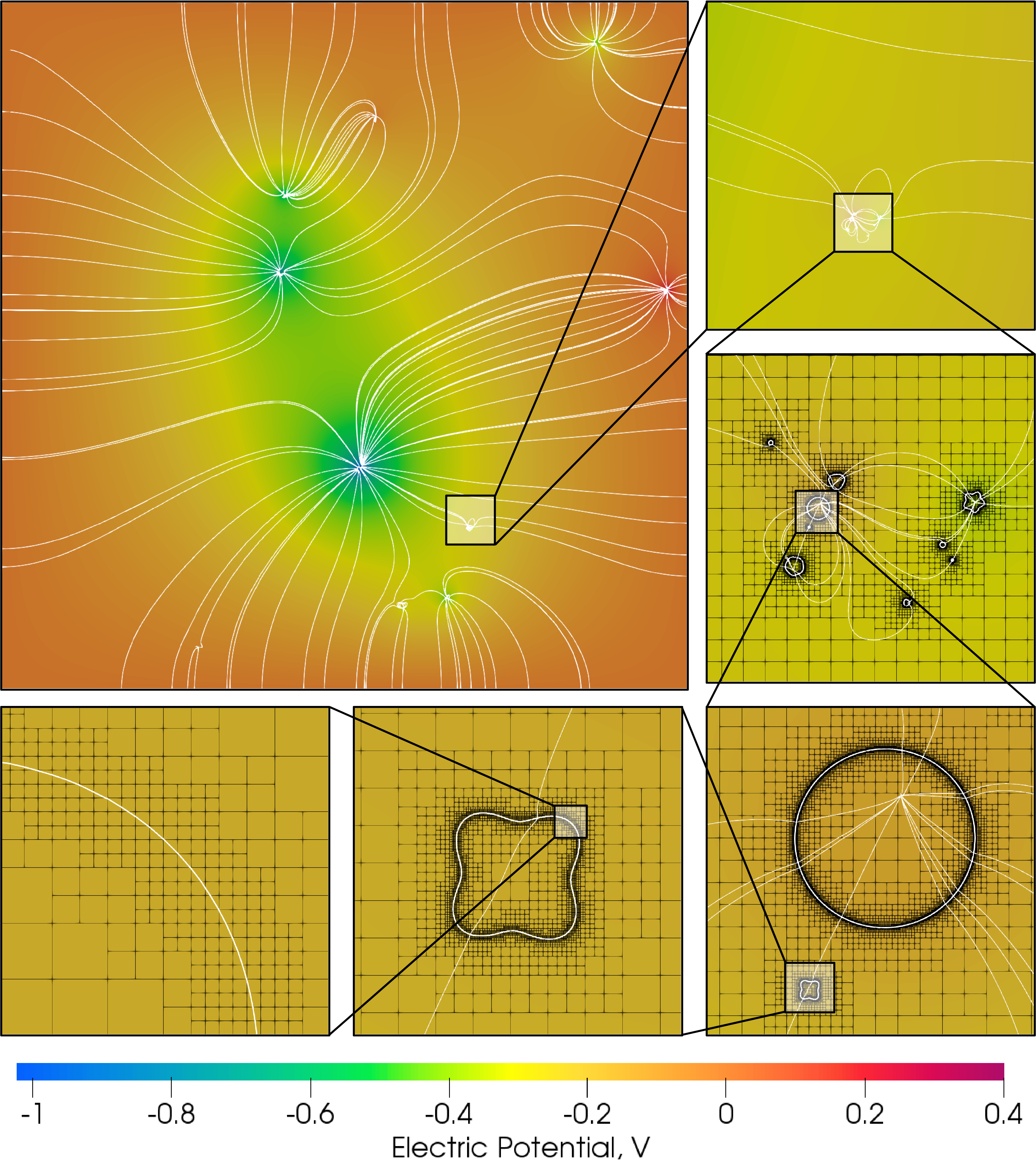
In this example, we consider 10 clusters of small star-shaped uniformly charged dielectric particles in a $2$m$\times$2m vacuum domain and compute the electric field generated by this configuration. The number of particles in each cluster varies from 3 to 10, the average size of clusters is 1 cm, particles have between 2 and 6 bumps and sizes in the range $[0.1;1]$ mm. The exact problem geometry description is provided in A. The absolute permittivity of particles is $10\varepsilon_{0}$ and their charge densities are $\pm 10^{5}\varepsilon_{0}$ (the sign is assigned to each particle randomly), where $\varepsilon_{0}$ is the vacuum permittivity. The domain boundaries are assumed to be a good conductor. Thus, the electric potential $\varphi\equiv u$ satisfies the boundary value problem (1)-(3) with parameters $k^{\pm}=\alpha=\beta=0$, $\mu^{-}=10$, $\mu^{+}=1$, $f^{-}=\pm 10^{5}$ (depending which particle is considered), $f^{+}=0$, $g=0$, where we denote the particles as $\Omega^{-}$ and the vacuum as $\Omega^{+}$.

Figure 9 depicts the electric potential $\phi$ and the electric field $\boldsymbol{E}=-\nabla\phi$ computed on an adaptive grid with the coarsest and finest mesh sizes corresponding to uniform resolutions of $2^{10}\times 2^{10}$ and $2^{20}\times 2^{20}$ grid points, respectively. Such a computational grid contains $2754021$ points, which is approximately just $0.00025\%$ of the total number of points in a uniform $2^{20}\times 2^{20}$ grid.

(a)

(b)

Figure 9: Application of the present method in the context of adaptive grids for computing electric field around clusters of charged dielectric particles: (a) The entire computational domain with successive zoom-ins for one of the clusters; (b) Zoom-ins for all other clusters. The color map indicates the electric potential and thin lines represent the electric field lines. The thicker white lines represent particles.

Remark: While the strategy of enforcing adaptive grids to be locally uniform around immersed interfaces is quite common and justified from the point of view of accuracy in many situations, it may not be very efficient for certain applications; in particular those where parts of the interface has high curvature while other parts are rather flat. However, it seems straightforward to adapt the described method to fully-adaptive (non-uniform along immersed interfaces) and Voronoi grids (including Voronoi partitions generated based on adaptive quadtree and octree grids). This will be considered in future works.

4 Conclusions

We have presented a simple finite volume numerical method for solving Elliptic equations with jump conditions across irregular interfaces that are implicitly represented by a level-set function on Cartesian grids. Second-order accurate solutions and first-order accurate gradients are obtained in the $L^{\infty}$-norm. The linear system is non-symmetric but the condition number is bounded, regardless of the ratio of the diffusion coefficients, so that the linear system can be inverted in a constant number of iterations that depends only on the grid resolution: the condition number scales as $\mathcal{O}\left(h^{-2}\right)$, similarly to the linear system obtained from the standard five-point stencil.

Future work will be focused on the analysis of the numerical scheme and its properties, the improvement to a superconvergent scheme (i.e, with second-order accurate gradients) and the extension to fully-adaptive (non-uniform along immersed interfaces) grids.

References

Appendix A Geometry description for adaptive grid example

The adaptive grid example (Section 3.4) deals with 67 particles each of which is described by a level-set function of the form:

$$\phi(r,\theta)=\sqrt{(r\cos(\theta-\theta_{0})-x_{c})^{2}+(r\sin(\theta-\theta_{0})-y_{c})^{2}}-r_{0}\left(1+\delta\cos(m(\theta-\theta_{0}))\right).$$

Parameters $x_{c}$, $y_{c}$, $r_{0}$, $\delta$, $m$ and $\theta_{0}$ for each particle as well as the sign of its charge are given in the following table:

Particle number	$x_{c}$	$y_{c}$	$r_{0}$	$\delta$	$m$	$\theta_{0}$	Charge
1	0.294320	-0.731980	0.000948	0.177428	5	3.779031	+
2	0.292603	-0.722570	0.000196	0.120466	2	0.575194	+
3	0.296621	-0.730048	0.000553	0.195375	3	5.983689	+
4	0.301392	-0.723932	0.000374	0.161709	3	1.178485	+
5	0.293268	-0.730192	0.000798	0.193548	3	6.112317	-
6	0.289541	-0.732616	0.000755	0.088156	4	2.266495	-
7	0.290527	-0.736414	0.000341	0.140005	3	6.140219	-
8	0.295213	-0.726113	0.000792	0.121836	5	0.884964	-
9	0.300884	-0.733236	0.000857	0.078646	4	1.588758	-
10	0.935243	0.156877	0.000462	0.026599	4	1.152778	+
11	0.936367	0.165333	0.000946	0.129853	3	2.585702	+
12	0.937713	0.161907	0.000114	0.111576	3	3.069164	+
13	0.927721	0.160662	0.000653	0.059185	4	4.986538	-
14	0.926407	0.164860	0.000243	0.009826	2	3.613796	-
15	0.939303	0.170991	0.000443	0.141560	3	2.988958	+
16	0.926755	0.162948	0.000482	0.025398	5	3.380732	+
17	0.936908	0.160965	0.000713	0.179751	3	0.252419	+
18	0.934454	0.162162	0.000448	0.011111	6	2.899990	+
19	0.160228	-0.743358	0.000329	0.052804	6	4.507911	+
20	0.164293	-0.747939	0.000792	0.015578	3	3.753404	+
21	0.173756	-0.744021	0.000264	0.186352	4	6.101247	+
22	0.168733	-0.761421	0.000999	0.001466	5	4.162976	-
23	0.170695	-0.747981	0.000389	0.025428	4	0.952773	-
24	0.160737	-0.760843	0.000209	0.199829	6	0.814897	-
25	0.725447	0.889409	0.000966	0.064583	3	5.719127	-
26	0.740474	0.893693	0.000453	0.004282	3	5.779404	-
27	0.736547	0.884784	0.000708	0.036598	4	0.871440	-
28	0.723810	0.875899	0.000367	0.044844	3	0.309913	-
29	0.742820	0.874970	0.000306	0.191154	4	1.616747	-
30	0.728138	0.878376	0.000857	0.026387	4	5.913726	-
31	0.728254	0.880038	0.000451	0.069948	6	2.499319	+
32	0.052907	-0.344586	0.000660	0.184134	4	2.412480	-
33	0.034801	-0.356601	0.000834	0.079140	4	4.794653	-
34	0.048034	-0.350902	0.000961	0.175580	4	1.000997	-
35	0.038434	-0.350375	0.000546	0.119999	5	5.330543	-
36	0.037001	-0.361473	0.000859	0.104759	6	2.104655	-
37	0.048676	-0.344655	0.000590	0.018488	3	3.979605	-
38	-0.182697	0.433937	0.000642	0.191264	5	0.196232	-
39	-0.180690	0.449481	0.000499	0.107538	4	3.958288	+
40	-0.171622	0.442325	0.000714	0.162207	3	4.889946	-
41	-0.177232	0.435290	0.000706	0.108419	6	2.765306	+
42	-0.182553	0.446933	0.000927	0.139933	5	0.682710	-
43	-0.169332	0.440621	0.000652	0.197255	6	0.524252	-
44	0.082096	0.665721	0.000309	0.018026	6	3.925875	+
45	0.070903	0.669204	0.000229	0.189876	3	1.973639	+
46	0.086667	0.652859	0.000256	0.009732	4	5.337312	-
47	0.089332	0.668903	0.000778	0.189929	4	0.506358	+
48	-0.416502	-0.873554	0.000168	0.038622	2	4.772787	+
49	-0.435866	-0.873537	0.000167	0.040327	6	4.357852	+
50	-0.428412	-0.875426	0.000329	0.067637	4	4.422504	-
51	0.367410	-0.528637	0.000239	0.004636	6	1.018504	-
52	0.364188	-0.533808	0.000271	0.072883	3	2.058938	-
53	0.357943	-0.522965	0.000682	0.097692	3	4.725618	+
54	0.354170	-0.530541	0.000809	0.035313	5	0.726723	-
55	0.355478	-0.527060	0.000107	0.166186	4	5.450653	+
56	0.356304	-0.525395	0.000985	0.004988	2	3.471888	+
57	0.368282	-0.530008	0.000107	0.133467	5	5.475823	-
58	0.370185	-0.524812	0.000830	0.145549	5	6.126808	-
59	0.352045	-0.519527	0.000198	0.011507	4	3.886958	+
60	-0.187080	0.207027	0.000928	0.121431	2	1.730282	+
61	-0.177875	0.213721	0.000126	0.001767	3	0.076936	+
62	-0.177947	0.216082	0.000647	0.130215	4	6.002824	-
63	-0.193546	0.211842	0.000749	0.088286	6	4.366932	-
64	-0.190933	0.205428	0.000170	0.122096	3	0.951230	-
65	-0.184008	0.210547	0.000752	0.030592	3	3.986605	-
66	-0.192313	0.214133	0.000925	0.029170	4	1.284015	-
67	-0.190761	0.223399	0.000728	0.195173	4	5.881409	-

References

- [1] L. Adams and T. Chartier. New geometric immersed interface multigrid solvers. SIAM J. of Scientific Comput, 25:1516–1533, 2004.
- [2] L. Adams and T. Chartier. A comparison of algebraic multigrid and geometric immersed interface multigrid methods for interface problems. SIAM J. of Scientific Comput, 26:762–784, 2005.
- [3] L. Adams and Z. Li. The immersed interface/multigrid methods for interface problems. SIAM J. of Scientific Comput, 24:202.
- [4] I. Babus̆ka. The finite element method for elliptic equations with discontinuous coefficients. Computing, 5:207–213, 1970.
- [5] S. Balay, J. Brown, K. Buschelman, W. D. Gropp, D. Kaushik, M. G. Knepley, L. C. McInnes, B. F. Smith, and H. Zhang. Petsc web page, 2012.
- [6] Z. Bao, J.-M. Hong, J. Teran, and R. Fedkiw. Fracturing rigid materials. IEEE Trans. on Vis. and Comput. Graph, 13:370–378, 2007.
- [7] T. Belytschko, N. Moës, S. Usui, and C. Parimi. Arbitrary discontinuities in finite elements. Int. J. for Num. Meth. Eng, 50:993–1013, 2001.
- [8] P. A. Berthelsen. A decomposed immersed interface method for variable coefficient elliptic equations with non-smooth and discontinuous solutions. Journal of Computational Physics, 197:364–386, 2004.
- [9] D. Bochkov and F. Gibou. A sharp computational method for the simulation of the solidification of multicomponent alloys. In Preparation, 2019.
- [10] D. Bochkov and F. Gibou. Solving poisson-type equations with robin boundary conditions on piecewise smooth interfaces. J. Comput. Phys., 376:1156–1198, 2019.
- [11] C. E. Brennen. Fundamentals of Multiphase Flows, volume ISBN 0521 848040. Cambridge University Press, 2005.
- [12] H. Chen, C. Min, and F. Gibou. A supra-convergent finite difference scheme for the Poisson and heat equations on irregular domains and non-graded adaptive Cartesian grids. J. Sci. Comput., 31:19–60, 2007.
- [13] T. Chen and J. Strain. Piecewise-polynomial discretization and krylov-accelerated multigrid for elliptic interface problems. Journal of Computational Physics, 227(16):7503–7542, 2008.
- [14] M. Cisternino and L. Weynans. A parallel second order cartesian method for elliptic interface problems. Commun. Comput. Phys., 12:1562–1587, 2012.
- [15] A. Coco and G. Russo. Second order multigrid methods for elliptic problems with discontinuous coefficients on an arbitrary interface, i: One dimensional problems. Numerical Mathematics: Theory, Methods & Applications, 5:19, 2012.
- [16] R. Crockett, P. Colella, and D. Graves. A cartesian grid embedded boundary method for solving the poisson and heat equations with discontinuous coefficients in three dimensions. J. Comput. Phys., 230(7):2451 – 2469, 2011.
- [17] C. Daux, N. Moës, J. Dolbow, N. Sukumar, and T. Belytschko. Arbitrary branched and intersecting cracks with the extended finite element method. Int. J. for Num. Meth. Eng, 48:1741–1760, 2000.
- [18] R. Egan and F. Gibou. Fast and scalable algorithms for constructing solvent-excluded surfaces of large biomolecules. Journal of Computational Physics, 374:91 – 120, 2018.
- [19] R. D. Falgout and U. M. Yang. Hypre: A library of high performance preconditioners, volume 2331. Springer Berlin Heidelberg, 2002.
- [20] R. Fedkiw, T. Aslam, B. Merriman, and S. Osher. A non-oscillatory eulerian approach to interfaces in multimaterial flows (the ghost fluid method). J. Comput. Phys., 152:457–492, 1999.
- [21] T. Fries and T. Belytschko. The intrinsic XFEM: a method for arbitrary discontinuities without additional unknowns. Int. J. for Num. Meth. in Eng, 68:1358–1385, 2006.
- [22] O. Gallinato and C. Poignard. Superconvergent Cartesian methods for Poisson type equations in 2d – domains. Technical report, 2015.
- [23] O. Gallinato and C. Poignard. Superconvergent second order cartesian method for solving free boundary problem for invadopodia formation. Journal of Computational Physics, 339:412 – 431, 2017.
- [24] O. Gallinato and C. Poignard. Superconvergent second order Cartesian method for solving free boundary problem for invadopodia formation. J. Comp. Phys., 339:412–431, 2017.
- [25] F. Gibou and R. Fedkiw. A fourth order accurate discretization for the Laplace and heat equations on arbitrary domains, with applications to the Stefan problem. J. Comput. Phys., 202(2):577 – 601, 2005.
- [26] F. Gibou, R. Fedkiw, L.-T. Cheng, and M. Kang. A second-order accurate symmetric discretization of the Poisson equation on irregular domains. J. Comput. Phys., 176:205–227, 2002.
- [27] F. Gibou, R. Fedkiw, and S. Osher. A review of level-set methods and some recent applications. Journal of Computational Physics, 353:82 – 109, 2018.
- [28] F. Gibou, C. Min, and R. Fedkiw. High resolution sharp computational methods for elliptic and parabolic problems in complex geometries. J. Sci. Comput., 54:369–413, 2013.
- [29] S. Groí and A. Reusken. An extended pressure finite element space for two-phase incompressible flows with surface tension. J. Comp. Phys, 224:40–58, 2007.
- [30] A. Guittet, M. Lepilliez, S. Tanguy, and F. Gibou. Solving elliptic problems with discontinuities on irregular domains – the Voronoi interface method. J. Comput. Phys., 298:747 – 765, 2015.
- [31] A. Guittet, C. Poignard, and F. Gibou. A voronoi interface approach to cell aggregate electropermeabilization. J. Comput. Phys., 332:143 – 159, 2017.
- [32] G. Guyomarc’h, C.-O. Lee, and K. Jeon. A discontinuous Galerkin method for elliptic interface problems with application to electroporation. Comm. Numer. Methods Engrg., 25(10):991–1008, 2009.
- [33] W.-F. Hu, M.-C. Lai, and Y.-N. Young. A hybrid immersed boundary and immersed interface method for electrohydrodynamic simulations. J. Comput. Phys., 282:47–61, 2015.
- [34] H. Ji and J. Dolbow. On strategies for enforcing interfacial constraints and evaluating jump conditions with extended finite element method. Int. J. for Num. Meth. in Eng, 61:204.
- [35] H. Johansen and P. Colella. A Cartesian grid embedded boundary method for Poisson equation on irregular domains. J. Comput. Phys., 147:60–85, 1998.
- [36] J. L. H. Jr., L. Wang, E. Sifakis, and J. M. Teran. A second order virtual node method for elliptic problems with interfaces and irregular domains in three dimensions. J. Comput. Phys., 231(4):2015 – 2048, 2012.
- [37] W. Kurz and D. J. Fisher. Fundamentals of Solidification. Trans Tech Publication, 1998.
- [38] A. J. Lew and G. C. Buscaglia. A discontinuous-Galerkin-based immersed boundary method. Int. J. for Num. Meth. in Eng, 76:427–454, 2008.
- [39] Z. Li. A fast iterative algorithm for elliptic interface problems. SIAM J. Numer. Anal., 35:230–254, 1998.
- [40] Z. Li and K. Ito. The Immersed Interface Method – Numerical Solutions of PDEs Involving Interfaces and Irregular Domains, volume 33. SIAM Frontiers in Applied mathematics, 2006.
- [41] X.-D. Liu, R. P. Fedkiw, and M. Kang. A boundary capturing method for Poisson’s equation on irregular domains. J. Comput. Phys., 160:151–178, 2000.
- [42] C. Min and F. Gibou. Geometric integration over irregular domains with application to level-set methods. J. Comput. Phys., 226:1432–1443, 2007.
- [43] C. Min and F. Gibou. A second order accurate level set method on non-graded adaptive Cartesian grids. J. Comput. Phys., 225(1):300–321, 2007.
- [44] M. Mirzadeh, M. Theillard, and F. Gibou. A second-order discretization of the nonlinear Poisson–Boltzmann equation over irregular geometries using non-graded adaptive Cartesian grids. J. Comput. Phys., 230(5):2125 – 2140, 2011.
- [45] M. Mirzadeh, M. Theillard, A. Helgadottir, D. Boy, and F. Gibou. An adaptive, finite difference solver for the nonlinear Poisson-Boltzmann equation with applications to biomolecular computations. Communications in Computational Physics, 13(1):150–173, 2012.
- [46] P. Mistani, A. Guittet, C. Poignard, and F. Gibou. A parallel voronoi-based approach for mesoscale simulations of cell aggregate electropermeabilization. Journal of Computational Physics, 380:48 – 64, 2019.
- [47] N. Moës, M. Cloirec, P. Cartraud, and J. Remacle. A computational approach to handle complex microstructure geometries. Comput. Methods Appl. Mech. Eng, 192:3162–3177, 2003.
- [48] N. Moës, J. Dolbow, and T. Belytschko. A finite element method for crack growth without remeshing. Int. J. for Num. Meth. Eng, 46:131–150, 1999.
- [49] N. Molino, J. Bao, and R. Fedkiw. A virtual node algorithm for changing mesh topology during simulation. ACM Trans. Graph. (SIGGRAPH Proc.), 23:385–392, 2004.
- [50] Y. T. Ng, H. Chen, C. Min, and F. Gibou. Guidelines for Poisson solvers on irregular domains with Dirichlet boundary conditions using the Ghost Fluid Method. Journal of Scientific Computing, 41(2):300–320, May 2009.
- [51] Y. T. Ng, C. Min, and F. Gibou. An efficient fluid–solid coupling algorithm for single-phase flows. J. Comput. Phys., 228(23):8807 – 8829, 2009.
- [52] M. Oevermann, C. Scharfenberg, and R. Klein. A sharp interface finite volume method for elliptic equations on Cartesian grids. J. Comp. Phys, 228:5184–5206, 2009.
- [53] S. Osher and R. Fedkiw. Level Set Methods and Dynamic Implicit Surfaces. Springer, 2003.
- [54] S. Osher and J. A. Sethian. Fronts propagating with curvature dependent speed: algorithms based on Hamilton-Jacobi formulations. J. Comput. Phys., 79(1):12–49, 1988.
- [55] J. Papac, F. Gibou, and C. Ratsch. Efficient symmetric discretization for the Poisson, heat and Stefan-type problems with Robin boundary conditions. J. Comput. Phys., 229:875–889, 2010.
- [56] C. Richardson, J. Hegemann, E. Sifakis, J. Hellrung, and J. Teran. An XFEM method for modeling geometrically elaborate crack propagation in brittle materials. Int. J. for Num. Meth. in Eng, 88:1042–1065, 2011.
- [57] P. Schwartz, M. Barad, P. Colella, and T. Ligocki. A Cartesian grid embedded boundary method for the heat equation and Poisson’s equation in three dimensions. J. Comp. Phys., 211(2):531–550, 2006.
- [58] J. A. Sethian. Level set methods, volume 3 of Cambridge Monographs on Applied and Computational Mathematics. Cambridge University Press, Cambridge, 1996. Evolving interfaces in geometry, fluid mechanics, computer vision, and materials science.
- [59] G. H. Shortley and R. Weller. Numerical solution of Laplace’s equation. J. Appl. Phys., 9:334–348, 1938.
- [60] E. Sifakis, K. Der, and R. Fedkiw. Arbitrary cutting of deformable tetrahedralized objects. In Proceedings of SIGGRAPH, 2007:73–80, 2007.
- [61] M. Theillard, F. Gibou, and T. Pollock. A sharp computational method for the simulation of the solidification of binary alloys. J. Sci. Comput., 63:330–354, 2014.
- [62] F. van der Bos and V. Gravemeier. Numerical simulation of premixed combustion using an enriched finite element method. J. Comp. Phys, 228:3605–3624, 2009.
- [63] A. Wiegmann and K. Bube. The explicit jump immersed interface method: finite difference method for pdes with piecewise smooth solutions. SIAM J. Numer. Anal., 37(3):827–862, 2000.
- [64] K. Xia, X. Feng, Z. Chen, Y. Tong, and G.-W. Wei. Multiscale geometric modeling of macromolecules i: Cartesian representation. Journal of Computational Physics, 257:912 – 936, 2014.
- [65] J.-J. Xu, W. Shi, W.-F. Hu, and J.-J. Huang. A level-set immersed interface method for simulating the electrohydrodynamics. J. Comput. Phys., 400:108956, 2020.
- [66] S. Xu. An iterative two-fluid pressure solver based on the immersed interface method. Communications in Computational Physics, 12(2):528–543, 2012.