Collaborative Quantization for Cross-Modal Similarity Search

Abstract

Cross-modal similarity search is a problem about designing a search system supporting querying across content modalities, e.g., using an image to search for texts or using a text to search for images. This paper presents a compact coding solution for efficient search, with a focus on the quantization approach which has already shown the superior performance over the hashing solutions in the single-modal similarity search. We propose a cross-modal quantization approach, which is among the early attempts to introduce quantization into cross-modal search. The major contribution lies in jointly learning the quantizers for both modalities through aligning the quantized representations for each pair of image and text belonging to a document. In addition, our approach simultaneously learns the common space for both modalities in which quantization is conducted to enable efficient and effective search using the Euclidean distance computed in the common space with fast distance table lookup. Experimental results compared with several competitive algorithms over three benchmark datasets demonstrate that the proposed approach achieves the state-of-the-art performance.

1 Introduction

Similarity search has been a fundamental problem in information retrieval and multimedia search. Classical approaches, however, are designed to address the single-modal search problem [25, 24, 27, 28, 13, 14], where, for instance, the text query is used to search in a text database, or the image query is used to search in an image database. In this paper, we deal with the cross-modal similarity search problem, which is an important problem emerged in multimedia information retrieval, for example, using a text query to retrieve images or using an image query to retrieve texts.

We study the compact coding solutions to cross-modal similarity search, in particular focusing on a common real-world scenario, image and text modalities. Compact coding is an approach of converting the database items into short codes on which similarity search can be efficiently conducted. It has been widely studied in single-modal similarity search with typical solutions including hashing [3, 15, 23] and quantization [5, 6, 16, 34, 26, 35], while relatively unexplored in cross-modal search except a few hashing approaches [1, 8, 11, 38]. We are interested in the quantization approach that represents each point by a short code formed by the index of the nearest center, as quantization has shown more powerful representation ability than hashing in single-modal search.

Rather than performing the quantization directly in the original feature space, we learn a common space for both modalities with the goal that the pair of image and text lie in the learnt common space closely. Learning such a common space is important and useful for the subsequent quantization whose similarity is computed based on the Euclidean distance. Similar observation has also been made in some hashing techniques [17, 18, 38] that apply the sign function on the learnt common space.

In this paper, we propose a novel approach for cross-modal similarity search, called collaborative quantization, that conducts the quantization simultaneously for both modalities in the common space, to which the database items of both modalities are mapped through matrix factorization. The quantization and the common space mapping are jointly optimized for both modalities under the objective that the quantized approximations of the descriptors of an image and a text forming a pair in the search database are well aligned. Our approach is one of the early attempts to introduce quantization into cross-modal similarity search offering the superior search performance. Experimental results on several standard datasets show that our approach outperforms existing cross-modal hashing and quantization algorithms.

2 Related work

Table 1: A brief categorization of the compact coding algorithms for cross-modal similarity search. The multi-modal relations are roughly divided into four categories: intra-modality (image vs. image and text vs. text), inter-modality (image vs. text), intra-document (correspondence of an image and a text forming a document, a special kind of inter-modality), and inter-document (document vs. document). Unified codes denote that the codes for an image and a text belonging to a document are the same, and separate codes denote that the codes are different.

Methods	Multi-modal data relations				Codes		Coding methods
	Intra-modality	Inter-modality	Intra-document	Inter-document	Unified	Separate	Hash	Quantization
CMSSH [1]		$\triangle$				$\triangle$	$\triangle$
SCM [32]		$\triangle$				$\triangle$	$\triangle$
CRH [36]		$\triangle$				$\triangle$	$\triangle$
MMNN [11]	$\triangle$	$\triangle$				$\triangle$	$\triangle$
$\textrm{SM}^{2}\textrm{H}$ [31]	$\triangle$	$\triangle$				$\triangle$	$\triangle$
MLBE [37]	$\triangle$	$\triangle$				$\triangle$	$\triangle$
IMH [20]	$\triangle$		$\triangle$			$\triangle$	$\triangle$
CVH [8]			$\triangle$	$\triangle$		$\triangle$	$\triangle$
MVSH [7]			$\triangle$	$\triangle$		$\triangle$	$\triangle$
SPH [9]			$\triangle$	$\triangle$	$\triangle$		$\triangle$
LSSH [38]			$\triangle$		$\triangle$		$\triangle$
CMFH [4]			$\triangle$		$\triangle$		$\triangle$
STMH [22]			$\triangle$		$\triangle$		$\triangle$
QCH [30]		$\triangle$				$\triangle$	$\triangle$
CCQ [10]			$\triangle$		$\triangle$			$\triangle$
Our approach			$\triangle$			$\triangle$		$\triangle$

There are two categories of compact coding approaches for cross-modal similarity search: cross-modal hashing and cross-modal quantization.

Cross-modal hashing often maps multi-modal data into a common Hamming space so that the hash codes of different modalities are directly comparable using the Hamming distance. After mapping, each document may have just one unified hash code, in which all the modalities of the document are mapped, or may have two separate hash codes, each corresponding to a modality. The main research problem in cross-modal hashing, besides hash function design that is also studied in single-modal search, is how to exploit and build the relations between the modalities. In general, the relations of multi-modal data, besides the intra-modality relation in the single modality (image vs. image and text vs. text) and the inter-modality relation across the modalities (image vs. text), also include intra-document (the correspondence of an image and a text forming a document, which is a special kind of inter-modality) and inter-document (document vs. document). A brief categorization is shown in Table 1.

The early approach, data fusion hashing [1], is a pairwise cross-modal similarity sensitive approach, which aligns the similarities (defined as inner product) in the Hamming space across the modalities, with the given inter-modality similar and dissimilar relations using the maximizing similarity-agreement criterion. An alternative formulation using the minimizing similarity-difference criterion is introduced in [32]. Co-regularized hashing [36] uses a smoothly clipped inverted squared deviation function to connect the inter-modality relation with the similarity over the projections that form the hashing codes. Similar regularization techniques are adopted for multi-modal hashing in [12]. In addition to the inter-modality similarities, several other hashing techniques, such as multimodal similarity-preserving hashing [11], sparse hashing approach [31], a probabilistic model for hashing [37], also explore and utilize the intra-modality relation to learn the hash codes for each modality.

Cross-view hashing [8] defines the distance between documents in the Hamming space by considering the hash codes of all the modalities, and aligns it with the given inter-document similarity. Multi-view spectral hashing [7] adopts a similar formulation but with a different optimization algorithm. These methods usually also involve the intra-document relation in an implicit way by considering the multi-modal document as an integrated whole object. There are other hashing methods exploring the inter-document relation about multi-modal representation , but not for cross-modal similarity search, such as composite hashing [33] and effective multiple feature hashing [19].

The intra-document relation is often used to learn a unified hash code, into which a hash function is learnt for each modality to map the feature. For example, Latent semantic sparse hashing [38] applies the sign function on the joint space projected from the latent semantic representation learnt for each modality. Collective matrix factorization hashing [4] finds the common (same) representation for an image-text pair via collective matrix factorization, and obtains the hash codes directly using the sign function on the common representation. Other methods exploring the intra-document relation include semantic topic multimodal hashing [22], semantics-preserving multi-view hashing [9], inter-media hashing [33] and its accelerated version [39], and so on. Meanwhile, several attempts [29, 21] have been made based on the neural network which can also be combined with our approach to learn the common space.

Recently, a few techniques based on quantization are developed for cross-modal search. Quantized correlation hashing [30] combines the hash function learning with the quantization by minimizing the inter-modality similarity disagreement as well as the binary quantization simultaneously. Compositional correlation quantization [10] projects the multi-modal data into a common space, and then obtains a unified quantization representation for each document. Our approach, also exploring the intra-document relation, belongs to this cross-modal quantization category and achieves the state-of-the-art performance.

3 Formulation

We study the similarity search problem over a database $\mathcal{Z}$ of documents with two modalities: image and text. Each document is a pair of image and text, $\mathcal{Z}=\{(\mathbf{x}_{n},\mathbf{y}_{n})\}_{n=1}^{N}$, where $\mathbf{x}_{n}\in\mathbb{R}^{D_{I}}$ is a $D_{I}$-dimensional feature vector describing an image, and $\mathbf{y}_{n}\in\mathbb{R}^{D_{T}}$ is a $D_{T}$-dimensional feature vector describing a text. Splitting the database $\mathcal{Z}$ yields two databases each formed by images and texts separately, i.e., $\mathcal{X}=\{\mathbf{x}_{1},\mathbf{x}_{2},\cdots,\mathbf{x}_{N}\}$ and $\mathcal{Y}=\{\mathbf{y}_{1},\mathbf{y}_{2},\cdots,\mathbf{y}_{N}\}$. Given a image (text) query $\mathbf{x}_{q}$ ($\mathbf{y}_{q}$), the goal of cross-modality similarity search is to retrieve the closest match in the text (image) database: $\arg\max_{\mathbf{y}\in\mathcal{Y}}\operatorname{sim}(\mathbf{x}_{q},\mathbf{y})$ ($\arg\max_{\mathbf{x}\in\mathcal{X}}\operatorname{sim}(\mathbf{y}_{q},\mathbf{x})$).

Rather than directly quantizing the feature vectors $\mathbf{x}$ and $\mathbf{y}$ to $\bar{\mathbf{x}}$ and $\bar{\mathbf{y}}$, which requires a further non-trivial scheme to learn the similarity for vectors $\bar{\mathbf{x}}$ and $\bar{\mathbf{y}}$ with different dimensions, we are interested in finding the common space for both image and text, and jointly quantizing the image and text descriptors in the common space, so that the Euclidean distance which is widely-used in single-modal similarity search, can also be used for the cross-modal similarity evaluation.

Collaborative quantization. Suppose the images and the texts in the $D$-dimensional common space are represented as $\mathbf{X}^{\prime}=[\mathbf{x}^{\prime}_{1},\mathbf{x}^{\prime}_{2},\cdots,\mathbf{x}^{\prime}_{N}]$ and $\mathbf{Y}^{\prime}=[\mathbf{y}^{\prime}_{1},\mathbf{y}^{\prime}_{2},\cdots,\mathbf{y}^{\prime}_{N}]$. For each modality, we propose to adopt composite quantization [34] to quantize the vectors in the common space. Composite quantization aims to approximate the images $\mathbf{X}^{\prime}$ as $\mathbf{X}^{\prime}\approx\bar{\mathbf{X}}=\mathbf{C}\mathbf{P}$ by minimizing

$$\|\mathbf{X}^{\prime}-\mathbf{C}\mathbf{P}\|_{F}^{2}.$$ (1)

Here, $\mathbf{C}=[\mathbf{C}_{1},\mathbf{C}_{2},\cdots,\mathbf{C}_{M}]$ corresponds to the $M$ dictionaries, $\mathbf{C}_{m}=[\mathbf{c}_{m1},\mathbf{c}_{m2},\cdots,\mathbf{c}_{mK}]$ corresponds to the $m$th dictionary of size $K$ and each column is a dictionary element. $\mathbf{P}=[\mathbf{p}_{1},\mathbf{p}_{2},\cdots,\mathbf{p}_{N}]$ with $\mathbf{p}_{n}=[\mathbf{p}_{n1}^{T},\mathbf{p}_{n2}^{T},\cdots,\mathbf{p}_{nm}^{T}]^{T}$, and $\mathbf{p}_{nm}$ is a $K$-dimensional binary ($0$,$1$) vector with only $1$-valued entry indicating that the corresponding element in the $m$th dictionary is selected to compose $\mathbf{x}^{\prime}_{n}$. The texts $\mathbf{Y}^{\prime}$ in the common space are approximated as $\mathbf{Y}^{\prime}\approx\bar{\mathbf{Y}}=\mathbf{D}\mathbf{Q}$, and the meaning of the symbols is similar to that in the images.

Besides the quantization quality, we explore the intra-document correlation between images and texts for the quantization: the image and the text forming a document are close after quantization, which is the bridge to connect images and texts for cross-modal search. We adopt the following simple formulation that minimizes the distance between the image and the corresponding text,

$$\|\mathbf{C}\mathbf{P}-\mathbf{D}\mathbf{Q}\|_{F}^{2}.$$ (2)

The overall collaborative quantization formulation is given as follows,

$$\mathcal{Q}(\mathbf{C},\mathbf{P};\mathbf{D},\mathbf{Q})=$$ (3)

$$\|\mathbf{X}^{\prime}-\mathbf{C}\mathbf{P}\|^{2}_{F}+\|\mathbf{Y}^{\prime}-\mathbf{D}\mathbf{Q}\|^{2}_{F}+\gamma\|\mathbf{C}\mathbf{P}-\mathbf{D}\mathbf{Q}\|^{2}_{F},$$

where $\gamma$ is a trade-off variable to balance the quantization quality and the correlation degree.

Common space mapping. The common space mapping problem aims to map the data in different modalities into the same space so that the representations in cross-modalities are comparable. In our problem, we want to map the $N$ $D_{I}$-dimensional image data $\mathbf{X}$ and the $N$ $D_{T}$-dimensional text data $\mathbf{Y}$ to the same $D$-dimensional data: $\mathbf{X}^{\prime}$ and $\mathbf{Y}^{\prime}$.

We choose the matrix-decomposition solution as in [38]: the image data $\mathbf{X}$ is approximated using sparse coding as a product of two matrices $\mathbf{B}\mathbf{S}$, and the sparse code $\mathbf{S}$ is shown to be a good representation of the raw feature $\mathbf{X}$; the text data $\mathbf{Y}$ is also decomposed into two matrices, $\mathbf{U}$ and $\mathbf{Y}^{\prime}$, where $\mathbf{Y}^{\prime}$ is the low-dimensional representation; In addition, a transformation matrix $\mathbf{R}$ is introduced to align the image sparse code $\mathbf{S}$ with the text code $\mathbf{Y}^{\prime}$ by minimizing $\|\mathbf{Y}^{\prime}-\mathbf{R}\mathbf{S}\|_{F}^{2}$, and the image in the common space is represented as $\mathbf{X}^{\prime}=\mathbf{R}\mathbf{S}$. The objective function for common space mapping is written as follows,

$$\mathcal{M}(\mathbf{B},\mathbf{S};\mathbf{U},\mathbf{Y}^{\prime};\mathbf{R})=$$ (4)

$$\|\mathbf{X}-\mathbf{B}\mathbf{S}\|^{2}_{F}+\rho|\mathbf{S}|_{11}+\eta\|\mathbf{Y}-\mathbf{U}\mathbf{Y}^{\prime}\|^{2}_{F}+\lambda\|\mathbf{Y}^{\prime}-\mathbf{R}\mathbf{S}\|^{2}_{F}.$$

Here $|\mathbf{S}|_{11}=\sum_{i=1}^{N}\|\mathbf{S}_{\cdot i}\|_{1}$ is the sparse term, and $\rho$ determines the sparsity degree; $\eta$ is used to balance the scales of image and text representations; $\lambda$ is a trade-off parameter to control the approximation degree in each modality and the alignment degree for the pair of image and text.

Overall objective function. In summary, the overall formulation of the proposed cross-modal quantization is,

$$\min~ ~\mathcal{F}(\boldsymbol{\theta}_{q},\boldsymbol{\theta}_{m})=\mathcal{Q}(\mathbf{C},\mathbf{P};\mathbf{D},\mathbf{Q})+\mathcal{M}(\mathbf{B},\mathbf{S};\mathbf{U},\mathbf{Y}^{\prime};\mathbf{R})$$

$$\operatorname{s.t.}~ ~\|\mathbf{B}_{\cdot i}\|_{2}^{2}\leqslant 1,\|\mathbf{U}_{\cdot i}\|_{2}^{2}\leqslant 1,\|\mathbf{R}_{\cdot i}\|_{2}^{2}\leqslant 1,$$ (5)

$$~\sum\nolimits_{i=1}^{M}\sum\nolimits_{j=1,j\neq i}^{M}\mathbf{p}_{ni}^{T}\mathbf{C}_{i}^{T}\mathbf{C}_{j}\mathbf{p}_{nj}=\epsilon_{1},$$ (6)

$$~\sum\nolimits_{i=1}^{M}\sum\nolimits_{j=1,j\neq i}^{M}\mathbf{q}_{ni}^{T}\mathbf{D}_{i}^{T}\mathbf{D}_{j}\mathbf{q}_{nj}=\epsilon_{2},$$ (7)

where $\boldsymbol{\theta}_{q}$ and $\boldsymbol{\theta}_{m}$ represent the parameters in quantization and mapping, i.e., $(\mathbf{C},\mathbf{P};\mathbf{D},\mathbf{Q})$ and $(\mathbf{B},\mathbf{S};\mathbf{U},\mathbf{Y}^{\prime};\mathbf{R})$ respectively. The constraints in Equation 6 and Equation 7 are introduced for fast distance computation as in composite quantization [34], and more details about the search process are presented in Section 4.3.

4 Optimization

We optimize the Problem 5 by alternatively solving two sub-problems: common space mapping with the quantization parameters fixed: $\min\mathcal{F}(\boldsymbol{\theta}_{m}|\boldsymbol{\theta}_{q})=\mathcal{M}(\boldsymbol{\theta}_{m})+\|\mathbf{X}^{\prime}-\mathbf{C}\mathbf{P}\|^{2}_{F}+\|\mathbf{Y}^{\prime}-\mathbf{D}\mathbf{Q}\|^{2}_{F}$, and collaborative quantization with the mapping parameters fixed: $\min\mathcal{F}(\boldsymbol{\theta}_{q}|\boldsymbol{\theta}_{m})=\min\mathcal{Q}(\boldsymbol{\theta}_{q})$. Each of the two sub-problems is solved again by a standard iteratively alternative algorithm.

4.1 Common space mapping

The objective function of the common space mapping with the quantization parameters fixed is,

$$\min_{\boldsymbol{\theta}_{m}}~ \mathcal{M}(\boldsymbol{\theta}_{m})+\|\mathbf{X}^{\prime}-\mathbf{C}\mathbf{P}\|^{2}_{F}+\|\mathbf{Y}^{\prime}-\mathbf{D}\mathbf{Q}\|^{2}_{F}$$ (8)

$$\operatorname{s.t.}~ ~\|\mathbf{B}_{\cdot i}\|_{2}^{2}\leqslant 1,\|\mathbf{U}_{\cdot i}\|_{2}^{2}\leqslant 1,\|\mathbf{R}_{\cdot i}\|_{2}^{2}\leqslant 1.$$ (9)

The iteration details are given below.

Update $\mathbf{Y}^{\prime}$. The objective function with respect to $\mathbf{Y}^{\prime}$ is an unconstrained quadratic optimization problem, and is solved by the following closed-form solution,

$$\mathbf{Y}^{\prime*}=(\eta\mathbf{U}^{T}\mathbf{U}+(\lambda+1)\mathbf{I})^{-1}(\mathbf{D}\mathbf{Q}+\eta\mathbf{U}^{T}\mathbf{Y}+\lambda\mathbf{R}\mathbf{S}),$$

where $\mathbf{I}$ is the identity matrix.

Update $\mathbf{S}$. The objective function with respect to $\mathbf{S}$ can be transformed to,

$$\small\min_{\mathbf{S}}~ \|\left[\begin{array}[]{c}\sqrt{\frac{1}{\lambda+1}}\mathbf{X}\\ \frac{1}{\lambda+1}(\mathbf{CP}+\lambda\mathbf{A})\end{array}\right]-\left[\begin{array}[]{c}\sqrt{\frac{1}{\lambda+1}}\mathbf{B}\\ \mathbf{R}\end{array}\right]\mathbf{S}\|_{F}^{2}$$

$$+\frac{\rho}{\lambda+1}|\mathbf{S}|_{11},$$ (14)

which is solved using the sparse learning with efficient projections package.

Update $\mathbf{U,B,R}$. The algorithms for updating $\mathbf{U,B,R}$ are the same, as we can see from the following formulas,

$$\min_{\mathbf{U}}~ \|\mathbf{Y}-\mathbf{U}\mathbf{Y}^{\prime}\|^{2}_{F},~~\operatorname{s.t.}~\|\mathbf{U}_{\cdot i}\|_{2}^{2}\leqslant 1,$$ (15)

$$\min_{\mathbf{B}}~ \|\mathbf{X}-\mathbf{B}\mathbf{S}\|^{2}_{F},~~\operatorname{s.t.}~\|\mathbf{B}_{\cdot i}\|_{2}^{2}\leqslant 1,$$ (16)

$$\min_{\mathbf{R}}~ \|\frac{1}{\lambda+1}(\mathbf{CP}+\lambda\mathbf{Y}^{\prime})-\mathbf{RS}\|^{2}_{F},~~\operatorname{s.t.}~\|\mathbf{R}_{\cdot i}\|_{2}^{2}\leqslant 1.$$

All of the above three learning problems are minimizing the quadratically constrained least square problem, which has been well studied in numerical optimization field and can be readily solved using the primal-dual conjugate gradient method.

4.2 Collaborative quantization

The second sub-problem is transformed to an unconstrained formulation by adding the equality constraints as a penalty regularization with a penalty parameter $\mu$,

$$\Psi=\mathcal{Q}(\boldsymbol{\theta}_{q})+\mu\sum\nolimits_{n=1}^{N}(\sum\nolimits_{i\neq j}^{M}\mathbf{p}_{ni}^{T}\mathbf{C}_{i}^{T}\mathbf{C}_{j}\mathbf{p}_{nj}-\epsilon_{1})^{2}$$

$$+\mu\sum\nolimits_{n=1}^{N}(\sum\nolimits_{i\neq j}^{M}\mathbf{q}_{ni}^{T}\mathbf{D}_{i}^{T}\mathbf{D}_{j}\mathbf{q}_{nj}-\epsilon_{2})^{2},$$ (17)

which is solved by alternatively updating each variable with others fixed.

Update $\mathbf{C}$ ($\mathbf{D}$). The optimization procedures for $\mathbf{C}$ and $\mathbf{D}$ are essentially the same, so we only show how to optimize $\mathbf{C}$. We adopt the L-BFGS algorithm, one of the most frequently-used quasi-Newton methods, to solve the unconstrained non-linear problem with respect to $\mathbf{C}$. The derivative of the objective function is $[\frac{\partial\Psi}{\mathbf{C}_{1}},\cdots,\frac{\partial\Psi}{\mathbf{C}_{M}}]$,

$$\frac{\partial\Psi}{\partial\mathbf{C}_{m}}=2((\gamma+1)\mathbf{CP}-\mathbf{RS}-\gamma\mathbf{DQ})\mathbf{P}_{m}^{T}$$ (18)

$$+ \sum\limits_{n=1}^{N}[4\mu(\sum\limits_{i\neq j}^{M}\mathbf{p}_{ni}^{T}\mathbf{C}_{i}^{T}\mathbf{C}_{j}\mathbf{p}_{nj}-\epsilon_{1})(\sum\limits_{l=1,l\neq m}^{M}\mathbf{C}_{l}\mathbf{p}_{nl})\mathbf{p}_{nm}^{T}],$$

where $\mathbf{P}_{m}=[\mathbf{p}_{1m},\cdots,\mathbf{p}_{Nm}]$.

Update $\epsilon_{1},\epsilon_{2}$. With other variables fixed, it is easy to get the optimal solution,

$$\epsilon_{1}^{*}=\frac{1}{N}\sum\nolimits_{n=1}^{N}\sum\nolimits_{i\neq j}^{M}\mathbf{p}_{ni}^{T}\mathbf{C}_{i}^{T}\mathbf{C}_{j}\mathbf{p}_{nj},$$ (19)

$$\epsilon_{2}^{*}=\frac{1}{N}\sum\nolimits_{n=1}^{N}\sum\nolimits_{i\neq j}^{M}\mathbf{q}_{ni}^{T}\mathbf{D}_{i}^{T}\mathbf{D}_{j}\mathbf{q}_{nj}.$$ (20)

Update $\mathbf{P}$ ($\mathbf{Q}$). The binary vectors $\{\mathbf{p}_{n}\}_{n=1}^{N}$ given other variables fixed are independent with each other, and hence the optimization problem can be decomposed into $N$ sub-problems,

$$\Psi_{n}=~ \|\mathbf{x}^{\prime}_{n}-\mathbf{C}\mathbf{p}_{n}\|_{2}^{2}+\gamma\|\mathbf{C}\mathbf{p}_{n}-\mathbf{D}\mathbf{q}_{n}\|_{2}^{2}$$ (21)

$$+~ \mu(\sum\nolimits_{i\neq j}^{M}\mathbf{p}_{ni}^{T}\mathbf{C}_{i}^{T}\mathbf{C}_{j}\mathbf{p}_{nj}-\epsilon_{1})^{2}.$$ (22)

This problem is a mixed-binary-integer problem generally considered as NP-hard. As a result, we approximately solve this problem by greedily updating the $M$ indicating vectors $\{\mathbf{p}_{nm}\}_{m=1}^{M}$ in cycle: fixing $\{\mathbf{p}_{nm^{\prime}}\}_{m^{\prime}=1,m^{\prime}\neq m}^{M}$, $\mathbf{p}_{nm}$ is updated by exhaustively checking all the elements in $\mathbf{C}_{m}$, finding the element such that the objective function is minimized, and setting the corresponding entry of $\mathbf{p}_{nm}$ to be 1 and all the others to be 0. Similar optimization procedure is adopted to update $\mathbf{Q}$.

4.3 Search process

In cross-modal search, the given query can be either an image or a text, which require different querying processes.

Image query. If the query is an image, $\mathbf{x}_{q}$, we first obtain the representation in the common space, $\mathbf{x}_{q}^{\prime}=\mathbf{Rs}^{*}$,

$$\mathbf{s}^{*}=\text{arg}\min_{\mathbf{s}}~ \|\mathbf{x}_{q}-\mathbf{B}\mathbf{s}\|^{2}_{2}+\rho|\mathbf{s}|_{1}.$$ (23)

The approximated distance between the image query $\mathbf{x}_{q}$ and the database text $\mathbf{y}_{n}$ (represented as $\mathbf{Dq}_{n}=\sum_{m=1}^{M}\mathbf{D}_{m}\mathbf{q}_{nm}$) is,

$$\|\mathbf{x}_{q}^{\prime}-\mathbf{Dq}_{n}\|_{2}^{2}=\sum\nolimits_{m=1}^{M}\|\mathbf{x}_{q}^{\prime}-\mathbf{D}_{m}\mathbf{q}_{nm}\|_{2}^{2}$$ (24)

$$-(M-1)\|\mathbf{x}_{q}^{\prime}\|_{2}^{2}+\sum\nolimits_{i\neq j}^{M}\mathbf{q}_{ni}^{T}\mathbf{D}_{i}^{T}\mathbf{D}_{j}\mathbf{q}_{nj}.$$ (25)

The last term $\sum\nolimits_{i\neq j}^{M}\mathbf{q}_{ni}^{T}\mathbf{D}_{i}^{T}\mathbf{D}_{j}\mathbf{q}_{nj}$ is constant for all the texts due to the introduced equality constraint in Equation 7. Hence given $\mathbf{x}_{q}^{\prime}$, it is enough to compute the first term $\sum\nolimits_{m=1}^{M}\|\mathbf{x}_{q}^{\prime}-\mathbf{D}_{m}\mathbf{q}_{nm}\|_{2}^{2}$ to search for the nearest neighbors, which furthermore can be efficiently computed and takes $O(M)$ by looking up a precomputed distance table storing the distances: $\{\|\mathbf{x}_{q}^{\prime}-\mathbf{d}_{mk}\|_{2}^{2}~|~m=1,\cdots,M;k=1,\cdots,K\}$.

Text query. When the query comes as a text, $\mathbf{y}_{q}$, the representation $\mathbf{y}_{q}^{\prime}$ is obtained by solving,

$$\mathbf{y}_{q}^{\prime}=\text{arg}\min_{\mathbf{y}}~ \|\mathbf{y}_{q}-\mathbf{U}\mathbf{y}\|^{2}_{2}.$$ (26)

Using $\mathbf{y}_{q}^{\prime}$ to search in the image database is similar to that in the image query search process.

5 Discussions

Relation to compositional correlation quantization. The proposed approach is close to compositional correlation quantization [10], which is also a quantization-based method for cross-modal search. In fact, our approach differs from it in two ways: (1) we find a different mapping function to project the common space; (2) we learn separate quantized centers for a pair using two dictionaries instead of the unified quantized centers in compositional correlation quantization [10] imposed with a harder alignment using one dictionary. Hence, during the quantization stage, our approach can obtain potentially smaller quantization error, as the quantized center is more flexible, and thus produce better search performance. The empirical comparison illustrating the effect of dictionary is shown in Figure 2.

Relation to latent semantic sparse hashing. In our formulation, the common space is learnt in a similar manner with latent semantic sparse hashing [38]. After the common space mapping, latent semantic sparse hashing applies a simple sign function directly on the common space, which can result in large information loss and hence weaken the search performance. Our approach, however, adopts the quantization technique that has more accurate distance approximation than hashing, and produces better cross-modal search quality than latent semantic sparse hashing, which is verified in our experiments shown in Table 2 and Figure 3.

Table 2: MAP$@50$ comparison of different algorithms on all the benchmark datasets under various code lengths. We also report the results of CMFH and CCQ (whose code implementations are not publicly available) in their corresponding papers and we distinguish those results by parenthesis $()$. “——” is used in the place where the result under that specific setting is not reported in their papers. Different setting refers to different datasets, or (and) different features, or (and) different bits, and so on.

Task	Method	Wiki				FLICKR$25K$				NUS-WIDE
		16 bits	32 bits	64 bits	128 bits	16 bits	32 bits	64 bits	128 bits	16 bits	32 bits	64 bits	128 bits
Img to Txt	CMSSH [1]	0.2110	0.2115	0.1932	0.1909	0.6468	0.6616	0.6681	0.6624	0.5243	0.5210	0.5211	0.4813
	CVH [8]	0.1947	0.1798	0.1732	0.1912	0.6450	0.6363	0.6273	0.6204	0.5352	0.5254	0.5011	0.4705
	MLBE [37]	0.3537	0.3947	0.2599	0.2247	0.6085	0.5866	0.5841	0.5883	0.4472	0.4540	0.4703	0.4026
	QCH [30]	0.1490	0.1726	0.1621	0.1611	0.5722	0.5780	0.5618	0.5567	0.5090	0.5270	0.5208	0.5135
	LSSH [38]	0.2396	0.2336	0.2405	0.2373	0.6328	0.6403	0.6451	0.6511	0.5368	0.5527	0.5674	0.5723
	CMFH [4]	0.2548	0.2591	0.2594	0.2651	0.5886	0.6067	0.6343	0.6550	0.4740	0.4821	0.5130	0.5068
	(CMFH [4])	(0.2538)	(0.2582)	(0.2619)	(0.2648)	——	——	——	——	——	——	——	——
	(CCQ [10])	(0.2513)	(0.2529)	(0.2587)	——	——	——	——	——	——	——	——	——
	CMCQ	0.2478	0.2513	0.2567	0.2614	0.6705	0.6716	0.6782	0.6821	0.5637	0.5902	0.5990	0.6096
Txt to Img	CMSSH [1]	0.2446	0.2505	0.2387	0.2352	0.6123	0.6400	0.6382	0.6242	0.4177	0.4259	0.4187	0.4203
	CVH [8]	0.3186	0.2354	0.2046	0.2085	0.6595	0.6507	0.6463	0.6580	0.5601	0.5439	0.5160	0.4821
	MLBE [37]	0.3336	0.3993	0.4897	0.2997	0.5937	0.6182	0.6550	0.6392	0.4352	0.4888	0.5020	0.4425
	QCH [30]	0.1924	0.1561	0.1800	0.1917	0.5752	0.6002	0.5757	0.5723	0.5099	0.5172	0.5092	0.5089
	LSSH [38]	0.5776	0.5886	0.5998	0.6103	0.6504	0.6726	0.6965	0.7010	0.6357	0.6638	0.6820	0.6926
	CMFH [4]	0.6153	0.6363	0.6411	0.6504	0.5873	0.6019	0.6477	0.6623	0.5109	0.5643	0.5896	0.5943
	(CMFH [4])	(0.6116)	(0.6298)	(0.6398)	(0.6477)	——	——	——	——	——	——	——	——
	(CCQ [10])	(0.6351)	(0.6394)	(0.6405)	——	——	——	——	——	——	——	——	——
	CMCQ	0.6397	0.6474	0.6546	0.6593	0.7248	0.7335	0.7394	0.7550	0.6898	0.7086	0.7194	0.7254

6 Experiments

6.1 Setup

Datasets. We evaluate our method on three benchmark datasets. The first dataset, Wiki consists of 2,866 images and 2,866 texts describing the images in short paragraph (at least 70 words), with images represented as 128-dimensional SIFT features and texts expressed as 10-dimensional topics vectors. This dataset is divided into 2,173 image-text pairs and 693 quries, and each pair is labeled with one of the 10 semantic classes. The second dataset, FLICKR25K, is composed of 25,000 images along with the user assigned tags. The average number of tags for an image is 5.15 [21]. Each image-text pair is assigned with multiple labels from a total of 38 classes. As in [21], the images are represented by 3857-dimensional features and the texts are 2000-dimensional vectors indicating the occurrence of the tags. We randomly sampled $10\%$ of the pairs as the test set and use the remaining as the training set. The third dataset is NUS-WIDE [2] containing 269,648 images with associated tags (6 in average), each pair is annotated with multiple labels among 81 concepts. As done in previous work [4, 36, 38], we select 10 most popular concepts resulting in 186,577 data pairs. The images are represented by 500-dimensional bag-of-words features based on SIFT descriptors, and the texts are 1000-dimensional vectors of the most frequent tags. Following [38], We use 4000 ($\approx 2\%$) randomly sampled pairs as the query set and the rest as the training set.

Evaluation. In our experiments, we report the results of two search tasks for the cross-modal search, i.e., the image (as the query) to text (as the database) task and the text to image task. The search quality is evaluated with two measures: MAP$@T$ and precision$@T$. MAP$@T$ is defined as the mean of the average precisions of all the queries, and the average precision of a query is computed as, $AP(\mathbf{q})=\frac{\sum_{t=1}^{T}P_{\mathbf{q}}(t)\delta(t)}{\sum_{t=1}^{T}\delta(t)}$, where $T$ is the number of retrieved items, $P_{\mathbf{q}}(t)$ is the precision at position $t$ for query $\mathbf{q}$, and $\delta(t)=1$ if the retrieved $t$th item has the same label with query $\mathbf{q}$ or shares at least one label, otherwise $\delta(t)=0$. Following [38, 4, 10], we report MAP$@T$ with $T=50$ and $T=100$. We also plot the precision$@T$ curve which is obtained by computing the precisions at different recall levels through varying the number of retrieved items.

Compared methods. We compare our approach, Cross-Modal Collaborative Quantization (CMCQ), with three baseline methods that only use the intra-document relation: Latent Semantic Sparse Hashing (LSSH) [38], Collective Matrix Factorization Hashing (CMFH) [4], and Compositional Correlation Quantization (CCQ) [10]. The code of LSSH is generously provided by the authors and we implemented the CMFH carefully by ourselves. The performance of CCQ (without public code) is presented partially using the results in its paper. In addition, we report the state-of-the-art algorithms whose codes are publicly available: (1) Cross-Modal Similarity Sensitive Hashing (CMSSH) [1], (2) Cross-View Hashing (CVH) [8], (3) Multimodal Latent Binary Embedding (MLBE) [37], (4) Quantized Correlation Hashing (QCH) [30]. The parameters in above methods are set according to the corresponding papers.

Implementation details. The data for both modalities are mean-centered and then normalized to have unit Euclidean length. We use principle component analysis to project the image into a lower dimensional (set to 64) space, and the number of bases in sparse coding is set to 512 ($\mathbf{B}\in\mathbb{R}^{64\times 512}$). The latent dimension of matrix factorization for text data is set equal to the number of code bits, e.g., 16, 32 etc. The mapping parameters (denoted as $\boldsymbol{\theta}_{m}$) are initialized by solving a relatively easy problem $\min\mathcal{M}(\boldsymbol{\theta}_{m})$ (similar algorithm with that presented in solving $\min\mathcal{F}(\boldsymbol{\theta}_{m}|\boldsymbol{\theta}_{q})$). Then the quantization parameters (denoted as $\boldsymbol{\theta}_{q}$) are initialized by conducting composite quantization [34] in the common space.

There are five parameters balancing different trade-offs in our algorithm: the sparsity degree $\rho$, the scale-balance parameter $\eta$, the alignment degree in the common space $\lambda$, the correlation degree of the quantization $\gamma$, and the penalty parameter $\mu$. We simply set $\mu=0.1$ in our experiments as it has already shown satisfactory results. The other four parameters are selected through validation (by varying one parameter in $\{0.1,0.3,0.5,0.7\}$ while keeping others fixed) so that the MAP value, when using the validation set (a subset of the training data) as the queries to search in the remaining training data, is the best. The sensitive analysis of these parameters is presented in Section 6.3.

6.2 Results

Results on Wiki. The comparison in terms of MAP@$100$ and the precision$@T$ curve is reported in Table 2 and the first row of Figure 3. We can find that our approach, CMCQ, achieves better performance than other methods over the text to image task. While over the image to query task, we can see from Table 2 that the best performance is achieved by MLBE with 16 bits and 32 bits, and CMFH with 64 bits and 128 bits. However, the performance of MLBE decreases as the code length gets longer. Our approach, on the other hand, is able to utilize the additional bits to enhance the search quality. In comparison with CMFH, we can see that our approach gets the similar results.

Results on FLICKR25K. The performance on the FLICKR25K dataset is shown in Table 2 and the second row of Figure 3. It can be seen that the gain obtained by our approach is significant over both cross-modal search tasks. Moreover, we can observe from Table 2 that the results of our approach with the smallest code bits perform much better than other methods with the largest code bits. For example, over the text to image task, the MAP$@50$ of our approach, CMCQ with $16$ bits, is $0.7248$, about $2\%$ larger than $0.7010$, the best MAP$@50$ obtained by other baseline methods with $128$ bits. This indicates that when dealing with high-dimensional dataset, such as FLICKR$25K$ with $3857$-dimensional image features and $2000$-dimensional text features, our method keeps much more information than other hashing-based cross-modal techniques, and hence produces better search quality.

Results on NUS-WIDE. Table 2 and the third row of Figure 3 show the performance of all the methods on the largest dataset of the three datasets, NUS-WIDE. One can observe that the proposed approach again gets the best performance. In addition, it can be seen from the figure that in most cases, the performance of our approach barely drops with increasing value of $T$. For instance, the precision$@1$ of our approach over the text to image task with $32$ bits is $68.17\%$, and the precision$@1K$ is $64.55\%$, which suggests that our method consistently keeps a large portion of the relevant items retrieved as the number of retrieved items increases.

6.3 Empirical analysis

Comparison with semantics-preserving hashing. Another challenging competitor for our approach is the recent semantics-preserving hashing (SePH) [9]. The comparison is shown in Table 3 (A). The reason of SePH outperforming ours is that SePH exploits the document-label information, which our method doesn’t use for two reasons: (1) the image-text correspondence information comes naturally and easily, while the label information is expensive to get; (2) exploiting label information may tend to overfit the data and not generalize well to newly-coming classes. To show it, we conducted an experiment: split the NUS-WIDE training set into two parts: one with five concepts for training, and the other with other five concepts for the search database whose codes are extracted using the model trained on the first part. Our results as shown in Table 3 (B) are better than SePH, indicating that our method can well generalize to newly-coming classes.

Table 3: Comparison with SePH (in terms of MAP$@50$).

(A) Comparison between ours and SePHkm (the best version of SePH)
Dataset	Task	Method	$32$	$64$	$128$
NUS-WIDE	Img to Txt	SePHkm	$0.586$	$0.601$	$0.607$
		CMCQ	$0.590$	$0.599$	$0.610$
	Txt to Img	SePHkm	$0.726$	$0.746$	$0.746$
		CMCQ	$0.709$	$0.719$	$0.725$
(B) Generalization to “newly-coming classes”: ours outperforms SePHkm
NUS-WIDE	Img to Txt	SePHkm	$0.442$	$0.436$	$0.435$
		CMCQ	$0.495$	$0.501$	$0.535$
	Txt to Img	SePHkm	$0.448$	$0.459$	$0.455$
		CMCQ	$0.551$	$0.568$	$0.580$

The effect of intra-document correlation. The intra-document correlation is imposed in our formulation over two spaces (the quantized space and the common space) by two regularization terms controlled respectively by parameter $\gamma$ and $\lambda$. In fact, it is possible to just add one such term and set the other to be $0$. Specifically, if $\gamma=0$, our approach will degenerate to conducting composite quantization [34] separately on each modality, and if $\lambda=0$, the proposed approach will lack the explicit connection in the common space. In either case, the bridge that links the pair of image and text would be undermined, resulting in reduced cross-modal search quality. The experimental results shown in Figure 1, validate this point: the performance of our approach when considering both of the intra-document correlation terms is much better.

Figure 1: Illustrating the effect of the intra-document relation. The MAP is compared among CMCQ, CMCQ ($\gamma=0$) (without correlation in the quantized space), and CMCQ ($\lambda=0$) (without correlation in the common space) on the three datasets denoted as W (Wiki), F (FLICKR$25K$), and N (NUS-WIDE) in the legend.

Figure 2: Illustrating the effect of the dictionary. The MAP is compared between CMCQ and CMCQ ($\bf{C}=\bf{D}$) (using one dictionary for both modalities) on the three datasets.

The effect of dictionary. One possible way for our approach to better catch the intra-document correlation is to use the same dictionary to quantize both modalities, i.e., adding constraint $\mathbf{C}=\mathbf{D}$ in the Formulation 3, which is similar to [10]. This might introduce a closer connection between a pair of image and text, and hence improve the search quality. However, our experiments shown in Figure 2 suggest that this is not the case. The reason might be that using one dictionary for two modalities in fact reduces the approximation ability of quantization when using two dictionaries.

(a)     

(b)     

(c)     

Figure 3: Precision$@T$ ($T$ is the number of retrieved items) curve of different algorithms on the (a) Wiki, (b) FLICKR$25K$, and (c) NUS-WIDE dataset encoded with 32 bits and 64 bits over two search tasks: image to text and text to image.

(a)  (b)  (c)  (d)

Figure 4: Parameter sensitive analysis of our algorithm with respect to (a) $\gamma$, (b) $\rho$, (c) $\eta$, and (d) $\lambda$ over image to text (task1) and text to image (task2) on two datasets: FLICKR$25K$ (F) and NUS-WIDE (N) with 32 bits. The dashdot line shows the best results obtained by other baseline methods and is denoted as B, e.g., $\text{B-Task1}_{\text{F}}$ denotes the best baseline results the image to text task on FLICKR$25K$.

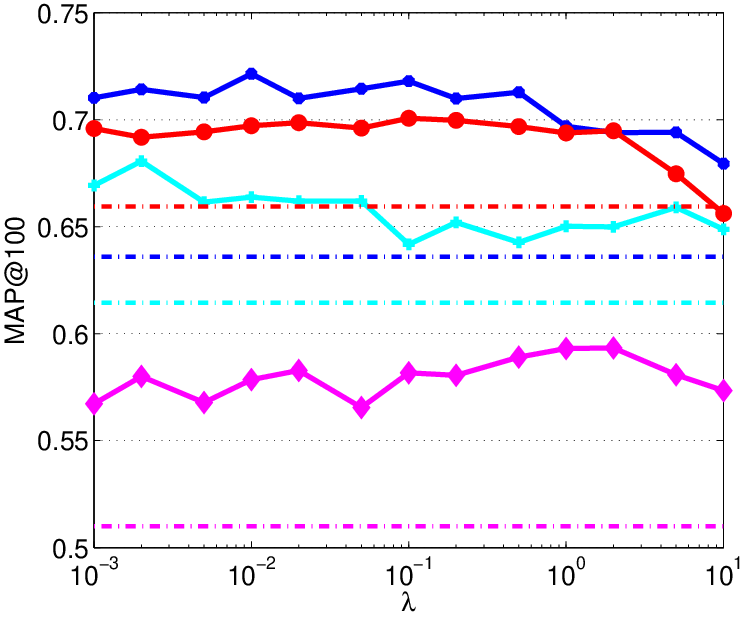
Parameter sensitive analysis. We also conduct the parameter sensitive analysis to show that our approach is robust to the change of parameters. The experiments are conducted on FLICKR$25K$ and NUS-WIDE using a validation set, to form which we randomly sample a subset of the training dataset. The size of the validation set is 1000 and 2000 respectively for FLICKR$25K$ and NUW-WIDE. To evaluate the sensitive of the parameter, we vary one parameter from 0.001 to 10 (1 for $\rho$) while keep others fixed.

The empirical results on the two search tasks (task1: image to text and task2: text to image) are presented in Figure 4. It can be seen from the figure that our approach can achieve superior performance under a wide range of the parameter values. We notice that when the parameter $\rho$ gets close to 1, the performance drops suddenly. The reason might be that with a larger sparsity degree value $\rho$, the learnt image representation in the common space would carry little information since the learnt $\mathbf{S}$ is a very sparse matrix.

7 Conclusion

In this paper, we present a quantization-based compact coding approach, collaborative quantization, for cross-modal similarity search. The superiority of the proposed approach stems from that it learns the quantizers for both modalities jointly by aligning the quantized approximations for each pair of image and text in the common space, which is simultaneously learnt with the quantization. Empirical results on three multi-modal datasets indicate that the proposed approach outperforms existing methods.

References

- [1] M. M. Bronstein, A. M. Bronstein, F. Michel, and N. Paragios. Data fusion through cross-modality metric learning using similarity-sensitive hashing. In CVPR, pages 3594–3601. IEEE Computer Society, 2010.
- [2] T.-S. Chua, J. Tang, R. Hong, H. Li, Z. Luo, and Y.-T. Zheng. Nus-wide: A real-world web image database from national university of singapore. In Proc. of ACM Conf. on Image and Video Retrieval (CIVR’09), Santorini, Greece., July 8-10, 2009.
- [3] M. Datar, N. Immorlica, P. Indyk, and V. S. Mirrokni. Locality-sensitive hashing scheme based on p-stable distributions. In Proceedings of the 20th ACM Symposium on Computational Geometry, Brooklyn, New York, USA, June 8-11, 2004, pages 253–262, 2004.
- [4] G. Ding, Y. Guo, and J. Zhou. Collective matrix factorization hashing for multimodal data. In 2014 IEEE Conference on Computer Vision and Pattern Recognition, CVPR 2014, Columbus, OH, USA, June 23-28, 2014, pages 2083–2090, 2014.
- [5] Y. Gong, S. Lazebnik, A. Gordo, and F. Perronnin. Iterative quantization: A procrustean approach to learning binary codes for large-scale image retrieval. IEEE Trans. Pattern Anal. Mach. Intell., 35(12):2916–2929, 2013.
- [6] H. Jégou, M. Douze, and C. Schmid. Product quantization for nearest neighbor search. IEEE Trans. Pattern Anal. Mach. Intell., 33(1):117–128, 2011.
- [7] S. Kim, Y. Kang, and S. Choi. Sequential spectral learning to hash with multiple representations. In Computer Vision - ECCV 2012 - 12th European Conference on Computer Vision, Florence, Italy, October 7-13, 2012, Proceedings, Part V, pages 538–551, 2012.
- [8] S. Kumar and R. Udupa. Learning hash functions for cross-view similarity search. In T. Walsh, editor, IJCAI, pages 1360–1365. IJCAI/AAAI, 2011.
- [9] Z. Lin, G. Ding, M. Hu, and J. Wang. Semantics-preserving hashing for cross-view retrieval. In IEEE Conference on Computer Vision and Pattern Recognition, CVPR 2015, Boston, MA, USA, June 7-12, 2015, pages 3864–3872, 2015.
- [10] M. Long, J. Wang, and P. S. Yu. Compositional correlation quantization for large-scale multimodal search. CoRR, abs/1504.04818, 2015.
- [11] J. Masci, M. M. Bronstein, A. M. Bronstein, and J. Schmidhuber. Multimodal similarity-preserving hashing. IEEE Trans. Pattern Anal. Mach. Intell., 36(4):824–830, 2014.
- [12] S. Moran and V. Lavrenko. Regularised cross-modal hashing. In Proceedings of the 38th International ACM SIGIR Conference on Research and Development in Information Retrieval, Santiago, Chile, August 9-13, 2015, pages 907–910, 2015.
- [13] M. Muja and D. G. Lowe. Fast approximate nearest neighbors with automatic algorithm configuration. In VISSAPP (1), pages 331–340, 2009.
- [14] M. Muja and D. G. Lowe. Scalable nearest neighbor algorithms for high dimensional data. IEEE Trans. Pattern Anal. Mach. Intell., 36(11):2227–2240, 2014.
- [15] M. Norouzi and D. J. Fleet. Minimal loss hashing for compact binary codes. In Proceedings of the 28th International Conference on Machine Learning, ICML 2011, Bellevue, Washington, USA, June 28 - July 2, 2011, pages 353–360, 2011.
- [16] M. Norouzi and D. J. Fleet. Cartesian k-means. In 2013 IEEE Conference on Computer Vision and Pattern Recognition, Portland, OR, USA, June 23-28, 2013, pages 3017–3024, 2013.
- [17] N. Rasiwasia, P. J. Moreno, and N. Vasconcelos. Bridging the gap: Query by semantic example. IEEE Transactions on Multimedia, 9(5):923–938, 2007.
- [18] N. Rasiwasia, J. C. Pereira, E. Coviello, G. Doyle, G. R. G. Lanckriet, R. Levy, and N. Vasconcelos. A new approach to cross-modal multimedia retrieval. In Proceedings of the 18th International Conference on Multimedia 2010, Firenze, Italy, October 25-29, 2010, pages 251–260, 2010.
- [19] J. Song, Y. Yang, Z. Huang, H. T. Shen, and J. Luo. Effective multiple feature hashing for large-scale near-duplicate video retrieval. IEEE Transactions on Multimedia, 15(8):1997–2008, 2013.
- [20] J. Song, Y. Yang, Y. Yang, Z. Huang, and H. T. Shen. Inter-media hashing for large-scale retrieval from heterogeneous data sources. In Proceedings of the ACM SIGMOD International Conference on Management of Data, SIGMOD 2013, New York, NY, USA, June 22-27, 2013, pages 785–796, 2013.
- [21] N. Srivastava and R. Salakhutdinov. Multimodal learning with deep boltzmann machines. Journal of Machine Learning Research, 15(1):2949–2980, 2014.
- [22] D. Wang, X. Gao, X. Wang, and L. He. Semantic topic multimodal hashing for cross-media retrieval. In Proceedings of the Twenty-Fourth International Joint Conference on Artificial Intelligence, IJCAI 2015, Buenos Aires, Argentina, July 25-31, 2015, pages 3890–3896, 2015.
- [23] J. Wang, S. Kumar, and S. Chang. Semi-supervised hashing for large-scale search. IEEE Trans. Pattern Anal. Mach. Intell., 34(12):2393–2406, 2012.
- [24] J. Wang and S. Li. Query-driven iterated neighborhood graph search for large scale indexing. In Proceedings of the 20th ACM Multimedia Conference, MM ’12, Nara, Japan, October 29 - November 02, 2012, pages 179–188, 2012.
- [25] J. Wang, H. T. Shen, J. Song, and J. Ji. Hashing for similarity search: A survey. CoRR, abs/1408.2927, 2014.
- [26] J. Wang, J. Wang, J. Song, X. Xu, H. T. Shen, and S. Li. Optimized cartesian k-means. IEEE Trans. Knowl. Data Eng., 27(1):180–192, 2015.
- [27] J. Wang, J. Wang, G. Zeng, R. Gan, S. Li, and B. Guo. Fast neighborhood graph search using cartesian concatenation. In ICCV, pages 2128–2135, 2013.
- [28] J. Wang, N. Wang, Y. Jia, J. Li, G. Zeng, H. Zha, and X.-S. Hua. Trinary-projection trees for approximate nearest neighbor search. IEEE Trans. Pattern Anal. Mach. Intell., 2013.
- [29] W. Wang, B. C. Ooi, X. Yang, D. Zhang, and Y. Zhuang. Effective multi-modal retrieval based on stacked auto-encoders. PVLDB, 7(8):649–660, 2014.
- [30] B. Wu, Q. Yang, W. Zheng, Y. Wang, and J. Wang. Quantized correlation hashing for fast cross-modal search. In Proceedings of the Twenty-Fourth International Joint Conference on Artificial Intelligence, IJCAI 2015, Buenos Aires, Argentina, July 25-31, 2015, pages 3946–3952, 2015.
- [31] F. Wu, Z. Yu, Y. Yang, S. Tang, Y. Zhang, and Y. Zhuang. Sparse multi-modal hashing. IEEE Transactions on Multimedia, 16(2):427–439, 2014.
- [32] D. Zhang and W. Li. Large-scale supervised multimodal hashing with semantic correlation maximization. In Proceedings of the Twenty-Eighth AAAI Conference on Artificial Intelligence, July 27 -31, 2014, Québec City, Québec, Canada., pages 2177–2183, 2014.
- [33] D. Zhang, F. Wang, and L. Si. Composite hashing with multiple information sources. In Proceeding of the 34th International ACM SIGIR Conference on Research and Development in Information Retrieval, SIGIR 2011, Beijing, China, July 25-29, 2011, pages 225–234, 2011.
- [34] T. Zhang, C. Du, and J. Wang. Composite quantization for approximate nearest neighbor search. In ICML (2), pages 838–846, 2014.
- [35] T. Zhang, G. Qi, J. Tang, and J. Wang. Sparse composite quantization. In IEEE Conference on Computer Vision and Pattern Recognition, CVPR 2015, Boston, MA, USA, June 7-12, 2015, pages 4548–4556, 2015.
- [36] Y. Zhen and D. Yeung. Co-regularized hashing for multimodal data. In Advances in Neural Information Processing Systems 25: 26th Annual Conference on Neural Information Processing Systems 2012. Proceedings of a meeting held December 3-6, 2012, Lake Tahoe, Nevada, United States., pages 1385–1393, 2012.
- [37] Y. Zhen and D.-Y. Yeung. A probabilistic model for multimodal hash function learning. In Q. Y. 0001, D. Agarwal, and J. Pei, editors, KDD, pages 940–948. ACM, 2012.
- [38] J. Zhou, G. Ding, and Y. Guo. Latent semantic sparse hashing for cross-modal similarity search. In The 37th International ACM SIGIR Conference on Research and Development in Information Retrieval, SIGIR ’14, Gold Coast , QLD, Australia - July 06 - 11, 2014, pages 415–424, 2014.
- [39] X. Zhu, Z. Huang, H. T. Shen, and X. Zhao. Linear cross-modal hashing for efficient multimedia search. In ACM Multimedia Conference, MM ’13, Barcelona, Spain, October 21-25, 2013, pages 143–152, 2013.