Structure learning via unstructured kernel-based M-regression

Abstract

In statistical learning, identifying underlying structures of true target functions based on observed data plays a crucial role to facilitate subsequent modeling and analysis. Unlike most of those existing methods that focus on some specific settings under certain model assumptions, this paper proposes a general and novel framework for recovering true structures of target functions by using unstructured M-regression in a reproducing kernel Hilbert space (RKHS). The proposed framework is inspired by the fact that gradient functions can be employed as a valid tool to learn underlying structures, including sparse learning, interaction selection and model identification, and it is easy to implement by taking advantage of the nice properties of the RKHS. More importantly, it admits a wide range of loss functions, and thus includes many commonly used methods, such as mean regression, quantile regression, likelihood-based classification, and margin-based classification, which is also computationally efficient by solving convex optimization tasks. The asymptotic results of the proposed framework are established within a rich family of loss functions without any explicit model specifications. The superior performance of the proposed framework is also demonstrated by a variety of simulated examples and a real case study.

Key Words and Phrases: Convex optimization, gradient learning, high-dimension, reproducing kernel Hilbert space, screening, structure learning

1 Introduction

In statistical learning, true target functions are often assumed to have some specific structures to facilitate the following statistical modeling and analysis. Thus, tremendous interests have been paid to recover underlying structures from observed data, including learning sparse structures (Li et al. 2012; He et al. 2013; Wang and Leng 2016; Dasgupta et al. 2019; Han 2019; Pan et al. 2019; Tang et al. 2021), interaction effects (Lin and Zhang 2006; Radchenko and James 2010; Hao and Zhang 2014; Kong et al. 2017; Hao et al. 2018) or identifying linear and nonlinear effects (Zhang et al. 2011; Lian et al. 2015; He and Wang 2020). However, most existing methods are designed for learning some specific structures, and their successes either reply on restrictive model assumptions or require intensive computational efforts. For example, various attempts have been made to learn the sparsity of the conditional mean function by regularization (Fan and Lv 2010), screening (Fan and Lv 2008; Wang and Leng 2016), or checking variable robustness against added noises (Barber and Cand ¨ e s 2015). The counterparts of these methods have also been proposed in the context of quantile regression (Wu and Liu 2009; Ma et al. 2017), margin-based classification (Steinwart and Christmann 2008b; Zhang et al. 2016b), generalized linear models (Li and Liu 2019) and so on. Furthermore, the additive model assumption is often imposed to relax the linear assumption in pursuing sparsity (Huang et al. 2010; Fan et al. 2011; Lv et al. 2018). However, all these methods are only designed for some specific learning tasks and lack of universality. Most recently, tremendous attentions have been paid to tackle the universality issue. Loh 2017 focuses on the theoretical aspect of regularized linear M-estimators within a family of robust loss functions. Dasgupta et al. 2019 propose a recursive feature elimination method via repeatedly fitting a kernel ridge regression for a general loss function, but the computational efficiency becomes its main obstacle. Han 2019 proposes a novel nonparametric screening method under a strictly convex loss function family, but it requires the loss function to be differentiable almost everywhere, which excludes some popular loss functions, such as the hinge loss. Other popularly assumed structures of the true target function include the interaction structure (Lin and Zhang 2006; Radchenko and James 2010; Hao et al. 2018; Hao and Zhang 2014; Kong et al. 2017; Dong and Wu 2021) and the model identification by identifying linear or nonlinear effects (Zhang et al. 2011; Lian et al. 2015; He and Wang 2020), and these methods are developed in a similar way to the sparse learning. However, these methods are also designed for some specific scenarios, and the lack of theoretical consistency or computational efficiency becomes their main obstacle.

Recently, many kernel-based sparse learning methods have been motivated by the fact that gradient functions provide an appropriate tool to identify informative variables in a model-free fashion, and thus various strategies have been adopted to learn the gradient functions under some specific scenarios. For example, Rosasco et al. 2013 add an empirical functional penalty on the gradients in a standard kernel ridge regression, and He et al. 2020 further extend it to learn the sparse structure in support vector machines. Yang et al. 2016 employ a pair-wise learning task to estimate gradient functions and use a functional group lasso penalty to induce sparsity, and He and Wang 2020 extend it to learn interaction structures. Most recently, He et al. 2021 propose an efficient two-step sparse learning method in the least square regression. Clearly, all these sparse learning methods are methodologically flexible in the sense that they rely on no model specifications, and thus are applicable to datasets with complicated dependence patterns. However, these methods are developed under specific scenarios in regression or classification, and their high computational costs or lack of consistency and universality are still unsolved issues.

This paper proposes a novel structure learning framework via the regularized M-regression for a general family of loss functions in a flexible RKHS. The proposed framework is inspired by the fact that gradient functions characterize structures of their corresponding true target functions without explicit model assumptions, and the derivative reproducing properties of the RKHS (Zhou 2007) facilitate the computation of gradient functions. The proposed framework is methodologically simple, and computationally easy to implement, which can also be scaled up by a parallelization procedure. Specifically, it consists of estimation of the regularized M-regression in a RKHS, and computation of the gradient functions by a matrix multiplication. It is computationally efficient by only fitting a standard kernel ridge regression via solving a convex optimization problem, and thus scalable to analyze large-scale datasets. More importantly, the asymptotic properties of the proposal in sparse learning, interactions selection and model identification are established based on a general family of loss functions without imposing any explicit model assumptions.

The major contributions of the proposed framework are four-fold.

1. It works for a general loss function family including most commonly used ones in literature, such as the squared loss, check loss, hinge loss, Huber loss, logistic loss, $\epsilon$-insensitive loss, exponential loss and so on.

2. It establishes a unified framework for learning underlying structures of true target functions and admits general dependence structures. The proposed framework employs gradient functions to recover the structures in a model-free fashion and can be regarded as a joint screening method and thus is able to identify all the informative variables acting on the response with a general dependence structure, including those marginally noninformative but jointly informative ones.

3. It is methodologically simple and computationally easy to implement. Specifically, it avoids directly estimating gradient functions, but solving a kernel-based convex optimization problem. Then, the estimated gradient functions can be efficiently obtained by using the derivative reproducing properties of the RKHS, which significantly reduces the computational costs. For instance, in Examples 1 and 2 of our simulation study, the proposed framework is efficiently implemented to sparse learning with dimensionality up to $10^{5}$.

4. It provides theoretical guarantees for structure learning under mild conditions. With the help of empirical process and functional operators in learning theory, the estimation consistency of gradient functions is established for a general loss function family. More importantly, as a direct consequence, the asymptotic consistencies of sparse learning, interaction selection and model identification are established without imposing any explicit model specifications.

The rest of this paper is organized as follows. Section 2 introduces the rich family of loss functions and illustrates the connections between gradient functions and the corresponding functional structures. Section 3 introduces the motivations and the proposed structure learning framework. All the computational details are provided in Section 4. In Section 5, the asymptotic theoretical results of the proposed method are given. The simulated examples and a real case study are provided in Section 6. A brief discussion is provided in Section 7, and extra numerical results and all the technical proofs of Theorems 1–5 are deferred to the Supplementary Material. An R package implementing the proposed method is available at https://github.com/geyh96/GSLM/.

2 Preambles and Methodology

2.1 A rich family of loss functions

Suppose a random pair ${\cal Z}=(\mathop{\bf x},y)$ is drawn from some unknown joint distribution $\rho_{\mathop{\bf x},y}$, with ${\mathop{\bf x}}=(x_{1},...,x_{p})^{T}\in{\cal X}$ supported on a compact subset of ${\cal R}^{p}$ and $y\in{\cal Y}\subset{\cal R}$. In statistical learning, the true target function $f^{*}$ is often defined as the minimizer of the following expected error

$${f^{*}=\mathop{\rm argmin}{\cal E}^{L}(f)=\mathop{\rm argmin}EL(y,f(\mathop{\bf x})),}$$ (1)

where ${L}(\cdot,\cdot):{\cal Y}\times{\cal R}\rightarrow{\cal R}^{+}$ is the loss function of our interests. We first impose the following conditions on the loss $L$.
Assumption 1: The loss function ${L}$ satisfies the following two conditions.

• There exist some positive constants $c_{1}$ and $q\geq 1$ such that ${L}(y,\omega)\leq c_{1}(|y|^{q}+|\omega|^{q})$, for any $y\in{\cal Y}$ and $\omega\in{\cal R}$.

• ${L}(y,\cdot)$ is convex, and locally Lipschitz continuous; that is, for any ${V}\geq 0$, there exists a constant $c_{2}>0$ such that $\left|{L}(y,\omega)-{L}(y,\omega{{}^{\prime}})\right|\leq c_{2}|\omega-\omega{{}^{\prime}}|$, for any $\omega,{\omega}{{}^{\prime}}\in[-V,V]$ and $y\in{\cal Y}$.

Note that the above conditions are mild and commonly used in literature to characterize loss functions (Hang and Steinwart 2018; Dasgupta et al. 2019). The loss space satisfying these two conditions include many popular losses:

(i) Squared loss: ${L}(y,f(\mathop{\bf x}))=(y-f(\mathop{\bf x}))^{2}$ with $c_{2}=2(M_{y}+V)$ and $q=2$, for any $|y|\leq M_{y}$ with a positive constant $M_{y}$;

(ii) Check loss: ${L}_{\tau}(y,f(\mathop{\bf x}))=(y-f(\mathop{\bf x}))(\tau-I_{\{y<f(\mathop{\bf x})\}})$ with $c_{2}=1$ and $q=1$;

(iii) Huber loss: ${L}(y,f(\mathop{\bf x}))=(y-f(\mathop{\bf x}))^{2}$, if $|y-f(\mathop{\bf x})|\leq{\delta}$; $\delta|y-f(\mathop{\bf x})|-\frac{1}{2}\delta^{2}$, otherwise, with $c_{2}=\delta$ and $q=1$;

(iv) $\epsilon$-insensitive loss: ${L}(y,f(\mathop{\bf x}))=\max\{0,|y-f(\mathop{\bf x})|-\epsilon\}$ with $c_{2}=1$ and $q=1$;

(v) Logistic loss: ${L}(y,f(\mathop{\bf x}))=(\ln 2)^{-1}\log\big(1+\exp{(-yf(\mathop{\bf x})})\big)$ with $c_{2}=(\ln 2)^{-1}e^{V}/(1+e^{V})$ and $q=1$;

(vi) Hinge loss: ${L}(y,f(\mathop{\bf x}))=(1-yf(\mathop{\bf x}))_{+}$ with $c_{2}=1$ and $q=1$;

(vii) Exponential loss: ${L}(y,f(\mathop{\bf x}))=\exp{(-yf(\mathop{\bf x}))}$ with $c_{2}=e^{V}$ and $q=1$.

The explicit form of $f^{*}$ varies from one loss function to another. For example, when the squared loss is used, $f^{*}(\mathop{\bf x})=E(y|\mathop{\bf x})$; when the check loss is used, $f^{*}(\mathop{\bf x})=Q_{\tau}(y|\mathop{\bf x})$ with $Q_{\tau}(y|\mathop{\bf x})=\inf\{y:P(Y\leq y|\mathop{\bf x})\geq\tau\}$; and when the hinge loss is used, $f^{*}(\mathop{\bf x})=\mathop{\rm sign}(P(y=1|\mathop{\bf x})-1/2)$, where $\mathop{\rm sign}(\cdot)$ is the sign function. In this paper, we assume that $f^{*}\in{\cal H}_{K}$, where ${\cal H}_{K}$ denotes the RKHS induced by a pre-specified kernel function $K(\cdot,\cdot)$. This requirement is commonly used in statistical learning literature (Rosasco et al. 2013; Yang et al. 2016; Dasgupta et al. 2019), and it is well-known that the RKHS induced by some universal kernels, such as the Gaussian kernel, is a fairly large functional space in that any continuous function can be arbitrarily well approximated by an intermediate function in its induced RKHS under the infinity norm (Steinwart 2005).

2.2 Structure learning via gradient functions

In statistical analysis, the true target function $f^{*}$ is often assumed to have a specific structure and tremendous interests have been paid to recover the structure of $f^{*}$ from the observed data, including learning the sparse/interaction structure of $f^{*}$ or identifying the linear and nonlinear effects in $f^{*}$. Unlike most of existing methods that only work under specific settings and model assumptions, we observe that the gradient functions can be employed as an efficient and flexible tool to meet these statistical interests. Precisely, for the true target function $f^{*}$ defined in (1) with a loss function satisfying Assumption 1, we focus on the first- and second- order gradient functions of $f^{*}$ that

$$g^{*}_{l}(\mathop{\bf x})=\frac{\partial f^{*}(\mathop{\bf x})}{\partial x^{l}}\ \mbox{and}\ \ g^{*}_{lk}(\mathop{\bf x})=\frac{\partial^{2}f^{*}(\mathop{\bf x})}{\partial x^{l}\partial x^{k}},$$ (2)

for $l,k=1,...,p$. In the following, we illustrate how to use $g^{*}_{l}(\mathop{\bf x})$ and $g^{*}_{lk}(\mathop{\bf x})$ to conduct sparse learning, interaction selection and model identification in the sequential.

Example 2.1.

In sparse learning, it is generally believed that only a few variables have effect on $f^{*}$, while others are noises (Li et al. 2012; He et al. 2013). By using the first-order gradient function in (2), we observe that a variable $x^{l}$ does not contribute to the true target function $f^{*}$ if and only if

$$\|g^{*}_{l}\|^{2}_{{\cal L}^{2}({\cal X},\rho_{\mathop{\bf x}})}=\int_{\cal X}(g_{l}^{*}(\mathop{\bf x}))^{2}d\rho_{\mathop{\bf x}}=0,$$ (3)

where $\|\cdot\|^{2}_{{\cal L}^{2}({\cal X},\rho_{\mathop{\bf x}})}$ denotes the ${\cal L}^{2}({\cal X},\rho_{\mathop{\bf x}})$-norm and $\rho_{\mathop{\bf x}}$ denotes the marginal distribution of the covariate $\mathop{\bf x}$. Thus, evaluating the importance of a variable turns to measure the importance of the corresponding gradient function, and thus $\|g^{*}_{l}\|^{2}_{{\cal L}^{2}({\cal X},\rho_{\mathop{\bf x}})}$ can be adopted as a valid measure to distinguish the informative and noninformative variables in $f^{*}$. Then the true active set can be defined as ${\cal A}^{*}=\{l:\left\|g^{*}_{l}\right\|^{2}_{{\cal L}^{2}({\cal X},\rho_{\mathop{\bf x}})}>0\}$,

Example 2.2.

For interaction selection, many attempts have been made to identify the true interaction effects in underlying models (Lin and Zhang 2006; Radchenko and James 2010; Hao and Zhang 2014; Kong et al. 2017; Hao et al. 2018; Dong and Wu 2021). We observe that the true interaction effects on $f^{*}$ can be evaluated by the second-order gradient functions. Specifically, given the true active set ${\cal A}^{*}$, if a variable $x^{l}$ has no interaction effect on $f^{*}$, the corresponding second-order gradient functions among all the other variables should be zero almost surely in the sense that

$$\|g^{*}_{lk}\|^{2}_{{\cal L}^{2}({\cal X},\rho_{\mathop{\bf x}})}=\int_{\cal X}(g^{*}_{lk}(\mathop{\bf x}))^{2}d\rho_{\mathop{\bf x}}=0,$$ (4)

for any $k\in{\cal A}^{*}$. Thus, the active set containing all the variables that contribute to the two-way interaction effects in $f^{*}$ can be defined as

$${\cal A}^{*}_{2}=\big\{l\in{\cal A}^{*}:\|g^{*}_{lk}\|^{2}_{{\cal L}^{2}({\cal X},\rho_{\mathop{\bf x}})}>0,~\mbox{for some}\ k\in{\cal A}^{*}\big\},$$

Moreover, we further denote the set containing the variables that only contribute to the main effects of $f^{*}$as ${\cal A}_{1}^{*}={\cal A}^{*}\setminus{\cal A}^{*}_{2}$. It is interesting to point out that the definitions of ${\cal A}^{*}_{1}$ and ${\cal A}^{*}_{2}$ are general and reduce to those in Kong et al. 2017 when the true structure of $f^{*}$ is a quadratic function.

Example 2.3.

Identifying the linear and nonlinear effects in $f^{*}$ has also attracted many attentions in the literature of partially linear models (PLMs) (Zhang et al. 2011; Lian et al. 2015; He and Wang 2020). Generally, a PLM considers

$$f^{*}(\mathop{\bf x})={\mathop{\bf x}}^{T}_{\cal L^{*}}{\mbox{\boldmath$\beta$}}^{*}+h^{*}({\mathop{\bf x}}_{\cal N^{*}}),$$

where $\mathop{\bf x}=({\mathop{\bf x}}_{\cal L^{*}}^{T},{\mathop{\bf x}}_{\cal N^{*}}^{T})^{T}\in{\cal R}^{p}$, ${\cal L^{*}}^{*}$ and ${\cal N}^{*}$ denote the sets of linear and nonlinear effects, ${\mathop{\bf x}}^{T}_{\cal L}{\mbox{\boldmath$\beta$}}^{*}$ is the linear part and $h^{*}({\mathop{\bf x}}_{\cal N}^{*})$ is the nonlinear part. One of the primal interests is to correctly identify the linear and nonlinear effects in a PLM. We notice that the true linear and nonlinear effects can be distinguished by evaluating the corresponding second-order gradient functions. Specifically, given the true active set ${\cal A}^{*}$, we observe that if a variable $x_{l}$ has a linear effect on $f^{*}$, the corresponding second-order gradient functions among all the other variables should be zero almost surely that $\|g^{*}_{lk}\|^{2}_{{\cal L}^{2}({\cal X},\rho_{\mathop{\bf x}})}=0$ for any $k\in{\cal A}^{*}$. Thus, the sets of true linear effects and true nonlinear effects can be defined as ${\cal L}^{*}=\{l:\|g^{*}_{lk}\|^{2}_{{\cal L}^{2}({\cal X},\rho_{\mathop{\bf x}})}=0,~\text{for any}~k\in{\cal A}^{*}\}$ and ${\cal N}^{*}={\cal A}^{*}\backslash{\cal L}^{*}$.

As demonstrated in the above examples, the gradient functions can be employed as an efficient and flexible tool to learn the interested structure of $f^{*}$ and more importantly, it provides appropriate definitions of the interested structure of $f^{*}$ in a “model-free” sense, which avoids the risk of potential model misspecifications. Thus, it suffices to learn the corresponding gradient functions consistently and efficiently for identifying the underlying structure of $f^{*}$.

3 The Proposed Framework

Most existing learning gradient methods formulate the task into a regularized framework (Rosasco et al. 2013; Yang et al. 2016; He and Wang 2020; He et al. 2020) with some carefully designed functional penalties on the gradient functions. However, these methods usually suffer computational burdens due to the employed local pair-wise learning tasks or the added complicated empirical functional penalties. On the contrary, the proposed framework provides an efficient alternative to learning the structure of $f^{*}$. It is motivated by the key observations that the derivative reproducing properties in RKHS (Zhou 2007) assure that if $K(\cdot,\cdot)\in{C}^{2}({\cal X},{\cal X})$, then for any $f\in{\cal H}_{K}$, there holds

$$g_{l}(\mathop{\bf x})=\frac{\partial f(\mathop{\bf x})}{\partial x^{l}}=\langle f,{\partial_{l}{K}_{\mathop{\bf x}}}\rangle_{K},$$ (5)

where ${C}^{2}$ denotes the class of functions whose second derivative is continuous and ${\partial_{l}{K}_{\mathop{\bf x}}(\cdot)}=\frac{\partial K(\mathop{\bf x},\cdot)}{\partial x^{l}}\in{\cal H}_{K}$. Moreover, if $K(\cdot,\cdot)\in{C}^{4}({\cal X},{\cal X})$, there also holds that

$$g_{lk}(\mathop{\bf x})=\frac{\partial f(\mathop{\bf x})}{\partial x^{l}\partial x^{k}}=\langle f,{\partial_{lk}{K}_{\mathop{\bf x}}}\rangle_{K},$$ (6)

where $\partial_{lk}K_{\mathop{\bf x}}=\frac{\partial K(\mathop{\bf x},\cdot)}{\partial x^{l}\partial x^{k}}\in{\cal H}_{K}$. Note that the facts (5) and (6) assure that to estimate the interested gradient functions within the induced RKHS, it suffices to estimate the target function $f$ itself, and then the gradient functions can be directly obtained. In the rest of this paper, we focus on the applications of the first- and second-order gradient functions to learn the structure of $f^{*}$ and thus assume that $K(\cdot,\cdot)\in{C}^{4}({\cal X},{\cal X})$, which is naturally satisfied by many kernels, including the Gaussian kernel. Note that it is trivial to extend the proposed framework to estimate arbitrary higher-order gradient functions, which may be useful in some real applications (Ritchie et al. 2001).

Motivated by these key facts, we propose an efficient framework to learn the underlying structure of the true target function $f^{*}$, which involves a regularized M-estimation in the induced RKHS and the fast computation of corresponding gradient functions. Suppose that the random sample ${\cal Z}^{n}=\{({\mathop{\bf x}}_{i},y_{i})\}_{i=1}^{n}$ are independent copies of the random pair $(\mathop{\bf x},y)$. Firstly, we consider the regularized M-estimation in a RKHS to estimate $f^{*}$ by solving the following optimization problem that

$$\widehat{f}=\mathop{\rm argmin}_{f\in{\cal H}_{K}}\frac{1}{n}\sum_{i=1}^{n}{L}\left(y_{i},f({\mathop{\bf x}}_{i})\right)+\lambda\|f\|_{K}^{2},$$ (7)

where the first term is denoted as ${\cal E}^{L}_{{\cal Z}^{n}}(f)$ and $\|\cdot\|_{K}$ denotes the induced RKHS-norm. By the representer theorem (Wahba MIT Press, 1998), the solution of (7) must have a finite form that

$$\widehat{f}(\mathop{\bf x})=\sum_{i=1}^{n}\widehat{\alpha}_{i}K({\mathop{\bf x}}_{i},\mathop{\bf x})=\widehat{\mbox{\boldmath$\alpha$}}^{T}{\mathop{\bf K}}_{n}(\mathop{\bf x}),$$ (8)

where $\widehat{\mbox{\boldmath$\alpha$}}=(\widehat{\alpha}_{1},...,\widehat{\alpha}_{n})^{T}$ denotes the representer coefficients and ${\mathop{\bf K}}_{n}(\mathop{\bf x})=(K({\mathop{\bf x}}_{1},\mathop{\bf x}),...,K({\mathop{\bf x}}_{n},\mathop{\bf x}))^{T}$ is the $n$-deimensional kernel vector.

Then, we apply the derivative reproducing properties (5) and (6) to facilitate the computation of gradient functions of our interests. Specifically, once $\widehat{\mbox{\boldmath$\alpha$}}$ is obtained, we can efficiently compute the estimated first- and second-order gradient functions that

$$\widehat{g}_{l}(\mathop{\bf x})=\frac{\partial\widehat{f}(\mathop{\bf x})}{\partial x^{l}}=\widehat{\mbox{\boldmath$\alpha$}}^{T}{\partial_{l}{\mathop{\bf K}}_{n}({\mathop{\bf x}}})\ ~\mbox{and}~\ \widehat{g}_{lk}(\mathop{\bf x})=\frac{\partial^{2}\widehat{f}(\mathop{\bf x})}{\partial x^{l}\partial x^{k}}=\widehat{\mbox{\boldmath$\alpha$}}^{T}{\partial_{lk}{\mathop{\bf K}}_{n}({\mathop{\bf x}})},$$

where ${\partial_{l}{\mathop{\bf K}}_{n}({\mathop{\bf x}}})=\frac{\partial{\mathop{\bf K}}_{n}({\mathop{\bf x}})}{\partial x^{l}}\in{\cal R}^{n}$ and $\partial_{lk}\mathop{\bf K}_{n}(\mathop{\bf x})=\frac{\partial^{2}{\mathop{\bf K}}_{n}({\mathop{\bf x}})}{\partial x^{l}\partial x^{k}}\in{\cal R}^{n}$. Note that once the kernel function $K(\cdot,\cdot)$ is pre-specified, the corresponding gradients $\partial_{l}\mathop{\bf K}_{n}(\mathop{\bf x})$ and $\partial_{lk}\mathop{\bf K}_{n}(\mathop{\bf x})$ are also analytically determined.

Now we illustrate how to apply the estimated gradient functions to recover the underlying structure of the true target function $f^{*}$ in Examples 2.1–2.3. Precisely, for sparse learning, we adopt the empirical norm of $\widehat{g}_{l}$ as a practical measure by computing $\|\widehat{g}_{l}\|^{2}_{n}=\frac{1}{n}\sum_{i=1}^{n}\big(\widehat{g}_{l}(\mathop{\bf x}_{i})\big)^{2}$, and thus the estimated active set is defined as $\widehat{\cal A}=\left\{l:\left\|\widehat{g}_{l}\right\|^{2}_{n}>v_{n}\right\}$, where $v_{n}$ denotes some pre-specified thresholding value; for interaction selection, we adopt the empirical norm of the estimated second-order gradient function by computing $\|\widehat{g}_{lk}\|^{2}_{n}=\frac{1}{n}\sum_{i=1}^{n}\big(\widehat{g}_{lk}({\mathop{\bf x}}_{i})\big)^{2}$, and thus the sets of active interaction and main effects in $f^{*}$ can be estimated as

$$\widehat{\cal A}_{2}=\big\{l\in\widehat{\cal A}:\|\widehat{g}_{lk}\|^{2}_{n}>v_{n}^{int},~\mbox{for some}\ k\in\widehat{\cal A}\big\}\ \mbox{and}\ \widehat{\cal A}_{1}=\widehat{\cal A}\setminus\widehat{\cal A}_{2},$$

respectively, where $v_{n}^{int}$ denotes some pre-specified thresholding value. Moreover, we can also apply the estimated second-order gradient functions to conduct model identification, and thus the estimated nonlinear and linear effect sets ${\cal N}^{*}$ and ${\cal L}^{*}$ are identified as $\widehat{\cal N}=\big\{l\in\widehat{\cal A}:\|\widehat{g}_{lk}\|^{2}_{n}>v_{n}^{iden},~\mbox{for some}\ k\in\widehat{\cal A}\big\}\ \mbox{and}\ \widehat{\cal L}=\widehat{\cal A}\setminus\widehat{\cal N},$ respectively, where $v_{n}^{iden}$ is the pre-defined thresholding value. Note that the structure learning performance of the proposed method highly relies on the choice of pre-specified thresholding values, which can be appropriately determined through a stability-based selection criterion (Sun et al. 2013) and more details are provided in Section 4.2.

4 Computational Issues

In this section, we provide all the computational details as well as the tuning procedures of the proposed framework.

4.1 Computing algorithms

Note that the proposed framework is computationally efficient in that we only need to solve a convex optimization problem (7), and then the estimated gradient functions can be directly obtained with the derivative reproducing property of the RHKS. More importantly, by the representer theorem, the original optimization task over an infinite function space ${\cal H}_{K}$ is converted to an optimization task over a finite $n$-dimensional vector space of $\mbox{\boldmath$\alpha$}\in{\cal R}^{n}$. Specifically, by plugging (8) into (7), solving the optimization task (7) is equivalent to solving

$$\widehat{\mbox{\boldmath$\alpha$}}=\mathop{\rm argmin}_{\mbox{\boldmath$\alpha$}\in{\cal R}^{n}}\frac{1}{n}\sum_{i=1}^{n}{L}\left(y_{i},{\mbox{\boldmath$\alpha$}}^{T}{\mathop{\bf K}}_{n}(\mathop{\bf x})\right)+\lambda\mbox{\boldmath$\alpha$}^{T}\mathop{\bf K}\mbox{\boldmath$\alpha$},$$ (9)

where $\mathop{\bf K}=\{K(\mathop{\bf x}_{i},\mathop{\bf x}_{j})\}_{i,j=1}^{n}\in{\cal R}^{n\times n}$. Note that the employed computing algorithm for (9) varies from one loss function to another. For example, for the squared loss function, the solution to (9) has an explicit form that $\widehat{\mbox{\boldmath$\alpha$}}=(\mathop{\bf K}^{2}+n\lambda\mathop{\bf I}_{n})^{-1}\mathop{\bf K}\mathop{\bf y}$; for the check and hinge loss functions, the dual optimization can be considered (Takeuchi et al. 2006; Boyd and Vandenberghe 2004), which converts (9) to a quadratic programming problem with certain linear constraints; for the logistic loss, the kernel-based weighted least-square iterations (Zhu and Hastie 2005) can be employed. Note that the optimization task (9) can be efficiently implemented by using some disciplined convex optimization algorithms, and the R package CVXR (Fu et al. 2020) is used to carry out the optimization of the proposed framework in all the numerical examples of this paper.

4.2 Tuning procedure

It is interesting to notice that the proposed structure learning framework involves two tuning parameters that the parameter $\lambda$ in (9) and the pre-defined thresholding value used to define active sets of variables. Due to our limited numerical experience, the performance of the proposed framework is satisfactory when $\lambda$ is sufficiently small in various scenarios. Similar observation has also been made in Wang and Leng 2016. Thus, we use $\lambda=10^{-5}$ in Section 6, which yields satisfying performance.

Moreover, we employ the stability-based criterion (Sun et al. 2013) to select the optimal value of thresholding parameter. Its key idea is to measure the stability of sparse learning by randomly splitting the training sample into two parts and comparing the disagreement between these two estimated active sets. Specifically, given a thresholding value $v_{n}$, we randomly split the training sample ${\cal Z}^{n}$ into two parts ${\cal Z}^{n}_{1}$ and ${\cal Z}^{n}_{2}$. Then the proposed method is applied to ${\cal Z}^{n}_{1}$ and ${\cal Z}^{n}_{2}$ and obtain two estimated active sets $\widehat{\cal A}_{1,v_{n}}$ and $\widehat{\cal A}_{2,v_{n}}$, respectively. The disagreement between $\widehat{\cal A}_{1,v_{n}}$ and $\widehat{\cal A}_{2,v_{n}}$ is measured by Cohen’s kappa coefficient and the procedure is repeated for multiple times, and then the optimal thresholding value can be determined correspondingly. We refer to Sun et al. 2013 for more details.

5 Statistical Properties

In this section, we provide the theoretical guarantees of the proposed structure learning framework. Precisely, we establish the estimation consistency of gradient functions and provide the asymptotic consistencies of sparse learning, interaction selection and model identification under mild conditions, respectively.

We start with a brief introduction about some basic knowledge in learning theory. Specifically, we have $K(\mathop{\bf x},\cdot)\in{\cal H}_{K}$ for any ${\mathop{\bf x}}\in{\cal X}$, and $\langle f,{K}_{\mathop{\bf x}}\rangle_{K}=f(\mathop{\bf x})$ for any $f\in{\cal H}_{K}$. By Mercer’s theorem (Steinwart and Christmann 2008a), under some regularity conditions, the eigen-expansion of the kernel function is given by

$$K(\mathop{\bf x},\mathop{\bf x})=\sum_{k=1}^{\infty}\mu_{k}\phi_{k}(\mathop{\bf x})\phi_{k}(\mathop{\bf x}),$$ (10)

where $\mu_{1}\geq\mu_{2}\geq...\geq 0$ are non-negative eigenvalues, and $\{\phi_{k}\}_{k=1}^{\infty}$ are the associated eigenfunctions, taken to be orthonormal in ${\cal L}^{2}({\cal X},\rho_{\mathop{\bf x}})=\big\{f:\|f\|_{2}^{2}<\infty\big\}$. The RKHS-norm of any $f\in{\cal H}_{K}$ then can be written as

$$\|f\|^{2}_{K}=\sum_{k\geq 1}\frac{1}{\mu_{k}}\langle f,\phi_{k}\rangle^{2}_{{\cal L}^{2}({\cal X},\rho_{\mathop{\bf x}})},$$

which implies that the decay rate of $\mu_{k}$ fully characterizes the complexity of the RKHS induced by $K$, and has a close relationship with various entropy numbers (Steinwart and Christmann 2008a). Therefore, for any $f\in{\cal H}_{K}$, we have $f(\mathop{\bf x})=\sum_{k=1}^{\infty}a_{k}\phi_{k}(\mathop{\bf x}),$ where $a_{k}=\langle f,\phi_{k}\rangle_{{\cal L}^{2}({\cal X},\rho_{\mathop{\bf x}})}={\int}_{\cal X}f(\mathop{\bf x})\phi_{k}(\mathop{\bf x})d\rho_{\mathop{\bf x}}$ are Fourier coefficients. Note that these results require that ${\cal H}_{K}\subset{\cal L}^{2}({\cal X},\rho_{\mathop{\bf x}})$, which is automatically satisfied if $\sup_{\mathop{\bf x}\in{\cal X}}K(\mathop{\bf x},\mathop{\bf x})$ is bounded. Moreover, the solution of (1) may not be unique, and thus we further define $f^{*}=\mathop{\rm argmin}_{f\in{\cal B}}\|f\|_{K}^{2}$ with ${\cal B}=\{f:f=\mathop{\rm argmin}_{h\in{\cal H}_{K}}{\cal E}^{L}(h)\}$ to ensure the uniqueness of $f^{*}$ in the sequel. Furthermore, we denote $\widetilde{f}=\mathop{\rm argmin}_{f\in{\cal H}_{K}}{\cal E}^{L}(f)+\lambda\|f\|_{K}^{2}$. We now rewrite $\lambda$ as $\lambda_{n}$ in the rest of this paper, to emphasize its dependency on $n$.

5.1 Estimation consistency of gradient functions

The following technical assumptions are made to establish the estimation consistencies of gradient functions, which is crucial to ensure the asymptotic consistency of the proposed structure learning framework. We further introduce following assumptions.

Assumption 2: There exist some positive constants $\kappa_{1}$ and $\kappa_{2}$ such that $\sup_{\mathop{\bf x}\in{\cal X}}\|K_{\mathop{\bf x}}\|_{K}\leq\kappa_{1}$ and $\sup_{\mathop{\bf x}\in{\cal X}}\|\partial_{l}K_{\mathop{\bf x}}\|_{K}\leq\kappa_{2}$ for any $l=1,...,p$.

Assumption 3: There exist some positive constants $c_{3}$ and $\theta$ such that the approximation error $\|\widetilde{f}-f^{*}\|_{K}=c_{3}\lambda_{n}^{\theta}$.

Assumption 2 imposes the boundedness condition on the kernel function as well as the corresponding gradient functions. This assumption is commonly used in machine learning literature (Rosasco et al. 2013; Yang et al. 2016) and satisfied by many kernels with the compact support condition, including the Gaussian kernel, Sobolev kernel, scaled linear kernel, scaled quadratic kernel and so on. Note that the requirement of compact support is usually assumed in machine learning literature for mathematical simplicity, and many efforts have been made to extend it to the non-compact setting (Simon-Gabriel and Schölkopf 2018). Assumption 3 quantifies the approximation error as a function of the tuning parameter $\lambda_{n}$, which is sensible as $\lim_{\lambda_{n}\rightarrow 0}\|\widetilde{f}-f^{*}\|^{2}_{K}=0$ in general. Similar assumptions are also used in literature to control the approximation error rate (Mendelson and Neeman 2010; Rosasco et al. 2013; Zhang et al. 2016a; Dasgupta et al. 2019). Particularly, Mendelson and Neeman 2010 prove that the approximation error under the squared loss function can be explicitly quantified as $O(\lambda_{n}^{r-1/2})$ with $r\in(1/2,1]$. Further investigations about the approximation error rate are provided in Eberts and Steinwart 2013 by imposing some additional technical assumptions.

Theorem 1.

Suppose that Assumptions 1–3 are satisfied. Let $\lambda_{n}=n^{-1/(4q)}$, then for any $\delta_{n}\geq 2(\log n)^{-1/q}E|y|$, there exists some positive constant $c_{4}$ such that with probability at least $1-\delta_{n}$, such that the following inequality holds

$$\max_{l=1,...p}\Big|\|\widehat{g}_{l}\|^{2}_{n}-\|g^{*}_{l}\|^{2}_{{\cal L}^{2}({\cal X},\rho_{\mathop{\bf x}})}\Big|\leq{c_{4}}\left(\log\frac{4p}{\delta_{n}}\right)^{1/2}(\log n)^{q/2}n^{-\Theta},$$ (11)

where $\Theta=\min\{\frac{3}{16},-\frac{\theta}{4q}\}$, $q$ and $\theta$ are given in Assumptions 1 and 3, respectively.

Theorem 1 establishes the estimation consistency of the estimated first-order gradients $\widehat{g}_{l},l=1,...,p$, in the sense that $\|\widehat{g}_{l}\|^{2}_{n}$ converges to $\|g^{*}_{l}\|^{2}_{{\cal L}^{2}({\cal X},\rho_{\mathop{\bf x}})}$ with high probability, and is crucial to recovery the underlying structure of $f^{*}$. Note that this convergence result is established without any model assumption on $f^{*}$ and holds true for a general loss $L$ satisfying Assumption 1, which includes many scenarios as its special cases, such as mean regression, quantile regression, likelihood-based classification, and margin-based classification. Specially, for the binary classification, the upper bound in Theorem 1 reduces to $c_{4}\big(\log\frac{4p}{\delta}\big)^{1/2}n^{-\Theta}$ for any $\delta\in(0,1)$. It is also worthy pointing out that once the squared loss is used, the convergence rate in Theorem 1 can be further strengthened to obtain a faster strong convergence rate (Fischer and Steinwart 2020) if some additional technical assumptions, such as the decay rate of $\mu_{k}$ in (10), are met.

The following technical assumption is made to establish the estimation consistency of the second-order gradient functions.

Assumption 4: There exists some constant $\kappa_{3}$ such that $\sup_{\mathop{\bf x}\in{\cal X}}\|\partial_{lk}K_{\mathop{\bf x}}\|_{K}\leq\kappa_{3}$, for any $l,k=1,...,p$.

Assumption 4 can be regarded as the extension of Assumptions 2 by requiring the boundedness of the second-order gradients of $K_{\mathop{\bf x}}$, and is also naturally satisfied by all the kernels discussed after Assumption 2.

Theorem 2.

Suppose all the assumptions of Theorem 1 as well as Assumption 4 are met. Then, there exists some positive constant $c_{5}$ such that with probability at least $1-\delta_{n}$, there holds

$$\max_{l,k=1,...,p}\ \big|\|\widehat{g}_{lk}\|^{2}_{n}-\|g^{*}_{lk}\|_{{\cal L}^{2}({\cal X},\rho_{\mathop{\bf x}})}^{2}\big|\leq c_{5}\Big(\log\frac{4p^{2}}{\delta_{n}}\Big)^{\frac{1}{2}}(\log n)^{q/2}n^{-\Theta},$$

where $\Theta=\min\{\frac{3}{16},\frac{\theta}{4q}\}$, $\delta_{n}$, $q$ and $\theta$ are given in Theorem 1.

Theorem 2 shows that the estimated second-order gradient function $\left\|\widehat{g}_{lk}\right\|^{2}_{n}$ converges to $\left\|g_{lk}^{*}\right\|_{2}^{2}$ with high probability, which is crucial to establish the consistency for the application to interaction selection and model identification. It is worthy pointing out that the estimation consistency of arbitrary higher-order gradient functions can also be established by requiring the boundedness of corresponding higher-order gradients of $K_{\mathop{\bf x}}$, which is naturally satisfied by many popularly used kernels, such as the Gaussian kernel.

5.2 Theoretical property of sparse learning

In this section, we use the obtained theoretical results in Section 5.1 to establish the selection consistency of the proposal in the sparse learning given in Example 2.1 of Section 2.1 by using the first-order gradient functions. The following technical assumption is needed to establish the theoretical result.

Assumption 5. There exist some positive constants $c_{6}$ and $\xi_{1}>\frac{q}{2}$ such that $\min_{l\in{\cal A}^{*}}\|g^{*}_{l}\|^{2}_{{\cal L}^{2}({\cal X},\rho_{\mathop{\bf x}})}>c_{6}\big(\log\frac{4p}{\delta_{n}}\big)^{1/2}(\log n)^{\xi_{1}}n^{-\Theta}$, where $\Theta$ is given in Theorem 1.

Assumption 5 requires that the true gradient function $g^{*}_{l}$ should contain sufficient information about the truly informative variables, and it can be regarded as a condition on the required minimal signal strength, which may go to zero with the increase of sample size. Note that this assumption is crucial to establish the selection consistency and is much weaker than many nonparametric sparse learning methods (Huang et al. 2010; Yang et al. 2016), which often require the signal is bounded away from zero by some positive constants.

Theorem 3 (Sparse learning).

Suppose all the assumptions of Theorem 1 as well as Assumption 5 are satisfied. Let $v_{n}=\frac{c_{6}}{2}\big(\log\frac{4p}{\delta_{n}}\big)^{1/2}(\log n)^{\xi_{1}}n^{-\Theta}$, then we have

$$P(\widehat{\cal A}={\cal A}^{*})\rightarrow 1.$$ (12)

Theorem 3 shows that the estimated informative set in sparse learning can exactly recover the true active set with high probability. This result is fascinating and attractive given the fact that it holds true for a general loss function satisfying Assumption 1, and thus includes many scenarios as its special cases, such as mean regression, quantile regression, likelihood-based classification, and margin-based classification. Moreover, this result is established without requiring any pre-specified model assumption and allows general dependence structures among variables and response in a model-free fashion.

5.3 Theoretical guarantees for interaction selection/model identification

In this section, we use the obtained theoretical results in Section 5.1 to establish the consistency of the proposal in interaction selection and model identification by using the second-order gradient functions in Theorems 4 and 5, respectively.

Firstly, we consider the interaction selection as given in Example 2.2 of Section 2.1 and the following technical assumption is required.

Assumption 6: There exist some positive constants $c_{7}$ and $\xi_{2}>\frac{q}{2}$ such that $\min_{\begin{subarray}{c}l,k\in{\cal A}^{*}_{2}\end{subarray}}\|g^{*}_{lk}\|_{{\cal L}^{2}({\cal X},\rho_{\mathop{\bf x}})}^{2}>c_{7}\Big(\log\frac{4p_{0}^{2}}{\delta_{n}}\Big)^{{1}/{2}}(\log n)^{\xi_{2}}n^{-\Theta}$, where $\Theta$ is given in Theorem 1.

Assumption 6 can be regarded as the extension of Assumption 5 by requiring the true second-order gradient functions have sufficient information about the interaction effects.

Theorem 4 (Interaction selection consistency).

Suppose that the assumptions of Theorem 3 as well as Assumption 6 are met. By taking $v^{int}_{n}=\frac{c_{7}}{2}\Big(\log\frac{4p_{0}^{2}}{\delta_{n}}\Big)^{{1}/{2}}(\log n)^{\xi_{2}}n^{-\Theta}$, we have

$$P\Big(\widehat{\cal A}_{2}={\cal A}_{2}^{*},\widehat{\cal A}_{1}={\cal A}_{1}^{*}\Big)\rightarrow 1,\ \ \mbox{as}\ \ n\rightarrow\infty.$$

Theorem 4 shows that the proposal used in the interaction selection can exactly detect all the interaction effects with high probability. Note that this result is established without imposing the strong heredity assumption, which is often assumed by the existing parametric interaction selection methods (Hao and Zhang 2014). Clearly, the proposed method can be extended to detect higher-order interaction effects, which is of particular interests in some real applications (Ritchie et al. 2001). It is also worthy pointing out that the interaction selection consistency is established for a rich loss function family with a general kernel, which allows detecting general interaction structures among variables for various scenarios.

Finally, we turn to establish the consistency of model identification as illustrated in Example 2.3 of Section 2.1 and the following technical assumption is introduced.

Assumption 7. There exist some positive constants $c_{8}$ and $\xi_{3}>\frac{q}{2}$ such that $\min_{\begin{subarray}{c}l,k\in{\cal N}^{*}\end{subarray}}\|g^{*}_{lk}\|_{{\cal L}^{2}({\cal X},\rho_{\mathop{\bf x}})}^{2}>c_{8}\Big(\log\frac{4p_{0}^{2}}{\delta_{n}}\Big)^{{1}/{2}}(\log n)^{\xi_{2}}n^{-\Theta}$, where $\Theta$ is given in Theorem 1.

Assumption 7 requires that the gap of signal strengths between linear and nonlinear effect in the sense that the corresponding second-order gradient functions of the linear effect are exactly zero, and those of the nonlinear effect are lower bounded.

Theorem 5.

Suppose that all the assumptions in Theorem 3 as well as Assumption 7 are met. By taking $v^{iden}_{n}=\frac{c_{8}}{2}\Big(\log\frac{4p_{0}^{2}}{\delta_{n}}\Big)^{{1}/{2}}(\log n)^{\xi_{2}}n^{-\Theta}$, we have

$$P\Big(\widehat{\cal L}={\cal L}^{*},\widehat{\cal N}={\cal N}^{*}\Big)\rightarrow 1,\ \ \mbox{as}\ \ n\rightarrow\infty.$$

Theorem 5 shows that the underlying model structure can be exactly identified with probability tending to 1. This theoretical result is also established for a general loss function satisfying Assumption 1 without any explicit model specifications. It provides strong theoretical support for automatically discovering the model structure for the PLMs, which is particularly attractive in the field of partially linear models.

Remark. It is worthy pointing out that Theorems 4 and 5 are established under the case that noise variables are also included in the collected variable set that $|{\cal A^{*}}|\ll p$, and thus the proposal in sparse learning is used to recovery all the informative variables at first, and then either interaction selection or model identification with the proposed method are conducted based on the variables identified at the first step. In some other scenarios, where all the collected variables are believed to be related with the response that ${\cal A}^{*}=\{1,...,p\}$, the proposed framework can be directly applied without applying sparse learning and the similar theoretical results can be obtained.

6 Numerical Studies

In this section, the proposed framework is applied to sparse learning and interaction selection, and its numerical performance are compared with various state-of-the-art competitors under several settings. For the proposed framework, the RKHS induced by the Gaussian kernel $K(\mathop{\bf u},\mathop{\bf v})=\exp{\left(-\frac{\|\mathop{\bf u}-\mathop{\bf v}\|^{2}}{2\sigma_{n}^{2}}\right)}$ is adopted in all the examples, where $\sigma_{n}$ is set as the median of all the pairwise distances among the training sample. Other tuning parameters such as the thresholding value are selected by the stability-based criterion (Sun et al. 2013) as introduced in Section 4.2 via a grid search, where the grid is set as $\{10^{-3+0.1s}:s=0,...,60\}$.

6.1 Application to sparse learning

In this part, the application of the proposed framework to sparse learning is considered. Specifically, we consider regression with the squared loss, the check loss with $\tau=0.5$ and the Huber loss, and classification with the hinge loss and the logistic loss, due to their popularity and importance in statistical machine learning (Zhu and Hastie 2005; He et al. 2013; Yang et al. 2016; Zhang et al. 2016b), and denoted as GSLM-SQ, GSLM-QA, GSLM-HB, GSLM-SVM and GSLM-LOG for simplicity. Under regression setting, we consider five competitors, including distance correlation learning (DC, Li et al. 2012), the quantile-adaptive screening (QaSIS, He et al. 2013), the sure independence rank screening (SIRS, Zhu et al. 2011), the modified Blum-Kiefer-Rossenblatt correlation (MBKR, Zhou and Zhu 2018) and the generic sure independence screening (Ball, Pan et al. 2019). Under classification setting, we also consider five competitors, including DC, SIRS, MBKR, the screening procedure based on empirical conditional distribution (MV-SIS, Cui et al. 2015), and the Kolmogolov Filter (Kol-Filter, Mai and Zou 2013). Note that the screening-based competitors are suggested to keep the first $[n/\log n]$ variables to assure the sure screening property, and for fair comparison and saving the space, we here report the results for those competitors truncated by the thresholding values based on the stability-based criterion as introduced at the beginning of this section to conduct sparse learning, and we denote the truncated versions with the suffix “-t”, such as DC-t and QaSIS-t. More numerical results of those competing methods implemented as suggested by their authors are reported in the Supplementary Material.

The following two simulated examples are examined under various scenarios.

Example 1 ( Regression): We first generate $x_{i}=(x_{i1},...,x_{ip})^{T}$ with $x_{ij}=\frac{W_{ij}+\eta U_{i}}{1+\eta}$, where $W_{ij}$ and $U_{i}$ are independently drawn from $U(-0.5,0.5)$. The response $y_{i}$ is generated as $y_{i}=8f_{1}(x_{i1})+4f_{2}(x_{i2})f_{3}(x_{i3})+6f_{4}(x_{i4})+5f_{5}(x_{i5})+\epsilon_{i},$ where $f_{1}(u)=u,f_{2}(u)=2u+1,f_{3}(u)=2u-1,f_{4}(u)=0.1\sin(\pi u)+0.2\cos(\pi u)+0.3(\sin(\pi u))^{2}+0.4(\cos(\pi u))^{3}+0.5(\sin(\pi u))^{3}$, $f_{5}(u)=\sin(\pi u)/(2-\sin(\pi u))$, and $\epsilon_{i}$’s are independently drawn from $N(0,1)$. Clearly, the first five variables are truly informative.

Example 2 (Classification): We generate $x_{i}=(x_{i1},...,x_{ip})^{T}$ with $x_{ij}=\frac{W_{ij}+\eta U_{i}}{1+\eta}$, where $W_{ij}$ and $U_{i}$ are independently drawn from $U(0,1)$. Then we generate $y\sim~\mbox{Bernoulli}~\big(\frac{1}{1+e^{-f^{*}(\mathop{\bf x})}}\big)$ with the true conditional logit function $f^{*}(\mathop{\bf x})=8x_{1}+4x_{1}^{2}-2\cos(\pi x_{1}/2)+6\sin(\pi(x_{2}-x_{3}))-4.$ Clearly, the first three variables are truly informative.

For both examples, we consider different combinations $(n,p)=(500,5000)$, $(500,10000)$, $(500,50000)$ and $(500,100000)$, and for each case, $\eta=0$ and $\eta=0.5$ are examined. When $\eta=0$, the variables are completely independent, whereas when $\eta=0.5$, correlation structures are added among the variables. Under each setting, the experiment is replicated $100$ times and the averaged performance measures are summarized in Tables 1–4, where “MeanSize” denotes the averaged number of selected informative variables, “MaxSize” denotes the largest number of selected informative variables, “$X_{i}$” refers to the frequency of selecting the corresponding $i$-th covariate variable, and “C”, “U”, “O” are the frequency of correct-fitting, under-fitting, and over-fitting, respectively.

Table 1: The averaged performance measures of the proposed framework and its competitors in Example 1 with $n=500$ and $\eta=0$.

$p$	Method	$X_{1}$	$X_{2}$	$X_{3}$	$X_{4}$	$X_{5}$	MaxSize	U	O	C	MeanSize
5000	GSLM_SQ	1.00	1.00	1.00	1.00	1.00	6.00	0.00	0.03	0.97	5.03
	GSLM_QA	1.00	1.00	1.00	1.00	1.00	6.00	0.00	0.04	0.96	5.04
	GSLM_HB	1.00	1.00	1.00	1.00	1.00	6.00	0.00	0.02	0.98	5.02
	SIRS-t	1.00	0.99	1.00	0.96	1.00	5.00	0.04	0.00	0.96	4.95
	MBKR-t	1.00	1.00	1.00	0.96	1.00	5.00	0.04	0.00	0.96	4.96
	DC-t	1.00	0.99	1.00	0.92	1.00	5.00	0.08	0.00	0.92	4.91
	Ball-t	0.96	0.99	1.00	0.87	0.99	5.00	0.15	0.00	0.85	4.81
	QaSIS-t	0.93	0.97	0.96	0.85	0.97	5.00	0.26	0.00	0.74	4.68
10000	GSLM_SQ	1.00	1.00	1.00	1.00	1.00	6.00	0.00	0.02	0.98	5.02
	GSLM_QA	1.00	1.00	1.00	1.00	1.00	6.00	0.00	0.02	0.98	5.02
	GSLM_HB	1.00	1.00	1.00	1.00	1.00	6.00	0.00	0.02	0.98	5.02
	SIRS-t	1.00	1.00	1.00	0.97	0.97	5.00	0.05	0.00	0.95	4.94
	MBKR-t	1.00	1.00	1.00	0.98	1.00	5.00	0.02	0.00	0.98	4.98
	DC-t	1.00	1.00	1.00	0.97	0.97	5.00	0.05	0.00	0.95	4.94
	Ball-t	0.96	1.00	0.99	0.81	0.91	5.00	0.25	0.00	0.75	4.67
	QaSIS-t	0.91	0.92	0.90	0.83	0.91	5.00	0.40	0.00	0.60	4.47
50000	GSLM_SQ	1.00	1.00	1.00	1.00	1.00	6.00	0.00	0.13	0.87	5.13
	GSLM_QA	1.00	1.00	1.00	1.00	1.00	6.00	0.00	0.16	0.84	5.16
	GSLM_HB	1.00	1.00	1.00	1.00	1.00	6.00	0.00	0.16	0.84	5.16
	SIRS-t	1.00	0.97	0.99	0.91	0.97	5.00	0.11	0.00	0.89	4.84
	MBKR-t	1.00	0.99	0.99	0.93	0.99	5.00	0.07	0.00	0.93	4.90
	DC-t	1.00	0.99	1.00	0.92	0.99	5.00	0.09	0.00	0.91	4.90
	Ball-t	0.96	0.90	0.91	0.72	0.81	5.00	0.48	0.00	0.52	4.30
	QaSIS-t	0.88	0.84	0.82	0.65	0.70	5.00	0.69	0.00	0.31	3.89
100000	GSLM_SQ	1.00	1.00	1.00	1.00	1.00	9.00	0.00	0.22	0.78	5.27
	GSLM_QA	1.00	1.00	1.00	1.00	1.00	9.00	0.00	0.25	0.75	5.33
	GSLM_HB	1.00	1.00	1.00	1.00	1.00	9.00	0.00	0.22	0.78	5.29
	SIRS-t	1.00	0.98	0.98	0.90	0.97	5.00	0.12	0.00	0.88	4.83
	MBKR-t	1.00	0.99	0.99	0.95	1.00	5.00	0.07	0.00	0.93	4.93
	DC-t	1.00	1.00	1.00	0.94	1.00	5.00	0.06	0.00	0.94	4.94
	Ball-t	0.92	0.94	0.93	0.66	0.82	5.00	0.52	0.00	0.48	4.27
	QaSIS-t	0.79	0.74	0.82	0.51	0.66	5.00	0.82	0.00	0.18	3.52

Table 2: The averaged performance measures of the proposed framework and its competitors in Example 1 with $n=500$ and $\eta=0.5$.

$p$	Method	$X_{1}$	$X_{2}$	$X_{3}$	$X_{4}$	$X_{5}$	MaxSize	U	O	C	MeanSize
5000	GSLM_SQ	1.00	1.00	1.00	0.99	1.00	7.00	0.01	0.03	0.96	5.03
	GSLM_QA	1.00	1.00	1.00	1.00	1.00	7.00	0.00	0.03	0.97	5.04
	GSLM_HB	1.00	1.00	1.00	1.00	1.00	7.00	0.00	0.03	0.97	5.04
	SIRS-t	0.99	0.00	0.96	0.58	0.98	4.00	1.00	0.00	0.00	3.51
	MBKR-t	1.00	0.00	0.98	0.72	0.99	4.00	1.00	0.00	0.00	3.69
	DC-t	0.98	0.00	0.99	0.62	0.98	4.00	1.00	0.00	0.00	3.57
	Ball-t	0.92	0.00	0.94	0.43	0.95	4.00	1.00	0.00	0.00	3.24
	QaSIS-t	0.79	0.00	0.94	0.48	0.96	4.00	1.00	0.00	0.00	3.17
10000	GSLM_SQ	1.00	1.00	1.00	0.98	1.00	7.00	0.02	0.04	0.94	5.03
	GSLM_QA	1.00	1.00	1.00	0.99	1.00	7.00	0.01	0.04	0.95	5.04
	GSLM_HB	1.00	1.00	1.00	0.98	1.00	7.00	0.02	0.04	0.94	5.03
	SIRS-t	1.00	0.00	0.99	0.66	1.00	4.00	1.00	0.00	0.00	3.65
	MBKR-t	1.00	0.00	1.00	0.72	1.00	4.00	1.00	0.00	0.00	3.72
	DC-t	1.00	0.00	1.00	0.64	1.00	4.00	1.00	0.00	0.00	3.64
	Ball-t	0.97	0.00	0.94	0.47	0.96	4.00	1.00	0.00	0.00	3.34
	QaSIS-t	0.83	0.00	0.86	0.52	0.84	4.00	1.00	0.00	0.00	3.05
50000	GSLM_SQ	1.00	1.00	1.00	0.99	1.00	6.00	0.01	0.05	0.94	5.04
	GSLM_QA	1.00	1.00	1.00	0.99	1.00	7.00	0.01	0.11	0.88	5.11
	GSLM_HB	1.00	1.00	1.00	0.99	1.00	6.00	0.01	0.04	0.95	5.03
	SIRS-t	0.92	0.00	0.96	0.39	0.99	4.00	1.00	0.00	0.00	3.26
	MBKR-t	0.94	0.00	0.97	0.51	1.00	4.00	1.00	0.00	0.00	3.41
	DC-t	0.93	0.00	0.98	0.40	0.99	4.00	1.00	0.00	0.00	3.30
	Ball-t	0.85	0.00	0.90	0.20	0.89	4.00	1.00	0.00	0.00	2.84
	QaSIS-t	0.57	0.00	0.70	0.28	0.73	4.00	1.00	0.00	0.00	2.27
100000	GSLM_SQ	1.00	1.00	1.00	0.97	1.00	7.00	0.03	0.08	0.89	5.06
	GSLM_QA	1.00	1.00	1.00	0.96	1.00	7.00	0.04	0.17	0.79	5.16
	GSLM_HB	1.00	1.00	1.00	0.99	1.00	7.00	0.01	0.09	0.90	5.10
	SIRS-t	0.96	0.00	0.96	0.39	0.95	4.00	1.00	0.00	0.00	3.26
	MBKR-t	0.94	0.00	0.95	0.45	0.98	4.00	1.00	0.00	0.00	3.32
	DC-t	0.95	0.00	0.97	0.41	0.95	4.00	1.00	0.00	0.00	3.28
	Ball-t	0.85	0.00	0.84	0.16	0.87	4.00	1.00	0.00	0.00	2.72
	QaSIS-t	0.53	0.00	0.63	0.25	0.76	4.00	1.00	0.00	0.00	2.17

Table 3: The averaged performance measures of the proposed framework and its competitors in Example 2 with $n=500$ and $\eta=0$

$p$	Method	$X_{1}$	$X_{2}$	$X_{3}$	MaxSize	U	O	C	MeanSize
5000	GSLM-SVM	1.00	0.95	0.97	5.00	0.07	0.20	0.73	3.18
	GSLM-LOG	1.00	0.93	0.95	5.00	0.11	0.05	0.84	2.94
	SIRS-t	0.99	0.60	0.67	3.00	0.49	0.00	0.51	2.26
	MBKR-t	0.99	0.62	0.68	3.00	0.47	0.00	0.53	2.29
	DC-t	0.98	0.61	0.68	3.00	0.48	0.00	0.52	2.27
	MVxy-t	0.98	0.60	0.67	3.00	0.49	0.00	0.51	2.25
	Kol. Filter-t	0.94	0.51	0.59	3.00	0.66	0.00	0.34	2.04
10000	GSLM-SVM	1.00	0.96	0.96	6.00	0.07	0.35	0.58	3.38
	GSLM-LOG	1.00	0.96	0.94	4.00	0.09	0.07	0.84	2.97
	SIRS-t	1.00	0.65	0.59	3.00	0.54	0.00	0.46	2.24
	MBKR-t	1.00	0.63	0.58	3.00	0.53	0.00	0.47	2.21
	DC-t	1.00	0.65	0.65	3.00	0.51	0.00	0.49	2.30
	MVxy-t	1.00	0.66	0.63	3.00	0.52	0.00	0.48	2.29
	Kol. Filter-t	0.98	0.57	0.45	3.00	0.71	0.00	0.29	2.00
50000	GSLM-SVM	1.00	0.93	0.98	10.00	0.08	0.15	0.77	3.50
	GSLM-LOG	1.00	0.90	0.92	6.00	0.13	0.24	0.63	3.14
	SIRS-t	0.98	0.42	0.45	3.00	0.82	0.00	0.18	1.85
	MBKR-t	0.98	0.44	0.44	3.00	0.81	0.00	0.19	1.86
	DC-t	0.98	0.45	0.47	3.00	0.78	0.00	0.22	1.90
	MVxy-t	0.98	0.47	0.48	3.00	0.78	0.00	0.22	1.93
	Kol. Filter-t	0.90	0.31	0.35	3.00	0.92	0.00	0.08	1.56
100000	GSLM-SVM	1.00	0.89	0.95	15.00	0.13	0.14	0.73	3.47
	GSLM-LOG	1.00	0.84	0.97	6.00	0.18	0.32	0.50	3.28
	SIRS-t	0.99	0.36	0.42	3.00	0.82	0.00	0.18	1.77
	MBKR-t	0.99	0.32	0.38	3.00	0.87	0.00	0.13	1.69
	DC-t	0.99	0.36	0.44	3.00	0.82	0.00	0.18	1.79
	MVxy-t	0.99	0.37	0.44	3.00	0.82	0.00	0.18	1.80
	Kol. Filter-t	0.85	0.27	0.29	3.00	0.97	0.00	0.03	1.41

Table 4: The averaged performance measures of the proposed framework and its competitors in Example 2 with $n=500$ and $\eta=0.5$.

$p$	Method	$X_{1}$	$X_{2}$	$X_{3}$	MaxSize	U	O	C	MeanSize
5000	GSLM-SVM	0.96	1.00	1.00	8.00	0.04	0.33	0.63	3.58
	GSLM-LOG	0.95	1.00	1.00	9.00	0.05	0.17	0.78	3.20
	SIRS-t	0.55	0.95	0.16	3.00	0.90	0.00	0.10	1.66
	MBKR-t	0.53	0.95	0.18	3.00	0.89	0.00	0.11	1.66
	DC-t	0.54	0.94	0.18	3.00	0.89	0.00	0.11	1.66
	MVxy-t	0.55	0.94	0.19	3.00	0.88	0.00	0.12	1.68
	Kol. Filter-t	0.36	0.83	0.17	3.00	0.97	0.00	0.03	1.36
10000	GSLM-SVM	0.95	0.99	1.00	10.00	0.06	0.28	0.66	3.69
	GSLM-LOG	0.94	0.99	1.00	6.00	0.07	0.27	0.66	3.28
	SIRS-t	0.63	0.94	0.08	3.00	0.94	0.00	0.06	1.65
	MBKR-t	0.63	0.95	0.07	3.00	0.95	0.00	0.05	1.65
	DC-t	0.63	0.93	0.09	3.00	0.93	0.00	0.07	1.65
	MVxy-t	0.61	0.93	0.10	3.00	0.92	0.00	0.08	1.64
	Kol. Filter-t	0.37	0.73	0.10	3.00	0.98	0.00	0.02	1.20
50000	GSLM-SVM	0.92	1.00	1.00	27.00	0.08	0.37	0.55	4.68
	GSLM-LOG	0.88	0.99	0.99	43.00	0.14	0.41	0.45	4.40
	SIRS-t	0.40	0.95	0.04	3.00	0.99	0.00	0.01	1.39
	MBKR-t	0.40	0.93	0.07	3.00	0.97	0.00	0.03	1.40
	DC-t	0.40	0.90	0.07	3.00	0.98	0.00	0.02	1.37
	MVxy-t	0.39	0.90	0.07	3.00	0.98	0.00	0.02	1.36
	Kol. Filter-t	0.28	0.61	0.06	2.00	1.00	0.00	0.00	0.96
100000	GSLM-SVM	0.86	0.99	1.00	56.00	0.15	0.45	0.40	4.14
	GSLM-LOG	0.84	0.99	0.97	14.00	0.19	0.31	0.50	4.33
	SIRS-t	0.44	0.92	0.02	3.00	0.98	0.00	0.02	1.38
	MBKR-t	0.43	0.91	0.02	3.00	0.98	0.00	0.02	1.36
	DC-t	0.43	0.89	0.04	3.00	0.97	0.00	0.03	1.36
	MVxy-t	0.41	0.89	0.04	3.00	0.97	0.00	0.03	1.34
	Kol. Filter-t	0.23	0.62	0.05	3.00	1.00	0.00	0.00	0.91

It is evident that the proposed framework outperforms all the competitors in the both examples. In Example 1, GSLM-SQ, GSLM-QA and GSLM-HB are able to exactly identify all the truly informative variables in most replications. Yet, all the other competitors tend to miss some truly informative variables. In Example 2, GSLM-SVM and GSLM-LOG are also able to identify all the truly informative variables acting on the true conditional logit function with high probability, but all the other competitors tend to underfit by missing some important variables. Furthermore, when the correlation structure with $\eta=0.5$ is considered, identifying the truly informative variables becomes more difficult, yet the proposed framework still outperforms the other competitors in most scenarios.

More specifically, the existing methods have included almost all the informative variables as $\eta=0$, but they tend to miss some truly important variables as $\eta=0.5$ even by keeping the first $[n/\log n]$ variables. It is worthy pointing out that the proposed framework is computationally efficient, which is clearly demonstrated by the computing times given in Table 5 based on a computation machine with eight cores Intel Xeon E5-2695 CPU and 16GB memory.

Table 5: Comparison of all the methods in terms of averaged run-time (in seconds) in Examples 1 and 2.

	$p$	GSLM-SQ	GSLM-QA	GSLM-HB	MBKR	SIRS	DC	Ball	QaSIS
Example 1	5000	6.2	7.2	6.9	655.4	21.2	114.4	9.4	11.9
	10000	9.4	9.8	9.0	1106.9	41.8	226.4	19.0	24.7
	50000	43.0	41.4	36.4	5656.6	200.8	1059.0	91.5	114.0
	100000	108.8	97.9	93.9	11494.1	468.4	2612.0	213.7	274.8
		GSLM-SVM	GSLM-LOG		MBKR	SIRS	DC	MV-SIS	Kol. Filter
Example 2	5000	5.9	9.2		266.7	18.6	116.2	71.6	54.6
	10000	8.8	11.9		523.0	36.0	231.3	139.5	105.1
	50000	35.7	38.1		2783.0	179.9	1106.3	691.5	515.2
	100000	98.7	101.3		6443.3	405.2	2607.9	1542.8	1146.2

6.2 Application to interaction selection

In this part, the application of the proposed framework to interaction selection is considered. Specifically, we consider regression with the squared loss, the check loss with $\tau=0.5$ and the Huber loss, and compare the performance with four competitors, including the regularized interaction selection method (RAMP, Hao et al. 2018), the interaction pursuit with distance correlation (IPDC, Kong et al. 2017), and the forward selection methods (iFort and iForm, Hao and Zhang 2014). For IPDC, we also report the truncated results and denote it as IPDC-t. Note that the computational cost of the existing nonparametric interaction selection methods (Radchenko and James 2010; Lin and Zhang 2006; Dong and Wu 2021) is very expensive, and thus they are not included in the numerical study where large dimensions are considered.

The following simulated example is examined under various scenarios.

Example 3: The generating scheme is the same as Example 1 except that the response $y_{i}$ is generated as $y_{i}=2\left(f(x_{i1})-f(x_{i2})+f(x_{i3})-f(x_{i4})\right)+5\pi\left(g(x_{i1},x_{i2})-g(x_{i2},x_{i3})+-g(x_{i3},x_{i4})\right)+\epsilon_{i},$ where $f(u)=\exp(u)$, $g(u,v)=\cos^{2}(\pi uv)$, and $\epsilon_{i}$’s are independently drawn from $N(0,1)$. Clearly, the first four variables are truly informative and the informative interaction terms are ($X_{1}X_{2}$, $X_{2}X_{3}$, $X_{3}X_{4}$).

For Example 3, we consider the same scenarios as those of Section 6.1, and the averaged performance measures are summarized in Tables 6–7, where “$S_{M}$” denotes the frequency of covering all the four main effects, “NumMain” denotes the average number of selected main effects, “$X_{i}X_{j}$” refers to the frequency of selecting the corresponding interaction effects between the $i$-th and $j$-th covariates, “NumInter” denotes the averaged number of selected interaction effects, “MaxInter” denotes the maximum number of selected interaction effects, and “$C_{I}$”, “$U_{I}$”, “$O_{I}$” are the frequency of correct-fitting, under-fitting, and over-fitting in terms of interaction effects, respectively.

Table 6: The averaged performance measures of the proposed framework and its competitors in Example 3 with $n=500$ and $\eta=0$. Note that IPDC selects $[n/\log n]$ main effects and $[n/\log n]$ interaction terms.

$p$	Method	$S_{M}$	NumMain	$X_{1}X_{2}$	$X_{2}X_{3}$	$X_{3}X_{4}$	$U_{I}$	$O_{I}$	$C_{I}$	NumInter	MaxInter
5000	GSLM-SQ	1.00	4.11	1.00	1.00	1.00	0.00	0.00	1.00	3.00	3.00
	GSLM-QA	0.99	4.17	0.96	0.90	0.95	0.13	0.01	0.86	2.82	4.00
	GSLM-HB	1.00	4.11	1.00	1.00	1.00	0.00	0.00	1.00	3.00	3.00
	RAMP	1.00	4.05	0.00	0.00	0.00	1.00	0.00	0.00	0.00	0.00
	iFort	1.00	4.00	0.00	0.00	0.00	1.00	0.00	0.00	0.00	0.00
	iForm	1.00	4.00	0.00	0.00	0.00	1.00	0.00	0.00	0.00	0.00
	IPDC	1.00	81.00	1.00	0.75	1.00	0.25	0.75	0.00	81.00	81.00
	IPDC-t	0.93	3.88	0.00	0.00	0.00	1.00	0.00	0.00	0.00	0.00
10000	GSLM-SQ	1.00	4.07	1.00	1.00	1.00	0.00	0.00	1.00	3.00	3.00
	GSLM-QA	1.00	4.12	0.98	0.96	0.99	0.05	0.00	0.95	2.99	6.00
	GSLM-HB	1.00	4.13	1.00	1.00	1.00	0.00	0.00	1.00	3.00	3.00
	RAMP	1.00	4.07	0.00	0.00	0.00	1.00	0.00	0.00	0.00	0.00
	iFort	1.00	4.00	0.00	0.00	0.00	1.00	0.00	0.00	0.00	0.00
	iForm	1.00	4.00	0.00	0.00	0.00	1.00	0.00	0.00	0.00	0.00
	IPDC	1.00	81.00	1.00	0.85	0.99	0.16	0.84	0.00	81.00	81.00
	IPDC-t	0.93	3.91	0.00	0.00	0.00	1.00	0.00	0.00	0.00	0.00
50000	GSLM-SQ	1.00	4.15	1.00	1.00	1.00	0.00	0.00	1.00	3.00	3.00
	GSLM-QA	1.00	4.24	0.95	0.88	0.93	0.13	0.01	0.86	2.79	5.00
	GSLM-HB	1.00	4.13	1.00	1.00	1.00	0.00	0.00	1.00	3.00	3.00
	RAMP	1.00	4.06	0.00	0.00	0.00	1.00	0.00	0.00	0.00	0.00
	iFort	1.00	4.00	0.00	0.00	0.00	1.00	0.00	0.00	0.00	0.00
	iForm	1.00	4.00	0.00	0.00	0.00	1.00	0.00	0.00	0.00	0.00
	IPDC	1.00	81.00	1.00	0.81	1.00	0.19	0.81	0.00	81.00	81.00
	IPDC-t	0.90	3.88	0.00	0.00	0.00	1.00	0.00	0.00	0.00	0.00
100000	GSLM-SQ	0.98	4.12	0.98	0.99	1.00	0.02	0.00	0.98	2.98	3.00
	GSLM-QA	0.99	4.14	0.98	0.96	0.98	0.06	0.02	0.92	2.97	7.00
	GSLM-HB	0.98	4.10	0.98	0.99	1.00	0.02	0.00	0.98	2.98	3.00
	RAMP	1.00	4.03	0.00	0.00	0.00	1.00	0.00	0.00	0.00	0.00
	iFort	1.00	4.00	0.00	0.00	0.00	1.00	0.00	0.00	0.00	0.00
	iForm	1.00	4.00	0.00	0.00	0.00	1.00	0.00	0.00	0.00	0.00
	IPDC	1.00	81.00	1.00	0.76	0.98	0.26	0.74	0.00	81.00	81.00
	IPDC-t	0.78	3.70	0.00	0.00	0.00	1.00	0.00	0.00	0.00	0.00

Table 7: The averaged performance measures of the proposed framework and its competitors in Example 3 with $n=500$ and $\eta=0.5$. Note that IPDC selects $[n/\log n]$ main effects and $[n/\log n]$ interaction terms.

$p$	Method	$S_{M}$	NumMain	$X_{1}X_{2}$	$X_{2}X_{3}$	$X_{3}X_{4}$	$U_{I}$	$O_{I}$	$C_{I}$	NumInter	MaxInter
5000	GSLM-SQ	1.00	4.07	1.00	1.00	1.00	0.00	0.17	0.83	3.17	4.00
	GSLM-QA	1.00	4.07	1.00	0.98	1.00	0.02	0.15	0.83	3.14	5.00
	GSLM-HB	1.00	4.04	1.00	1.00	1.00	0.00	0.22	0.78	3.22	4.00
	RAMP	1.00	4.02	0.48	0.09	0.06	1.00	0.00	0.00	0.63	2.00
	iFort	1.00	4.00	0.00	0.00	0.00	1.00	0.00	0.00	0.00	0.00
	iForm	1.00	4.00	0.14	0.00	0.00	1.00	0.00	0.00	0.14	1.00
	IPDC	1.00	81.00	0.87	0.35	0.91	0.79	0.21	0.00	81.00	81.00
	IPDC-t	0.91	3.88	0.00	0.00	0.00	1.00	0.00	0.00	0.00	0.00
10000	GSLM-SQ	1.00	4.11	1.00	1.00	1.00	0.00	0.14	0.86	3.14	4.00
	GSLM-QA	1.00	4.10	0.98	0.95	1.00	0.06	0.14	0.80	3.08	5.00
	GSLM-HB	1.00	4.09	1.00	1.00	0.99	0.01	0.14	0.85	3.14	5.00
	RAMP	1.00	4.03	0.47	0.13	0.09	0.97	0.00	0.03	0.69	3.00
	iFort	1.00	4.00	0.00	0.00	0.00	1.00	0.00	0.00	0.00	0.00
	iForm	1.00	4.00	0.12	0.01	0.00	1.00	0.00	0.00	0.13	1.00
	IPDC	1.00	81.00	0.94	0.39	0.87	0.73	0.27	0.00	81.00	81.00
	IPDC-t	0.83	3.77	0.00	0.00	0.00	1.00	0.00	0.00	0.00	0.00
50000	GSLM-SQ	0.99	4.12	0.99	0.99	1.00	0.01	0.13	0.86	3.14	5.00
	GSLM-QA	1.00	4.21	1.00	0.94	0.97	0.08	0.14	0.78	3.06	4.00
	GSLM-HB	0.99	4.12	0.99	0.99	1.00	0.01	0.15	0.84	3.16	5.00
	RAMP	1.00	4.03	0.33	0.10	0.05	0.99	0.00	0.01	0.48	3.00
	iFort	1.00	4.00	0.00	0.00	0.00	1.00	0.00	0.00	0.00	0.00
	iForm	1.00	4.00	0.11	0.00	0.00	1.00	0.00	0.00	0.11	1.00
	IPDC	1.00	81.00	0.91	0.40	0.90	0.69	0.31	0.00	81.00	81.00
	IPDC-t	0.60	3.45	0.00	0.00	0.00	1.00	0.00	0.00	0.00	0.00
100000	GSLM-SQ	1.00	4.19	1.00	0.99	1.00	0.01	0.12	0.87	3.11	4.00
	GSLM-QA	1.00	4.21	0.97	0.96	0.99	0.06	0.13	0.81	3.08	5.00
	GSLM-HB	0.99	4.22	0.99	0.98	0.99	0.02	0.12	0.86	3.10	4.00
	RAMP	1.00	4.01	0.32	0.06	0.02	1.00	0.00	0.00	0.40	2.00
	iFort	1.00	4.00	0.00	0.00	0.00	1.00	0.00	0.00	0.00	0.00
	iForm	1.00	4.00	0.06	0.00	0.00	1.00	0.00	0.00	0.06	1.00
	IPDC	1.00	81.00	0.86	0.50	0.89	0.66	0.34	0.00	81.00	81.00
	IPDC-t	0.68	3.48	0.00	0.00	0.00	1.00	0.00	0.00	0.00	0.00

From Tables 6–7, it is clear that the proposed framework outperforms all its competitors in that it can exactly select all the non-linear interaction effects with high probability, while the other methods tend to under-fitting. When $\eta=0$, the proposed framework is the best performer, followed by IPDC, which keeps $[n/\log n]$ interaction effects and still tends to underfiting. However, IPDC-t fails in all the scenarios, which implies that the ranking estimated by IPDC may not be accurate. All the other competitors fail to detect the underlying interaction structure largely due to most of them are designed for the parametric case. When the correlation structure with $\eta=0.5$ is considered, identifying the truly interaction terms becomes more difficult, yet the proposed framework still achieves the best performance in all the scenarios.

It is interesting to notice that the poor performance of some methods, including RAMP, iFort and iForm, is probably due to the fact that they are designed for the parametric cases and the marginal linear correlations between the interaction terms and the response in Example 3 is quite weak. We refer to the Supplementary Material for the additional comparison under a parametric setting, where the similar phenomenon can also be observed.

6.3 Real application to the human breast cancer study

In this section, we apply the proposed framework to a real dataset on the human breast cancer study (Zhang et al. 2016b), which can be downloaded at https://www.ncbi.nlm.nih.gov/geo/ with accessing number GSE20194. It consists of 278 patients, whereas 164 of them have positive oestrogen receptor status and the other 114 have negative oestrogen receptor status, and each patient is characterized by 22283 probs. A patient has positive oestrogen receptor status if the receptors for estrogen are detected, which suggests that estrogen may send signals to the cancer cells among normal breast cells to promote their growth. It has been shown that roughly 80 percent of the patients diagnosed with breast cancers, have the positive estrogen receptor status. Consequently, the main interest of the study is to identify those genes related with the oestrogen receptor status.

For interpretability, we map the prob IDs to the gene symbol and delete the IDs that cannot be mapped. The map relationship is also provided by https://www.ncbi.nlm.nih.gov/geo/. Finally, 19820 genes are considered in our application. Clearly, the response variable in this dataset is binary, and thus we apply all the methods used in Example 2 to identify the informative genes. The genes selected by the proposed framework and the competitors are reported in Table 8.

Table 8: The genes selected by the proposed framework and its competitors in the application to the human breast cancer study.

Method	Number	Selected Genes.
GSLM-SVM	10	CDH3	ESR1	GREB1	AGR2	PRKD3	TNNT1	NAT1	HOXA1	VGLL1	IRX4
GSLM-LOG	26	SCCPDH	SPTLC2	CDH3	CA12	PTPRG	ESR1	REPS2	GREB1	ZIC1	SCGB1D2
		SLC15A1	SEPT9	AGR2	ABCC3	BLZF1	PRKD3	ANXA9	TNNT1	NAT1	HOXA1
		VGLL1	VAV3	SLC37A1	MBNL3	IRX4	NPAS2
SIRS-t	7	SLC39A6	CA12	ESR1	AGR2	GATA3	TBC1D9	NAT1
MBKR-t	4	ESR1	GATA3	TBC1D9	CA12
MV-SIS-t	4	ESR1	GATA3	TBC1D9	CA12
DC-t	1	ESR1
Kol.Filter-t	1	ESR1
SIRS	36	ESR1	GATA3	TBC1D9	CA12	NAT1	SLC39A6	AGR2	FOXA1	GREB1	MLPH
		DNAJC12	VAV3	C6orf211	XBP1	VGLL1	KDM4B	ANXA9	CDH3	DNALI1	IL6ST
		UGCG	TFF1	MKL2	SCCPDH	EVL	IGF1R	TTC39A	METRN	GFRA1	MYB
		PBX1	CERS6	WWP1	MCCC2	IGFBP4	ABAT
MBKR	36	ESR1	GATA3	TBC1D9	CA12	NAT1	C6orf211	SLC39A6	FOXA1	DNAJC12	GREB1
		KDM4B	IGF1R	UGCG	VAV3	MKL2	EVL	IL6ST	ANXA9	AGR2	ABAT
		GFRA1	TTC39A	MAGED2	MLPH	MCCC2	WWP1	XBP1	SCCPDH	RABEP1	CDH3
		EGFR	TFF1	VGLL1	DNALI1	DACH1	MYB
MV-SIS	36	ESR1	GATA3	TBC1D9	CA12	NAT1	C6orf211	SLC39A6	DNAJC12	FOXA1	GREB1
		IGF1R	KDM4B	UGCG	VAV3	MKL2	IL6ST	EVL	ANXA9	GFRA1	ABAT
		MCCC2	AGR2	MAGED2	WWP1	TFF1	EGFR	DNALI1	XBP1	TTC39A	RABEP1
		MLPH	SCCPDH	CDH3	VGLL1	DACH1	COX6C
DC	36	ESR1	GATA3	TBC1D9	CA12	NAT1	C6orf211	SLC39A6	FOXA1	AGR2	DNAJC12
		GREB1	MLPH	KDM4B	VAV3	MKL2	IL6ST	EVL	IGF1R	ANXA9	VGLL1
		UGCG	XBP1	GFRA1	DNALI1	TFF1	TTC39A	ABAT	WWP1	CDH3	MCCC2
		SCCPDH	MAGED2	RABEP1	MYB	METRN	PBX1
Kol.Filter	36	ESR1	GATA3	TBC1D9	NAT1	CA12	C6orf211	IL6ST	SLC39A6	UGCG	ANXA9
		DNAJC12	EVL	GREB1	TFF1	ABAT	FOXA1	MKL2	VAV3	IGF1R	KDM4B
		MYB	MLPH	GFRA1	MCCC2	VGLL1	DNALI1	COX6C	RARA	BTG3	SLC44A4
		WWP1	CLSTN2	XBP1	EGFR	AGR2	SCCPDH

Clearly, GSLM-SVM selects 10 genes and GSLM-LOG selects 26 important genes while all the other screening-based methods keep 36 genes as suggested and their truncated versions select at most 7 genes. It is interesting to point out that four genes, including PRKD3, TNNT1, HOXA1 and IRX4, are identified by GSLM-SVM and GLSM-LOG, but missed by all the other competitors. More importantly, literature search suggests that these genes have important biological implications. Specifically, PRKD3 functions as an important oncogenic driver in the invasive breast cancer (Liu et al. 2017); TNNT1 facilitates proliferation of breast cancer cells by promoting the G1/S phase transition (Shi et al. 2018); HOXA1 upregulation is associated with poor prognosis and tumor progression in the breast cancer (Liu et al. 2019); Corrêa et al. 2017 discovers the high levels expression of IRX4 in the breast cancer plasma samples.

To support the superior performance of the proposed framework, we also evaluate the prediction accuracy of the proposed framework and all the screening-based methods given the their selected genes. Specifically, we randomly split the dataset with 84 (30$\%$) patients for testing and the rest for training, and refit a standard kernel SVM by using the R package kernlab. The splitting process is replicated 100 times, and the boxplots of the prediction errors are given in the left panel of Figure 1. Since the oestrogen receptor status plays an important role in assisting diagnosis for the breast cancer, it is more severe to miss-classify the patients with positive oestrogen receptor status to be negative. Therefore, we also summarize the false negative rates in the right panel of Figure 1.

Figure 1: The boxplots of the testing errors (left panel) and the false negative rates (right panel) of all the methods considered in Section 6.3

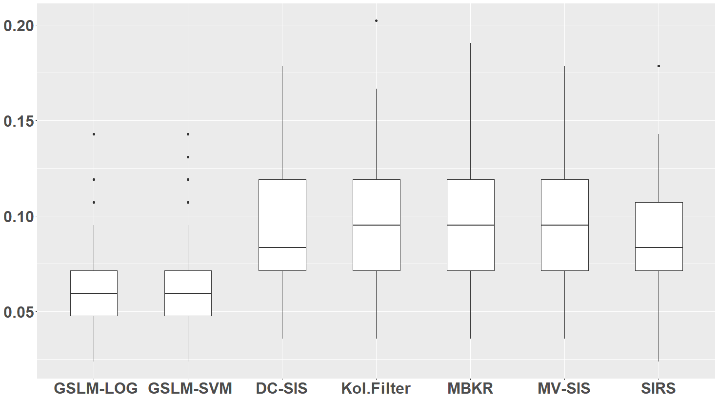
It is clear that both the averaged testing error and the false negative rate based on the selected sets of GSLM-LOG are the smallest among all the methods, and followed by GSLM-SVM. Note that the GSLM-LOG selects 26 genes and the GSLM-SVM selects 10 genes while the other screening based method select 36 genes. This implies that the proposed method has probably identified some important genes missed by the existing methods.

7 Discussion

It is known that continuous functions can be well approximated by those functions of the RKHS induced by some universal kernels under the infinity norm. We thus propose a general structure learning framework within the induced RKHS, which can be used to solve many interesting statistical problems, such as sparse learning, interaction selection, model identification and so on. The proposed framework is inspired by the fact that gradient functions can be employed to define the underlying structures of true target function without model specifications, and the nice properties of the RKHS facilitate the whole computation of the proposed framework. It is methodologically simple and computationally easy to implement, and can efficiently process large datasets. More importantly, it attains many advantages that it works for a general family of loss functions, and admits general dependence structures with theoretical guarantees under weaker conditions than existing methods. In our future work, we may extend current work to more complicated cases such as manifold learning and graph estimation.

Supplementary Material

Due to the space limit, additional numerical results and all the technical proofs of Theorems 1–5 are deferred to the Supplementary Material.

References

- Barber and Cands (2015) R. Barber and E. Cands. Controlling the false discovery rate via knockoffs. Annals of Statistics, 43:2055–2085, 2015.
- Boyd and Vandenberghe (2004) S. Boyd and L. Vandenberghe. Convex Optimization. Cambridge University Press, 2004.
- Corrêa et al. (2017) S. Corrêa, C. Panis, R. Binato, A. Herrera, L. Pizzatti, and E. Abdelhay. Identifying potential markers in breast cancer subtypes using plasma label-free proteomics. Journal of Proteomics, 151:33–42, 2017.
- Cui et al. (2015) H. Cui, R. Li, and W. Zhong. Model-free feature screening for ultrahigh dimensional discriminant analysis. Journal of the American Statistical Association, 110:630–641, 2015.
- Dasgupta et al. (2019) S. Dasgupta, Y. Goldberg, and M Kosorok. Feature elimination in kernel machines in moderately high dimensions. Annals of Statistics, 47:497–526, 2019.
- Dong and Wu (2021) Y. Dong and Y. Wu. Nonparametric interaction selection. Statistica Sinica, In press:1–37, 2021.
- Eberts and Steinwart (2013) M. Eberts and I. Steinwart. Optimal regression rates for svms using gaussian kernels. Electronic Journal of Statistics, 7:1–42, 2013.
- Fan and Lv (2008) J. Fan and J. Lv. Sure independence screening for ultrahigh dimensional feature space (with discussion). Journal of the Royal Statistical Society, Series B, 70:849–911, 2008.
- Fan and Lv (2010) J. Fan and J. Lv. A selective overview of variable selection in high dimensional feature space (invited review article). Statistica Sinica, 20:101–148, 2010.
- Fan et al. (2011) J. Fan, F. Yang, and R. Song. Nonparametric independence screening in sparse ultrahigh dimensional additive models. Journal of the American Statistical Association, 106:544–557, 2011.
- Fischer and Steinwart (2020) S. Fischer and I. Steinwart. Sobolev norm learning rates for regularized least-squares algorithms. Journal of Machine Learning Research, 21:1–38, 2020.
- Fu et al. (2020) A. Fu, B. Narasimhan, and S. Boyd. CVXR: An R package for disciplined convex optimization. Journal of Statistical Software, 94:1–34, 2020. doi: 10.18637/jss.v094.i14.
- Han (2019) X. Han. Nonparametric screening under conditional strictly convex loss for ultrahigh dimensional sparse data. Annals of Statistics, 47:1995–2022, 2019.
- Hang and Steinwart (2018) H. Hang and I. Steinwart. A bernstein-type inequality for some mixing processes and dynamical systems with an application to learning. Annals of Statistics, 45:708–743, 2018.
- Hao and Zhang (2014) N. Hao and H. Zhang. Interaction screening for ultra-high dimensional data. Journal of the American Statistical Association, 109:1285–1301, 2014.
- Hao et al. (2018) N. Hao, Y. Feng, and H. Zhang. Model selection for high dimensional quadratic regression via regularization. Journal of the American Statistical Association, 113:615–625, 2018.
- He and Wang (2020) X. He and J. Wang. Discovering model structure for partially linear models. Annals of the Institute of Statistical Mathematics, 72:45–63, 2020.
- He et al. (2013) X. He, L. Wang, and H. Hong. Quantile-adaptive model-free variable screening for high-dimensional heterogeneous data. Annals of Statistics, 41:342–369, 2013.
- He et al. (2020) X. He, S. Lv, and J. Wang. Variable selection for classification with derivative-induced regularization. Statistica Sinica, 30:2075–2103, 2020.
- He et al. (2021) X. He, J. Wang, and S. Lv. Efficient kernel-based variable selection with sparsistency. Statistica Sinica, In press:1–55, 2021.
- Huang et al. (2010) J. Huang, J. Horowitz, and F. Wei. Variable selection in nonparametric additive models. Annals of Statistics, 38:2282–2313, 2010.
- Kong et al. (2017) Y. Kong, D. Li, Y. Fan, and J. Lv. Interaction pursuit in high-dimensional multi-response regression via distance correlation. Annals of Statistics, 45:897–922, 2017.
- Li et al. (2012) R. Li, W. Zhong, and L. Zhu. Feature screening via distance correlation learning. Journal of the American Statistical Association, 107:1129–1139, 2012.
- Li and Liu (2019) Y. Li and J. Liu. Robust variable and interaction selection for logistic regression and general index models. Journal of the American Statistical Association, 114:271–286, 2019.
- Lian et al. (2015) H. Lian, H. Liang, and D. Ruppert. Separation of covariates into nonparametric and parametric parts in high-dimensional partially linear additive models. Statistica Sinica, 25:591–607, 2015.
- Lin and Zhang (2006) Y. Lin and H. Zhang. Component selection and smoothing in multivariate nonparametric regression. Annal of Statistics, 34:2272–2297, 2006.
- Liu et al. (2019) J. Liu, J. Liu, and X. Lu. Hoxa1 upregulation is associated with poor prognosis and tumor progression in breast cancer. Experimental and therapeutic medicine, 17:1896–1902, 2019.
- Liu et al. (2017) Y. Liu, J. Li, J. Zhang, Z. Yu, S. Yu, L. Wu, Y. Wang, X. Gong, C. Wu, X. Cai, L. Mo, M. Wang, J. Gu, and L. Chen. Oncogenic protein kinase d3 regulating networks in invasive breast cancer. International journal of biological sciences, 13:748–758, 2017.
- Loh (2017) P. Loh. Statistical consistency and asymptotic normality for high-dimensional robust m-estimators. Annals of Statistics, 45:866–896, 2017.
- Lv et al. (2018) S. Lv, H. Lin, H. Lian, and J. Huang. Oracle inequalities for sparse additive quantile regression in reproducing kernel Hilbert space. Annals of Statistics, 2:781–813, 2018.
- Ma et al. (2017) S. Ma, R. Li, and C Tsai. Variable screening via quantile partial correlation. Journal of the American Statistical Association, 112:650–663, 2017.
- Mai and Zou (2013) Q. Mai and H. Zou. The Kolmogorov filter for variable screening in high-dimensional binary classification. Biometrika, 100:229–234, 2013.
- Mendelson and Neeman (2010) S. Mendelson and J. Neeman. Regularization in kernel learning. Annal of Statistics, 38:526–565, 2010.
- Pan et al. (2019) W. Pan, X. Wang, W. Xiao, and H. Zhu. A generic sure independence screening procedure. Journal of the American Statistical Association, 114(526):928–937, 2019.
- Radchenko and James (2010) P. Radchenko and G. James. Variable selection using adaptive nonlinear interaction structures in high dimensions. Journal of the American Statistical Association, 105:1541–1553, 2010.
- Ritchie et al. (2001) M. Ritchie, L. Hahn, N. Roodi, L. Bailey, W. Dupont, F. Parl, and J. Moore. Multifactor-dimensionality reduction reveals high-order interactions among estrogen-metabolism genes in sporadic breast cancer. The American Journal of Human Genetics, 69:138–147, 2001.
- Rosasco et al. (2013) L. Rosasco, S. Villa, S. Mosci, M. Santoro, and A. Verri. Nonparametric sparsity and regularization. Journal of Machine Learning Research, 14:1665–1714, 2013.
- Shi et al. (2018) Y. Shi, Y. Zhao, Y. Zhang, N. AiErken, N. Shao, Y. Ye, R..and Lin, and S. Wang. TNNT1 facilitates proliferation of breast cancer cells by promoting G1/S phase transition. Life Sciences, 208:161–166, 2018.
- Simon-Gabriel and Schölkopf (2018) C. Simon-Gabriel and B. Schölkopf. Kernel distribution embeddings: Universal kernels, characteristic kernels and kernel metrics on distributions. Journal of Machine Learning Research, 19:1–29, 2018.
- Steinwart (2005) I. Steinwart. Consistency of support vector machines and other regularized kernel classifiers. IEEE Transactions on Information Theory, 51:128–142, 2005.
- Steinwart and Christmann (2008a) I. Steinwart and A. Christmann. Support Vector Machine. Springer, 2008a.
- Steinwart and Christmann (2008b) I. Steinwart and A. Christmann. Sparsity of svms that use the epsilon-insensitive loss. Advances in Neural Information Processing Systems, 21:1569–1576, 2008b.
- Sun et al. (2013) W. Sun, J. Wang, and Y. Fang. Consistent selection of tuning parameters via variable selection stability. Journal of Machine Learning Research, 14:3419–3440, 2013.
- Takeuchi et al. (2006) I. Takeuchi, Q. Le, T. Sears, and A. Smola. Nonparametric quantile estimation. Journal of Machine Learning Research, 7:1231–1264, 2006.
- Tang et al. (2021) X. Tang, F. Xue, and A. Qu. Individualized multidirectional variable selection. Journal of the American Statistical Association, In press, 2021.
- Wahba (MIT Press, 1998) G. Wahba. Support vector machines, reproducing kernel Hilbert spaces, and randomized GACV. Advances in kernel methods: support vector learning, pages 69–88, MIT Press, 1998.
- Wang and Leng (2016) X. Wang and C. Leng. High dimensional ordinary least squares projection for screening variables. Journal of the Royal Statistical Society, Series B, 78:589–611, 2016.
- Wu and Liu (2009) Y. Wu and Y. Liu. Variable selection in quantile regression. Statistica Sinica, 19:801–817, 2009.
- Yang et al. (2016) L. Yang, S. Lv, and J. Wang. Model-free variable selection in reproducing kernel Hilbert space. Journal of Machine Learning Research, 17:1–24, 2016.
- Zhang et al. (2016a) C. Zhang, Y. Liu, and Y. Wu. On quantile regression in reproducing kernel Hilbert spaces with data sparsity constraint. Journal of Machine Learning Research, 17:1–45, 2016a.
- Zhang et al. (2011) H. Zhang, G. Cheng, and Y. Liu. Linear or nonlinear? automatic structure discovery for partially linear models. Journal of the American Statistical Association, 106:1099–1112, 2011.
- Zhang et al. (2016b) X. Zhang, Y. Wu, L. Wang, and R. Li. Variable selection for support vector machines in moderately high dimensions. Journal of the Royal Statistical Society Series B, 78:53–76, 2016b.
- Zhou (2007) D. Zhou. Derivative reproducing properties for kernel methods in learning theory. Journal of Computational and Applied Mathematics, 220:456–463, 2007.
- Zhou and Zhu (2018) Y. Zhou and L. Zhu. Model-free feature screening for ultrahigh dimensional data through a modified Blum-Kiefer-Rosenblatt correlation. Statistica Sinica, 28:1351–1370, 2018.
- Zhu and Hastie (2005) J. Zhu and T. Hastie. Kernel logistic regression and the import vector machine. Journal of Computational and Graphical Statistics, 14:185–205, 2005.
- Zhu et al. (2011) L. Zhu, L. Li, R. Li, and L. Zhu. Model-free feature screening for ultrahigh-dimensional data. Journal of the American Statistical Association, 106:1464–1475, 2011.