Discrete-Continuous Mixtures in Probabilistic Programming:
Generalized Semantics and Inference Algorithms
Supplementary Materials

Abstract

Despite the recent successes of probabilistic programming languages (PPLs) in AI applications, PPLs offer only limited support for random variables whose distributions combine discrete and continuous elements. We develop the notion of measure-theoretic Bayesian networks (MTBNs) and use it to provide more general semantics for PPLs with arbitrarily many random variables defined over arbitrary measure spaces. We develop two new general sampling algorithms that are provably correct under the MTBN framework: the lexicographic likelihood weighting (LLW) for general MTBNs and the lexicographic particle filter (LPF), a specialized algorithm for state-space models. We further integrate MTBNs into a widely used PPL system, BLOG, and verify the effectiveness of the new inference algorithms through representative examples.

1 Introduction

As originally defined by Pearl (1988), Bayesian networks express joint distributions over finite sets of random variables as products of conditional distributions. Probabilistic programming languages (PPLs) (Koller et al., 1997; Milch et al., 2005a; Goodman et al., 2008; Wood et al., 2014b) apply the same idea to potentially infinite sets of variables with general dependency structures. Thanks to their expressive power, PPLs have been used to solve many real-world applications, including Captcha (Le et al., 2017), seismic monitoring (Arora et al., 2013), 3D pose estimation (Kulkarni et al., 2015), generating design suggestions (Ritchie et al., 2015), concept learning (Lake et al., 2015), and cognitive science applications (Stuhlmüller & Goodman, 2014).

In practical applications, we often have to deal with a mixture of continuous and discrete random variables. Existing PPLs support both discrete and continuous random variables, but not discrete-continuous mixtures, i.e., variables whose distributions combine discrete and continuous elements. Such variables are fairly common in practical applications: sensors that have thresholded limits, e.g. thermometers, weighing scales, speedometers, pressure gauges; or a hybrid sensor that can report a either real value or an error condition. The occurrence of such variables has been noted in many other applications from a wide range of scientific domains (Kharchenko et al., 2014; Pierson & Yau, 2015; Gao et al., 2017).

Many PPLs have a restricted syntax that forces the expressed random variables to be either discrete or continuous, including WebPPL (Goodman & Stuhlmüller, 2014), Edward (Tran et al., 2016), Figaro (Pfeffer, 2009) and Stan (Carpenter et al., 2016). Even for PPLs whose syntax allows for mixtures of discrete and continuous variables, such as BLOG (Milch et al., 2005a), Church (Goodman, 2013), Venture (Mansinghka et al., 2014) and Anglican (Wood et al., 2014a), the underlying semantics of these PPLs implicitly assumes the random variables are not mixtures. Moreover, the inference algorithms associated with the semantics inherit the same assumption and can produce incorrect results when discrete-continuous mixtures are used.

Consider the following GPA example: a two-variable Bayes net $\emph{Nationality}\rightarrow\emph{GPA}$ where the nationality follows a binary distribution

$$P(\emph{Nationality}=\emph{USA})=P(\emph{Nationality}=\emph{India})=0.5\vskip-3.99994pt$$

and the conditional probabilities are discrete-continuous mixtures

$$\emph{GPA}|\emph{Nationality}=\emph{USA}$$

$$\sim 0.01\cdot\mathbf{1}\left\{\emph{GPA}=4\right\}+0.99\cdot\text{ Unif}(0,4),$$

$$\emph{GPA}|\emph{Nationality}=\emph{India}$$

$$\sim 0.01\cdot\mathbf{1}\left\{\emph{GPA}=10\right\}+0.99\cdot\text{ Unif}(0,10).$$

This is a typical scenario in practice because many top students have perfect GPAs. Now suppose we observe a student with a GPA of 4.0. Where do they come from? If the student is Indian, the probability of any singleton set $\{g\}$ where $0<g<10$ is zero, as this range has a probability density. On the other hand if the student is American, the set $\{4\}$ has the probability $0.01$. Thus, by Bayes theorem, $P(\emph{Nationality}=\emph{USA}|\emph{GPA}=4)=1$, which means the student must be from the USA.

However, if we run the default Bayesian inference algorithm for this problem in PPLs, e.g., the standard importance sampling algorithm (Milch et al., 2005b), a sample that picks India receives a density weight of $0.99/10.0=0.099$, whereas one that picks USA receives a discrete-mass weight of $0.01$. Since the algorithm does not distinguish probability density and mass, it will conclude that the student is very probably from India, which is far from the truth.

We can fix the GPA example by considering a density weight infinitely smaller than a discrete-mass weight (Nitti et al., 2016; Tolpin et al., 2016). However, the situation becomes more complicated when involving more than one evidence variable, e.g., GPAs over multiple semesters for students who may study in both countries. Vector-valued variables also cause problems—does a point mass in three dimensions count more or less than a point mass in two dimensions? These practical issues motivate the following two tasks:

• Inherit all the existing properties of PPL semantics and extend it to handle random variables with mixed discrete and continuous distributions;

• Design provably correct inference algorithms for the extended semantics.

In this paper, we carry out all these two tasks and implement the extended semantics as well as the new algorithms in a widely used PPL, Bayesian Logic (BLOG) (Milch et al., 2005a).

1.1 Main Contributions

Measure-Theoretical Bayesian Nets (MTBNs)

Measure theory can be applied to handle discrete-continuous mixtures or even more abstract measures. In this paper, we define a generalization of Bayesian networks called measure-theoretic Bayesian networks (MTBNs) and prove that every MTBN represents a unique measure on the input space. We then show how MTBNs can provide a more general semantic foundation for PPLs.

More concretely, MTBNs support (1) random variables with infinitely (even uncountably) many parents, (2) random variables valued in arbitrary measure spaces (with $\mathbb{R}^{N}$ as one case) distributed according to any measure (including discrete, continuous and mixed), (3) establishment of conditional independencies implied by an infinite graph, and (4) open-universe semantics in terms of the possible worlds in the vocabulary of the model.

Inference Algorithms

We propose a provably correct inference algorithm, lexicographic likelihood weighting (LLW), for general MTBNs with discrete-continuous mixtures. In addition, we propose LPF, a particle-filtering variant of LLW for sequential Monte Carlo (SMC) inference on state-space models.

Incorporating MTBNs into an existing PPL

We incorporate MTBNs into BLOG with simple modifications and then define the generalized BLOG language, measure-theoretic BLOG, which formally supports arbitrary distributions, including discrete-continuous mixtures. We prove that every generalized BLOG model corresponds to a unique MTBN. Thus, all the desired theoretical properties of MTBNs can be carried to measure-theoretic BLOG. We also implement the LLW and LPF algorithms in the backend of measure-theoretic BLOG and use three representative examples to show their effectiveness.

1.2 Organization

This paper is organized as follows. We first discuss related work in Section 2. In Section 3, we formally define measure-theoretic Bayesian nets and study their theoretical properties. Section 4 describes the LLW and LPF inference algorithms for MTBNs with discrete-continuous mixtures and establishes their correctness. In Section 5, we introduce the measure-theoretic extension of BLOG and study its theoretical foundations for defining probabilistic models. In Section 6, we empirically validate the generalized BLOG system and the new inference algorithms on three representative examples.

2 Related Work

The motivating GPA example has been also discussed as a special case under some other PPL systems (Tolpin et al., 2016; Nitti et al., 2016). Tolpin et al. (2016) and Nitti et al. (2016) proposed different specialized tricks to derive the correct answer particularly for the GPA example but did not provide any general correctness guarantees. While the MTBN framework is much more general and the LLW and LPF algorithms are provably correct.

The closest related work to our framework is by Milch (2006), who utilize a supportive numbering of random variables, implying that each random variable has finitely many consistent parents. In addition, they only handle random variables with countably infinite ranges. The BLP framework presented by Kersting & De Raedt (2007) unifies logic programming with probability models, but requires each random variable to be influenced by a finite set of random variables in order to define the semantics. This amounts to requiring only finitely many ancestors of each node. Choi et al. (2010) present an algorithm for carrying out lifted inference over models with purely continuous random variables. They also require parfactors to be functions over finitely many random variables, thus limiting the set of influencing variables for each node to be finite. Gutmann et al. (2011a) also define densities over finite dimensional vectors. In a relatively more general formulation (Gutmann et al., 2011b) define the distribution of each random variable using a definite clause, which corresponds to the limitation that each random variable (either discrete or continuous) has finitely many parents. Frameworks building on Markov networks also have similar restrictions. Wang & Domingos (2008) only consider networks of finitely many random variables, which can have either discrete or continuous distributions. Singla & Domingos (2007) extend Markov logic to infinite (non-hybrid) domains, provided that each random variable has only finitely many influencing random variables.

In contrast, our approach not only allows models with arbitrarily many random variables with mixed discrete and continuous distributions, but each random variable can also have arbitrarily many parents as long as all ancestor chains are finite (but unbounded). The presented work constitutes a rigorous framework for expressing probability models with the broadest range of cardinalities (uncountably infinite parent sets) and nature of random variables (discrete, mixed, and even arbitrary measure spaces), with clear semantics in terms of first-order possible worlds and the generalization of conditional independences on such models.

Lastly, there are also other works using measure-theoretic approaches to analyze the semantics properties of probabilistic programs but with different emphases (Shan & Ramsey, 2017; Staton, 2017; Ramsey, 2016).

3 Measure-Theoretic Bayesian Networks

In this section, we introduce measure-theoretic Bayesian nets (MTBNs) and prove that a MTBN represents a unique measure with desired theoretical properties. We assume familiarity with measure-theoretic approaches to probability theory. Some background is included in Appx. A.

We begin with some necessary definitions of graph theory.

Definition 3.1.

A digraph $G$ is a pair $G=(V,E)$ of a set of vertices $V$, of any cardinality, and a set of directed edges $E\subseteq V\times V$. Write $u\rightarrow v$ if $(u,v)\in E$, and $u\mapsto v$ if there is a path from $u$ to $v$ in $G$.

Definition 3.2.

A vertex $v\in V$ is a root vertex if there are no incoming edges to it, i.e., no $u\in V$ such that $u\rightarrow v$. Let ${\rm pa}(v)=\{u\in V:u\rightarrow v\}$ denote the set of parents of a vertex $v\in V$, and ${\rm nd}(v)=\{u\in V:\text{not }v\mapsto u\}$ denote its set of non-descendants.

Definition 3.3.

A well-founded digraph $(V,E)$ is one with no countably infinite ancestor chain $v_{0}\leftarrow v_{1}\leftarrow v_{2}\leftarrow\dots$.

This is the natural generalization of a finite directed acyclic graph to the infinite case. Now we are ready to give the key definition of this paper.

Definition 3.4.

A measure-theoretic Bayesian network $M=(V,E,\{\mathcal{X}_{v}\}_{v\in V},\{K_{v}\}_{v\in V})$ consists of (a) a well-founded digraph $(V,E)$ of any cardinality, (b) an arbitrary measurable space $\mathcal{X}_{v}$ for each $v\in V$, and (c) a probability kernel $K_{v}$ from $\prod_{u\in{\rm pa}(v)}\mathcal{X}_{u}$ to $\mathcal{X}_{v}$ for each $v\in V$.

By definition, MTBNs allow us to define very general and abstract models with the following two major benefits:

1. We can define random variables with infinitely (even uncountably) many parents because MTBN is defined on a well-founded digraph.

2. We can define random variables in arbitrary measure spaces (with $\mathbb{R}^{N}$ as one case) distributed according to any measure (including discrete, continuous and mixed).

Next, we related MTBN to a probability measure. Fix an MTBN $M=(V,E,\{\mathcal{X}_{v}\}_{v\in V},\{K_{v}\}_{v\in V})$. For $U\subseteq V$ let $\mathcal{X}_{U}=\prod_{u\in U}\mathcal{X}_{u}$ be the product measurable space over variables $u\in U$. With this notation, $K_{v}$ is a kernel from $\mathcal{X}_{{\rm pa}(v)}$ to $\mathcal{X}_{v}$. Whenever $W\subseteq U$ let $\pi^{U}_{W}\colon\mathcal{X}_{U}\to\mathcal{X}_{W}$ denote the projection map. Let $\mathcal{X}_{V}$ be our base measurable space upon which we will consider different probability measures $\mu$. Let $X_{v}$ for $v\in V$ denote both the underlying set of $\mathcal{X}_{v}$ and the random variable given by the projection $\pi^{V}_{\{v\}}$, and $X_{U}$ for $U\subseteq V$ the underlying space of $X_{U}$ and the random variable given by the projection $\pi^{V}_{U}$.

Definition 3.5.

A MTBN $M$ represents a measure $\mu$ on $\mathcal{X}_{V}$, if for all $v\in V$:

• $X_{v}$ is conditionally independent of its non-descendants $X_{{\rm nd}(v)}$ given its parents $X_{{\rm pa}(v)}$.

• $K_{v}(X_{{\rm pa}(v)},A)=\mathop{\mathbb{P}}_{\mu}[X_{v}\in A|X_{{\rm pa}(v)}]$ holds almost surely for any $A\in\mathcal{X}_{v}$, i.e., $K_{v}$ is a version of the conditional distribution of $X_{v}$ given its parents.

Def. 3.5 captures the generalization of the local properties of Bayes Nets – conditional independence and conditional distributions defined by parent-child relationships. Here we implicit assume the conditional probability exists and is unique. This is a mild condition because this holds as long as the probability space is regular (Kallenberg, 2002).

The next theorem shows our definition of MTBN is proper.

Theorem 3.6.

A MTBN $M$ represents a unique measure $\mu$ on $\mathcal{X}_{V}$.

Theorem 3.6 lays out the foundation of MTBN. Its proof requires a series of intermediate results. We first define a projective family of measures. This gives a way to recursively construct our measure $\mu$. We then define a notion of consistency such that every consistent projective family constructs a measure that $M$ represents. Lastly, we give an explicit characterization of the unique consistent projective family, and thus of the unique measure $M$ represents. The full proof is in Appx. B.

4 Generalized Inference Algorithms

We introduce the lexicographic likelihood weighting (LLW) algorithm for provably correct inference on MTBNs. We also present lexicographic particle filter (LPF) for state-space models by adapting LLW into the SMC framework.

4.1 Lexicographic likelihood weighting

Suppose we have a MTBN with finitely many random variables $X_{1},\dots,X_{N}$, and that, without loss of generality, we observe real-valued random variables $X_{1},\dots,X_{M}$ for $M<N$ as evidence. Suppose the distribution of $X_{i}$ given its parents $X_{{\rm pa}(i)}$ is a mixture between a density $f_{i}(x_{i}|x_{{\rm pa}(i)})$ with respect to Lebesgue and a discrete distribution $F_{i}(x_{i}|x_{{\rm pa}(i)})$, i.e., for any $\epsilon>0$, we have $P(X_{i}\in[x_{i}-\epsilon,x_{i}]|X_{{\rm pa}(i)})=\sum_{x\in[x_{i}-\epsilon,x_{i}]}F_{i}(x_{i}|X_{{\rm pa}(i)})+\int_{x_{i}-\epsilon}^{x_{i}}f_{i}(x|X_{{\rm pa}(i)})\,dx.$ Note this implies $F_{i}(x_{i}|x_{{\rm pa}(i)})$ is nonzero for at most countably many values $x_{i}$. If $F_{i}$ is nonzero for finitely many points, it can be represented by a list of those points and their values.

Lexicographic Likelihood Weighting (LLW) extends the classical likelihood weighting (Milch et al., 2005b) to this setting. It visits each node of the graph in topological order, sampling those variables that are not observed, and accumulating a weight for those that are observed. In particular, at an evidence variable $X_{i}$ we update a tuple $(d,w)$ of the number of densities and a weight, initially $(0,1)$, by:

$$(d,w)\leftarrow\begin{cases}(d,wF_{i}(x_{i}|x_{{\rm pa}(i)}))&F_{i}(x_{i}|x_{{\rm pa}(i)})>0,\\ (d+1,wf_{i}(x_{i}|x_{{\rm pa}(i)}))&\text{otherwise.}\end{cases}$$ (1)

Finally, having $K$ samples $x^{(1)},\dots,x^{(K)}$ by this process and accordingly a tuple $(d^{(i)},w^{(i)})$ for each sample $x^{(i)}$, let $d^{*}=\min_{i:w^{(i)}\neq 0}d^{(i)}$ and estimate $E[f(X)|X_{1:M}]$ by

$$\frac{\sum_{\{i:d^{(i)}=d^{*}\}}w^{(i)}\,f(x^{(i)})}{\sum_{\{i:d^{(i)}=d^{*}\}}w^{(i)}}.$$ (2)

The algorithm is summarised in Alg. 1 The next theorem shows this procedure is consistent.

Theorem 4.1.

LLW is consistent: (2) converges almost surely to $\mathop{\mathbb{E}}[f(X)|X_{1:M}]$.

Algorithm 1 Lexicographic Likelihood Weighting

0:  densities $f$, masses $F$, evidences $E$, and $K$.

 for $i=1\ldots K$ do

  sample all the ancestors of $E$ from prior

  compute $(d^{(i)},w^{(i)})$ by Eq. (1)

 end for

 $d^{\star}\leftarrow\min_{i:w^{(i)}\neq 0}d^{(i)}$

 Return $\left(\sum_{i:d^{(i)}=d^{\star}}w^{(i)}f(x^{(i)})\right)/\left(\sum_{i:d^{(i)}=d^{\star}}w^{(i)}\right)$

In order to prove Theorem 4.1, the main technique we adopt is to use a more restricted algorithm, the Iterative Refinement Likelihood Weighting (IRLW) as a reference.

4.1.1 Iterative refinement likelihood weighting

Suppose we want to approximate the posterior distribution of an $\mathcal{X}$-valued random variable $X$ conditional on a $\mathcal{Y}$-valued random variable $Y$, for arbitrary measure spaces $\mathcal{X}$ and $\mathcal{Y}$. In general, there is no notion of a probability density of $Y$ given $X$ for which to weight samples. If, however, we could make a discrete approximation $Y_{t}$ of $Y$ then we could weight samples by the probability $P[Y_{t}=y_{t}|X]$. If we increase the accuracy of the approximation with the number of samples, this should converge in the limit. We show this is possible, if we are careful about how we approximate:

Definition 4.2.

An approximation scheme for a measurable space $\mathcal{Y}$ consists of a measurable space $\mathcal{A}$ and measurable approximation functions $\alpha_{i}\colon\mathcal{Y}\to\mathcal{A}$ for $i=1,2,\dots$ and $\alpha^{j}_{i}\colon\mathcal{A}\to\mathcal{A}$ for $i<j$ such that $\alpha_{j}\circ\alpha^{j}_{i}=\alpha_{i}$ and $y$ can be measurably recovered from the subsequence $\alpha_{t}(y),\alpha_{t+1}(y),\dots$ for any $t>0$.

When $Y$ is a real-valued variable we will use the approximation scheme $\alpha_{n}(y)=2^{-n}\lceil 2^{n}y\rceil$ where $\lceil r\rceil$ denotes the ceiling of $r$, i.e., the smallest integer no smaller than it. Observe in this case that $P(\alpha_{n}(Y)=\alpha_{n}(y))=P(\alpha_{n}(y)-2^{-n}<Y\leq\alpha_{n}(y))$ which we can compute from the CDF of $Y$.

Lemma 4.3.

If $X,Y$ are real-valued random variables with $\mathop{\mathbb{E}}|X|<\infty$, then $\lim_{i\to\infty}\mathop{\mathbb{E}}[X|\alpha_{i}(Y)]=\mathop{\mathbb{E}}[X|Y]$.

Proof.

Let $\mathcal{F}_{i}=\sigma(\alpha_{i}(Y))$ be the sigma algebra generated by $\alpha_{i}(Y)$. Whenever $i\leq j$ we have $\alpha_{i}(Y)=(\alpha_{j}\circ\alpha^{j}_{i})(Y)$ and so $\mathcal{F}_{i}\subseteq\mathcal{F}_{j}$. This means $\mathop{\mathbb{E}}[X|\alpha_{i}(Y)]=\mathop{\mathbb{E}}[X|\mathcal{F}_{i}]$ is a martingale, so we can use martingale convergence results. In particular, since $\mathop{\mathbb{E}}|X|<\infty$

$$\mathop{\mathbb{E}}[X|\mathcal{F}_{i}]\to\mathop{\mathbb{E}}[X|\mathcal{F}_{\infty}]\hskip 10.00002pt\text{a.s.\ and in $L^{1}$},\vskip-5.0pt$$

where $\mathcal{F}_{\infty}=\bigcup_{i}\mathcal{F}_{i}$ is the sigma-algebra generated by $\{\alpha_{i}(Y):i\in\mathbb{N}\}$ (see Theorem 7.23 in (Kallenberg, 2002)).

$Y$ is a measurable function of the sequence $(\alpha_{1}(Y),\dots)$, as $\lim_{i\to\infty}\alpha_{i}(Y)=Y$, and so $\sigma(Y)\subseteq\mathcal{F}_{\infty}$. By definition the sequence is a measurable function of $Y$, and so $\mathcal{F}_{\infty}\subseteq\sigma(Y)$, and so $\mathop{\mathbb{E}}[X|\mathcal{F}_{\infty}]=\mathop{\mathbb{E}}[X|Y]$ giving our result. ∎

Iterative refinement likelihood weighting (IRLW) samples $x^{(1)},\dots,x^{(K)}$ from the prior and evaluates:

$$\frac{\sum_{i=1}^{K}P(\alpha_{n}(Y)|X=x^{(i)})f(x^{(i)})}{\sum_{i=1}^{K}P(\alpha_{n}(Y)|X=x^{(i)})}$$ (3)

Using Lemma 4.3, G.12, and G.13, we can show IRLW is consistent.

Theorem 4.4.

IRLW is consistent: (3) converges almost surely to $\mathop{\mathbb{E}}[f(X)|Y]$.

4.1.2 Proof of Theorem 4.1

Now we are ready to prove Theorem 4.1.

Proof of Theorem 4.1.

We only prove where the evidence variables are leaves. It is straightforward to extend the proof when the evidence variables are non-leaf nodes. Let $x$ be a sample produced by the algorithm with number of densities and weight $(d,w)$. With $I_{n}=\prod_{i=1\ldots M}(\alpha_{n}(x_{i})-2^{-n},\alpha_{n}(x_{i})]$ a $2^{-n}$-cube around $x_{1:M}$ we have

$$\lim_{n\to\infty}\frac{P(X_{1:M}\in I_{n}|X_{M+1:N}=x_{M+1:N})}{w\,2^{-dn}}=1.$$

Using $I_{n}$ as an approximation scheme by Def. 4.2, the numerator in the above limit is the weight used by IRLW. But given the above limit, using $w\,2^{-dn}$ as the weight will give the same result in the limit. Then if we have $K$ samples, in the limit of $n\to\infty$ only those samples $x^{(i)}$ with minimal $d^{(i)}$ will contribute to the estimation, and up to normalization they will contribute weight $w^{(i)}$ to the estimation. ∎

4.2 Lexicographic particle filter

Likelihood weighting based algorithms suffer from curse of dimensionality. One important class of models with high dimensionality are state-space models. A state-space model (SSM) consists of latent states $\left\{X_{t}\right\}_{0\leq t\leq T}$ and the observations $\left\{Y_{t}\right\}_{0\leq t\leq T}$ with a special dependency structure where ${\rm pa}(Y_{t})=X_{t}$ and ${\rm pa}(X_{t})=X_{t-1}$ for $0<t\leq T$.

Sequential Monte Carlo (SMC) (Doucet et al., 2001), i.e., particle filer, is a widely adopted class of methods for inference on SSMs. Given the observed variables $\{Y_{t}\}_{0\leq t\leq T}$, the posterior distribution $P(X_{t}|Y_{0:t})$ is approximated by a set of $K$ particles where each particle $x_{t}^{(k)}$ represents a sample of $\{X_{i}\}_{0\leq i\leq t}$. Particles are propagated forward through the transition model $P(X_{t}|X_{t-1})$ and resampled at each time step $t$ according to the weight of each particle, which is defined by the likelihood of observation $Y_{t}$.

In the MTBN setting, the distribution of $Y_{t}$ given its parent $X_{t}$ can be a mixture of density $f_{t}(y_{t}|x_{t})$ and a discrete distribution $F_{t}(y_{t}|x_{t})$. Hence, the resampling step in particle filter should be accordingly modified: following the idea from LLW, when computing the weight of a particle, we enumerate all the observations $y_{t,i}$ at time step $t$ and again update a tuple $(d,w)$, initially (0,1), by

$$(d,w)\leftarrow\begin{cases}(d,wF_{t}(y_{t,i}|x_{t}))&\text{ $F_{t}(y_{t,i}|x_{t})>0$,}\\ (d+1,wf_{t}(y_{t,i}|x_{t}))&\text{otherwise.}\end{cases}$$ (4)

We discard all those particles with a non-minimum $d$ value and then perform the normal resampling step. We call this algorithm lexicographical particle filter (LPF), which is summarized in Alg. 2.

Algorithm 2 Lexicographic Particle Filter (LPF)

0:  densities $f$, masses $F$, evidences $Y$, and $K$

 for $t=0,\ldots,T$ do

  for $k=0,\ldots,K$ do

   $x_{t}^{(k)}\leftarrow$ sample from transition

   compute $(d^{(k)},w^{(k)})$ by Eq. 4

  end for

  $d^{\star}\leftarrow\min_{k:w^{(k)}\neq 0}d^{(k)}$

  $\forall k:d^{(k)}>d^{\star}$, $w^{(k)}\leftarrow 0$

  Output $\left(w^{(k)}f(x_{t}^{(k)})\right)/\left(\sum_{k}w^{(k)}\right)$

  resample particles according to $w^{(k)}$

 end for

The following theorem guarantees the correctness of LPF. Its Proof easily follows the analysis for LLW and classical proof from importance sampling to particle filter.

Theorem 4.5.

LPF is consistent: the outputs of Alg. 2 converges almost surely to $\{E[f(X_{t})|Y_{0:t}]\}_{0\leq t\leq T}$.

5 Generalized Probabilistic Programming Languages

In Section 3 and Section 4 we provided the theoretical foundation of MTBN and general inference algorithms. This section describes how to incorporate MTBN into a practical PPL. Here our focus is a widely used open-universe PPL, BLOG (Milch, 2006). We define the generalized BLOG language, the measure-theoretic BLOG, and prove that every well-formed measure-theoretic BLOG model corresponds to a unique MTBN. Note that our approach also applies to other PPLs.

We begin with a brief description of the core syntax of BLOG, with particular emphasis on (1) the most important existing syntax for open-universe semantics, i.e., the number statement, and (2) a newly introduced syntax to accommodate MTBN, i.e., the Mix distribution. Further description of BLOG’s syntax can be found in Li & Russell (2013).

5.1 Syntax of measure-theoretic BLOG

1 Type Applicant, Country;
2 distinct Country NewZealand, India, USA;
3 #Applicant(Nationality = c) ~
4  if (c==USA) then Poisson(50)
5  else Poisson(5);
6 origin Country Nationality(Applicant);
7 random Real GPA(Applicant s) ~
8  if Nationality(s) == USA then
9      Mix({ TruncatedGauss(3, 1, 0, 4) -> 0.9998,
10          4 -> 0.0001, 0 -> 0.0001})
11 else Mix({ TruncatedGauss(5, 4, 0, 10) -> 0.989,
12           10 -> 0.009, 0 -> 0.002});
13 random Applicant David ~
14     UniformChoice({a for Applicant a});
15 obs GPA(David) = 4;
16 query Nationality(David) = USA;

Figure 1: A BLOG code for the GPA example.

Fig. 1 shows a BLOG model with measure-theoretic extensions for a multi-student GPA example. Line 1 declares two types, Applicant and Country. Line 2 defines 3 distinct countries with keyword distinct, New Zealand, India and USA. Line 3 to 5 defines a number statement, which states that the number of US applicants follows a Poisson distribution with a higher mean than those from New Zealand or India. Line 6 defines an origin function, which maps the object being generated to the arguments that were used in the number statement that was responsible for generating it. Here Nationality maps applicants to their nationalities. Line 7 and 13 define two random variables by keyword random. Line 7 to 12 states that the GPA of an applicant is distributed as a mixture of weighted discrete and continuous distributions. For US applicants, the range of values $0<\emph{GPA}<4$ follows a truncated Gaussian with bounds 0 and 4 (line 9). The probability mass outside the range is attributed to the corresponding bounds: $P(\emph{GPA}=0)=P(\emph{GPA}=4)=10^{-4}$ (lines 10). GPA distributions for other countries are specified similarly. Line 13 defines a random applicant $David$. Line 15 states that the David’s GPA is observed to be 4 and we query in line 16 whether David is from USA.

Number Statement (line 3 to 5)

$$\#\textrm{Type}_{i} (g_{1}=x_{1},\ldots,g_{k}=x_{k})\sim$$

$$\textrm{ }\textrm{if }\varphi_{1}(\bar{y}_{1})\textrm{ then }c_{1}(\bar{e}_{1})$$

$$\textrm{ }\textrm{else if }\varphi_{2}(\bar{y}_{2})\textrm{ then }c_{2}(\bar{e}_{2})$$

$$\textrm{ }\ldots$$

$$\textrm{ }\textrm{else }c_{m}(\bar{e}_{m});$$

Figure 2: Syntax of number statements

Fig. 2 shows the syntax of a number statement for $\emph{Type}_{i}$. In this specification, $g_{j}$ are origin functions (discussed below); $\bar{y}_{j}$ are tuples of arguments drawn from $\bar{x}=x_{1},\ldots,x_{k}$; $\varphi_{j}$ are first-order formulas with free variables $\bar{y}_{j}$; $\bar{e}_{j}$ are tuples of expressions over a subset of $x_{1},\ldots,x_{k}$; and $c_{j}(\bar{e}_{j})$ specify kernels $\kappa_{j}:\Pi_{\{\mathcal{X}_{\tau_{e}}:e\in\bar{e}_{j}\}}\mathcal{X}_{e}\rightarrow\mathbb{N}$ where $\tau_{e}$ is the type of the expression $e$.

The arguments $\bar{x}$ provided in a number statement allow one to utilize information about the rest of the model (and possibly other generated objects) while describing the number of objects that should be generated for each type. These assignments can be recovered using the origin functions $g_{j}$, each of which is declared as:

$$\mathtt{origin}~\textrm{Type}_{j}~~g_{j}(\textrm{Type}_{i}),\vskip-1.99997pt$$

where $Type_{j}$ is the type of the argument $x_{j}$ in the number statement of $Type_{i}$ where $g_{j}$ was used. The value of the $j^{th}$ variable used in the number statement that generated $u$, an element of the universe, is given by $g_{j}(u)$. Line 6 in Fig. 1 is an example of origin function.

Mixture Distribution (line 9 to 12)

In the measure-theoretic BLOG, we introduce a new distribution, the mixture distribution (e.g., lines 9-10 in Fig. 1). A mixture distribution is specified as:

$$\mathtt{Mix}(\{c_{1}(\bar{e}_{1})\rightarrow w_{1}(\bar{e}^{\prime}),\ldots,c_{k}(\bar{e}_{k})\rightarrow w_{k}(\bar{e}^{\prime})\}),\vskip-5.0pt$$

where $c_{i}$ are arbitrary distributions, and $w_{i}$’s are arbitrary real valued functions that sum to 1 for every possible assignment to their arguments: $\forall\bar{e}^{\prime}\sum_{i}w_{i}(\bar{e}^{\prime})=1$. Note that in our implementation of the measure-theoretical BLOG, we only allow Mix distribution to express a mixture of densities and masses for simplifying the system design, although it still possible to express the same semantics without Mix.

5.2 Semantics of measure-theoretic BLOG

In this section we study semantics of measure-theoretic BLOG and its theoretical properties. Every BLOG model implicitly defines a first-order vocabulary consisting of the set of functions and types mentioned in the model. BLOG’s semantics are based on the standard, open-universe semantics of first-order logic. We first define the set of all possible elements that may be generated for a BLOG model.

Definition 5.1.

The set of possible elements $\mathcal{U}_{\mathcal{M}}$ for a BLOG model $\mathcal{M}$ with types $\{\tau_{1},\ldots,\tau_{k}\}$ is $\bigcup_{j\in\mathbb{N}}\{\mathcal{U}_{j}\}$, where

• $\mathcal{U}_{0}=\langle U^{0}_{1},\ldots,U^{0}_{k}\rangle$, $U^{0}_{j}=\{c_{j}:c_{j}$ is a distinct $\tau_{i}$ constant in $\mathcal{M}\}$

• $\mathcal{U}_{i+1}=\langle U^{i+1}_{1},\ldots,U^{i+1}_{k}\rangle$, where $U^{i+1}_{m}=U^{i}_{m}\cup\{u_{\nu,\bar{u},m}:\nu(\bar{x})$ is a number statement of type $\tau_{m}$, $\bar{u}$ is a tuple of elements of the type of $\bar{x}$ from $\mathcal{U}^{i}$, $m\in\mathbb{N}\}$

Def. 5.1 allows us to define the set of random variables corresponding to a BLOG model.

Definition 5.2.

The set of basic random variables for a BLOG model $\mathcal{M}$, $BRV(\mathcal{M})$, consists of:

• for each number statement $\nu(\bar{x})$, a number variable $V_{\nu}[\bar{u}]$ over the standard measurable space $\mathbb{N}$, where $\bar{u}$ is of the type of $\bar{x}$.

• for each function $f(\bar{x})$ and tuple $\bar{u}$ from $\mathcal{U}_{\mathcal{M}}$ of the type of $\bar{x}$, a function application variable $V_{f}[\bar{u}]$ with the measurable space $\mathcal{X}_{V_{f}[\bar{u}]}=\mathcal{X}_{\tau_{f}}$, where $\mathcal{X}_{\tau_{f}}$ is the measurable space corresponding to $\tau_{f}$, the return type of $f$.

We now define the space of consistent assignments to random variables.

Definition 5.3.

An instantiation $\sigma$ of the basic RVs defined by a BLOG model $\mathcal{M}$ is consistent if and only if:

• For every element $u_{\nu,\bar{v},i}$ used in an assignment of the form $\sigma(V_{f}[\bar{u}])=w$ or $\sigma(V_{\nu}[\bar{u}])=m>0$, $\sigma(V_{\nu}[\bar{v}])\geq i$;

• For every fixed function symbol $f$ with the interpretation $\tilde{f}$, $\sigma(V_{f}[\bar{u}])=\tilde{f}(\bar{u})$; and

• For every element $u_{\nu,\bar{u}=\langle u_{1},\ldots,u_{m}\rangle,i}$, generated by the number statement $\nu$, with origin functions $g_{1},\ldots,g_{m}$, for every $g_{j}\in\{g_{1},\ldots,g_{m}\}$, $\sigma(V_{g_{j}}[u_{\nu,\bar{u},i}])=u_{j}$. That is, origin functions give correct inverse maps.

Lemma 5.4.

Every consistent assignment $\sigma$ to the basic RVs for $\mathcal{M}$ defines a unique possible world in the vocabulary of $\mathcal{M}$.

The proof of Lemma 5.4 is in Appx. F. In the following definition, we use the notation $e[\bar{u}/\bar{x}]$ to denote a substitution of every occurrence of the variable $x_{i}$ with $u_{i}$ in the expression $e$. For any BLOG model $\mathcal{M}$, let $V(\mathcal{M})=BRV(\mathcal{M})$; for each $v\in V$, $\mathcal{X}_{v}$ is the measurable space corresponding to $v$. Let $E(\mathcal{M})$ consist of the following edges for every number statement or function application statement of the form $s(\bar{x})$:

• The edge $(V_{g}[\bar{w}],V_{s}[\bar{u}])$ if $g$ is a function symbol in $\mathcal{M}$ such that $g(\bar{y})$ appears in $s(\bar{x})$, and either $g(\bar{w})=g(\bar{y})[\bar{u}/\bar{x}]$ or an occurrence of $g(\bar{y})$ in $s(\bar{x})$ uses quantified variables $z_{1},\ldots,z_{n}$, $\bar{u}^{\prime}$ is a tuple of elements of the type of $\bar{z}$ and $g(\bar{w})=g(\bar{y})[\bar{u}/\bar{x}][\bar{u}^{\prime}/\bar{z}]$.

• The edge $(V_{\nu}[\bar{v}],V_{s}[\bar{u}])$, for element $u_{\nu,\bar{v},i}\in\bar{u}$.

Note that the first set of edges defined in $E(\mathcal{M})$ above may include infinitely many parents for $V_{s}[\bar{u}]$. Let the dependency statement in the BLOG model $\mathcal{M}$ corresponding to a number or function variable $V_{s}[\bar{f}]$ be $s$. Let $expr(s)$ be the set of expressions used in $s$. Each such statement then defines in a straightforward manner, a kernel $K_{s(\bar{u})}:\mathcal{X}_{expr(s(\bar{u}))}\rightarrow\mathcal{X}_{V_{s}[\bar{u}]}$. In order ensure consistent assignments, we include a special value $\emph{null}\in\mathcal{X}_{\tau}$ for each $\tau$ in $\mathcal{M}$, and require that $K_{s(\bar{u})}(\sigma(pa(V_{s}[\bar{u}])),\{null\}^{c})=0$ whenever $\sigma$ violates the first condition of consistent assignments (Def. 5.3). In other words, all the local kernels ensure are locally consistent: variables involving an object $u_{\nu,\bar{u},i}$ get a non-null assignment only if the assignment to its number statement represents the generation of at least $i$ objects ($\sigma(V_{\nu}(\bar{u}))\geq i$). Each kernel of the form $K_{s(\bar{u})}$ can be transformed into a kernel $K_{pa(V_{s}[\bar{u}])}$ from its parent vertices (representing basic random variables) by composing the kernels determining the truth value of each expression $e\in expr(v)$ in terms of the basic random variables, with the kernel $K^{e}_{V_{s}[\bar{u}]}$. Let $\kappa(\mathcal{M})=\{K_{pa(V_{s}[\bar{u}])}:V_{s}[\bar{u}]\in BRV(\mathcal{M})\}$.

Definition 5.5.

The network $M$ for a BLOG model $\mathcal{M}$ is defined using $V=V(\mathcal{M}),E=E(\mathcal{M})$, the set of measurable spaces $\{\mathcal{X}_{v}:v\in BRV(\mathcal{M})\}$ and the kernels for each vertex given by $\kappa(\mathcal{M})$.

By Thm. 3.6, we have the main result of this section:

Theorem 5.6.

If a BLOG model $\mathcal{M}$’s network is a well-founded digraph, then $\mathcal{M}$ represents a unique measure $\mu$ on $\mathcal{X}_{BRV(\mathcal{M})}$.

This theorem provides the theoretical foundation of the generalized BLOG language.

ΨΨ1 fixed Real sigma = 1.0; // stddev of observation
ΨΨ2 random Real FakeCoinDiff ~
ΨΨ3  TruncatedGaussian(0.5, 1, 0.1, 1);
ΨΨ4 random Bool hasFakeCoin ~ BooleanDistrib(0.5);
ΨΨ5 random Real obsDiff ~ if hasFakeCoin
ΨΨ6   then Gaussian(FakeCoinDiff, sigma*sigma)
ΨΨ7   else Mix({ 0 -> 1.0 });
ΨΨ8 obs obsDiff = 0;
ΨΨ9 query hasFakeCoin;
ΨΨ

Figure 3: BLOG code for the Scale example

6 Experiment Results

(a) GPA model

(b) Scale model

(c) Aircraft-Tracking model

Figure 4: Experiment results on (a) the GPA model, (b) the noisy scale model and (c) the aicraft-tracking model.

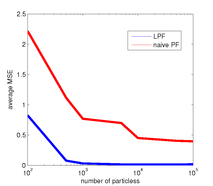
We implement the measure-theoretic extension of BLOG and evaluate our inference algorithms on three models where naive algorithms fail: (1) the GPA model (GPA); (2) the noisy scale model (Scale); and (3) a SSM, the aircraft tracking model (Aircraft-Tracking). The implementation is based on the BLOG’s C++ compiler (Wu et al., 2016).

GPA model: Fig. 1 contains the BLOG code for the GPA example as explained in Sec. 5. Since the GPA of David is exactly 4, the Bayes rule tells that David must be from USA. We evaluate LLW and the naive LW on this model in Fig 4(a), where the naive LW produces a completely wrong answer.

Scale model: In the noisy scale example (Fig. 3), we have an even number of coins and there might be a fake coin among them (Line 4). The fake coin will be slightly heavier than a normal coin (Line 2-3). We divide the coins into two halves and place them onto a noisy scale. When no fake coin, the scale always balances (Line 7). When there is a fake coin, the scale will noisily reflect the weight difference with standard deviation $\sigma$ (sigma in Line 6). Now we observe that the scale is balanced (Line 8) and we would like to infer whether a fake coin exists. We again compare LLW against the naive LW with different choices of the $\sigma$ parameter in Fig. 4(b). Since the scale is precisely balanced, there must not be a fake coin. LLW always produces the correct answer while for the naive LW, the result is incorrect and highly depends on the $\sigma$ parameter: as $\sigma$ increases, the output approaches the true probability.

Aircraft-Tracking model: Fig. 5 shows a simplified BLOG model for the aircraft tracking example. In this state-space model, we have $N=6$ radar points (Line 1) and a single aircraft to track. Both the radars and the aircraft are considered as points on a 2D plane. The prior of the aircraft movement is a Gaussian process (Line 3 to 6). Each radar $r$ has an effective range radius(r): if the aircraft is within the range, the radar will noisily measure the distance from the aircraft to its own location (Line 13); if the aircraft is out of range, the radar will almost surely just output its radius (Line 10 to 11). Now we observe the measurements from all the radar points for $T$ time steps and we want to infer the location of the aircraft. With the measure-theoretic extension, a generalized BLOG program is more expressive for modeling truncated sensors: if a radar outputs exactly its radius, we can surely infer that the aircraft must be out of the effective range of this radar. However, this information cannot be captured by the original BLOG language. To illustrate this case, we manually generate a synthesis dataset of $T=8$ time steps and evaluate LPF against the naive particle filter with different number of particles in Fig. 4(c). We take the mean of the samples from all the particles as the predicted aircraft location. Since we know the ground truth, we measure the average mean square error between the true location and the prediction. LPF accurately predicts the true locations while the naive PF converges to the wrong results.

1  type t_radar; distinct t_radar R[6];
2  // model aircraft movement
3  random Real X(Timestep t) ~ if t == @0
4    then Gaussian(2, 1) else Gaussian(X(prev(t)), 4);
5  random Real Y(Timestep t) ~ if t == @0
6    then Gaussian(-1, 1) else Gaussian(Y(prev(t)), 4);
7  // observation model of radars
8  random Real obs_dist(Timestep t, t_radar r) ~
9    if dist(X(t),Y(t),r) > radius(r) then
10     mixed({radius(r)->0.999,
11    ΨTruncatedGauss(radius(r),0.01,0,radius(r))->0.001})
12   else
13     TruncatedGauss(dist(X(t),Y(t),r),0.01,0,radius(r));
14 // observation and query
15 obs obs_dist(@0, R[0]) = ...;
16 ... // evidence numbers omitted
17 query X(t) for Timestep t;
18 query Y(t) for Timestep t;

Figure 5: BLOG code for the Aircraft-Tracking example

7 Conclusion

In this paper, we proposed the measure-theoretic Bayesian network, a general framework to generalize existing PPL semantics to support random variables over arbitrary measure spaces. We then developed provably correct inference algorithms to handle discrete-continuous mixtures. We also incorporate MTBNs into a widely used PPL, BLOG, by a simple syntax extension and implement the new algorithms into the generalized BLOG language, which makes the system practical for a much larger domain of applications.

We also believe that together with the foundational inference algorithms, our proposed rigorous framework will facilitate the development of powerful techniques for probabilistic reasoning in practical applications from a much wider range of scientific areas.

Acknowledgment

This work is supported by the DARPA PPAML program, contract FA8750-14-C-0011. Simon S. Du is funded by NSF grant IIS1563887, AFRL grant FA8750-17-2-0212 and DARPA D17AP00001.

Appendix A Background on Measure-theoretical Probability Theory

We assume familiarity with measure-theoretic approaches to probability theory, but provide the fundamental definitions. The standard Borel $\sigma$-algebra is assumed in all the discussion. See (Durrett, 2013) and (Kallenberg, 2002) for introduction and further details.

A measurable space $(X,\mathcal{X})$ (space, for short) is an underlying set $X$ paired with a $\sigma$-algebra $\mathcal{X}\subseteq 2^{X}$ of measurable subsets of $X$, i.e., a family of subsets containing the underlying set $X$ which is closed under complements and countable unions. We’ll denote the measurable space simply by $\mathcal{X}$ where no ambiguity results. A function $f\colon\mathcal{X}\to\mathcal{Y}$ between measurable spaces is measurable if measurable sets pullback to measurable sets: $f^{-1}(B)\in\mathcal{X}$ for all $B\in\mathcal{Y}$. A measure $\mu$ on a measurable space $\mathcal{X}$ is a function $\mu\colon\mathcal{X}\to[0,\infty]$ which satisfies countable additivity: for any countable sequence $A_{1},A_{2},\dots\in\mathcal{X}$ of disjoint measurable sets $\mu(\cup_{i}A_{i})=\sum_{i}\mu(A_{i})$. $\mathop{\mathbb{P}}_{\mu}[S]$ denotes the probability of a statement $S$ under the base measure $\mu$, and similarly for conditional probabilities. A probability kernel is the measure-theoretic generalization of a conditional distribution. It is commonly used to construct measures over a product space, analogously to how conditional distributions are used to define joint distributions in the chain rule.

Definition A.1.

A probability kernel $K$ from one measurable space $\mathcal{X}$ to another $\mathcal{Y}$ is a function $K\colon X\times\mathcal{Y}\to[0,1]$ such that (a) for every $x\in X$, $K(x,\cdot)$ is a probability measure over $\mathcal{Y}$, and (b) for every $B\in\mathcal{Y}$, $K(\cdot,B)$ is a measurable function from $\mathcal{X}$ to $[0,1]$.

Given an arbitrary index set $T$ and spaces $\mathcal{X}_{t}$ for each index $t\in T$, the product space $\mathcal{X}=\prod_{t\in T}\mathcal{X}_{t}$ is the space with underlying set $X=\prod_{t\in T}X_{t}$ the Cartesian product of the underlying sets, adorned with the smallest $\sigma$-algebra such that the projection functions $\pi_{t}\colon\mathcal{X}\to\mathcal{X}_{t}$ are measurable.

Appendix B MTBNs Represent Unique Measures

We prove here Theorem 3.6. Its proof requires a series of intermediate results. We first define a projective family of measures. This gives a way to recursively construct our measure $\mu$. We define a notion of consistency such that every consistent projective family constructs a measure that $M$ represents. We end by giving an explicit characterization of the unique consistent projective family, and thus of the unique measure $M$ represents. The appendix contains additional technical material required in the proofs.

Intuitively, the main objective of this section is to show that an MTBN defines a unique measure that “factorizes” according to the network, as an extension to the corresponding result for Bayes Nets.

B.1 Consistent projective family of measures

Let $K$ be a kernel from $\mathcal{X}\to\mathcal{Y}$ and $L$ a kernel from $\mathcal{Y}\to\mathcal{Z}$. Their composition $K\circ L$ (note the ordering!) is a kernel from $\mathcal{X}$ to $\mathcal{Z}$ defined for $x\in X$, $C\in\mathcal{Z}$ by:

$$(K\circ L)(x,C)=\int K(x,dy)\int L(y,dz)\,1_{C}(z).$$ (5)

To allow uniform notation, we will treat measurable functions and measures as special cases of kernels. A measurable function $f\colon X\to Y$ corresponds to the kernel $K_{f}$ from $\mathcal{X}$ to $\mathcal{Y}$ given by $K_{f}(x,B)=1(f(x)\in B)$ for $x\in X$ and $B\in\mathcal{Y}$. A measure $\mu$ on a space $\mathcal{X}$ is a kernel $K_{\mu}$ from $1$, the one element measure space, to $\mathcal{X}$ given by $K_{\mu}(\cdot,A)=\mu(A)$ for $A\in\mathcal{X}$. Where this yields no confusion, we use $f$ and $\mu$ in place of $K_{f}$ and $K_{\mu}$. (5) simplifies if the kernels are measures or functions. Let $\mu$ be a measure on $\mathcal{Y}_{1}$, $K$ be a kernel from $\mathcal{X}_{1}$ to $\mathcal{Y}_{1}$, $f$ be a measurable function from $\mathcal{X}_{2}$ to $\mathcal{X}_{1}$, and $g$ be a measurable function from $\mathcal{Y}_{1}$ to $\mathcal{Y}_{2}$. Then $\mu\circ g$ is a measure on $\mathcal{Y}_{2}$ and $f\circ K\circ g$ is a kernel from $\mathcal{X}_{2}$ to $\mathcal{Y}_{2}$ with: $(\mu\circ g)(B)=\mu(g^{-1}(B))$, and $(f\circ K\circ g)(x,B)=K(f(x),g^{-1}(B))$.

Let $\Lambda$ denote the class of upwardly closed sets: subsets of $V$ containing all their elements’ parents.

Definition B.1.

A projective family of measures is a family $\{\mu_{U}:U\in\Lambda\}$ consisting of a measure $\mu_{U}$ on $\mathcal{X}_{U}$ for every $U\in\Lambda$ such that whenever $W\subseteq U$ we have $\mu_{W}=\mu_{U}\circ\pi^{U}_{W}$, i.e., for all $A\in\mathcal{X}_{W}$, $\mu_{W}(A)=\mu_{U}((\pi^{U}_{W})^{-1}(A))$.

Def. B.1 captures the measure-theoretic version of the probability of a subset of variables being equal to the marginals obtained while “summing out” the probabilities of the other variables in a joint distribution.

Definition B.2.

Let $\mu$ be a measure on a measure space $\mathcal{X}$, and $K$ a kernel from $\mathcal{X}$ to a measure space $\mathcal{Y}$. Then $\mu\otimes K$ is the measure on $\mathcal{X}\times\mathcal{Y}$ defined for $B\in\mathcal{X}\otimes\mathcal{Y}$ by: $(\mu\otimes K)(B)=\int\mu(dx)\int K(x,dy)\,1_{B}(x,y)$.

Def. B.2 defines the operation of composing a conditional probability with a prior on a parent, to obtain the corresponding joint distribution.

Definition B.3.

Let $K_{w}$ for $w\in W$ be kernels from $\mathcal{X}_{U}$ to $\mathcal{X}_{\{w\}}$. Denote by $\prod_{w\in W}K_{w}$ the kernel from $\mathcal{X}_{U}$ to $\mathcal{X}_{W}$ defined for each $x_{U}\in\mathcal{X}_{U}$ by the infinite product of measures: $\left(\prod_{w\in W}K_{w}\right)(x_{U},\cdot)=\otimes_{w\in W}K_{w}(x_{U},\cdot)$.

See (Kallenberg, 2002) 1.27 and 6.18 for definition and existence of infinite products of measures. Def. B.3 captures the kernel representation for taking the equivalent of products of conditional distributions of a set of variables with a common set $U$ of parents.

Definition B.4.

A projective family $\{\mu_{U}:U\in\Lambda\}$ is consistent with $M$ if for any $W,U\in\Lambda$ such that $W\subset U$ and ${\rm pa}(U)\subseteq W$, then: $\mu_{U}=\mu_{W}\otimes\prod_{u\in U\setminus W}(\pi^{W}_{{\rm pa}(u)}\circ K_{u})$.

Consistency in Def. B.4 captures the global condition that we would like to see in a generalization of a Bayes network. Namely, the distribution of any set of parent-closed random variables should “factorize” according to the network

A projective family $\{\mu_{U}:U\in\Lambda\}$ is consistent with $M$ exactly when $M$ represents $\mu_{V}$:

Lemma B.5.

Let $\mu$ be a measure on $\mathcal{X}_{V}$, and define the projective family $\{\mu_{U}:U\in\Lambda\}$ by $\mu_{U}=\mu\circ\pi^{V}_{U}$. This projective family is consistent with $M$ iff $M$ represents $\mu$.

Proof.

First we’ll relate consistency (Def. 8) with conditional expectation and distribution properties of random variables. Take any $W,U\in\Lambda$ such that $W\subset U$ and ${\rm pa}(U)\subseteq W$ and observe that the following are equivalent:

• $\mu_{U}=\mu_{W}\otimes\prod_{u\in U\setminus W}(\pi^{W}_{{\rm pa}(u)}\circ K_{u})$

• $\prod_{u\in U\setminus W}(\pi^{W}_{{\rm pa}(u)}\circ K_{u})$ is a version of the conditional distribution of $X_{U\setminus W}$ given $X_{W}$,

• $K_{u}$ is a version of the conditional distribution of $X_{u}$ given $X_{{\rm pa}(u)}$ for all $u\in U\setminus W$, and $\{X_{W},X_{u}:u\in U\setminus W\}$ are mutually independent conditional on $X_{{\rm pa}(U)}$.

The forward direction is straightforward. For the converse we use the fact that conditional independence of families of random variables holds if it holds for all finite subsets, establishing that by chaining conditional independence (see (Kallenberg, 2002) p109 and 6.8). ∎

Lemma B.5 shows that Def. B.4 follows iff an MTBN represents the joint distribution – in other words, it follows iff the local Markov property holds.

B.2 There exists a unique consistent family

Each vertex $v\in V$ is assigned the unique minimal ordinal $d(v)$ such that $d(u)<d(v)$ whenever $(u,v)\in E$ (see (Jech, 2003) for an introduction to ordinals). For any $U\in\Lambda$ denote by $U^{\alpha}=\{u\in U:v(u)<\alpha\}$ the restriction of $U$ to vertices of depth less than $\alpha$. Defining $D=\sup_{v\in V}(d(v)+1)$, the least strict upper bound on depth, we have that $U^{D}=U$ for all $U\in\Lambda$. In the following, fix a limit ordinal $\lambda$.

Definition B.6.

$\{\nu_{\alpha}:\alpha<\lambda\}$ is a projective sequence of measures on $\mathcal{X}_{U_{\alpha}}$ if whenever $\alpha<\beta<\lambda$ we have $\nu_{\alpha}=\nu_{\beta}\circ\pi^{U_{\beta}}_{U_{\alpha}}$.

Def. B.6 generalizes the notion of subset relationships and the marginalization operations that hold between supersets and subsets to the case of infinite dependency chains

Definition B.7.

The limit $\lim_{\alpha<\lambda}\nu_{\alpha}$ of a projective sequence $\{\nu_{\alpha}:\alpha<\lambda\}$ of measures is the unique measure on $\mathcal{X}_{U}$ such that $\nu_{\alpha}=(\lim_{\alpha<\lambda}\nu_{\alpha})\circ\pi^{U}_{U_{\alpha}}$ for all $\alpha<\beta$.

Definition B.8.

Given any $U\in\Lambda$, inductively define a measure $\mu_{U}^{\alpha}$ on $\mathcal{X}_{U^{\alpha}}$ by

$$\mu_{U}^{0} =1,$$

$$\mu_{U}^{\alpha+1} =\mu^{\alpha}_{U}\otimes\prod_{v\in U:d(v)=\alpha}(\pi^{U^{\alpha}}_{{\rm pa}(v)}\circ K_{v}),$$

$$\mu_{U}^{\lambda} =\lim_{\alpha<\lambda}\mu_{U}^{\alpha}\hskip 18.49988pt\text{if $\lambda$ is a limit ordinal.}$$

$\mu_{U}^{\alpha}$ stabilizes for $\alpha\geq D$ to define a measure on $\mathcal{X}_{U}$.

The above definition is coherent as $\mu_{U}^{\alpha}$ can be inductively shown to be a projective sequence. Lemma B.9 and B.10 allow us to show in Theorem B.11 that $\{\mu_{U}^{D}:U\in\Lambda\}$ is the unique consistent projective family of measures.

Lemma B.9.

If $W\subseteq U$ for $W,U\in\Lambda$, then for all $\alpha$: $\mu_{W}^{\alpha}=\mu_{U}^{\alpha}\circ\pi^{U^{\alpha}}_{W^{\alpha}}.$

Proof is in Appx. C.

Lemma B.10.

If $W\subset U$ where $W,U\in\Lambda$, and if ${\rm pa}(U)\subseteq W$, then $W^{\alpha}\subset U^{\alpha}$, ${\rm pa}(U^{\alpha})\subseteq W^{\alpha}$, and $\mu_{U}^{\alpha}=\mu_{W}^{\alpha}\otimes\prod_{u\in U^{\alpha}\setminus W^{\alpha}}(\pi^{W^{\alpha}}_{{\rm pa}(u)}\circ K_{u}).$

Proof is in Appx. D.

Using the above, the following shows MTBNs satisfy the properties (1-3) mention in the beginning of Sec. 1.1:

Theorem B.11.

$\{\mu_{U}^{D}:U\in\Lambda\}$ is the unique projective family of measures consistent with $M$.

Proof is in Appx. E.

Intuitively, by Lemma B.9 and Lemma B.10, we assert that consistency holds for any ordinal-bounded (prefix in terms of parent ordering) sub-network. Then the main result, Thm. B.11, follows by setting this bound appropriately. Finally Lemma B.5 and Theorem B.11 lead to Theorem 3.6.

Note that combining Thm. 3.6 and Thm. 5.6 lead to all the 4 desired properties mentioned in Sec. 1.1.

Appendix C Proof for Lemma B.9

Proof.

Proof by induction. Trivially true for $\alpha=0$, so suppose this holds for $\alpha$, and consider $\alpha+1$. Then:

$$\mu^{\alpha+1}_{W} =\mu^{\alpha}_{W}\otimes\prod_{v\in W:d(v)=\alpha}(\pi^{W^{\alpha}}_{{\rm pa}(v)}\circ K_{v})$$

$$=\left(\mu_{U}^{\alpha}\circ\pi^{U^{\alpha}}_{W^{\alpha}}\right)$$

$$\hskip 18.49988pt\otimes\left(\left(\prod_{v\in U:d(v)=\alpha}(\pi^{W^{\alpha}}_{{\rm pa}(v)}\circ K_{v})\right)\circ\pi^{U^{\alpha+1}\setminus U^{\alpha}}_{W^{\alpha+1}\setminus W^{\alpha}}\right)$$

$$=\left(\mu_{U}^{\alpha}\otimes\left(\pi^{U^{\alpha}}_{W^{\alpha}}\circ\prod_{v\in U:d(v)=\alpha}(\pi^{W^{\alpha}}_{{\rm pa}(v)}\circ K_{v})\right)\right)$$

$$\hskip 18.49988pt\circ(\pi^{U^{\alpha}}_{W^{\alpha}}\times\pi^{U^{\alpha+1}\setminus U^{\alpha}}_{W^{\alpha+1}\setminus W^{\alpha}})$$

$$=\left(\mu^{\alpha}_{U}\otimes\prod_{v\in U:d(v)=\alpha}(\pi^{U^{\alpha}}_{{\rm pa}(v)}\circ K_{v})\right)\circ\pi^{U^{\alpha+1}}_{W^{\alpha+1}}$$

$$=\mu_{U}^{\alpha+1}\circ\pi^{U^{\alpha+1}}_{W^{\alpha+1}}$$

The first step by Def. 12, the second by inductive hypothesis and Lemma G.11 as $\{v\in W:d(v)=\alpha\}=W^{\alpha+1}\setminus W^{\alpha}$ and $\{v\in U:d(v)=\alpha\}=U^{\alpha+1}\setminus U^{\alpha}$, the third by Lemma G.6, the fourth by Lemma G.10 since $\pi^{U^{\alpha}}_{{\rm pa}(v)}=\pi^{W^{\alpha}}_{{\rm pa}(v)}\circ\pi^{U^{\alpha}}_{W^{\alpha}}$ and by elementary properties of projections, and the fifth by Definition B.8.

Finally, suppose $\lambda$ is a limit ordinal. We need to show:

$$\lim_{\alpha<\lambda}\left(\mu_{U}^{\alpha}\circ\pi^{U^{\alpha}}_{W^{\alpha}}\right)=\left(\lim_{\alpha<\lambda}\mu_{U}^{\alpha}\right)\circ\pi^{U^{\lambda}}_{W^{\lambda}}.$$

This follows from Lemma G.2 because for all $\alpha<\lambda$ we have:

$$\left(\left(\lim_{\alpha<\lambda}\mu_{U}^{\alpha}\right)\circ\pi^{U^{\lambda}}_{W^{\lambda}}\right)\circ\pi^{W^{\lambda}}_{W^{\alpha}} =\left(\left(\lim_{\alpha<\lambda}\mu_{U}^{\alpha}\right)\circ\pi^{U^{\lambda}}_{U^{\alpha}}\right)\circ\pi^{U^{\alpha}}_{W^{\alpha}}$$

$$=\mu^{\alpha}_{U}\circ\pi^{U^{\alpha}}_{W^{\alpha}}$$

The first by properties of projections, the second by Lemma G.2 characterizing limits. ∎

Appendix D Proof for Lemma B.10

Proof.

Trivial for $\alpha=0$, so suppose this holds for $\alpha$, and consider $\alpha+1$. Then:

$$\mu_{U}^{\alpha+1}$$

$$=\mu^{\alpha}_{U}\otimes\prod_{v\in U:d(v)=\alpha}(\pi^{U^{\alpha}}_{{\rm pa}(v)}\circ K_{v})$$

$$=\mu_{W}^{\alpha}\otimes\prod_{u\in U^{\alpha}\setminus W^{\alpha}}(\pi^{W^{\alpha}}_{{\rm pa}(u)}\circ K_{u})\otimes\prod_{v\in U:d(v)=\alpha}(\pi^{U^{\alpha}}_{{\rm pa}(v)}\circ K_{v})$$

$$=\mu_{W}^{\alpha}\otimes\prod_{u\in U^{\alpha+1}\setminus W^{\alpha}}(\pi^{W^{\alpha}}_{{\rm pa}(u)}\circ K_{u})$$

$$=\mu^{\alpha}_{W}\otimes\prod_{v\in W:d(v)=\alpha}(\pi^{W^{\alpha}}_{{\rm pa}(v)}\circ K_{v})$$

$$\hskip 18.49988pt\hskip 18.49988pt\hskip 18.49988pt\hskip 18.49988pt\hskip 18.49988pt\otimes\prod_{u\in U^{\alpha+1}\setminus W^{\alpha+1}}(\pi^{W^{\alpha+1}}_{{\rm pa}(u)}\circ K_{u})$$

$$=\mu^{\alpha+1}_{W}\otimes\prod_{u\in U^{\alpha+1}\setminus W^{\alpha+1}}(\pi^{W^{\alpha+1}}_{{\rm pa}(u)}\circ K_{u}),$$

The first step by Definition B.8, the second by inductive hypothesis. The third by Lemmas G.8 and G.9 since $U^{\alpha+1}\setminus W^{\alpha}=U^{\alpha}\setminus W^{\alpha}\cup\{v\in U:d(v)=\alpha\}$ where the union is disjoint, and as ${\rm pa}(v)\subseteq W^{\alpha}$ when $v\in U$ and $d(v)=\alpha$ implies that $\pi^{U^{\alpha}}_{{\rm pa}(v)}=\pi^{U^{\alpha}}_{W^{\alpha}}\circ\pi^{W^{\alpha}}_{{\rm pa}(v)}$. The fourth by Lemmas G.8 and G.9 since $U^{\alpha+1}\setminus W^{\alpha}=U^{\alpha+1}\setminus W^{\alpha+1}\cup\{v\in W:d(v)=\alpha\}$ where the union is disjoint, and as ${\rm pa}(u)\subseteq W^{\alpha}$ when $u\in U^{\alpha+1}\setminus W^{\alpha+1}$ implies that $\pi^{W^{\alpha+1}}_{{\rm pa}(v)}=\pi^{W^{\alpha+1}}_{W^{\alpha}}\circ\pi^{W^{\alpha}}_{{\rm pa}(v)}$. Finally, the fifth by Definition B.8.

Finally, suppose $\lambda$ is a limit ordinal. The result will follow from the inductive hypothesis, Definition B.8, and as limits preserve products Lemma G.7 if we can show that

$$\lim_{\alpha<\lambda}\prod_{u\in U^{\alpha}\setminus W^{\alpha}}(\pi^{W^{\alpha}}_{{\rm pa}(u)}\circ K_{u})=\prod_{u\in U^{\lambda}\setminus W^{\lambda}}(\pi^{W^{\lambda}}_{{\rm pa}(u)}\circ K_{u}).$$

First we must show the limit on the left is well-defined. Note that the kernel inside the limit maps from $\mathcal{X}_{W^{\alpha}}$ to $\mathcal{X}_{U^{\alpha}\setminus W^{\alpha}}$. As $W^{\alpha}$ and $U^{\alpha}\setminus W^{\alpha}$ are both increasing sets, we verify projective sequence property by taking any $\beta>\alpha$ and observing that

$$\pi^{W^{\beta}}_{W^{\alpha}}\circ\prod_{u\in U^{\alpha}\setminus W^{\alpha}}(\pi^{W^{\alpha}}_{{\rm pa}(u)}\circ K_{u})$$

$$=\prod_{u\in U^{\alpha}\setminus W^{\alpha}}(\pi^{W^{\beta}}_{{\rm pa}(u)}\circ K_{u})$$

$$=\left(\prod_{u\in U^{\beta}\setminus W^{\beta}}(\pi^{W^{\beta}}_{{\rm pa}(u)}\circ K_{u})\right)\circ\pi^{U^{\beta}\setminus W^{\beta}}_{U^{\alpha}\setminus W^{\alpha}}$$

the first step from Lemma G.10 and properties of projections, and the second from Lemma G.11.

Finally, we must show the expression on the right satisfies the properties characterizing the limit. However, observe this follows from our demonstration of the projective sequence property above by simply replacing $\beta$ with $\lambda$. ∎

Appendix E Proof for Theorem B.11

Proof.

That this is a consistent projective family follows from Lemmas B.9 and B.10 since $U^{D}=U$ for all $U\in\Lambda$.

For uniqueness, let $\{\hat{\mu}_{U}:U\in\Lambda\}$ be a consistent projective family of measures, any fix any $U\in\Lambda$. We’ll show inductively that $\hat{\mu}_{U^{\alpha}}=\mu_{U}^{\alpha}$, and thus with $\alpha=D$ that $\hat{\mu}_{U}=\mu_{U}$, giving our result. This is trivial for $\alpha=0$, so inductively suppose it holds for $\alpha$. But then:

$$\hat{\mu}_{U^{\alpha+1}} =\hat{\mu}_{U^{\alpha}}\otimes\prod_{u\in U^{\alpha+1}\setminus U^{\alpha}}(\pi^{U^{\alpha}}_{{\rm pa}(u)}\circ K_{u})$$

$$=\mu_{U}^{\alpha}\otimes\prod_{u\in U^{\alpha+1}\setminus U^{\alpha}}(\pi^{U^{\alpha}}_{{\rm pa}(u)}\circ K_{u}).$$

The first step by consistency of $\{\hat{\mu}_{U}\}$ (Definition B.4) since $U^{\alpha}\subseteq U^{\alpha+1}$ and ${\rm pa}(U^{\alpha+1})\subseteq U^{\alpha}$, the second by inductive hypothesis, and the third by Definition B.8.

Let $\alpha$ be a limit ordinal. Since $\{\hat{\mu}_{U^{\alpha}}\}$ is a projective family and $U^{\alpha}=\bigcup_{\beta<\alpha}U^{\beta}$, by Lemma G.2 $\hat{\mu}_{U^{\alpha}}=\lim_{\beta<\alpha}\hat{\mu}_{U^{\beta}}$. By definition $\mu_{U}^{\alpha}=\lim_{\beta<\alpha}\mu_{U}^{\beta}$. Then since $\mu_{U}^{\beta}=\hat{\mu}_{U^{\beta}}$ for $\beta<\alpha$ inductively, $\mu_{U}^{\alpha}=\hat{\mu}_{U^{\alpha}}$ as the limit of this sequence is unique. ∎

Appendix F Proof of Lemma 5.4

Proof.

The possible world $\langle U^{\sigma},I^{\sigma}\rangle$ is defined as follows. $U^{\sigma}=\langle U^{\sigma}_{1},\ldots,U^{\sigma}_{k}\rangle$, where $U_{j}^{\sigma}=\{c_{j}:c_{j}$ is a distinct constant of type $\tau_{j}$ in $\mathcal{M}\}$ $\cup$ $\{u_{\nu,\bar{u},l}\in\mathcal{U}_{\mathcal{M}}:\nu$ is a number statement of type $\tau_{j}$ and $\sigma(V_{\nu}[\bar{u}])\geq l\}$.

$I^{\sigma}$ is defined as follows. For each function symbol $f(\bar{x})$ in $\mathcal{M}$, for each tuple $\bar{u}$ of the type of $\bar{x}$ constructed using elements of $U^{\sigma}$, $[f]^{\sigma}(\bar{u})=\sigma(V_{f}[\bar{u}])$. The element $\sigma(V_{f}[\bar{u}])$ is a member of $U^{\sigma}$ because of the last clause in the definition of consistent assignments (Def. 5.3) and the construction of $U^{\sigma}$. ∎

Appendix G Additional Technical Details

For reasons of space, we present the following without their (straightforward) proofs.

Lemma G.1.

If $\mu$ is a measure on $\mathcal{X}$, and is $K$ a kernel from $\mathcal{X}$ to $\mathcal{Y}$, then $(\mu\otimes K)\circ\pi^{\mathcal{X}\times\mathcal{Y}}_{\mathcal{X}}=\mu.$

Lemma G.2.

A projective sequence of measures has a unique limit.

Fix an ordinal $\lambda$, and suppose $\{U_{\alpha}\subseteq V:\alpha<\lambda\}$ is an increasing sequence of subsets of $V$, i.e., such that if $\alpha<\beta<\lambda$ then $U_{\alpha}\subseteq U_{\beta}$. Define $U=\bigcup_{\alpha<\lambda}U_{\alpha}$. Let $\{W_{\alpha}\subseteq V:\alpha<\lambda\}$ and $W$ be another such sequence, supposing $U$ and $W$ are disjoint.

Definition G.3.

$\{K_{\alpha}:\alpha<\lambda\}$ is a projective sequence of kernels from $\mathcal{X}_{U_{\alpha}}$ to $\mathcal{X}_{W_{\alpha}}$ if whenever $\alpha<\beta<\lambda$ we have $\pi^{U_{\beta}}_{U_{\alpha}}\circ K_{\alpha}=K_{\beta}\circ\pi^{W_{\beta}}_{W_{\alpha}}.$

Definition G.4.

The limit $\lim_{\alpha<\beta}K_{\alpha}$ of a projective sequence $\{K_{\alpha}:\alpha<\lambda\}$ of kernels is the unique kernel from $\mathcal{X}_{U}$ to $\mathcal{X}_{W}$ such that for all $\alpha<\lambda$ $\pi^{U}_{U_{\alpha}}\circ K_{\alpha}=\left(\lim_{\alpha<\beta}K_{\alpha}\right)\circ\pi^{W}_{W_{\alpha}}.$

Lemma G.5.

A projective sequence of kernels has a unique limit.

Lemma G.6.

Let $\mathcal{X}_{1},\mathcal{Y}_{1},\mathcal{X}_{2},\mathcal{Y}_{2}$ be measurable spaces, $\mu$ be a measure on $\mathcal{X}_{1}$, $K$ a kernel from $\mathcal{X}_{2}$ to $\mathcal{Y}_{1}$, $f\colon\mathcal{X}_{1}\to\mathcal{X}_{2}$ a measurable function, and $g\colon\mathcal{Y}_{1}\to\mathcal{Y}_{2}$ a measurable function. Then: $(\mu\otimes(f\circ K))\circ(f\times g)=(\mu\circ f)\otimes(K\circ g)$ where $f\times g$ is the measurable function mapping $(x,y)$ to $((f(x),g(y))$.

Lemma G.7.

Let $\nu_{\alpha}$ and $K_{\alpha}$ be as in Lemmas G.2 and G.5. Then $\lim_{\alpha<\lambda}(\nu_{\alpha}\otimes K_{\alpha})=(\lim_{\alpha<\lambda}\nu_{\alpha})\otimes(\lim_{\alpha<\lambda}K_{\alpha}).$

Lemma G.8.

$\mu$ measure on $\mathcal{X}$, $K_{1}$ a kernel from $\mathcal{X}$ to $\mathcal{Y}_{1}$, $K_{2}$ a kernel from $\mathcal{X}$ to $\mathcal{Y}_{2}$, $\mu\otimes K_{1}\otimes(\pi^{\mathcal{X}\times\mathcal{Y}_{1}}_{\mathcal{X}}\circ K_{2})=\mu\otimes\prod_{i=1,2}K_{i}$. where by abuse of notation $\pi^{\mathcal{X}\times\mathcal{Y}_{1}}_{\mathcal{X}}$ denotes the projection from $\mathcal{X}\times\mathcal{Y}_{1}$ to $\mathcal{X}$.

Lemma G.9.

If $K_{i,j}$ are kernels from $\mathcal{X}$ to $\mathcal{Y}_{i,j}$ then $\prod_{i}\prod_{j}K_{i,j}=\prod_{i,j}K_{i,j}$.

Lemma G.10.

If $f\colon\mathcal{X}^{\prime}\to\mathcal{X}$ and $K_{i}$ are kernels from $\mathcal{X}$ to $\mathcal{Y}_{i}$ then $f\circ\prod_{i}K_{i}=\prod_{i}f\circ K_{i}$.

Lemma G.11.

If $K_{v}$ for $v\in U$ are kernels from $\mathcal{X}$ to $\mathcal{X}_{v}$, and $W\subseteq U$ then $\left(\prod_{v\in U}K_{v}\right)\circ\pi^{U}_{W}=\prod_{v\in W}K_{v}$.

Lemma G.12.

Let $(X,\mathcal{X})$ be a measurable space, $X,X_{1},X_{2},\dots$ an iid random sequence on $\mathcal{X}$, and $w(x)$ be non-negative real-valued function of $(X,\mathcal{X})$. Then $\frac{\sum_{i=1}^{n}w(X_{i})f(X_{i})}{\sum_{i=1}^{n}w(X_{i})}\stackrel{{\scriptstyle\rm a.s.}}{{\to}}\frac{\mathop{\mathbb{E}}w(X)f(X)}{\mathop{\mathbb{E}}w(X)}$.

Lemma G.13.

For any measurable set $E$ and measurable function $f(x)$: $\frac{\mathop{\mathbb{E}}P(E|X)f(X)}{\mathop{\mathbb{E}}P(E|X)}=\mathop{\mathbb{E}}[f(X)|E].$

References

- Arora et al. (2013) Arora, N. S., Russell, S., and Sudderth, E. NET-VISA: Network processing vertically integrated seismic analysis. Bulletin of the Seismological Society of America, 103(2A):709–729, 2013.
- Carpenter et al. (2016) Carpenter, B., Gelman, A., Hoffman, M., Lee, D., Goodrich, B., Betancourt, M., Brubaker, M. A., Guo, J., Li, P., Riddell, A., et al. Stan: A probabilistic programming language. Journal of Statistical Software, 20(2):1–37, 2016.
- Choi et al. (2010) Choi, J., Amir, E., and Hill, D. J. Lifted inference for relational continuous models. In UAI, volume 10, pp. 126–134, 2010.
- Doucet et al. (2001) Doucet, A., De Freitas, N., and Gordon, N. An introduction to sequential Monte Carlo methods. In Sequential Monte Carlo methods in practice, pp. 3–14. Springer, 2001.
- Durrett (2013) Durrett, R. Probability: Theory and Examples. Cambridge University Press, 2013.
- Gao et al. (2017) Gao, W., Kannan, S., Oh, S., and Viswanath, P. Estimating mutual information for discrete-continuous mixtures. In Advances in Neural Information Processing Systems, pp. 5988–5999, 2017.
- Goodman (2013) Goodman, N. D. The principles and practice of probabilistic programming. In ACM SIGPLAN Notices, volume 48, pp. 399–402. ACM, 2013.
- Goodman & Stuhlmüller (2014) Goodman, N. D. and Stuhlmüller, A. The Design and Implementation of Probabilistic Programming Languages. http://dippl.org, 2014. Accessed: 2018-6-5.
- Goodman et al. (2008) Goodman, N. D., Mansinghka, V. K., Roy, D. M., Bonawitz, K., and Tenenbaum, J. B. Church: A language for generative models. In UAI-08, 2008.
- Gutmann et al. (2011a) Gutmann, B., Jaeger, M., and De Raedt, L. Extending problog with continuous distributions. In Inductive Logic Programming, pp. 76–91. Springer, 2011a.
- Gutmann et al. (2011b) Gutmann, B., Thon, I., Kimmig, A., Bruynooghe, M., and De Raedt, L. The magic of logical inference in probabilistic programming. Theory and Practice of Logic Programming, 11(4-5):663–680, 2011b.
- Jech (2003) Jech, T. Set theory. Springer, 2003.
- Kallenberg (2002) Kallenberg, O. Foundations of Modern Probability. Springer, 2002. URL http://www.amazon.com/exec/obidos/redirect?tag=citeulike07-20&path=ASIN/0387953132.
- Kersting & De Raedt (2007) Kersting, K. and De Raedt, L. Bayesian logic programming: Theory and tool. Statistical Relational Learning, pp. 291, 2007.
- Kharchenko et al. (2014) Kharchenko, P. V., Silberstein, L., and Scadden, D. T. Bayesian approach to single-cell differential expression analysis. Nature methods, 11(7):740, 2014.
- Koller et al. (1997) Koller, D., McAllester, D., and Pfeffer, A. Effective Bayesian inference for stochastic programs. In AAAI-97, 1997.
- Kulkarni et al. (2015) Kulkarni, T. D., Kohli, P., Tenenbaum, J. B., and Mansinghka, V. Picture: A probabilistic programming language for scene perception. In Proceedings of the ieee conference on computer vision and pattern recognition, pp. 4390–4399, 2015.
- Lake et al. (2015) Lake, B. M., Salakhutdinov, R., and Tenenbaum, J. B. Human-level concept learning through probabilistic program induction. Science, 350(6266):1332–1338, 2015.
- Le et al. (2017) Le, T. A., Baydin, A. G., and Wood, F. Inference compilation and universal probabilistic programming. In Artificial Intelligence and Statistics, pp. 1338–1348, 2017.
- Li & Russell (2013) Li, L. and Russell, S. J. The BLOG language reference. Technical report, Technical Report UCB/EECS-2013-51, EECS Department, University of California, Berkeley, 2013.
- Mansinghka et al. (2014) Mansinghka, V., Selsam, D., and Perov, Y. Venture: a higher-order probabilistic programming platform with programmable inference. arXiv preprint arXiv:1404.0099, 2014.
- McAllester et al. (2008) McAllester, D., Milch, B., and Goodman, N. D. Random-world semantics and syntactic independence for expressive languages. Technical report, 2008.
- Milch et al. (2005a) Milch, B., Marthi, B., Russell, S. J., Sontag, D., Ong, D. L., and Kolobov, A. BLOG: Probabilistic models with unknown objects. In Proc. of IJCAI, pp. 1352–1359, 2005a.
- Milch et al. (2005b) Milch, B., Marthi, B., Sontag, D., Russell, S., Ong, D. L., and Kolobov, A. Approximate inference for infinite contingent Bayesian networks. In Tenth International Workshop on Artificial Intelligence and Statistics, Barbados, 2005b. URL http://www.gatsby.ucl.ac.uk/aistats/AIabst.htm.
- Milch (2006) Milch, B. C. Probabilistic models with unknown objects. PhD thesis, University of California at Berkeley, Berkeley, CA, USA, 2006.
- Nitti et al. (2016) Nitti, D., De Laet, T., and De Raedt, L. Probabilistic logic programming for hybrid relational domains. Machine Learning, 103(3):407–449, 2016.
- Pearl (1988) Pearl, J. Probabilistic reasoning in intelligent systems: networks of plausible inference. Morgan Kaufmann, 1988.
- Pfeffer (2009) Pfeffer, A. Figaro: An object-oriented probabilistic programming language. Charles River Analytics Technical Report, 137:96, 2009.
- Pierson & Yau (2015) Pierson, E. and Yau, C. Zifa: Dimensionality reduction for zero-inflated single-cell gene expression analysis. Genome biology, 16(1):241, 2015.
- Ramsey (2016) Ramsey, N. All you need is the monad.. what monad was that again. In PPS Workshop, 2016.
- Ritchie et al. (2015) Ritchie, D., Lin, S., Goodman, N. D., and Hanrahan, P. Generating design suggestions under tight constraints with gradient-based probabilistic programming. In Computer Graphics Forum, volume 34, pp. 515–526. Wiley Online Library, 2015.
- Shan & Ramsey (2017) Shan, C.-c. and Ramsey, N. Exact Bayesian inference by symbolic disintegration. In Proceedings of the 44th ACM SIGPLAN Symposium on Principles of Programming Languages, pp. 130–144. ACM, 2017.
- Singla & Domingos (2007) Singla, P. and Domingos, P. Markov logic in infinite domains. In In Proc. UAI-07, 2007.
- Staton (2017) Staton, S. Commutative semantics for probabilistic programming. In European Symposium on Programming, pp. 855–879. Springer, 2017.
- Stuhlmüller & Goodman (2014) Stuhlmüller, A. and Goodman, N. D. Reasoning about reasoning by nested conditioning: Modeling theory of mind with probabilistic programs. Cognitive Systems Research, 28:80–99, 2014.
- Tolpin et al. (2016) Tolpin, D., van de Meent, J. W., Yang, H., and Wood, F. Design and implementation of probabilistic programming language anglican. arXiv preprint arXiv:1608.05263, 2016. URL https://github.com/probprog/anglican-examples/blob/master/worksheets/indian-gpa.clj.
- Tran et al. (2016) Tran, D., Kucukelbir, A., Dieng, A. B., Rudolph, M., Liang, D., and Blei, D. M. Edward: A library for probabilistic modeling, inference, and criticism. arXiv preprint arXiv:1610.09787, 2016.
- Wang & Domingos (2008) Wang, J. and Domingos, P. Hybrid Markov logic networks. In AAAI, volume 8, pp. 1106–1111, 2008.
- Wood et al. (2014a) Wood, F., Meent, J. W., and Mansinghka, V. A new approach to probabilistic programming inference. In Artificial Intelligence and Statistics, pp. 1024–1032, 2014a.
- Wood et al. (2014b) Wood, F., van de Meent, J. W., and Mansinghka, V. A new approach to probabilistic programming inference. In Proceedings of the 17th International conference on Artificial Intelligence and Statistics, pp. 1024–1032, 2014b.
- Wu et al. (2014) Wu, Y., Li, L., and Russell, S. BFiT: From possible-world semantics to random-evaluation semantics in open universe. 3rd NIPS Workshop on Probabilistic Programming, 2014.
- Wu et al. (2016) Wu, Y., Li, L., Russell, S., and Bodik, R. Swift: Compiled inference for probabilistic programming languages. In Proceedings of the 25th International Joint Conference on Artificial Intelligence (IJCAI), 2016.