Realtime Active Sound Source Localization for Unmanned Ground Robots Using a Self-Rotational Bi-Microphone Array

This work presents a novel technique that performs both orientation and distance localization of a sound source in a three-dimensional (3D) space using only the interaural time difference (ITD) cue, generated by a newly-developed self-rotational bi-microphone robotic platform. The system dynamics is established in the spherical coordinate frame using a state-space model. The observability analysis of the state-space model shows that the system is unobservable when the sound source is placed with elevation angles of $90$ and $0$ degree. The proposed method utilizes the difference between the azimuth estimates resulting from respectively the 3D and the two-dimensional models to check the zero-degree-elevation condition and further estimates the elevation angle using a polynomial curve fitting approach. Also, the proposed method is capable of detecting a $90$-degree elevation by extracting the zero-ITD signal ’buried’ in noise. Additionally, a distance localization is performed by first rotating the microphone array to face toward the sound source and then shifting the microphone perpendicular to the source-robot vector by a predefined distance of a fixed number of steps. The integrated rotational and translational motions of the microphone array provide a complete orientation and distance localization using only the ITD cue. A novel robotic platform using a self-rotational bi-microphone array was also developed for unmanned ground robots performing sound source localization. The proposed technique was first tested in simulation and was then verified on the newly-developed robotic platform. Experimental data collected by the microphones installed on a KEMAR dummy head were also used to test the proposed technique. All results show the effectiveness of the proposed technique.

1 INTRODUCTION

The localization problem in the robotic field has been recognized as the most fundamental problem to make robots truly autonomous Borenstein1996. Localization techniques are of great importance for autonomous unmanned systems to identify their own locations (i.e., self-localization) and situational awareness (e.g., locations of surrounding objects), especially in an unknown environment. Mainstream technology for localization is based on computer vision, supported by visual sensors (e.g., cameras), which, however, are subject to lighting and line-of-sight conditions and rely on computationally demanding image-processing algorithms. An acoustic sensor (e.g., a microphone), as a complementary component in a robotic sensing system, does not require a line of sight and is able to work under varying light (or completely dark) conditions in an omnidirectional manner. Thanks to the advancement of microelectromechanical technology, microphones become inexpensive and do not require significant power to operate.

Sound-source localization (SSL) techniques have been developed that identify the location of sound sources (e.g., speech and music) in terms of directions and distances. SSL techniques have been widely used in civilian applications, such as intelligent video conferencing huang2000passive; wang1997voice, environmental monitoring tiete2014soundcompass, human-robot interaction (HRI) for humanoid robotics hornstein2006sound, and robot motion planning NguyenColasVincentEtAl2017, as well as military applications, such as passive sonar for submarine detections, surveillance systems that locate hostile tanks, artillery, incoming missiles kaushik2005review, aircraft blumrich2000medium, and UAVs brandes2007sound. SSL techniques have great potential by itself to enhance the sensing capability of autonomous unmanned systems as well as working together with vision-based localization techniques.

SSL has been achieved by using microphone arrays with more than two microphones TamaiSasakiKagamiEtAl2005; TamaiKagamiAmemiyaEtAl2004; SturimBrandsteinSilverman1997; ValinMichaudRouatEtAl2016; omologo1996acoustic. The accuracy of the localization techniques based on microphone arrays is dictated by their physical sizes brandstein2013microphone; benesty2008microphone; Zietlow2017. Microphone arrays are usually designed using particular (e.g., linear or circular) structures, which result in their relatively large sizes and sophisticated control components for operation. Therefore, it becomes difficult to use them on small robots nor large systems due to the complexity of mounting and maneuvering.

In the past decade, research has been carried out for robots to have auditory behaviors (e.g. getting attention to an event, locating a sound source in potentially dangerous situations, and locating and paying attention to a speaker) by mimicking human auditory systems. Humans perform sound localization with their two ears using integrated three types of cues, i.e., the interaural level difference (ILD), the interaural time difference (ITD), and the spectral information goldstein2016sensation; middlebrooks1991sound. ILD and ITD cues are usually used respectively to identify the horizontal location (i.e., azimuth angle) of a sound source with higher and lower frequencies. Spectral cues are usually used to identify the vertical location (i.e., elevation angle) of a sound source with higher frequencies. Additionally, acoustic landmarks aid towards bettering the SSL by humansZhong2015.

To mimic human acoustic systems, researchers have developed sound source localization techniques using only two microphones. All three types of cues have been used by Rodemann et al. RodemannInceJoublinEtAl2008 in a binaural approach of estimating the azimuth angle of a sound source, while the authors also stated that reliable elevation estimation would need a third microphone. Spectral cues were used by the head-related-transfer-function (HRTF) that was applied to identify both the azimuth and elevation angles of a sound source for binaural sensor platforms Keyrouz2014; gill2000auditory; hornstein2006sound; KeyrouzDiepold2006. The ITD cues have also been used in binaural sound source localization chen2006time, where the problem of cone of confusion Wallach1939 has been overcome by incorporating head movements, which also enable both azimuth and elevation estimation Wallach1939; perrett1997effect. Lu et al. lu2011motion used a particle filter for binaural tracking of a mobile sound source on the basis of ITD and motion parallax but the localization was limited in a two-dimensional (2D) plane and was not impressive under static conditions. Pang et al. PangLiuZhangEtAl2017 presented an approach for binaural azimuth estimation based on reverberation weighting and generalized parametric mapping. Lu et al. lu2007active presented a binaural distance localization approach using the motion-induced rate of intensity change which requires the use of parallax motion and errors up to 3.4 m were observed. Kneip and Baumann LaurentKneip2008 established formulae for binaural identification of the azimuth and elevation angles as well as the distance information of a sound source combining the rotational and translational motion of the interaural axis. However, large localization errors were observed and no solution was given to handle sensor noise nor model uncertainty. Rodemann Rodemann2010 proposed a binaural azimuth and distance localization technique using signal amplitude along with ITD and ILD cues in an indoor environment with a sound source ranging from $0.5\;\text{m}$ to $6\;\text{m}$. However, the azimuth estimation degrades with the distance and reduced error with the required calibration was still large. Kumon and Uozumi kumon2011binaural proposed a binaural system on a robot to localize a mobile sound source but it requires the robot to move with a constant velocity to achieve 2D localization. Also, further study was proposed for a parameter $\alpha_{0}$ introduced in the EKF. Zhong et al. Sun2015; zhong2016active and Gala et al. Gala2018 utilized the extended Kalman filtering (EKF) technique to perform orientation localization using the ITD data acquired by a set of binaural self-rotating microphones. Moreover, large errors were observed in zhong2016active when the elevation angle of a sound source was close to zero.

To the best of our knowledge, the works presented in the literature for SSL using two microphones based on ITD cues mainly provided formulae that calculate the azimuth and elevation angles of a sound source without incorporating sensor noise LaurentKneip2008. The works that use probabilistic recursive filtering techniques (e.g., EKF) for orientation estimation zhong2016active did not conduct any observability analysis on the system dynamics. In other words, no discussion on the limitation of the techniques for orientation estimation was found. In addition, no probabilistic recursive filtering technique was used to acquire distance information of a sound source. This paper aims to address these research gaps.

The contributions of this paper include (1) an observability analysis of the system dynamics for three-dimensional (3D) SSL using two microphones and the ITD cue only; (2) a novel algorithm that provides the estimation of the elevation angle of a sound source when the states are unobservable; and (3) a new EKF-based technique that estimates the robot-sound distance. Both simulations and experiments were conducted to validate the proposed techniques.

The rest of this paper is organized as follows. Section 2 describes the preliminaries. In Section 3, 2D and 3D orientation localization models are presented along with their observability analysis. In Section 4, a novel method is proposed to detect non-observability conditions and a solution to the non-observability problem is presented. Section 5 presents a distance localization model with its observability analysis. The EKF algorithm is presented in Section 6. In Sections 7 and 8, the simulation and experimental results are presented respectively, followed by Section 9, which concludes the paper.

2 PRELIMINARIES

2.1 Calculation of ITD

The only cue used for localization in this paper is the ITD, which is the time difference of a sound signal traveling to the two microphones and can be calculated using the cross-correlation technique Knapp1976The; azaria1984time.

Figure 1: Interaural Time Delay (ITD) estimation between signals $y_{1}(t)$ and $y_{2}(t)$ using the cross-correlation technique.

Consider a single stationary sound source placed in an environment. Let $y_{1}(t)$ and $y_{2}(t)$ be the sound signals captured by two spatially separated microphones in the presence of noise, which are given by Knapp1976The

$$y_{1}(t) =s(t)+n_{1}(t),$$ (1)

$$y_{2}(t) =\delta\cdot s\left(t+t_{d}\right)+n_{2}(t),$$ (2)

where $s\left(t\right)$ is the sound signal, $n_{1}(t)$ and $n_{2}(t)$ are real and jointly stationary random processes, $t_{d}$ denotes the time difference of $s\left(t\right)$ arriving at the two microphones, and $\delta$ is the signal attenuation factor due to different traveling distances of the sound signal to the two microphones. It is commonly assumed that $\delta$ changes slowly and $s(t)$ is uncorrelated with noises $n_{1}(t)$ and $n_{2}(t)$ Knapp1976The. The cross-correlation function of $y_{1}(t)$ and $y_{2}(t)$ is given by

$$R_{y_{1},y_{2}}(\tau)=E\left[y_{1}(t)\cdot y_{2}(t-\tau)\right],$$

where $E\left[\cdot\right]$ represents the expectation operator. Figure 1 shows the process of delay estimation between $y_{1}(t)$ and $y_{2}(t)$, where $H_{1}(f)$ and $H_{2}(f)$ represent scaling functions or pre-filters Knapp1976The. Various techniques can be used to eliminate or reduce the effect of background noise and reverberations Boll1979; BollPulsipher1980; naylor2010speech; spriet2007speech; Gala2010; Gala2011. An improved version of the cross-correlation method incorporating $H_{1}(f)$ and $H_{2}(f)$ is called Generalized Cross-Correlation (GCC) Knapp1976The, which further improves the estimation of time delay.

The time difference of $y_{1}(t)$ and $y_{2}(t)$, i.e., the ITD, is given by $\hat{T}\triangleq\arg\max_{\tau}R_{y_{1},y_{2}}.$ The distance difference of the sound signal traveling to the two microphones is given by $d\triangleq\hat{T}\cdot c_{0},$ where $c_{0}$ is the sound speed and is usually selected to be 345 m/s.

2.2 Far-Field Assumption

The area around a sound source can be divided into five different fields: free field, near field, far field, direct field and reverberant field ISO12001; Hansen2001. The region close to a source where the sound pressure and the acoustic particle velocity are not in phase is regarded as the near field. The range of the near field is limited to a distance from the source equal to approximately a wavelength of sound or equal to three times the largest dimension of the sound source, whichever is the larger. The far field of a source begins where the near field ends and extends to infinity. Under the far-field assumption, the acoustic wavefront reaching the microphones is planar and not spherical, in the sense that the waves travel in parallel i.e. the angle of incidence is the same for the two microphones Calmes2009.

2.3 Observability Analysis

Consider a nonlinear system described by a state-space model

$$\dot{\mathbf{x}} =f\left(\mathbf{x}\right),$$ (3)

$$\mathbf{y} =h\left(\mathbf{x}\right),$$ (4)

where $\mathbf{x}\in\mathbb{R}^{n}$ and $\mathbf{y}\in\mathbb{R}^{m}$ are the state and output vectors, respectively, and $f\left(\cdot\right)$ and $h\left(\cdot\right)$ are the process and output functions, respectively. The observability matrix of the system described by (3) and (4) is then given by hedrick2005control

$$\Omega =\left[\begin{array}[]{ccc}\left(\frac{\partial L_{f}^{0}h}{\partial\mathbf{x}}\right)^{T}&\left(\frac{\partial L_{f}^{1}h}{\partial\mathbf{x}}\right)^{T}&\cdots\end{array}\right]^{T},$$

where the Lie derivatives are given by $L_{f}^{0}h=h\left(\mathbf{x}\right)$ and $L_{f}^{n}h=\frac{\partial L_{f}^{n-1}h}{\partial\mathbf{x}}f$. The system is observable if the observability matrix $\Omega$ has rank $n$.

3 Mathematical Models and Observability Analysis for Orientation Localization

The complete localization of a sound source is usually achieved in two stages, the orientation (i.e., azimuth and elevation angles) localization and distance localization. In this section, the methodology of the orientation localization is presented.

Figure 2: Top view of the robot illustrating different angle definitions due to the rotation of the microphone array.

Figure 3: 3D view of the system for orientation localization.

3.1 Definitions

As shown in Figures 2 and 3, the acoustic signal generated by the sound source $S$ is collected by the left and right microphones, $L$ and $R$, respectively. Let $O$ be the center of the robot as well as the two microphones. The location of $S$ is represented by ($D,\theta,\varphi$), where $D$ is the distance between the source and the center of the robot, i.e., the length of segment $\overline{OS}$, $\theta\in\left[0,\frac{\pi}{2}\right]$ is the elevation angle defined as the angle between $\overline{OS}$ and the horizontal plane, and $\varphi\in\left(-\pi,\pi\right]$ is the azimuth angle defined as the angle measured clockwise from the robot heading vector, $\mathbf{p}$, to $\overline{OS}$. Letting unit vector $\mathbf{q}$ be the orientation (heading) of the microphone array, $\beta$ be the angle between $\mathbf{p}$ and $\mathbf{q}$, and $\psi$ be the angle between $\mathbf{q}$ and $\overline{OS}$, both following a right hand rotation rule, we have

$$\varphi=\psi+\beta.$$ (5)

For a clockwise rotation, we have $\beta\left(t\right)=\omega t$, where $\omega$ is the rotational speed of the two microphones, and $\psi\left(t\right)=\varphi-\omega t$.

Figure 4: The shaded triangle in Figure 3.

In the shaded triangle, $\triangle SOF$, shown in Figures 3 and 4, define $\alpha\triangleq\angle SOF$ and we have $\alpha+\psi=\frac{\pi}{2}$ and $\cos\alpha=\cos\theta\sin\psi.$ Based on the far-field assumption in Section 2.2, we have

$$d=\hat{T}\cdot c_{0}=b\cos\alpha=b\cos\theta\sin\psi.$$ (6)

where $b$ is the distance between the two microphones, i.e. the length of the segment $\overline{LR}$.

To avoid cone of confusion Wallach1939 in SSL, the two-microphone array is rotated with a nonzero angular velocity zhong2016active. Without loss of generality, in this paper we assume a clockwise rotation of the microphone array on the horizontal plane while the robot itself does not rotate nor translate throughout the entire estimation process, which implies that $\varphi$ is constant.

3.2 2D Localization

If the sound source and the robot are on the same horizontal plane, i.e., $\theta=0$, we have $d=b\sin\psi$. Assume that the microphone array rotates clockwise with a constant angular velocity, $\omega$. Considering the state-space model for 2D localization with the state $x_{2D}\triangleq\psi$, and the output as $y_{2D}\triangleq d$, we have

$$\dot{x}_{2D} =\dot{\psi}=-\omega,$$ (7)

$$y_{2D} =b\sin\psi.$$ (8)

Theorem 3.1

The system described by Equations (7) and (8) is observable if 1) $b\neq 0$ and 2) $\omega\neq 0$ or $\psi\neq 2k\pi\pm\frac{\pi}{2}$, where $k\in\mathbb{Z}$.

Proof

The observability matrix hermann1977nonlinear; hedrick2005control for the system described by Equations (7) and (8) is given by

$$O_{2D}=\left[\begin{array}[]{cccc}b\cos\psi&b\omega\sin\psi&-b\omega^{2}\cos\psi&\cdots\end{array}\right]^{T}.$$ (9)

The system is observable if $O_{2D}$ has rank one, which implies $b\neq 0$. If $\omega=0$, observability requires that $\cos\psi\neq 0$, which implies $\psi\neq 2k\pi\pm\frac{\pi}{2}$ . If $\omega\neq 0$, $O_{2D}$ is full rank for all $\psi$.

Remark 1

Since the two microphones are separated by a non-zero distance, (i.e., $b\neq 0$) and the microphone array rotates with a non-zero constant angular velocity (i.e., $\omega\neq 0$), the system is observable in the domain of definition.

3.3 3D Localization

Considering the state-space model for 3D localization with the state $x_{3D}\triangleq\left[\theta,\psi\right]^{T}$, and the output as $y_{3D}\triangleq d$, we have

$$\dot{x}_{3D} =\left[\begin{array}[]{c}\dot{\theta}\\ \dot{\psi}\end{array}\right]=\left[\begin{array}[]{c}0\\ -\omega\end{array}\right],$$

$$y_{3D} =b\cos\theta\sin\psi.$$ (14)

Theorem 3.2

The system described by Equations (3.3) and (14) is observable if 1) $b\neq 0$, 2) $\omega\neq 0$, 3) $\theta\neq 0^{o}$, and 4) $\theta\neq 90^{o}$.

Proof

The observability matrix for (3.3) and (14) is given by

$$O_{3D}=\left[\begin{array}[]{cc}-b\sin\theta\sin\psi&b\cos\theta\cos\psi\\ b\omega\sin\theta\cos\psi&b\omega\cos\theta\sin\psi\\ b\omega^{2}\sin\theta\sin\psi&-b\omega^{2}\cos\theta\cos\psi\\ -b\omega^{3}\sin\theta\cos\psi&-b\omega^{3}\cos\theta\sin\psi\\ \cdots&\cdots\end{array}\right].$$ (15)

It should be noted that higher-order Lie derivatives do not add rank to $O_{3D}$. Consider the squared matrix consisting of the first two rows of $O_{3D}$

$$\Omega_{3D}=\left[\begin{array}[]{cc}-b\sin\theta\sin\psi&b\cos\theta\cos\psi\\ b\omega\sin\theta\cos\psi&b\omega\cos\theta\sin\psi\end{array}\right],$$

and the determinant of the $\Omega_{3D}$ is

$$\det\left\{\Omega_{3D}\right\}=-b^{2}\omega\sin\theta\cos\theta.$$

The system is observable if

$$b\neq 0,\text{ }\omega\neq 0,\text{ }\theta\neq 0^{o},\text{ }and\text{ }\theta\neq 90^{o}.$$ (16)

Further investigation can be done by selecting two even (or odd) rows from $O_{3D}$ to form a squared matrix, whose determinant is always zero. .

Remark 2

As it is always true that $b\neq 0$ and $\omega\neq 0$ due to Remark 1, the system is observable only when $\theta\neq 0^{o}$ and $\theta\neq 90^{o}$. Experimental results presented by Zhong et al. zhong2016active using a similar model illustrates large estimation error when $\theta$ is close to zero.

To further investigate the system observability, consider the following two special cases: (1) $\theta$ is known and (2) $\psi$ is known.

Assume that $\theta$ is known and consider the following system

$$\dot{x}_{\psi} =\dot{\psi}=-\omega,$$ (17)

$$y_{\psi} =b\cos\theta\sin\psi.$$ (18)

Corollary 1

The azimuth angle in the system described by Equations (17) and (18) is observable if 1) $b\neq 0$, 2) $\omega\neq 0$, and 3) $\theta\neq 90^{o}$.

Proof

The observability matrix associated with (17) and (18) is given by

$$O_{\psi}=\left[\begin{array}[]{ccc}b\cos\theta\cos\psi&b\omega\cos\theta\sin\psi&\cdots\end{array}\right]^{T}.$$ (19)

So, the system is observable if,

$$b\neq 0,\;\theta\neq 90^{o},\;\text{and}\;\omega\neq 0\;\text{or}\;\psi\neq 2k\pi\pm\frac{\pi}{2}.$$ (20)

This shows that $\psi$ is unobservable when $\theta=90^{o}$.

Assume that $\psi$ is known and consider the following system

$$\dot{x}_{\theta} =\dot{\theta}=0,$$ (21)

$$y_{\theta} =b\cos\theta\sin\psi.$$ (22)

Corollary 2

The elevation angle in the system described by Equations (21) and (22) is observable if the following conditions are satisfied: 1) $b\neq 0$, 2) $\omega\neq 0$, and 3) $\theta\neq 0^{o}$.

Proof

The observability matrix asscoiated with (21) and (22) is given by

$$O_{\theta}=\left[\begin{array}[]{ccc}-b\sin\theta\sin\psi&0&\cdots\end{array}\right]^{T}.$$ (23)

So the system is observable if

$$b\neq 0,\;\theta\neq 0^{o},\;\text{and}\;\psi\neq k\pi.$$ (24)

As $\psi$ is time-varying, so it won’t stay at $k\pi$. It can be seen that $\theta$ is unobservable when $\theta=0^{o}$.

4 Complete Orientation Localization

To handle the unobservable situations, i.e., $\theta=0^{o}$ and $\theta=90^{o}$, we present a novel algorithm in this section that utilizes both the 2D and 3D localization models to enable the orientation localization of a sound source residing anywhere in the domain of definition, i.e., $\theta\in\left[0,\pi/2\right]$ and $\varphi\in\left(-\pi,\pi\right]$.

Figure 5: The signals after taking the Discrete Fourier transform (DFT) of the noised signal $d(t)$ with the source located at $\theta=50^{o}$ and $\theta=85^{o}$, respectively. The two big peaks in the upper figure occur at $\pm 2\pi/5$ rad/sec (i.e., the angular velocity of the rotation of the microphone array) when $\theta=50^{o}$, whereas small peaks are present in the bottom figure when $\theta=85^{o}$.

Figure 6: Estimated amplitudes $\hat{A}_{d}$ of the signal $d(t)$ using the DFT for the source located at $\theta=50^{o}$ and $\theta=85^{o}$, respectively. The maximum of $\hat{A}_{d}$ occurs when the frequency is at $\pm 2\pi/5$ rad/sec. When $\theta=85^{o}$, the maximum of $\hat{A}_{d}$ is less than 0.017 m.

4.1 Identification of $\theta=90^{o}$

ITD could be zero due to either $90^{o}$ elevation or absence of sound, the latter of which can be detected by evaluating the power reception of microphones. In this paper, we focus on the former case.

Assume that the sensor noise is Gaussian, which dominates the ITD signal when $\theta$ gets close to $90^{o}$. To check the presence of the signal $d(t)$ buried in the noise, we can first apply the Discrete Fourier Transform (DFT) onto the stored $d\left(t\right)$. The $N$-point DFT of the signal $d(t)$ results in a sequence of complex numbers in the form of $X_{real}+jX_{imag}$, where $X_{real}$ and $X_{imag}$ represent the real and imaginary coordinates of the complex number. The magnitude of the complex number is then obtained by $|X(\omega)|=\sqrt{X_{real}^{2}+X_{imag}^{2}}$. Figure 5 shows the resulting magnitude ($|X(\omega)|$) signals of $d(t)$ after taking DFT when the sound source is placed at $\theta=50^{o}$ and $85^{o}$, respectively, in simulation. Two big peaks in the top subfigure (i.e., when $\theta=50^{o}$) are observed when the frequency is at $\pm 2\pi/5$ rad/sec (i.e., the angular velocity of the rotation of the microphone array). However, the peaks observed in the bottom subfigure (i.e., when $\theta=85^{o}$) are comparatively very small.

To eliminate the noise in Figure 5, define the estimated amplitude of the ITD signal as $\hat{A}_{d}(\omega)=\frac{2}{N}\cdot|X(\omega)|$. Figure 6 shows the estimated amplitude ($\hat{A}_{d}$) of the signal $d(t)$ resulting from Figure 5. The bottom subfigure (i.e., when $\theta=85^{o}$) shows that the maximum value of $\hat{A}_{d}$ is very small compared to the top subfigure (i.e., when $\theta=50^{o}$). The ITD is considered as zero if the maximum value of the estimated amplitude $\hat{A}_{d}$ (when the frequency equals the angular velocity of the rotation of the microphone array) is less than a predefined threshold, $d_{threshold}$. The selection of $d_{threshold}$ determines the accuracy of the estimation when the sound source is around $90^{o}$ elevation. The value of $d_{threshold}$, for example, can be selected as $0.017$ m, which corresponds to $\theta=85^{o}$ as in Figure 6, thereby giving an accuracy of $5^{o}$.

4.2 Identification of $\theta=0^{o}$

Theorem 3.1 guarantees accurate azimuth angle estimation using the 2D model when the sound source is located with zero elevation. We observed that when the elevation of the sound source is not close to zero, the estimation of the azimuth angle provided by the 2D model is far off the real value.

Figure 7: Comparison of azimuth angle estimations using the 2D and 3D localization models when a sound source is located at $\theta=0^{o}$ and $\theta=20^{o}$, respectively.

On the other hand, Theorem 3.2 guarantees that the azimuth angle estimation using the 3D model is accurate for all elevation angles except for $\theta=90^{o}$, which is detected by the approach in Section 4.1. Therefore, the estimations resulting from both the 2D model 3D models will be identical if the sound source is located at $\theta=0^{o}$, as shown in Figure 7. The root-mean-square error (RMSE) is used as a measure of the difference between the two azimuth estimations as it includes both mean absolute error (MAE) as well as additional information related to the variance brassington2017mean. This error is dependent on the value of elevation angle and it increases as the elevation angle increases, as shown in Figure 8.

Figure 8: RMSE between 2D and 3D localization model’s estimated azimuth angles.

Figure 9: Approximation of the elevation angle from the RMSE data using the least square fitted polynomial.

In order to get an accurate estimate of the elevation angle close to zero, a polynomial curve fitting approach is used to map (in a least-square sense) the RMSE values to the elevation angles. Different RMSE values are collected beforehand in the environment where the localization would be done. The RMSE values associated with the same elevation angle but different azimuth angles express small variations, as seen in Figure 8. Therefore, for a particular elevation angle, the mean of all RMSE values with different azimuth angles will be selected as the RMSE value corresponding to the elevation angle. An example curve is shown in Figure 9.

4.3 Complete Orientation Localization Algorithm

Figure 10: Flowchart addressing the non-observability problems reflected in the 3D localization model.

1: Calculate the ITD, $\hat{T}$, from the recorded signals of two microphones.

2: IF $\hat{A}_{d}<d_{threshold}$ THEN

3: The elevation angle of the sound source is $\theta=90^{o}$ and the azimuth angle, $\varphi$, is undefined.

4: ELSE

5: Estimate the azimuth $\varphi_{2D}$ and $\varphi_{3D}$ using 2D and 3D localization models, respectively

6: Calculate the $RMSE$ between $\varphi_{2D}$ and $\varphi_{3D}$

7: IF $RMSE<RMSE_{threshold}$ THEN

8: Use polynomial curve fitting to determine $\theta$ using the calculated $RMSE$ value and estimate $\varphi$ using either 2D or 3D localization model

9: ELSE estimate both $\theta$ and $\varphi$ using the 3D localization model

10: END IF

11: END IF

Algorithm 0.1 Complete 3D orientation localization

Figure 10 illustrates the flowchart of the proposed algorithm for the complete orientation localization. The pseudo code of the proposed complete orientation localization is given in Algorithm 0.1. The $RMSE_{threshold}$ is the value used to check when the elevation angle is close to $0^{o}$. This threshold value decides the point until which the curve fitting is required, ansd after which the 3D model can be trusted for elevation estimation.

5 Distance Localization

Figure 11: 3D view of the system for distance localization.

Figure 12: Gray triangle in Figure 11.

The novel distance localization approach presented in this section depends on an accurate orientation localization. Assume that the angular location of the sound source has been obtained by using Algorithm 0.1 and the microphone array has been regulated facing toward the sound source, as shown in Figure 11. The proposed distance localization approach requires the microphone array, $\overline{LR}$, to translate with a distance $\Delta d$ along the line perpendicular to the center-source vector (on the horizontal plane). This translation shifts the center of the microphone array, $O$, to a new point, $O^{\prime}$, and $\gamma$ is defined as the angle between vectors $\overline{O^{\prime}S}$ and $\overline{OS}$, as shown in Figure 12. Note that the center of the robot, O, is unchanged. The objective is to estimate distance D between the center of the robot O and the source S.

5.1 Mathematical Model for Distance Localization

Consider the gray triangle shown in Figure 12. Based on the far-field assumption in Section 2.2, the length $\overline{R^{\prime}P^{\prime}}$ is given by

$$d^{\prime}=b\sin\gamma.$$ (25)

In triangle $\triangle SOO^{\prime}$, we have

$$\sin\gamma=\frac{\triangle d}{\sqrt{(\triangle d)^{2}+D^{2}}}.$$ (26)

Defining the state as $x_{dist}=D$ and output as $y_{dist}$, the state-space model is given by

$$\dot{x}_{dist} =0,$$ (27)

$$y_{dist} =\frac{b\text{ }\triangle d}{\sqrt{(\triangle d)^{2}+D^{2}}}.$$ (28)

Theorem 5.1

The system described by Equations (27) and (28) is observable if the following conditions are satisfied: 1) $b\neq 0$, 2) $\triangle d\neq 0$, and 3) $D\neq 0$.

Proof

The observability matrix associated with (27) and (28) is given by

$$O_{dist}=\left[\begin{array}[]{cc}\frac{-2\text{ }b^{2}\text{ }(\triangle d)^{2}\text{ }D}{(\triangle d)^{2}+D^{2}}&\cdots\end{array}\right].$$ (29)

So the system is observable if

$$b\neq 0,\text{ }\triangle d\neq 0,\text{ }and\text{ }D\neq 0.$$ (30)

Remark 3

As the microphones are separated by a non-zero distance, i.e., $b\neq 0,$ and the microphone array is being translated by a non-zero distance, i.e., $\triangle d\neq 0$, the system is always observable unless the sound source and the robot are at same location making $D=0$, which is not in the scope of discussion of this paper.

6 Extended Kalman Filter

1: Initialize: $\hat{x}$

2: At each value of sample rate $T_{out}$,

3: FOR i = 1 to N DO

Prediction

4: $\hat{x}=\hat{x}+(\frac{T_{out}}{N})\text{ }f(\hat{x},u)$

5: $A_{J}=\frac{\partial f}{\partial x}(\hat{x},u)$

6: $P=P+(\frac{T_{out}}{N})(A_{J}P+PA_{J}^{T}+Q)$

Update

7: $C_{J}=\frac{\partial h}{\partial x}(\hat{x},u)$

8: $K=PC_{J}^{T}(R+C_{J}PC_{J}^{T})^{-1}$

9: $P=(I-KC_{J})P$

10: $\hat{x}=\hat{x}+K(y[n]-h(\hat{x},u[n])$

11: END FOR

Algorithm 0.2 Pseudo code for EKF BeardMcLain2012

Table 1: EKF parameters.

Parameter	Angular	Distance
	localization	localization
Process noise variance ($\sigma_{vi},$$i=1,2$)	$0.01$	$0.1$
Sensor noise variance ($\sigma_{w}$)	$0.01$	$0.001$
Initial azimuth angle estimate ($\varphi_{initial}$)	$5^{o}$	–
Initial elevation angle estimate ($\theta_{initial}$)	$5^{o}$	–
Initial distance estimate ($D_{initial}$)	–	$1$ m

Figure 13: Block diagram showing the process for the proposed complete angular and distance localization of a sound source using successive rotational and translational motions of a set of two microphones.

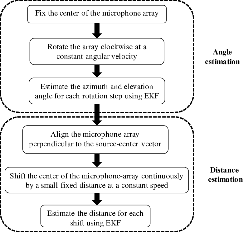
The estimation for the angles and distance of the sound source is conducted by extended Kalman filters. Detailed mathematical derivation of the EKF can be found in BeardMcLain2012. Algorithm 0.2 summaries the EKF procedure used in this paper for SSL. The sensor covariance matrix ($R$) is defined as $\sigma_{w}^{2}$, and the process covariance matrix ($Q$) is defined as $\sigma_{v}^{2}$ for the distance localization, $\sigma_{v1}^{2}$ for the 2D orientation localization and $\text{diag}\{\sigma_{v1}^{2},\sigma_{v2}^{2}\}$ for the 3D orientation localization, respectively, where $\sigma_{vi}$ is the process noise variance corresponding to the $i^{th}$ state and $\sigma_{w}$ is the sensor noise variance. Key parameters are listed in Table 1. The complete EKF-based SSL procedure is illustrated in Figure 13.

7 Simulation Results

In this section, we present the simulation results of the proposed localization technique for both angle and distance localization of a sound source.

7.1 Simulation Environment

The Audio Array Toolbox Donohue2009 is used to simulate a rectangular space using the image method described in allen1979image. The robot was placed in the center (origin) of the room. The two microphones were separated by a distance of $0.18\;\text{m}$ from each other which is equal to the approximate distance between human ears. The sound source and the microphones are assumed omnidirectional and the attenuation of the sound is calculated as per the specifications in Table 2.

Table 2: Simulated room specifications

Parameter	Value
Dimension	20m x 20m x 20m
Reflection coefficient of each wall	0.5
Reflection coefficient of the floor	0.5
Reflection coefficient of the ceiling	0.5
Velocity of the sound	345 m/s
Temperature	22${}^{o}C$
Static pressure	29.92 mmHg
Relative humidity	38 %

7.2 Validation of Observablity

As discussed earlier, Theorem 3.1 shows that the 2D model is always observable, however, it does not provides any elevation information of the sound source. On the other hand, Theorem 3.2 shows that the 3D model is unobservable when the elevation angle of the sound source is $0^{o}$ or $90^{o}.$ In order to validate the observability analysis, localization was performed in the simulated environment.

For a sound source located on a 2D plane, Figure 14 shows the average of absolute estimation errors versus different azimuth angles with the sound source at distance of $5\;\text{m}$ and $10\;\text{m}$ to the robot, respectively. It can be seen that all errors are smaller than $1.8^{o}$ and the mean of the average of absolute errors is approximately $1^{o}$ for the two cases.

Figure 14: Average of absolute errors in azimuth angle estimation using 2D model with a sound source placed at different azimuth locations at a constant distance of 5 m and 10 m from the center of the robot.

Figure 15: Sound source locations with a fixed distance of 5 m to the center of the robot in the simulated room.

Figure 16: Average of absolute errors in elevation estimation using the 3D localization model. Relatively large errors illustrate the non-observability condition in elevation angle estimation with sound source placed around $0^{o}$ elevation, as described by Theorem 3.2 .

Figure 17: Average of absolute errors in azimuth estimation using the 3D localization model. Relatively large errors illustrate the non-observability condition in azimuth angle estimation with sound source placed around $90^{o}$ elevation, as described by Theorem 3.2 .

To verify the observability conditions for the 3D model as described by Equations (3.3) and (14), the sound source is placed at different locations with a distance of $5\;\text{m}$ from the robot in the simulated room, which evenly cover the hemisphere above the ground, as shown in Figure 15. Figure 16 shows the averaged absolute errors in the elevation estimation versus actual azimuth and elevation angles of the sound source. Larger errors were observed when the elevation was close to $0^{o}$, which coincides with Theorem 3.2. Figure 17 shows the averaged absolute errors in the azimuth angle estimation for a single sound source at different positions. Larger errors were observed when the elevation was close to $90^{o}$, which again echoes Theorem 3.2.

7.3 Simulation Results for Orientation Localization

Table 3: Simulation results of orientation localization for speech

Expt.	Act.	Act.	Est.	Avg of abs	Act.	Est.	Avg of abs
No.	D(m)	$\varphi$(o)	$\varphi$(o)	error (o)	$\theta$(o)	$\theta$(o)	error (o)
1 a	5	0	0.60	0.60	20	20.39	0.39
1 b	5	50	51.03	1.03		21.44	1.44
1 c	7	90	91.21	0.21		20.83	0.83
1 d	7	120	121.57	1.57		20.96	0.96
1 e	3	180	181.03	1.03		20.16	0.16
1 f	3	-40	-39.33	0.67		19.10	0.90
1 g	10	-90	-88.85	1.15		21.66	1.66
1 h	10	-140	-139.52	0.48		21.18	1.18
2 a	5	0	2.31	2.31	60	60.68	0.68
2 b	5	50	50.65	0.65		60.53	0.53
2 c	7	90	91.79	1.79		60.70	0.70
2 d	7	120	121.85	1.85		60.84	0.84
2 e	3	180	181.66	1.66		60.05	0.05
2 f	3	-40	-38.66	1.34		60.38	0.38
2 g	10	-90	-89.38	0.62		59.62	0.38
2 h	10	-140	-138.20	1.80		59.78	0.22
3 a	5	50	50.69	0.31	0	3.39	3.39
3 b	7	-120	-119.00	1.00	4	2.40	1.60
4 a	5	-40	not def.	not def.	86	90.00	4.00
4 b	7	150	not def.	not def.	89	90.00	1.00

Table 4: Simulation results of orientation localization for white noise

Expt.	Act.	Act.	Est.	Avg of abs	Act.	Est.	Avg of abs
No.	D(m)	$\varphi$(o)	$\varphi$(o)	error (o)	$\theta$(o)	$\theta$(o)	error (o)
1 a	5	0	1.18	1.18	20	19.66	0.34
1 b	5	50	51.03	1.03		20.44	0.44
1 c	7	90	90.25	0.25		20.11	0.11
1 d	7	120	121.35	1.35		19.70	0.30
1 e	3	180	180.41	0.41		20.48	0.48
1 f	3	-40	-39.44	0.56		19.75	0.25
1 g	10	-90	-89.11	0.89		19.71	0.29
1 h	10	-140	-139.67	0.33		21.18	1.18
2 a	5	0	1.31	1.31	60	60.38	0.38
2 b	5	50	51.59	1.59		60.39	0.39
2 c	7	90	90.74	0.74		60.87	0.87
2 d	7	120	121.21	1.21		60.39	0.39
2 e	3	180	181.16	1.16		60.51	0.51
2 f	3	-40	-38.66	1.34		60.41	0.41
2 g	10	-90	-88.90	1.10		60.70	0.70
2 h	10	-140	-138.64	1.36		60.57	0.57
3 a	5	50	51.45	1.45	0	1.57	1.57
3 b	7	-120	-118.36	1.64	4	1.57	2.43
4 a	5	-40	not def.	not def.	86	90.00	4.00
4 b	7	150	not def.	not def.	89	90.00	1.00

A number of experiments were performed to validate the performance of the proposed SSL technique for orientation localization, as described in Algorithm 0.1. White noise and speech signals were used as a sound source which was placed individually at different locations in the simulated room with specifications summarized in Table 2. The microphone array was rotated with an angular velocity of $\omega=2\pi/5$ rad/sec in the clockwise direction for three complete revolutions. The ITD was calculated after every $1^{o}$ rotation followed by the estimation performed using the EKF with parameters given in Table 1. Four different sets of experiments were performed keeping the source at different locations. In first two sets of experiments, the source was placed in all four quadrants including the axes at different distances, keeping the elevation constant at $20^{o}$ and $60^{o}$. To validate the performance of the proposed solution to the non-observability conditions, other two sets experiments were performed by keeping the sound source at elevation close to $0^{o}$ and $90^{o}$. The results of the localization are presented in Tables 3 and 4. It can be seen that orientation localization is achieved with errors less than $4^{o}$ using speech as well as white noise sound source. Large errors are observed when the elevation of the sound source is around $0^{o}$ and $90^{o}$. Further, the errors with source elevation around $0^{o}$ is less as compared to source elevation around $90^{o}$. This was achieved by using polynomial curve fitting approach mentioned in Section 4.2, with $RMSE_{threshold}=1.9^{o}$, which corresponds to $\theta=15^{o}$ on the fitted curve shown in Figure 9 . The value $d_{threshold}$ was calculated as $0.017$ m (which corresponds to $\theta=85^{o}$, thereby giving an accuracy of $5^{o}$ when the sound source gets close to $90^{o}$ elevation) for the simulated environment with specification given in Table 2.

7.4 Simulation Results for Distance Localization

Table 5: Simulation results of distance localization using speech sound source

Expt.	Act.	Act.	Act.	Est.	Avg of abs
No.	$\varphi$(o)	$\theta$(o)	D(m)	D(m)	error (m)
1 a	0	20	5	5.01	0.01
1 b	50		5	5.01	0.01
1 c	90		7	6.94	0.06
1 d	120		7	6.93	0.07
1 e	180		3	3.01	0.01
1 f	-40		3	3.01	0.01
1 g	-90		10	9.54	0.46
1 h	-140		10	9.81	0.19
2 a	0	60	5	5.02	0.02
2 b	50		5	5.02	0.02
2 c	90		7	6.94	0.06
2 d	120		7	6.94	0.06
2 e	180		3	3.00	0.00
2 f	-40		3	3.01	0.01
2 g	-90		10	9.52	0.48
2 h	-140		10	9.41	0.59
3 a	50	0	5	5.02	0.02
3 b	-120	4	7	6.87	0.13
4 a	-40	86	5	5.02	0.02
4 b	150	89	7	6.83	0.17

Table 6: Simulation results of distance localization using white noise sound source

Expt.	Act.	Act.	Act.	Est.	Avg of abs
No.	$\varphi$(o)	$\theta$(o)	D(m)	D(m)	error (m)
1 a	0	20	5	5.01	0.01
1 b	50		5	5.01	0.01
1 c	90		7	6.92	0.08
1 d	120		7	6.92	0.08
1 e	180		3	3.01	0.01
1 f	-40		3	3.01	0.01
1 g	-90		10	9.52	0.48
1 h	-140		10	9.44	0.56
2 a	0	60	5	5.01	0.01
2 b	50		5	5.01	0.01
2 c	90		7	6.92	0.08
2 d	120		7	6.92	0.08
2 e	180		3	3.01	0.01
2 f	-40		3	3.01	0.01
2 g	-90		10	9.48	0.52
2 h	-140		10	9.43	0.57
3 a	50	0	5	5.01	0.01
3 b	-120	4	7	6.89	0.11
4 a	-40	86	5	5.01	0.01
4 b	150	89	7	6.90	0.10

Figure 18: Simulation results for distance estimation using EKF. A single sound source was placed at two different locations with distances of $5$ m and $10$ m, respectively. The bounds represent the three standard deviation of the estimation error.

Speech and white-noise sounds were also used to test the performance of the distance localization. A single sound source was placed at different locations and the ITD signal was recorded while the microphone array was continuously shifted for $200$ steps each with a distance of $\triangle d=0.0007$ m. The results are summarized in Tables 5 and 6. The key parameters of the EKF are given in Table 1. The results for the distance localization with a sound source placed at different locations are shown in Figure 18. It is observed that the error in the estimation converges quickly and a total shift of microphone array of approximately $3\text{ \text{cm}}$ is sufficient for the estimates to completely converge to and remain in the three standard deviation bounds. The average of absoute error in the estimation is found to be less than $0.6$ m in both the case of speech as well as white noise sound sources.

8 Experimental Results

Experiments were conducted using two different hardware platforms: a KEMAR dummy head in a well equipped hearing laboratory and a robotic platform equipped with a set of two rotational microphones. The following subsections discuss the hardware platforms and the results.

8.1 Results using KEMAR Dummy Head

Experiments using the KEMAR dummy head were conducted in a high frequency focused sound treated room yost2014sound with dimension $4.6\text{ }\text{m}$ x $3.7\text{ }\text{m}$ x $2.7\text{ }\text{m}$ as shown in Figure 19. The ITD however is mostly effective for low frequency sounds below 1.5 kHz as a spatial hearing cue middlebrooks1991sound. The walls, floor, and ceiling of the room were covered by polyurethane acoustic foam with a thickness of only 5 cm which is relatively low compared to the sound wavelength thereby making a relatively low reduction in low and middle frequencies beranek2012acoustics, thereby making it a challenging acoustic environment. For broad band noise, T60 (i.e., the time required for the sound level to decay 60 dB Sabine1922) was 97 ms. In an octave band centered at 1000 Hz, T60 for the noise was on an average of 324 ms.

Figure 19: Setup of the KEMAR dummy head on a rotating chair in the middle of the sound treated room Sun2015.

The digitally generated audio signals using a MATLAB program and three 12-channel Digital-to-Analog converters running at 44,100 cycles each second per channel were amplified using AudioSource AMP 1200 amplifiers before they were played from an array of 36 loudspeakers. The two microphones were installed on the KEMAR dummy head temporarily mounted on a rotating chair which was rotated at an approximate rate of 32°/s for about two circles in the middle of the room. The data collected in the second rotation was used for the EKF. Motion data was collected by the gyroscope mounted on the top of the dummy head. The audio signals were amplified and collected by a sound card which were then stored on a desktop computer for further processing. The ITD was processed with a generalized cross-correlation model Knapp1976The in each time frame corresponding to the 120 Hz sampling rate of the gyroscope. The computation was completed by a MATLAB program on a desktop computer. Raw data with a single sound source located at four different locations were collected.

Figure 20: Experimental results for orientation localization using the KEMAR dummy head. When $\theta=0^{o}$, the azimuth estimates using the 2D and 3D models are very close (in the top-left figure), which implies the elevation estimates are not reliable (in the bottom-left figure). When $\theta=30^{o}$, the azimuth estimates are obviously different (in the top-right figure), which implies reliable elevation estimates using the 3D model (in the bottom-right figure).

The left two subfigures in Figure 20 are generated when the actual elevation angle is $0^{o}$. It can be seen that the azimuth estimations using the 2D and 3D models are very close, which implies that the actual elevation angle is close to $0^{o}$ and the elevation estimation using the 3D model is not reliable. The right two subfigures in Figure 20 are generated when the actual elevation angle is $30^{o}$. It can be seen that the azimuth estimations using the 2D and 3D localization models are obviously different while the elevation estimation using the 3D model is fairly accurate, which verifies the proposed algorithm shown in Figure 10. Table 7 shows the estimation results obtained using the 3D localization model. It can be seen that the RMSE of the difference between the estimated azimuth values using respectively the 2D and 3D models works well in checking the zero elevation condition.

Table 7: Experimental results using KEMAR dummy head: Orientation localization using the 3D model. (RMSE: difference between azimuth estimations using the 2D and 3D models, respectively)

Expt.	Act.	Est.	Avg of abs	RMSE	Act.	Est.	Avg of abs
No.	$\varphi$(o)	$\varphi$(o)	error (o)	(o)	$\theta$(o)	$\theta$(o)	error (o)
1	90	91.21	1.21	1.39	0	13.64	13.64
2	-20	-21.53	1.53	1.16	0	48.14	48.14
3	90	90.40	0.40	79.94	60	59.05	0.95

8.2 Results using Robotic Platform

Experiments were also performed using a robotic platform shown in Figure 21. In these experiments, two microelectromechanical systems (MEMS) analog/digital microphones were used for recording the sound signal coming from the sound source. Flex adapters were used to hold the microphones. The angular speed of the rotation of the microphone array was controlled by a bipolar stepper motor with gear ratio adjusted to $0.9^{o}$ per step. The stepper motor was controlled by an Arduino microprocessor. The distance between two microphones was kept constant as $0.3\text{ }\text{m}$. An audio (music) was played in a loud speaker which was used as a sound source kept at different locations. The estimation results are shown in Figure 22 and Table 8.

Figure 21: A two-microphone system is equipped on a ground robot.

Figure 22: Experimental results for orientation localization using the robotic platform. When $\theta=0^{o}$, the azimuth estimates using the 2D and 3D models are very close (in the top-left figure), which implies the elevation estimates are not reliable (in the bottom-left figure). When $\theta=55^{o}$, the azimuth estimates are obviously different (in the top-right figure), which implies reliable elevation estimates using the 3D model (in the bottom-right figure).

Table 8: Experimental results using the robotic platform: Orientation localization using 3D model (RMSE: difference between azimuth estimations using the 2D and 3D models, respectively)

Expt.	Act.	Est.	Avg of abs	RMSE	Act.	Est.	Avg of abs
No.	$\varphi$(o)	$\varphi$(o)	error (o)	(o)	$\theta$(o)	$\theta$(o)	error (o)
1	-140	-140.65	0.65	0.72	0	14.96	14.96
2	180	178.71	1.29	0.69	5	11.59	6.59
3	40	39.67	0.33	8.80	55	55.24	0.24
4	40	38.20	1.80	10.96	65	64.67	0.33

It can be seen that the azimuth estimations using the 2D and 3D models shown in the top-left subfigure in Figure 22 generated when the actual elevation angle is $0^{o}$ are very close, which implies that the elevation is close to $0^{o}$ and the elevation estimation shown in the bottom-left subfigure in Figure 22 using the 3D localization model is not reliable. However, the two subfigures on the right in Figure 22 are generated by keeping the sound source at an elevation angle of $55^{o}$. As proposed in the algorithm shown in Figure 10, the azimuth estimations using the 2D and 3D localization models are different while the elevation estimation using the 3D model is fairly accurate. Table 8 shows the estimation results obtained using the 3D localization model. It can be seen that the zero elevation condition can be checked using the RMSE of the difference between the estimated azimuth values using respectively the 2D and 3D models.

A fitted curve similar to one shown in the Figure 9 can be generated for the environment by keeping the sound source at different elevation angles and recording the $RMSE$ values between $\varphi_{2D}$ and $\varphi_{3D}$ estimations. The value of the parameter $RMSE_{threshold}$ can be decided, which can be used to check the $\theta=0^{o}$ scenario. Further, the generated fitted curve can be used to give a closer estimation of the elevation angle.

9 Conclusion

This paper presents a novel technique that performs a complete localization (i.e., both orientation and distance) of a stationary sound source in a three-dimensional (3D) space. Two singular conditions when unreliable orientation localization (the elevation angle equals $0$ or $90^{o}$) occurs were found by using the observability theory. The root-mean-squared error (RMSE) value of the difference between the azimuth estimates using respectively the 2D and 3D models was used to check the $0^{o}$ elevation condition and the elevation was further estimated using a polynomial curve fitting technique. The $90^{o}$ elevation was detected by checking zero-ITD signal. Based on an accurate orientation localization, the distance localization was done by first rotating the microphone array to face toward the sound source and then shifting the microphones perpendicular to the source-robot vector by a distance of a fixed number of steps. Under challenging acoustic environments with relatively low-energy targets and high-energy noise, high localization accuracy was achieved in both simulations and experiments. The mean of the average of absolute estimation error was less than $4^{o}$ for angular localization and less than $0.6$ m for distance localization in simulation results and techniques to detect $\theta=0^{o}$ and $90^{o}$ are verified in both simulation and experimental results.

The authors would like to thank Dr. Xuan Zhong for providing with the experimental raw data using the KEMAR dummy head.

References

- (1) International Organization for Standardization (ISO), British, European and International Standards (BSEN), Noise emitted by machinery and equipment – Rules for the drafting and presentation of a noise test code. 12001: 1997 Acoustics
- (2) Allen, J.B., Berkley, D.A.: Image method for efficiently simulating small-room acoustics. The Journal of the Acoustical Society of America 65(4), 943–950 (1979). doi:10.1121/1.382599
- (3) Azaria, M., Hertz, D.: Time delay estimation by generalized cross correlation methods. IEEE Transactions on Acoustics, Speech, and Signal Processing 32(2), 280–285 (1984). doi:10.1109/TASSP.1984.1164314
- (4) Beard, R., McLain, T.: Small Unmanned Aircraft: Theory and Practice. Princeton University Press (2012)
- (5) Benesty, J., Chen, J., Huang, Y.: Microphone array signal processing, vol. 1. Springer Science & Business Media (2008). doi:10.1007/978-3-540-78612-2
- (6) Beranek, L.L., Mellow, T.J.: Acoustics: sound fields and transducers. Academic Press (2012)
- (7) Blumrich, R., Altmann, J.: Medium-range localisation of aircraft via triangulation. Applied Acoustics 61(1), 65–82 (2000). doi:10.1016/S0003-682X(99)00066-3
- (8) Boll, S.: Suppression of acoustic noise in speech using spectral subtraction. IEEE Transactions on Acoustics, Speech, and Signal Processing 27(2), 113–120 (1979). doi:10.1109/TASSP.1979.1163209
- (9) Boll, S., Pulsipher, D.: Suppression of acoustic noise in speech using two microphone adaptive noise cancellation. IEEE Transactions on Acoustics, Speech, and Signal Processing 28(6), 752–753 (1980). doi:10.1109/TASSP.1980.1163472
- (10) Borenstein, J., Everett, H., Feng, L.: Navigating mobile robots: systems and techniques. A K Peters Ltd. (1996)
- (11) Brandes, T.S., Benson, R.H.: Sound source imaging of low-flying airborne targets with an acoustic camera array. Applied Acoustics 68(7), 752–765 (2007). doi:10.1016/j.apacoust.2006.04.009
- (12) Brandstein, M., Ward, D.: Microphone arrays: signal processing techniques and applications. Springer Science & Business Media (2013). doi:10.1007/978-3-662-04619-7
- (13) Brassington, G.: Mean absolute error and root mean square error: which is the better metric for assessing model performance? In: EGU General Assembly Conference Abstracts, vol. 19, p. 3574 (2017)
- (14) Calmes, L.: Biologically inspired binaural sound source localization and tracking for mobile robots. Ph.D. thesis, RWTH Aachen University (2009)
- (15) Chen, J., Benesty, J., Huang, Y.: Time delay estimation in room acoustic environments: an overview. EURASIP Journal on applied signal processing pp. 170–170 (2006). doi:10.1155/ASP/2006/26
- (16) Donohue, K.D.: Audio array toolbox. [Online] Available: http://vis.uky.edu/distributed-audio-lab/about/ , 2017, Dec 22
- (17) Gala, D., Lindsay, N., Sun, L.: Three-dimensional sound source localization for unmanned ground vehicles with a self-rotational two-microphone array. In: Proceedings of the 5th International Conference of Control, Dynamic Systems, and Robotics (CDSR’18). Accepted (2018)
- (18) Gala, D.R., Misra, V.M.: SNR improvement with speech enhancement techniques. In: Proceedings of the International Conference and Workshop on Emerging Trends in Technology, ICWET ’11, pp. 163–166. ACM (2011). doi:10.1145/1980022.1980058
- (19) Gala, D.R., Vasoya, A., Misra, V.M.: Speech enhancement combining spectral subtraction and beamforming techniques for microphone array. In: Proceedings of the International Conference and Workshop on Emerging Trends in Technology, ICWET ’10, pp. 163–166 (2010). doi:10.1145/1741906.1741938
- (20) Gill, D., Troyansky, L., Nelken, I.: Auditory localization using direction-dependent spectral information. Neurocomputing 32, 767–773 (2000). doi:10.1016/S0925-2312(00)00242-3
- (21) Goelzer, B., Hansen, C.H., Sehrndt, G.: Occupational exposure to noise: evaluation, prevention and control. World Health Organisation (2001)
- (22) Goldstein, E.B., Brockmole, J.: Sensation and perception. Cengage Learning (2016)
- (23) Hedrick, J.K., Girard, A.: Control of nonlinear dynamic systems: Theory and applications. Controllability and observability of Nonlinear Systems p. 48 (2005)
- (24) Hermann, R., Krener, A.: Nonlinear controllability and observability. IEEE Transactions on Automatic Control 22(5), 728–740 (1977). doi:10.1109/TAC.1977.1101601
- (25) Hornstein, J., Lopes, M., Santos-Victor, J., Lacerda, F.: Sound localization for humanoid robots-building audio-motor maps based on the HRTF. In: IEEE/RSJ International Conference on Intelligent Robots and Systems (IROS), pp. 1170–1176 (2006). doi:10.1109/IROS.2006.281849
- (26) Huang, Y., Benesty, J., Elko, G.W.: Passive acoustic source localization for video camera steering. In: IEEE International Conference on Acoustics, Speech, and Signal Processing, vol. 2, pp. II909–II912 (2000). doi:10.1109/ICASSP.2000.859108
- (27) Kaushik, B., Nance, D., Ahuja, K.: A review of the role of acoustic sensors in the modern battlefield. In: 11th AIAA/CEAS Aeroacoustics Conference (2005). doi:10.2514/6.2005-2997
- (28) Keyrouz, F.: Advanced binaural sound localization in 3-D for humanoid robots. IEEE Transactions on Instrumentation and Measurement 63(9), 2098–2107 (2014). doi:10.1109/TIM.2014.2308051
- (29) Keyrouz, F., Diepold, K.: An enhanced binaural 3D sound localization algorithm. In: IEEE International Symposium on Signal Processing and Information Technology, pp. 662–665 (2006). doi:10.1109/ISSPIT.2006.270883
- (30) Knapp, C., Carter, G.: The generalized correlation method for estimation of time delay. IEEE Transactions on Acoustics, Speech, and Signal Processing 24(4), 320–327 (1976). doi:10.1109/TASSP.1976.1162830
- (31) Kumon, M., Uozumi, S.: Binaural localization for a mobile sound source. Journal of Biomechanical Science and Engineering 6(1), 26–39 (2011). doi:10.1299/jbse.6.26
- (32) Laurent Kneip, C.B.: Binaural model for artificial spatial sound localization based on interaural time delays and movements of the interauralaxis. The Journal of the Acoustical Society of America pp. 3108–3119. (2008). doi:10.1121/1.2977746
- (33) Lu, Y.C., Cooke, M.: Motion strategies for binaural localisation of speech sources in azimuth and distance by artificial listeners. Speech Communication 53(5), 622–642 (2011). doi:10.1016/j.specom.2010.06.001
- (34) Lu, Y.C., Cooke, M., Christensen, H.: Active binaural distance estimation for dynamic sources. In: INTERSPEECH, pp. 574–577 (2007)
- (35) Middlebrooks, J.C., Green, D.M.: Sound localization by human listeners. Annual review of psychology 42(1), 135–159 (1991). doi:10.1146/annurev.ps.42.020191.001031
- (36) Naylor, P., Gaubitch, N.D.: Speech dereverberation. Springer Science & Business Media (2010). doi:10.1007/978-1-84996-056-4
- (37) Nguyen, Q.V., Colas, F., Vincent, E., Charpillet, F.: Long-term robot motion planning for active sound source localization with Monte Carlo tree search. In: Hands-free Speech Communications and Microphone Arrays (HSCMA), pp. 61–65 (2017). doi:10.1109/HSCMA.2017.7895562
- (38) Omologo, M., Svaizer, P.: Acoustic source location in noisy and reverberant environment using csp analysis. In: IEEE International Conference on Acoustics, Speech, and Signal Processing Conference, vol. 2, pp. 921–924 (1996). doi:10.1109/ICASSP.1996.543272
- (39) Pang, C., Liu, H., Zhang, J., Li, X.: Binaural sound localization based on reverberation weighting and generalized parametric mapping. IEEE/ACM Transactions on Audio, Speech, and Language Processing 25(8), 1618–1632 (2017). doi:10.1109/TASLP.2017.2703650
- (40) Perrett, S., Noble, W.: The effect of head rotations on vertical plane sound localization. The Journal of the Acoustical Society of America 102(4), 2325–2332 (1997). doi:10.1121/1.419642
- (41) Rodemann, T.: A study on distance estimation in binaural sound localization. In: IEEE/RSJ International Conference on Intelligent Robots and Systems (IROS), pp. 425–430 (2010). doi:10.1109/IROS.2010.5651455
- (42) Rodemann, T., Ince, G., Joublin, F., Goerick, C.: Using binaural and spectral cues for azimuth and elevation localization. In: IEEE/RSJ International Conference on Intelligent Robots and Systems (IROS), pp. 2185–2190 (2008). doi:10.1109/IROS.2008.4650667
- (43) Sabine, W.: Collected Papers on Acoustics. Harvard University Press (1922)
- (44) Spriet, A., Van Deun, L., Eftaxiadis, K., Laneau, J., Moonen, M., Van Dijk, B., Van Wieringen, A., Wouters, J.: Speech understanding in background noise with the two-microphone adaptive beamformer beam in the nucleus freedom cochlear implant system. Ear and hearing 28(1), 62–72 (2007). doi:10.1097/01.aud.0000252470.54246.54
- (45) Sturim, D.E., Brandstein, M.S., Silverman, H.F.: Tracking multiple talkers using microphone-array measurements. In: IEEE International Conference on Acoustics, Speech, and Signal Processing, vol. 1, pp. 371–374 vol.1 (1997). doi:10.1109/ICASSP.1997.599650
- (46) Sun, L., Zhong, X., Yost, W.: Dynamic binaural sound source localization with interaural time difference cues: Artificial listeners. The Journal of the Acoustical Society of America 137(4), 2226–2226 (2015). doi:10.1121/1.4920636
- (47) Tamai, Y., Kagami, S., Amemiya, Y., Sasaki, Y., Mizoguchi, H., Takano, T.: Circular microphone array for robot’s audition. In: Proceedings of IEEE Sensors, 2004., vol. 2, pp. 565–570 (2004). doi:10.1109/ICSENS.2004.1426228
- (48) Tamai, Y., Sasaki, Y., Kagami, S., Mizoguchi, H.: Three ring microphone array for 3D sound localization and separation for mobile robot audition. In: IEEE/RSJ International Conference on Intelligent Robots and Systems (IROS), pp. 4172–4177 (2005). doi:10.1109/IROS.2005.1545095
- (49) Tiete, J., Domínguez, F., Silva, B.d., Segers, L., Steenhaut, K., Touhafi, A.: Soundcompass: a distributed MEMS microphone array-based sensor for sound source localization. Sensors 14(2), 1918–1949 (2014). doi:10.3390/s140201918
- (50) Valin, J.M., Michaud, F., Rouat, J., Letourneau, D.: Robust sound source localization using a microphone array on a mobile robot. In: IEEE/RSJ International Conference on Intelligent Robots and Systems (IROS), vol. 2, pp. 1228–1233 (2003). doi:10.1109/IROS.2003.1248813
- (51) Wallach, H.: On sound localization. The Journal of the Acoustical Society of America 10(4), 270–274 (1939). doi:10.1121/1.1915985
- (52) Wang, H., Chu, P.: Voice source localization for automatic camera pointing system in videoconferencing. In: IEEE International Conference on Acoustics, Speech, and Signal Processing, vol. 1, pp. 187–190 (1997). doi:10.1109/ICASSP.1997.599595
- (53) Yost, W.A., Zhong, X.: Sound source localization identification accuracy: Bandwidth dependencies. The Journal of the Acoustical Society of America 136(5), 2737–2746 (2014). doi:10.1121/1.4898045
- (54) Zhong, X., Sun, L., Yost, W.: Active binaural localization of multiple sound sources. Robotics and Autonomous Systems 85, 83–92 (2016). doi:10.1016/j.robot.2016.07.008
- (55) Zhong, X., Yost, W., Sun, L.: Dynamic binaural sound source localization with ITD cues: Human listeners. The Journal of the Acoustical Society of America 137(4), 2376–2376 (2015). doi:10.1121/1.4920636
- (56) Zietlow, T., Hussein, H., Kowerko, D.: Acoustic source localization in home environments-the effect of microphone array geometry. In: 28th Conference on Electronic Speech Signal Processing, pp. 219–226 (2017)