Universal Noise in Continuous Transport Measurements of Interacting Fermions

Abstract

We propose and analyze continuous measurements of atom number and atomic currents using dispersive measurements in an optical cavity. For an atom-number measurement in a closed system, we relate both the detection noise and the heating rate due to measurement back-action to Tan’s contact, and demonstrate an emergent universal quantum non-demolition (QND) regime in the good cavity limit. We then show that such a continuous QND measurement of atom number serves as a quantum-limited current transducer in the two-terminal setup. We derive a universal bound on precision of current measurement, which results from a tradeoff between detection noise and back-action of the atomic current measurement. Our results apply regardless of interaction strength or phases of matter and set fundamental bounds on future precision measurements of transport properties in cold-atom quantum simulators.

Transport is among the best probes of quantum many-body systems, because it is sensitive to the nature of the system’s excitations. Recently, quantum simulation has emerged as a new method to tackle the many-body problem by using a controlled cold atomic gas as a model for electrons in condensed matter [1]. With this approach getting mature enough to address the open questions of condensed matter physics, there is a growing interest in the direct measurement of transport properties in atomic gases [2, 3]. The current methods used to investigate transport in cold atomic gases suffer from the intrinsically destructive nature of the observation. Even when snapshots of the density distribution is obtained at the level of individual atoms, the investigations of the dynamics involve sample-to-sample fluctuations. As a result, the noise in the preparation directly feeds in the measurement outcomes, rendering the cold-atom transport measurements far less precise than their condensed-matter counterparts. In the latter case, details such as current fluctuations have revealed crucial pieces of information, such as the fractional charge of the excitations [4].

In this Letter, we describe and analyze the continuous measurement of atomic currents on single realizations of a cold atomic gas. The concept is depicted in Fig. 1: it relies on (i) the two (or multi-)terminal configuration, where the system of interest is connected to large atomic reservoirs allowing to inject and collect particles, and (ii) the use of continuous measurements of atom numbers using a high-finesse cavity and a probe laser far from the atomic resonance. The atomic current consists of atoms continuously entering and leaving the reservoir, thereby interacting with the cavity mode and causing the phase shift of a probe laser, which is measured by a quantum-limited interferometer. The high-finesse cavity ensures that the phase shift and the measurement back-action stand out of the effects of spontaneous emission [5, 6].

Figure 1: Experimental concept of the atomic current detector. An atomic cloud is shaped in a two-terminal setup with large reservoirs connected by a mesoscopic channel. One reservoir overlaps with the mode of a single-sided optical cavity. A chemical potential difference introduced between the two reservoirs drives a quasi-DC current in the channel. A probe beam far detuned from the atomic resonance is sent onto the cavity, and its phase, measured by homodyne detection, provides a real-time measurement of the atom number in the reservoir.

We first investigate a continuous dispersive measurement of a reservoir in the absence of currents, and show that both the interferometer noise spectrum and the heating due to measurement back-action are universally expressed in terms of Tan’s contact, which is the parameter describing the two-body correlations at short distances [7] and relates the macroscopic properties to the two-body problem, regardless of phases of matter or temperature [8]. The connection between Tan’s contact and measurement back action provides a quantitative estimate of the measurement outcomes, and allows one to identify a good cavity limit where the universal back-action vanishes regardless of the interaction strength, realizing an emergent QND measurement for the many-body system. This complements existing proposals focusing on single particle physics or lattice systems [9, 10, 11, 12, 13, 14, 15].

We then consider the connection between the reservoir and the channel, where the reservoir population operator no longer commutes with the Hamiltonian of the full system. Therefore, even in the good cavity limit, the continuous measurement yields a finite back-action on the transport process itself which we interpret as fluctuations of the chemical potential bias across the channel. Together with the intrinsic interferometric detection noise, this back-action yields a universal quantum limit on the precision of the atomic current measurement, which we derive explicitly in terms of the finite-bias admittance of the channel. Our approach does not assume Fermi liquid behavior nor linear response of the atomic current to the applied bias, even though the atom-field coupling is treated within linear response theory.

Continuous reservoir observation.— We first consider a closed reservoir containing $N$ Fermions at zero temperature, dispersively coupled to the optical field in a Fabry-Perot cavity which, in turn, is coupled to an environment through an imperfect mirror. The field is far detuned from the atomic resonances, such that the excited states of the atoms are not populated. The atoms populate equally two hyperfine states, and for simplicity we assume these two states to be coupled identically to the field, though this hypothesis is not essential. Then the Hamiltonian of the system reads [16]

$$\hat{H}=\hat{H}_{at}+\omega_{c}\hat{d}^{\dagger}\hat{d}+\Omega\hat{M}\hat{d}^{\dagger}\hat{d},$$ (1)

Here $\hat{H}_{at}$ is the Hamiltonian of the atoms in the absence of the cavity field, consisting of the kinetic energy, interactions between the two spin components and a possible trapping potential. The empty cavity has frequency $\omega_{c}$, and $\hat{d}$ ($\hat{d}^{\dagger}$) annihilate (create) photons in the cavity. The coupling $\Omega$ of the atoms to the field represents the shift of the cavity resonance due to the presence of one atom maximally coupled to the field, and $\hat{M}$ is the overlap of the density distribution of the atoms with the cavity mode:

$$\hat{M}=\int d\mathbf{r}\cos^{2}(kz)\hat{n}(\mathbf{r})=\frac{1}{2}\hat{N}+\frac{1}{4}(\hat{n}_{2k}+\hat{n}_{-2k}),$$ (2)

where $k$ is the wave vector of the cavity photons. We have introduced the operators for the total atom density $\hat{n}(\mathbf{r})$, the total atom number $\hat{N}$ and the density fluctuations $\hat{n}_{2k}=\int d\mathbf{r}e^{-2ikz}\hat{n}(\mathbf{r})$. Here we consider a situation in which the waist of the cavity mode is much larger than the atomic cloud.

We describe a coherent driving resonant with the cavity and the coupling to the vacuum using the input-output formalism [17]. We decompose the atom-field coupling into a non-fluctuating part which we suppose is included in $\hat{H}_{at}$ , and a part containing the vacuum fluctuations $\hat{\eta}$. To first order in $\hat{\eta}$, the coupling Hamiltonian reads $\hat{F}\hat{M}$, where $\hat{F}=ig(\hat{\eta}^{\dagger}-\hat{\eta})$ with $g=2\Omega\sqrt{\Phi/\kappa}$ being the measurement strength, $\Phi$ is the photon flux incident on the cavity, and $\kappa$ is the cavity decay rate. Importantly, to first order in fluctuations, the time evolution of $\hat{F}$ is decoupled from that of the atoms, so that the freely evolving $\hat{F}(t)$ can be directly treated as a perturbation for the atoms.

The presence of the operators $\hat{n}_{\pm 2k}$ in $\hat{M}$ implies that $\hat{M}$ does not commute with the atomic Hamiltonian, and that the measurement is thus destructive. In fact, the Heisenberg equation directly relates the commutator of $\hat{M}$ with $\hat{H}_{at}$ to the energy absorption rate due to measurement:

$$\frac{d\hat{H}_{at}}{dt}=-i\left[\hat{H}_{at},\hat{M}\right]\hat{F}.$$ (3)

We evaluate this expression using linear response theory, obtaining [18]

$$\frac{d\mathcal{E}_{\mathrm{at}}}{dt}=-\frac{g^{2}\kappa}{16n}\chi^{R}(2k,i\kappa/2),$$ (4)

where $\mathcal{E}_{\mathrm{at}}$ is the energy per atom, $n$ is the atomic density, and $\chi^{R}$ is the retarded density response function which is determined by an equilibrium average. .

We now specialize in the case with $2k\gg k_{F}$ and $\kappa/2\gg\epsilon_{F}$, which we expect to be realized in typical cold-atom experiments [19, 20, 21, 22] (note however Ref. [23]). In this regime, the density response function can be systematically evaluated using the operator product expansion [24, 25, 26, 27, 28] (OPE), regardless of the interaction strength, temperature, and phase of matter. The result of this expansion is expressed as

$$\frac{1}{g^{2}}\frac{d\mathcal{E}_{\mathrm{at}}}{dt}=g_{n}(x)+g_{c}(x,2ka)\frac{C}{k_{F}^{4}}\left(\frac{k_{F}}{2k}\right)\\ +g_{H}(x)\frac{\mathcal{E}_{\mathrm{at}}}{\mathcal{E}_{0\mathrm{at}}}\left(\frac{k_{F}}{2k}\right)^{2}+...,$$ (5)

where $C$ is Tan’s contact density, $\mathcal{E}_{0\mathrm{at}}=3\epsilon_{F}/5$ is the energy per atom of a noninteracting Fermi gas. The functions $g_{n}$, $g_{c}$, and $g_{H}$ are universal functions of $x=\frac{\kappa m}{4k^{2}}$ and $ka$, where $a$ is the $s$-wave scattering length. The analytic expressions of these universal functions are shown in Ref. [18].

Figure 2: Dimensionless energy absorption rate as functions of $x$ and the interaction parameter $1/(k_{F}a)$. The cuts in red, green and blue present the dimensionless energy absorption rate for $1/(k_{F}a)=-0.5,\,0,$ and $0.5$, respectively.

Figure 2 presents the right-hand side of Eq. (5) for the ratio $k_{F}/(2k)=0.2$, in line with typical experiments using ⁶Li atoms, and well in the valid regime of the OPE [29, 30]. The normalization implies that variations of $x$ (i.e., $\kappa$) are taken at a constant mean intra-cavity photon number. In the limit of large $x$, the heating rate tends to vanish according to a power law, a feature expected from Tan’s relations. In the opposite limit of low $\kappa$ (but large compared with $\epsilon_{F}$), heating linearly decreases to zero, due to the saturation of $\chi$ at low $\omega$. In this regime, the cavity responds too slowly to resolve the atomic motion along the cavity mode, thereby realizing an emergent QND regime [31, 32]. While the OPE fails in the $\kappa\rightarrow 0$ limit, the region of parameters $\epsilon_{F}<\kappa<\epsilon_{2k}$ represents a significant window for a QND operation. As interactions are varied from the BCS to the BEC limit, the maximum shifts towards low frequencies, as a result of pairing becoming more pronounced. Here, we have neglected heating due to spontaneous emission, which is justified for cavities with large enough cooperativities (see  [18] for details).

The input-output formalism predicts that the photocurrent of the homodyne detector can be expressed after appropriate renormalization and up to a constant offset as $I_{h}(t)=\hat{b}_{\mathrm{out}}+\hat{b}^{\dagger}_{\mathrm{out}}$. Here $\hat{b}_{\mathrm{out}}$ describes the field emanating from the cavity, and the phase of the interferometer is chosen to be zero. The mean homodyne current relates to the atom number through $\langle\hat{N}\rangle=\sqrt{\kappa}\langle I_{h}\rangle/2g$. Using again linear response theory, we relate the photocurrent noise spectral density, referred back to the atom number, to the dynamical structure factor $S$ of the gas [18]:

$$\mathcal{S}_{NN}(\omega)=\frac{\kappa}{4g^{2}}+N^{2}\delta(\omega)+\frac{V}{4}\frac{S(2k,\omega)+S(2k,-\omega)}{1+\left(\frac{2\omega}{\kappa}\right)^{2}},$$ (6)

where $V$ is the volume of the system. The first term on the right-hand side shows the imprecision introduced by the photon shot noise, the second term comes from the constant value of $N$, and the last term represents the quantum fluctuations of atoms in the cavity mode. While a similar form of the noise was obtained in a Bose-Einstein condensate inside a cavity from a different perspective [33], we do not rely on the mean-field approximation, and the above formula is valid for any system in the weak atom-field coupling regime.

Similar to the heating rate, the atomic contribution to the noise is also universal in the regime where the OPE is valid. In contrast to the density response at imaginary frequencies, the OPE expansion for the structure factor has been considered in Refs. [25, 26, 27, 28]. In the good cavity regime, the contribution of the atomic fluctuations becomes negligible, since $S$ decreases according to a power law in the low-frequency regime, confirming the emergent QND character of the measurement. Our analysis applies for any interactions between Fermions in the weak-measurement limit. In the opposite, strong-measurement regime, even the non interacting Fermi gas shows large nonlinearities [34, 35, 36].

Current measurements.— We now consider the entire system in the presence of a connection between the reservoirs, which we describe with the following Hamiltonian

$$\hat{H}=\hat{H}_{\mathrm{at,L}}+\hat{H}_{\mathrm{at,R}}+\hat{H}_{\mathrm{t}}+\hat{F}\hat{M},$$ (7)

where we introduce a tunneling Hamiltonian $\hat{H}_{\mathrm{t}}$ [37]. We consider the QND regime for the atom-number measurement and replace $\hat{M}$ by $\hat{N}_{L}/2$, with $\hat{N}_{L}$ being the atom number operator in the left reservoir. The Hamiltonians for the left and right reservoirs are identical to $\hat{H}_{at}$ from the previous part, and $\left[\hat{H}_{\mathrm{at,L}},\hat{N}_{L}\right]=\left[\hat{H}_{\mathrm{at,R}},\hat{N}_{L}\right]=0$. The Heisenberg equation for $\hat{N}_{L}$ reduces to the commutator with the tunneling Hamiltonian, and we suppose that Kirchoff’s law $\dot{\hat{N}}_{L}=\hat{I}_{at}$, where $\hat{I}_{at}$ is the atomic current operator.

In order to describe the back-action of the measurement of $\hat{N}_{L}$, we introduce the phase operator $\hat{\Phi}$ as the generator of infinitesimal changes of the atom number in the left reservoir [37]. By construction, it verifies $\left[\hat{N}_{L},\hat{\Phi}\right]=i$ and its action on states in the atom-number representation is $-i\frac{\partial}{\partial N_{L}}$. For a closed reservoir without the probe, the phase operator evolves according to $\dot{\hat{\Phi}}=\frac{\partial\hat{H}_{\mathrm{at,L}}}{\partial N_{L}}$, as a result of $\left[\hat{H}_{\mathrm{at,L}},\hat{N}_{L}\right]=0$. Provided that the chemical potential in the right reservoir is fixed, the above equation allows one to identify the fluctuations of $\dot{\hat{\Phi}}$ as fluctuations of the chemical potential difference between the reservoirs.

The continuous measurement of the atom number yields noise on the phase as a result of Heisenberg’s uncertainty principle, which we evaluate using the Heisenberg equation:

$$\dot{\hat{\Phi}}=\frac{1}{i}\left[\hat{H}_{\mathrm{at,L}}+\hat{H}_{\mathrm{at,R}}+\hat{H}_{\mathrm{t}},\hat{\Phi}\right]+\frac{1}{2}\hat{F},$$ (8)

where the first term on the right-hand side is the evolution in the absence of measurement including the dynamical effects of the coupling between the reservoirs and the channel, and the last term represents the random fluctuations due to the continuous observation. Owing to the fact that in the weak-measurement regime, $\hat{F}$ is not correlated to the reservoir dynamics, the power spectrum of the phase fluctuations is given by $\mathcal{S}_{\Phi\Phi}(\omega)=\mathcal{S}_{\Phi\Phi}^{0}(\omega)+\frac{\mathcal{S}_{FF}(\omega)}{4^{2}\omega^{2}}$, where $\mathcal{S}_{FF}$ is the noise spectrum of $F$, and $\mathcal{S}_{\Phi\Phi}^{0}(\omega)$ describes the fluctuations in the absence of measurement [38]. For a probe resonant with the cavity in the weak-measurement regime, the dynamical back-action of the measurement vanishes since small changes of the atom number do not change the intra-cavity photon number. The atomic current noise spectrum is then

$$\mathcal{S}_{II}(\omega)=\left|Y(\omega)\right|^{2}\left({}^{2}\omega^{2}\mathcal{S}_{\Phi\Phi}^{0}(\omega)+\frac{\mathcal{S}_{FF}(\omega)}{4}\right),$$ (9)

where we introduce the frequency-dependent admittance of the channel $Y(\omega)$ and the noise spectral density of $\hat{F}$, $\mathcal{S}_{FF}(\omega)$. This assumes that the response of the atomic current to small fluctuations around the average bias is linear, but does not assume the linearity of the current-bias relation itself [38].

Measurements of the current in the setup of Fig. 1 will proceed by measurements of the homodyne signal separated in time by $\tau$, yielding an averaged current observable

$$\hat{i}_{\tau}(t)=\frac{\hat{N}(t+\tau)-\hat{N}(t)}{\tau}=\frac{1}{\tau}\int_{t}^{t+\tau}\hat{I}_{at}(u)du,$$ (10)

where the second equality comes from Kirchoff’s law. We assume that $\tau$ is much larger than both $1/\kappa$ and the dwell time of atoms in the channel. The total imprecision on the current measurement is then given by the sum of the imprecision originating from detection and the measurement back-action,

$$\mathcal{S}_{ii}^{\mathrm{imp}}(\omega)=\mathrm{sinc}^{2}\left(\frac{\omega\tau}{2}\right)\left[\frac{\omega^{2}\kappa}{4g^{2}}+\left|Y(\omega)\right|^{2}\frac{g^{2}}{\kappa}\frac{1}{1+\frac{4\omega^{2}}{\kappa^{2}}}\right],$$ (11)

where, consistently with the emergent QND operation we have dropped the equilibrium fluctuations of the atoms within the cavity mode, and we have expressed $\mathcal{S}_{FF}(\omega)$ in terms of the cavity parameters. This expression represents the tradeoff between noise and back-action as the measurement strength is varied, similar to the standard quantum limit in cavity optomechanics [39, 40].

We illustrate this for the case of a fully open quantum point contact at low bias by using the universal conductance quantum as the low-frequency admittance. The total current imprecision $\delta_{ii}^{2}$ obtained by integrating over the bandwidth $1/\tau$ is presented in Fig. 3. The lower bound on current fluctuations is of the order of $1/\tau$, typically two orders of magnitude below the technical noise of the state-of-the-art cold-atom measurements [41].

Figure 3: Total current imprecision for a fully open quantum point contact over a bandwidth $1/\tau$, as a function of the measurement parameter $g^{2}\tau/\kappa$. The dashed red curve represents the contribution of photon shot noise, while the blue dashed-dotted curve represents the contribution of measurement back-action.

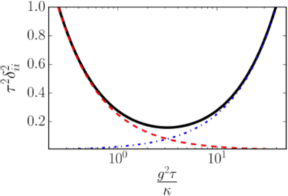
Discussion.— The above result is universal, in that it does not rely on a Fermi liquid description of the reservoirs and thus applies both to the normal and superfluid state of interacting Fermions. It is a consequence of the existence of the emergent QND measurement of a reservoirs population, which is guaranteed regardless of interaction strength by Tan’s relations. It provides a general framework for the quantum simulation of mesoscopic transport using tunable Fermi gases. This concept differs from other proposals where the current operator couples directly with the cavity field via photon-assisted tunneling, which produces a dissipative current [42, 43, 44]. It also differs from mesosopic electronic devices, in that the two terminals together form a closed system, without electromagnetic environments [38], thereby allowing for a simplified and universal analysis.

The most natural experimental platform would consist of cold ⁶Li atoms in the two-terminal configuration accessible in the state-of-the-art experiments [3], where the low mass of the atom facilitates reaching the QND regime. In the presence of a finite $\kappa$ or finite cooperativity, the measurement is not strictly QND. Phenomenologically, we can treat the energy increase in the reservoir as generating a temperature bias across the channel, leading to an extra thermoelectric contribution to the average current [45]. This can be measured to provide a further insight into transport processes, or corrected for a posteriori.

The concept can be generalized to multi-terminal cases, where several cavities or cavity modes monitor several reservoirs simultaneously. Further generalizations could describe situations, where the cavity is focused on a small region within a single cloud in order to observe the dynamics of the gas [32]. In addition, the measurement is, in principle, spin-sensitive such that spin currents as well as particle currents could be monitored along the same principle [46].

We thank C. Galland, T. Donner, and C. Altimiras, T. Giamarchi for discussions and a careful reading of the manuscript, and J. Hofmann and S. Yoshida for discussions on the OPE. JPB acknowledges funding from the ERC project DECCA, EPFL and the Sandoz Family Foundation-Monique de Meuron program for academic promotion. SU is supported by JSPS KAKENHI Grant No. JP17K14366. MU is supported by JSPS KAKENHI Grant No. JP26287088, a Grant-in-Aid for Scientic Research on Innovative Areas “Topological Materials Science” (KAKENHI Grant No. JP15H05855), and the Photon Frontier Network Program from MEXT of Japan.

Supplemental Material

Appendix A Convention

In the input-output formalism, the interaction between the cavity field $\hat{d}$ and bath field $\hat{b}$ is modeled as [17]

$$H_{\text{int}}=i\int_{-\infty}^{\infty}d\omega\kappa(\omega)[\hat{d}\hat{b}^{\dagger}(\omega)-\hat{d}^{\dagger}\hat{b}(\omega)],$$ (12)

where $\hat{b}$ commutes with all system operators such as the cavity and atom fields. When the interaction is the Markov type, which is of our interest, a frequency dependence of the cavity-bath coupling is neglected and we set

$$\kappa(\omega)=\sqrt{\frac{\kappa}{2\pi}}.$$ (13)

The input field is defined in terms of the bath field as follows:

$$\hat{b}_{\text{in}}(t)=\frac{1}{\sqrt{2\pi}}\int_{-\infty}^{\infty}d\omega e^{-i\omega(t-t_{0})}\hat{b}(\omega),$$ (14)

where $t_{0}$ is an initial time. By using the above convention, the Heisenberg equation of motion for the cavity field is obtained as

$$\dot{\hat{d}}=-i\Omega\hat{M}\hat{d}-\frac{\kappa}{2}\hat{d}-\sqrt{\kappa}\hat{b}_{\text{in}}.$$ (15)

In addition, we consider the coherent state input as described by $\hat{b}_{\text{in}}=-i\sqrt{\Phi}+\hat{\xi}$, where $\hat{\xi}$ describes vacuum-field fluctuations. Therefore, combined with the Markov approximation, the vacuum fluctuation field satisfies the following relations:

$$\langle\hat{\xi}(t)\rangle=\langle\hat{\xi}^{\dagger}(t)\rangle=\langle\hat{\xi}^{\dagger}(t)\hat{\xi}(t^{\prime})\rangle=\langle\hat{\xi}(t)\hat{\xi}(t^{\prime})\rangle=0,$$ (16)

$$\langle\hat{\xi}(t)\hat{\xi}^{\dagger}(t^{\prime})\rangle=\delta(t-t^{\prime}).$$ (17)

In the Fourier space, the above expressions can be rewritten as

$$\langle\hat{\xi}(\omega)\rangle=\langle\hat{\xi}^{\dagger}(\omega)\rangle=\langle\hat{\xi}^{\dagger}(\omega)\hat{\xi}(\omega^{\prime})\rangle=\langle\hat{\xi}(\omega)\hat{\xi}(\omega^{\prime})\rangle=0,$$ (18)

$$\langle\hat{\xi}(\omega)\hat{\xi}^{\dagger}(\omega^{\prime})\rangle=2\pi\delta(\omega-\omega^{\prime}).$$ (19)

Appendix B Energy absorption rate

By using the Heisenberg equation of motion, the energy absorption rate is expressed as

$$\frac{dE_{\text{at}}(t)}{dt} = -i\langle[\hat{H}_{\text{at}}(t),\hat{H}(t)]\rangle$$ (20)

$$= -\frac{d}{dt}\langle\hat{M}(t)\hat{F}(t)\rangle-\frac{\kappa}{2}\langle\hat{M}(t)\hat{F}(t)\rangle+2i\Omega\sqrt{\Phi}\langle\hat{M}(t)(\hat{\xi}(t)-\hat{\xi}^{\dagger}(t))\rangle,$$

where we use

$$\frac{d\hat{F}}{dt}=-\frac{\kappa}{2}\hat{F}+2i\Omega\sqrt{\Phi}(\hat{\xi}-\hat{\xi}^{\dagger}).$$ (21)

To proceed with the calculation, we next use the condition that $\hat{F}\hat{M}$ is treated as a perturbation. We then obtain

$$\langle\hat{M}(t)\hat{F}(t)\rangle\approx-i\int_{-\infty}^{t}dt^{\prime}\langle[\hat{M}(t)\hat{F}(t),\hat{M}(t^{\prime})\hat{F}(t^{\prime})]\rangle_{0}$$ (22)

$$\langle\hat{M}(t)(\hat{\xi}(t)-\hat{\xi}^{\dagger}(t))\rangle\approx-i\int_{-\infty}^{t}dt^{\prime}\langle[\hat{M}(t)(\hat{\xi}(t)-\hat{\xi}^{\dagger}(t)),\hat{M}(t^{\prime})\hat{F}(t^{\prime})]\rangle_{0},$$ (23)

where $\langle\cdots\rangle_{0}$ means an average without $\hat{F}\hat{M}$ in the statistical weight. Since the interaction between atoms and photons is absent without $\hat{F}\hat{M}$, and by assumption there is no initial entanglement between them, the average can be split into photonic and atomic ones, which allows us to obtain a simpler expression. Below, we omit the subscript $0$, as we always calculate averages on the atoms without $\hat{F}\hat{M}$ in the statistical weight. Equation (21) can then be solved as

$$\hat{F}(t)=\frac{4i\Omega\sqrt{\Phi}}{\kappa}[\hat{\tilde{\xi}}(t)-\hat{\tilde{\xi}}^{\dagger}(t)].$$ (24)

Here, we introduce

$$\hat{\tilde{\xi}}(t)=\int\frac{d\omega}{2\pi}\frac{e^{-i\omega t}}{1-\frac{2i\omega}{\kappa}}\hat{\xi}(\omega),$$ (25)

which accounts for the finite lifetime of photons in the cavity. Since for $t-t^{\prime}>0$,

$$\langle(\hat{\xi}(t)-\hat{\xi}^{\dagger}(t))(\hat{\tilde{\xi}}(t^{\prime})-\hat{\tilde{\xi}}^{\dagger}(t^{\prime}))\rangle = -\langle\hat{\xi}(t)\hat{\tilde{\xi}}^{\dagger}(t^{\prime})\rangle$$ (26)

$$= -\int\frac{d\omega}{2\pi}\int\frac{d\omega^{\prime}}{2\pi}\frac{e^{-i\omega t+i\omega^{\prime}t^{\prime}}}{1+\frac{2i\omega^{\prime}}{\kappa}}\langle\hat{\xi}(\omega)\hat{\xi}^{\dagger}(\omega^{\prime})\rangle$$

$$= 0,$$

and similarly

$$\langle(\hat{\tilde{\xi}}(t^{\prime})-\hat{\tilde{\xi}}^{\dagger}(t^{\prime}))(\hat{\xi}(t)-\hat{\xi}^{\dagger}(t))\rangle=0,$$ (27)

we find

$$\langle\hat{M}(t)(\hat{\xi}(t)-\hat{\xi}^{\dagger}(t))\rangle=0.$$ (28)

The correlation functions between $\hat{F}$’s at different times can be calculated as

$$\langle\hat{F}(t)\hat{F}(t^{\prime})\rangle = \frac{16\Omega^{2}\Phi}{\kappa^{2}}\langle\hat{\tilde{\xi}}(t)\hat{\tilde{\xi}}^{\dagger}(t^{\prime})\rangle$$ (29)

$$= \frac{4\Omega^{2}\Phi}{\kappa}e^{-\frac{\kappa}{2}(t-t^{\prime})},$$

and similarly

$$\langle\hat{F}(t^{\prime})\hat{F}(t)\rangle = \frac{4\Omega^{2}\Phi}{\kappa}e^{-\frac{\kappa}{2}(t-t^{\prime})},$$ (30)

where we again use $t-t^{\prime}>0$. Therefore, the energy absorption rate is simplified as

$$\frac{dE_{\text{at}}(t)}{dt}=\frac{4i\Omega^{2}\Phi}{\kappa}e^{-\frac{\kappa}{2}t}\frac{d}{dt}\left(\int_{-\infty}^{t}dt^{\prime}\langle[\hat{M}(t),\hat{M}(t^{\prime})]\rangle e^{-\frac{\kappa}{2}t^{\prime}}\right).$$ (31)

Thus, the problem reduces to the calculation of the average value related to the atomic density. We note

$$\langle[\hat{M}(t),\hat{M}(t^{\prime})]\rangle = \frac{V}{8}\int_{-\infty}^{\infty}d\omega e^{-i\omega(t-t^{\prime})}[S(2k,\omega)-S(2k,-\omega)],$$

where $V$ and $S$ are the volume of the system and the dynamical structure factor, respectively. To obtain the above result, we have used the fact that $N$ does not evolve in time, and

$$\langle n_{k}(t)n_{k^{\prime}}(t^{\prime})\rangle=0$$ (33)

unless $k=-k^{\prime}$, which is correct as far as the energy absorption up to $O(\Omega^{2})$ is concerned. In addition, we have also assumed that the system possesses inversion symmetry, which implies

$$S(2k,\omega)=S(-2k,\omega).$$ (34)

Therefore, the energy absorption rate turns out to be expressed in terms of the dynamical structure factor as follows:

$$\frac{dE_{\text{at}}(t)}{dt}=\frac{iV\Omega^{2}\Phi}{4}\int_{-\infty}^{\infty}d\omega\frac{[S(2k,\omega)-S(2k,-\omega)]}{i\omega+\frac{\kappa}{2}}.$$ (35)

The above expression contains the integral over the frequency. To perform the integral, we introduce the retarded density response function:

$$\chi^{R}(2k,\omega)=\frac{-i}{V}\int_{-\infty}^{\infty}dt\theta(t)e^{i\omega t}\langle[n_{2k}(t),n_{-2k}(0)]\rangle.$$ (36)

By using the spectral representations for the retarded density response and dynamical structure factor, the following relation is obtained:

$$\text{Im}[\chi^{R}(2k,\omega)]=-\pi[S(2k,\omega)-S(2k,-\omega)]=-\text{Im}[\chi^{R}(-2k,\omega)].$$ (37)

Thus, we obtain

$$\frac{dE_{\text{at}}}{dt}=-\frac{V\Omega^{2}\Phi}{2\pi}\ \int_{0}^{\infty}d\omega\frac{\omega\text{Im}[\chi^{R}(2k,\omega)]}{\frac{\kappa^{2}}{4}+\omega^{2}}$$ (38)

We next note that the following relation is satisfied:

$$\int_{0}^{\infty}d\omega\frac{\omega\text{Im}[\chi^{R}(2k,\omega)]}{\frac{\kappa^{2}}{4}+\omega^{2}}=\frac{\pi}{2}\chi^{R}(2k,i\kappa/2)$$ (39)

Figure 4: Contour used in Eq. (40).

The relation follows from the fact that the retarded Green’s function is analytic for the upper-half complex plane, $\text{Re}[\chi^{R}(2k,-\omega)]=\text{Re}[\chi^{R}(2k,\omega)]$, and for the contour in Fig. 4, we have

$$\oint_{c}\frac{dz}{2\pi i}\frac{z\chi^{R}(2k,z)}{\frac{\kappa^{2}}{4}+z^{2}}=\frac{1}{2}\chi^{R}(2k,i\kappa/2).$$ (40)

As a result, the energy absorption rate is given by Eq. (5) in the main text.

Appendix C Density response function at high momentum and frequency

Here, we discuss the density response function in high momentum and frequency limits. In this case, the operator product expansion (OPE) developed in quantum field theory is available. In the context of two-component Fermi gases, the OPE has originally been applied to derive Tan’s relations [24]. Later on, such an approach has also been employed to discuss the asymptotic form of the dynamical structure factor and its sum rules [25, 26, 27, 28].

The OPE states that in the short-range limit a product of two operators $\hat{A}$ and $\hat{B}$ can be expanded in local operators as follows:

$$\hat{A}(x)\hat{B}(0)\sim\sum_{i}C_{i}(x)\hat{O}_{i}(0),$$ (41)

where $\hat{O}_{i}$ are some local operators and $C_{i}$ are $c$-number quantities also known as Wilson’s coefficients in the OPE. We are interested in the short-range limit of the density response function, where $\hat{A}$ and $\hat{B}$ are given by the density operator. In the Fourier space, this is related to the high momentum and frequency limits of the density response function:

$$\chi^{R}(q,\omega)=-i\int d^{4}xe^{iqx}\theta(t)\langle[\hat{n}(x),\hat{n}(0)]\rangle,$$ (42)

where $qx=\omega t-\mathbf{q}\cdot\mathbf{x}$. To establish Eq. (41) for the density operator, we explicitly calculate (42) under specific few-body states. Such a calculation can be implemented with the Feynman diagrams as discussed in [25, 26, 27]. Here, we write down the final expression [25, 26, 27].:

$$\chi^{R}(q,\omega)=c_{n}n+c_{c}C+c_{H}\mathcal{E}_{\text{at}}n,$$ (43)

where

$$n = \sum_{\sigma}\langle\hat{\psi}^{\dagger}_{\sigma}\hat{\psi}_{\sigma}\rangle,$$ (44)

$$C = m^{2}U^{2}\langle\hat{\psi}^{\dagger}_{\uparrow}\hat{\psi}^{\dagger}_{\downarrow}\hat{\psi}_{\downarrow}\hat{\psi}_{\uparrow}\rangle,$$ (45)

$$\mathcal{E}_{\text{at}} = \Big\langle\sum_{\sigma}\hat{\psi}^{\dagger}_{\sigma}\Big(-\frac{\nabla^{2}}{2m}\Big)\hat{\psi}_{\sigma}+U\hat{\psi}^{\dagger}_{\uparrow}\hat{\psi}^{\dagger}_{\downarrow}\hat{\psi}_{\downarrow}\hat{\psi}_{\uparrow}\Big\rangle/n,$$ (46)

with the Fermi field operator $\hat{\psi}$. Equation (43) shows that the density correlation function can be expressed in terms of the particle density, Tan’s contact density, and energy per atom. Furthermore, their coefficients are given by

$$c_{n} = \frac{2\epsilon_{q}}{((\omega+i\epsilon)^{2}-\epsilon_{q}^{2})},$$ (47)

$$c_{c} = -\frac{1}{m^{2}}\Big[A(q)\Big\{I_{1}(q)+\frac{2}{A(0)}\frac{1}{\omega-\epsilon_{q}+i\epsilon}\Big\}^{2}+A(-q)\Big\{I_{1}(-q)+\frac{2}{A(0)}\frac{1}{-\omega-\epsilon_{q}-i\epsilon}\Big\}^{2}$$ (48)

$$-\frac{1}{2}\{I_{2}(q)+I_{3}(q)+I_{2}(-q)+I_{3}(-q)\}\Big]+\frac{2}{m^{2}A(0)}\Big(\frac{1}{\omega-\epsilon_{q}+i\epsilon}+\frac{1}{\omega+\epsilon_{q}+i\epsilon}\Big)^{2}$$

$$+\frac{4\epsilon_{q}}{3m^{2}A(0)}\Big(\frac{1}{(\omega-\epsilon_{q}+i\epsilon)^{3}}-\frac{1}{(\omega+\epsilon_{q}+i\epsilon)^{3}}\Big),$$

$$c_{H} = \frac{4\epsilon_{q}}{3}\Big[\frac{1}{(\omega-\epsilon_{q}+i\epsilon)^{3}}-\frac{1}{(\omega+\epsilon_{q}+i\epsilon)^{3}}\Big],$$ (49)

where

$$\epsilon_{\mathbf{q}} = \frac{\mathbf{q}^{2}}{2m},$$ (50)

$$A(q) = \frac{\frac{4\pi}{m}}{-\frac{1}{a}+\sqrt{-m(\omega-\frac{q^{2}}{4m})-i\epsilon}},$$ (51)

$$I_{1}(q) = \int\frac{d^{3}k}{(2\pi)^{3}}\frac{1}{\epsilon_{\mathbf{k}}}\frac{1}{\omega-\epsilon_{\mathbf{k}}-\epsilon_{\mathbf{k+q}}+i\epsilon},$$ (52)

$$I_{2}(q) = \int\frac{d^{3}k}{(2\pi)^{3}}\frac{1}{\epsilon^{2}_{\mathbf{k}}}\Big[\frac{1}{\omega-\epsilon_{\mathbf{k}}-\epsilon_{\mathbf{k+q}}+i\epsilon}-\frac{1}{\omega-\epsilon_{\mathbf{k}}+i\epsilon}\Big],$$ (53)

$$I_{3}(q) = \int\frac{d^{3}k}{(2\pi)^{3}}\frac{1}{\epsilon_{\mathbf{k}}\epsilon_{\mathbf{k+q}}}\frac{1}{\omega-\epsilon_{\mathbf{k}}-\epsilon_{\mathbf{k+q}}+i\epsilon},$$ (54)

with an infinitesimal positive parameter $\epsilon$.

To estimate the energy absorption rate, we need $\chi^{R}$ at pure imaginary frequencies, which can be obtained by the substitution $\omega\to i\omega$ in the above expressions. By using the spectral representation of the correlation function, we can easily show that $\chi^{R}$ at pure imaginary frequencies becomes real, which ensures that the energy absorption rate also becomes real.

We also note that integrals over momenta for $I_{1}$, $I_{2}$, and $I_{3}$ can be performed analytically. To show the procedure, we consider $I_{1}$ given by

$$I_{1}(q,i\omega)=-2m^{2}\int\frac{d^{3}k}{(2\pi)^{3}}\frac{1}{k^{2}}\frac{1}{k^{2}+\mathbf{k}\cdot\mathbf{q}+q^{2}/2-im\omega}.$$ (55)

To eliminate the angle dependence of the above expression, we use the Feynman parameter integral,

$$\frac{1}{AB}=\int_{0}^{1}dx\frac{1}{[Ax+B(1-x)]^{2}}.$$ (56)

Then, we have

$$I_{1}(q,i\omega)=-2m^{2}\int_{0}^{1}dx\int\frac{d^{3}k}{(2\pi)^{3}}\frac{1}{[k^{2}-\{x(im\omega-q^{2}/2)+x^{2}q^{2}/4\}]^{2}}.$$ (57)

By using the integral formula

$$\int\frac{d^{3}k}{(2\pi)^{3}}\frac{1}{(k^{2}-\alpha^{2})^{2}}=\frac{i}{8\pi\alpha},\ \ \ (\text{Im}[\alpha]>0)$$ (58)

we finally obtain

$$I_{1}(q,i\omega)=-\frac{m^{2}i}{2\pi q}\Big[2\ln(1+\sqrt{-1+4im\omega/q^{2}})-\ln(-2+4im\omega/q^{2})\Big].$$ (59)

In a similar manner, we obtain

$$I_{2}(q,i\omega)=-\frac{8m^{3}i}{\pi q^{3}}\frac{\sqrt{-1+4im\omega/q^{2}}}{(-2+4im\omega/q^{2})^{2}},$$ (60)

$$I_{3}(q,i\omega)=\frac{m^{3}}{2\pi m\omega q}\Big[\ln(1-\sqrt{-1+4im\omega/q^{2}})-3\ln(1+\sqrt{-1+4im\omega/q^{2}})+\ln(-2+4im\omega/q^{2})\Big],$$

and we also find that $I_{j}(-q,-i\omega)=I^{*}_{j}(q,i\omega)$ ($j=1,2,3$).

Thus, the energy absorption rate per particle is given by

$$\frac{d{\cal E}_{\text{at}}}{dt}=g^{2}\Bigg[g_{n}(x)+g_{c}(x,2ka)\frac{C}{k_{F}^{4}}\left(\frac{k_{F}}{2k}\right)+g_{H}(x)\frac{{\cal E}_{\text{at}}}{{\cal E}_{0\text{at}}}\left(\frac{k_{F}}{2k}\right)^{2}\Bigg],$$ (62)

where

$$g_{n}(x) = \frac{1}{8}\frac{x}{x^{2}+1},$$ (63)

$$g_{c}(x,2ka) = -\frac{3\pi}{16}\frac{x}{-\frac{1}{2ka}+\sqrt{\frac{1}{4}-\frac{ix}{2}}}[2\ln(1+\sqrt{-1+2ix})-\ln(-2+2ix)]^{2}$$ (64)

$$-\frac{3\pi}{16}\frac{x}{-\frac{x}{2ka}+\sqrt{\frac{1}{4}+\frac{ix}{2}}}[2\ln(1+\sqrt{-1-2ix})-\ln(-2-2ix)]^{2}$$

$$+\frac{3\pi}{4}\frac{1}{1-2ka\sqrt{\frac{1}{4}-\frac{ix}{2}}}\frac{ix}{1-ix}[2\ln(1+\sqrt{-1+2ix})-\ln(-2+2ix)]$$

$$-\frac{3\pi}{4}\frac{1}{1-2ka\sqrt{\frac{1}{4}+\frac{ix}{2}}}\frac{ix}{1+ix}[2\ln(1+\sqrt{-1-2ix})-\ln(-2-2ix)]$$

$$-\frac{3\pi}{4}\frac{1}{2ka-(2ka)^{2}\sqrt{\frac{1}{4}-\frac{ix}{2}}}\frac{x}{(1-ix)^{2}}-\frac{3\pi}{4}\frac{1}{2ka-(2ka)^{2}\sqrt{\frac{1}{4}+\frac{ix}{2}}}\frac{x}{(1+ix)^{2}}$$

$$-\frac{3\pi}{32}[\ln(1-\sqrt{-1+2ix})-3\ln(1+\sqrt{-1+2ix})+\ln(-2+2ix)]$$

$$-\frac{3\pi}{32}[\ln(1-\sqrt{-1-2ix})-3\ln(1+\sqrt{-1-2ix})+\ln(-2-2ix)]$$

$$+\frac{3i\pi}{16}\frac{x\sqrt{-1+2ix}}{(-1+ix)^{2}}-\frac{3i\pi}{16}\frac{x\sqrt{-1-2ix}}{(-1-ix)^{2}}-\frac{3\pi}{4ka}\frac{x^{3}}{(x^{2}+1)^{2}}-\frac{\pi}{4ka}\frac{x(1-3x^{2})}{(x^{2}+1)^{3}},$$

$$g_{H}(x) = \frac{1}{5}\frac{x(1-3x^{2})}{(x^{2}+1)^{3}}.$$ (65)

Appendix D noise of the homodyne photocurrent

We derive the noise expression of the homodyne photocurrent. To this end, we consider

$$\langle\hat{I}_{h}(t)\hat{I}_{h}(0)\rangle = \Big\langle\Big[\hat{\xi}(t)+\hat{\xi}^{\dagger}(t)+\frac{8\Omega\sqrt{\Phi}}{\kappa}\hat{\tilde{M}}(t)-2(\hat{\tilde{\xi}}(t)+\hat{\tilde{\xi}}^{\dagger}(t))\Big]$$ (66)

$$\times\Big[\hat{\xi}(0)+\hat{\xi}^{\dagger}(0)+\frac{8\Omega\sqrt{\Phi}}{\kappa}\hat{\tilde{M}}(0)-2(\hat{\tilde{\xi}}(0)+\hat{\tilde{\xi}}^{\dagger}(0))\Big]\Big\rangle.$$

It is then straightforward to calculate the following correlation functions between the noise fields and between atoms:

$$\langle(\hat{\xi}(t)+\hat{\xi}^{\dagger}(t))(\hat{\xi}(0)+\hat{\xi}^{\dagger}(0))\rangle=\delta(t),$$ (67)

$$4\langle(\hat{\tilde{\xi}}(t)+\hat{\tilde{\xi}}^{\dagger}(t))(\hat{\tilde{\xi}}(0)+\hat{\tilde{\xi}}^{\dagger}(0))\rangle=\kappa e^{-\frac{\kappa}{2}|t|},$$ (68)

$$-2\langle(\hat{\tilde{\xi}}(t)+\hat{\tilde{\xi}}^{\dagger}(t))(\hat{\xi}(0)+\hat{\xi}^{\dagger}(0))\rangle-\kappa e^{\frac{\kappa}{2}t}\theta(t),$$ (69)

$$-2\langle(\hat{\xi}(t)+\hat{\xi}^{\dagger}(t))(\hat{\tilde{\xi}}(0)+\hat{\tilde{\xi}}^{\dagger}(0))\rangle=-\kappa e^{\frac{\kappa}{2}t}\theta(-t),$$ (70)

$$\frac{64\Omega^{2}\Phi}{\kappa^{2}}\langle\hat{\tilde{M}}(t)\hat{\tilde{M}}(0)\rangle=\frac{16\Omega^{2}\Phi N^{2}}{\kappa^{2}}+\frac{8\Omega^{2}\Phi V}{\kappa^{2}}\int d\omega\frac{e^{-i\omega t}}{1+\frac{4\omega^{2}}{\kappa^{2}}}S(2k,\omega).$$ (71)

Thus, the correlation function is simplified as

$$\langle\hat{I}_{h}(t)\hat{I}_{h}(0)\rangle=\delta(t)+\frac{16\Omega^{2}\Phi N^{2}}{\kappa^{2}}+\frac{8\Omega^{2}\Phi V}{\kappa^{2}}\int_{-\infty}^{\infty}d\omega\frac{e^{-i\omega t}}{1+\frac{4\omega^{2}}{\kappa^{2}}}S(2k,\omega)$$

$$+\frac{8\Omega\sqrt{\Phi}}{\kappa}\langle(\hat{\xi}(t)+\hat{\xi}^{\dagger}(t))\hat{\tilde{M}}(0)\rangle+\frac{8\Omega\sqrt{\Phi}}{\kappa}\langle\hat{\tilde{M}}(t)(\hat{\xi}(0)+\hat{\xi}^{\dagger}(0))\rangle$$

$$-\frac{16\Omega\sqrt{\Phi}}{\kappa}\langle(\hat{\tilde{\xi}}(t)+\hat{\tilde{\xi}}^{\dagger}(t))\hat{\tilde{M}}(0)\rangle-\frac{16\Omega\sqrt{\Phi}}{\kappa}\langle\hat{\tilde{M}}(t)(\hat{\tilde{\xi}}(0)+\hat{\tilde{\xi}}^{\dagger}(0))\rangle.$$ (72)

We use linear response theory to calculate the remaining correlations, which are summarized as follows:

$$\frac{8\Omega\sqrt{\Phi}}{\kappa}\langle(\hat{\xi}(t)+\hat{\xi}^{\dagger}(t))\hat{\tilde{M}}(0)\rangle=\frac{4\Omega^{2}\Phi V}{\kappa^{2}}\theta(-t)\int_{-\infty}^{\infty}d\omega\frac{[e^{\frac{\kappa}{2}t}-e^{i\omega t}][S(2k,\omega)-S(2k,-\omega)]}{(1-\frac{2i\omega}{\kappa})^{2}},$$ (73)

$$\frac{8\Omega\sqrt{\Phi}}{\kappa}\langle\hat{\tilde{M}}(t)(\hat{\xi}(0)+\hat{\xi}^{\dagger}(0))\rangle\approx-\frac{4\Omega^{2}\Phi V}{\kappa^{2}}\theta(t)\int_{-\infty}^{\infty}d\omega\frac{[e^{-\frac{\kappa}{2}t}-e^{-i\omega t}][S(2k,\omega)-S(2k,-\omega)]}{(1-\frac{2i\omega}{\kappa})^{2}},$$ (74)

$$-\frac{16\Omega\sqrt{\Phi}}{\kappa}\langle(\hat{\tilde{\xi}}(t)+\hat{\tilde{\xi}}^{\dagger}(t))\hat{\tilde{M}}(0)\rangle\approx\frac{4\Omega^{2}\Phi V}{\kappa^{2}}\theta(-t)\int_{-\infty}^{\infty}d\omega\Big[\frac{e^{i\omega t}[S(2k,\omega)-S(2k,-\omega)]}{1+\frac{4\omega^{2}}{\kappa^{2}}}$$

$$-\frac{[e^{\frac{\kappa}{2}t}-e^{i\omega t}][S(2k,\omega)-S(2k,-\omega)]}{(1-\frac{2i\omega}{\kappa})^{2}}\Big],$$ (75)

$$-\frac{16\Omega\sqrt{\Phi}}{\kappa}\langle\hat{\tilde{M}}(t)(\hat{\tilde{\xi}}(0)+\hat{\tilde{\xi}}^{\dagger}(0))\rangle\approx-\frac{4\Omega^{2}\Phi V}{\kappa^{2}}\theta(t)\int_{-\infty}^{\infty}d\omega\Big[\frac{e^{-i\omega t}[S(2k,\omega)-S(2k,-\omega)]}{1+\frac{4\omega^{2}}{\kappa^{2}}}$$

$$-\frac{[e^{-\frac{\kappa}{2}t}-e^{-i\omega t}][S(2k,\omega)-S(2k,-\omega)]}{(1-\frac{2i\omega}{\kappa})^{2}}\Big].$$ (76)

Thus, the noise spectral density is obtained as

$$\langle I_{h}(t)I_{h}(0)\rangle=\delta(t)+\frac{4g^{2}N^{2}}{\kappa}+\frac{g^{2}V}{\kappa}\int_{-\infty}^{\infty}d\omega\frac{e^{-i\omega t}}{1+\frac{4\omega^{2}}{\kappa^{2}}}[S(2k,\omega)+S(2k,-\omega)].$$ (77)

It follows from this result that the noise spectral density referred back to the atom number is given in Eq. (6) in the main text.

We finally discuss how the dynamical structure factor behaves under $2k\gg k_{F}$. Since the dynamical structure factor has the same dimension as the density response function, it is useful to multiply it by $(2k)^{2}/(2mn)$. Then, by means of the OPE, the dimensionless dynamical structure factor $\bar{S}$ can be obtained as [25, 26, 27]

$$\bar{S}(2k,\omega)\equiv\frac{(2k)^{2}}{2mn}\times S(2k,\omega)=\Big(\frac{C}{k_{F}^{4}}\Big)\Big(\frac{k_{F}}{2k}\Big)\Bigg[\theta(y-\frac{1}{2})\Big\{\frac{3\sqrt{2}}{2}\frac{\sqrt{y-\frac{1}{2}}}{(y-1)^{2}}+\frac{3}{2y}\log\Big(\frac{y+\sqrt{2}\sqrt{y-\frac{1}{2}}}{|y-1|}\Big)\Big\}$$

$$-\frac{3\sqrt{2}}{2}\text{Im}\Big[\frac{1}{-\frac{\sqrt{2}}{2ka}+\sqrt{-y+\frac{1}{2}-i\eta}}\Big\{-i\log\Big(\frac{y+\sqrt{2}\sqrt{y-\frac{1}{2}}}{|y-1|}\Big)-\pi\theta(1-y)-\frac{2}{2ka(y-1)}\Big\}^{2}\Big]\Bigg],$$ (78)

where $y=\frac{m\omega}{2k^{2}}$. We note that the dynamical structure factor obtained above diverges at the single particle peak $y=1$, which is known to be an artifact of the OPE [25]. More recently, it has been pointed out in Ref. [28] that such an artifact can be resolved by considering an impulse approximation that is correct near the single-particle peak. Under the impulse approximation, the dynamical structure factor is expressed as

$$S_{IA}(2k,\omega)=\int\frac{d^{3}k}{(2\pi)^{3}}n(\mathbf{k})\delta(\omega+\epsilon_{\mathbf{k}}-\epsilon_{\mathbf{k+2k}}).$$ (79)

As shown in Fig. 2, global behaviors of the dimensionless dynamical structure factor can be obtained by connecting the OPE and impulse approximation expressions in a smooth manner [28].

Figure 5: Typical behaviors of the dynamical structure factor. The orange, red, and blue curves represent the behaviors in the BCS ($1/(k_{F}a)=-1$), unitarity ($1/(k_{F}a)=0$), and BEC regime ($1/(k_{F}a)=1$), respectively.

Appendix E Comparison with a ring cavity

To study the role of the particular mode function in the noise measurement and heating rate we now reproduce the reasoning leading to equation (4) for the case of a ring cavity, which comprises two counterpropagating, degenerate modes, which we label $\hat{d}_{+}$ and $\hat{d}_{-}$. The dispersive coupling between the atoms and the field is written as

$$\hat{H}_{\mathrm{At-Field}}=\Omega\int d\mathbf{r}\left|e^{ikz}\hat{d}_{+}+e^{-ikz}\hat{d}_{-}\right|^{2}\hat{n}(\mathbf{r},t).$$ (80)

Expanding the field strength, and introducing the Fourier components of the density, we obtain

$$\hat{H}_{\mathrm{At-Field}}=\Omega\left(\hat{d}_{+}^{\dagger}\hat{d}_{+}+\hat{d}_{-}^{\dagger}\hat{d}_{-}\right)\hat{N}+\Omega\left(\hat{d}_{-}^{\dagger}\hat{d}_{+}\hat{n}_{-2k}+\hat{d}_{+}^{\dagger}\hat{d}_{-}\hat{n}_{2k}\right).$$ (81)

As in the case of the Fabry-Perot cavity, the Heisenberg equations of motion for the photon fields under resonant driving can be obtained as

$$\dot{\hat{d}}_{+}(t) = -i\Omega{N}\hat{d}_{+}-\frac{\kappa}{2}\hat{d}_{+}-\sqrt{\kappa}\hat{b}_{+,\mathrm{in}}-i\Omega\hat{d}_{-}\hat{n}_{2k},$$ (82)

$$\dot{\hat{d}}_{-}(t) = -i\Omega{N}\hat{d}_{-}-\frac{\kappa}{2}\hat{d}_{-}-\sqrt{\kappa}\hat{b}_{-,\mathrm{in}}-i\Omega\hat{d}_{+}\hat{n}_{-2k},$$ (83)

where we have introduced the input modes in the ’$+$’ and ’$-$’ directions as $\hat{b}_{+,\mathrm{in}}$ and $\hat{b}_{-,\mathrm{in}}$, respectively. In order to apply the measurement protocol, we drive the cavity resonantly with a coherent state $\bar{b}_{+,\mathrm{in}}$ in the cavity in the ’$+$’ mode, while the ’$-$’ mode remains in the vacuum state. We introduce the vacuum noise operators and the coherent states in each modes by

$$\hat{d}_{+}(t) = \bar{d}_{+}+\hat{\eta}_{+}(t),$$ (84)

$$\hat{d}_{-}(t) = \bar{d}_{-}+\hat{\eta}_{-}(t),$$ (85)

$$\hat{b}_{+,\mathrm{in}} = \bar{b}_{+,\mathrm{in}}+\hat{\xi}_{+},$$ (86)

$$\hat{b}_{+,\mathrm{in}} = \hat{\xi}_{-}.$$ (87)

As in the main text, we treat $\Omega\hat{n}_{i}$ and the vacuum noise amplitudes as small quantities. With $\bar{b}_{+}=-i\sqrt{\Phi}$ and to zeroth order, we obtain $\bar{d}_{+}=2i\sqrt{\frac{\Phi}{\kappa}}$ and $\bar{d}_{-}=0$. By using this zeroth-order result, we obtain the following first-order equations:

$$\dot{\hat{\eta}}_{+}(t) = -\frac{\kappa}{2}\hat{\eta}_{+}-\sqrt{\kappa}\hat{\xi}_{+}+g\hat{N},$$ (88)

$$\dot{\hat{\eta}}_{-}(t) = -\frac{\kappa}{2}\hat{\eta}_{-}-\sqrt{\kappa}\hat{\xi}_{-}+g\hat{n}_{-2k}.$$ (89)

We observe that the noise on the ’$+$’ mode up to this order is not coupled to $n_{2k}$ due to the absence of coherent driving in $\hat{b}_{-,\text{in}}$. Therefore a measurement of the outgoing field in the forward direction does not carry any extra noise apart from shot noise, in contrast to the case of a standing wave mode treated in the main text.

To understand heating due to the vacuum fluctuations entering the cavity, we rewrite the coupling Hamiltonian in terms of the fluctuating fields. As in the case of the Fabry-Perot cavity, we focus on the part of the Hamiltonian that couples the light with the atomic density fluctuations, which is given by

$$\hat{H}_{\mathrm{At-Field}}=ig\left(\hat{\eta}_{+}^{\dagger}-\hat{\eta}_{+}\right)\hat{N}+ig\left(\hat{\eta}_{-}^{\dagger}\hat{n}_{-2k}-\hat{\eta}_{-}\hat{n}_{2k}\right).$$ (90)

The energy absorption rate in the presence of $\hat{H}_{\mathrm{At-Field}}$ can be calculated in a manner similar to the Fabry-Perot cavity, within second-order perturbation theory. We find that the energy absorption rate per particle in the ring cavity case is obtained as

$$\frac{d{\cal E}_{\text{at}}}{dt}=-\frac{g^{2}\kappa}{2n}\chi^{R}(2k,i\kappa/2).$$ (91)

We note that the above expression is similar to one in the Fabry-Perot cavity except for the factor of $1/8$. The difference in the factor can easily be understood by recalling that there are the factor $1/4$ in front of $\hat{n}_{\pm 2k}$ and the $S(-2k,\omega)$ contribution from the Fabry-Perot cavity.

Appendix F Spontaneous emission

We consider the effects of spontaneous emission in the regime of dispersive coupling of the cavity to the atoms, modeled as two-level systems, where the detuning $\Delta$ of the cavity with respect to the atomic resonance is very large compared with the natural decay of the excited state $\gamma$. The presence of spontaneous emission is effectively accounted for by a modified Schrödinger equation for the wave function of the atom projected onto the excited state $\psi_{e}$:

$$\dot{\psi_{e}}=i\left[\frac{\nabla^{2}}{2m}+\Delta\right]\psi_{e}-ig_{0}\hat{d}\psi_{g}-\gamma\psi_{e},$$ (92)

where $\psi_{g}$ is the wave function of the atom in the ground state, and $g_{0}$ is twice the single-photon Rabi frequency. Here we only consider spontaneous emission at the single-atom level. For large detuning, the rate of spontaneous emission in free space is then

$$\Gamma=\frac{4\Phi}{\kappa}\frac{g_{0}^{2}\gamma}{\Delta^{2}},$$ (93)

and the dispersive shift is

$$\Omega=\frac{g_{0}^{2}}{\Delta}.$$ (94)

Figure 6: Heating rate due to spontaneous emission as a function of $x$ for different values of the cooperativity. For comparison the heating rate due to measurement back-action for the unitary Fermi gas is shown as a dashed line.

Considering the fact that the average energy of an atom undergoing spontaneous emission is entirely dissipated in the cloud, the average increase of the energy per particle due to spontaneous emission is then

$$\frac{d\mathcal{E}_{\mathrm{sp}}}{dt}=\Gamma\epsilon_{r},$$ (95)

where $\epsilon_{r}=k^{2}/2m$ is the recoil energy [Gerbier:2010aa]. This is actually an upper bound since in many cases the atom will not dissipate its energy in the cloud but will rather be lost, yielding a heating of the order of the Fermi energy rather than the recoil energy. With the notations of the main text, we obtain

$$\frac{1}{g^{2}}\frac{d\mathcal{E}_{\mathrm{sp}}}{dt}=\frac{\gamma}{g_{0}^{2}}\epsilon_{r}.$$ (96)

Introducing the cooperativity of the cavity $\mathcal{C}=g_{0}^{2}/\kappa\gamma$, we obtain

$$\frac{1}{g^{2}}\frac{d\mathcal{E}_{\mathrm{sp}}}{dt}=\frac{1}{8x\mathcal{C}}.$$ (97)

Figure 6 presents the heating rate due to spontaneous emission as a function of $x$ for several fixed cooperativities. Note that due to the normalisation used, this is also done at a fixed photon number in the cavity. We observe that even for moderate cooperativities, the measurement back-action dominates over spontaneous emission over a significant range of the bandwidth.

References

- [1] J. I. Cirac and P. Zoller, Nature Physics 8, 264 (2012).
- [2] C.-C. Chien, S. Peotta, and M. Di Ventra, Nat Phys 11, 998 (2015).
- [3] S. Krinner, T. Esslinger, and J.-P. Brantut, Journal of Physics: Condensed Matter 29, 343003 (2017).
- [4] Y. Blanter and M. Buttiker, Physics Reports 336, 1 (2000).
- [5] J. E. Lye, J. J. Hope, and J. D. Close, Phys. Rev. A 67, 043609 (2003).
- [6] H. Tanji-Suzuki, I. D. Leroux, M. H. Schleier-Smith, M. Cetina, A. T. Grier, J. Simon, and V. Vuletic, Advances in Atomic Molecular and Optical Physics 60, 201 (2011).
- [7] S. Tan, Annals of Physics 323, 2971 (2008).
- [8] E. Braaten, in The BCS-BEC Crossover and the Unitary Fermi Gas (Springer, 2012) pp. 193–231.
- [9] K. Eckert, O. Romero-Isart, M. Rodriguez, M. Lewenstein, E. S. Polzik, and A. Sanpera, Nature Physics 4, 50 (2008), arXiv:0709.0527 .
- [10] P. Hauke, R. J. Sewell, M. W. Mitchell, and M. Lewenstein, Phys. Rev. A 87, 021601 (2013).
- [11] M. D. Lee and J. Ruostekoski, Phys. Rev. A 90, 023628 (2014).
- [12] I. B. Mekhov and H. Ritsch, Phys. Rev. Lett. 102, 020403 (2009).
- [13] A. C. J. Wade, J. F. Sherson, and K. Mølmer, Phys. Rev. Lett. 115, 060401 (2015).
- [14] Y. Ashida and M. Ueda, Phys. Rev. Lett. 115, 095301 (2015).
- [15] D. Yang, C. Laflamme, D. V. Vasilyev, M. A. Baranov, and P. Zoller, (2017), 1709.01530 .
- [16] H. Ritsch, P. Domokos, F. Brennecke, and T. Esslinger, Rev. Mod. Phys. 85, 553 (2013).
- [17] C. Gardiner and P. Zoller, Quantum noise: a handbook of Markovian and non-Markovian quantum stochastic methods with applications to quantum optics, Vol. 56 (Springer Science & Business Media, 2004).
- [18] See Supplementary Material for derivations and further discussions .
- [19] Y. Colombe, T. Steinmetz, G. Dubois, F. Linke, D. Hunger, and J. Reichel, Nature 450, 272 (2007).
- [20] F. Brennecke, T. Donner, S. Ritter, T. Bourdel, M. Köhl, and T. Esslinger, Nature 450, 268 (2007).
- [21] S. Slama, G. Krenz, S. Bux, C. Zimmermann, and P. W. Courteille, Phys. Rev. A 75, 063620 (2007).
- [22] K. W. Murch, K. L. Moore, S. Gupta, and D. M. Stamper-Kurn, Nature Physics 4, 561 (2008).
- [23] H. Kessler, J. Klinder, M. Wolke, and A. Hemmerich, New Journal of Physics 16, 053008 (2014).
- [24] E. Braaten and L. Platter, Phys. Rev. Lett. 100, 205301 (2008).
- [25] D. T. Son and E. G. Thompson, Phys. Rev. A 81, 063634 (2010).
- [26] J. Hofmann, Phys. Rev. A 84, 043603 (2011).
- [27] W. D. Goldberger and I. Z. Rothstein, Phys. Rev. A 85, 013613 (2012).
- [28] J. Hofmann and W. Zwerger, Phys. Rev. X 7, 011022 (2017).
- [29] S. Hoinka, M. Lingham, M. Delehaye, and C. J. Vale, Phys. Rev. Lett. 109, 050403 (2012).
- [30] S. Hoinka, M. Lingham, K. Fenech, H. Hu, C. J. Vale, J. E. Drut, and S. Gandolfi, Phys. Rev. Lett. 110, 055305 (2013).
- [31] A. Shimizu, Phys. Rev. A 43, 3819 (1991).
- [32] D. Yang, C. Laflamme, D. V. Vasilyev, M. A. Baranov, and P. Zoller, Phys. Rev. Lett. 120, 133601 (2018).
- [33] R. Landig, F. Brennecke, R. Mottl, T. Donner, and T. Esslinger, Nature communications 6, 7046 (2015).
- [34] J. Larson, G. Morigi, and M. Lewenstein, Phys. Rev. A 78, 023815 (2008).
- [35] R. Kanamoto and P. Meystre, Phys. Rev. Lett. 104, 063601 (2010).
- [36] Q. Sun, X.-H. Hu, A.-C. Ji, and W. M. Liu, Phys. Rev. A 83, 043606 (2011).
- [37] G.-L. Ingold and Y. V. Nazarov, “Charge tunneling rates in ultrasmall junctions,” in Single Charge Tunneling: Coulomb Blockade Phenomena In Nanostructures, edited by H. Grabert and M. H. Devoret (Springer US, Boston, MA, 1992) pp. 21–107.
- [38] C. Altimiras, F. Portier, and P. Joyez, Phys. Rev. X 6, 031002 (2016).
- [39] A. A. Clerk, M. H. Devoret, S. M. Girvin, F. Marquardt, and R. J. Schoelkopf, Rev. Mod. Phys. 82, 1155 (2010).
- [40] M. Aspelmeyer, T. J. Kippenberg, and F. Marquardt, Rev. Mod. Phys. 86, 1391 (2014).
- [41] S. Häusler, S. Nakajima, M. Lebrat, D. Husmann, S. Krinner, T. Esslinger, and J.-P. Brantut, Phys. Rev. Lett. 119, 030403 (2017).
- [42] C. Kollath, A. Sheikhan, S. Wolff, and F. Brennecke, Phys. Rev. Lett. 116, 060401 (2016).
- [43] W. Zheng and N. R. Cooper, Phys. Rev. Lett. 117, 175302 (2016).
- [44] C. Laflamme, D. Yang, and P. Zoller, Phys. Rev. A 95, 043843 (2017).
- [45] J.-P. Brantut, C. Grenier, J. Meineke, D. Stadler, S. Krinner, C. Kollath, T. Esslinger, and A. Georges, Science 342, 713 (2013).
- [46] S. Krinner, M. Lebrat, D. Husmann, C. Grenier, J.-P. Brantut, and T. Esslinger, Proceedings of the National Academy of Sciences 113, 8144 (2016).
- [47] K. C. Cox, G. P. Greve, B. Wu, and J. K. Thompson, Phys. Rev. A 94, 061601 (2016).
- [48] G. Vallet, E. Bookjans, U. Eismann, S. Bilicki, R. L. Targat, and J. Lodewyck, New Journal of Physics 19, 083002 (2017).