Quantifying fluctuations in reversible enzymatic cycles and clocks

Abstract

Biochemical reactions are fundamentally noisy at a molecular scale. This limits the precision of reaction networks, but also allows fluctuation measurements which may reveal the structure and dynamics of the underlying biochemical network. Here, we study non-equilibrium reaction cycles, such as the mechanochemical cycle of molecular motors, the phosphorylation cycle of circadian clock proteins, or the transition state cycle of enzymes. Fluctuations in such cycles may be measured using either of two classical definitions of the randomness parameter, which we show to be equivalent in general microscopically reversible cycles. We define a stochastic period for reversible cycles and present analytical solutions for its moments. Furthermore, we associate the two forms of the randomness parameter with the thermodynamic uncertainty relation, which sets limits on the timing precision of the cycle in terms of thermodynamic quantities. Our results should prove useful also for the study of temporal fluctuations in more general networks.

I Introduction

Networks of biochemical reactions are at the heart of all biological processes. Yet, reactions are stochastic by nature. On the one hand, this poses fundamental limits on the precision of any biochemical mechanism. By understanding these physical constraints, one can get insights into the design logic, biological function, and selective pressures that shape the physiology of living cells. On the other hand, stochasticity can be observed experimentally in living cells, through the advent of a range of experimental techniques which achieve single-molecule resolution. Fluctuation data complements measurements of average concentrations, and can aid in model inference (see e.g.[1]). Both in finding physical constraints and in performing model inference, we face the challenge of devising a theoretical framework for predictions of fluctuations in biochemical networks.

Here, we present a theoretical study of fluctuations in driven biochemical reaction cycles. Cyclic reactions occur in diverse contexts, such as enzymatic kinetics with an arbitrary number of intermediates [2], molecular motors like kinesin [3], and molecular clocks such as the protein modification cycle at the heart of the circadian rhythms of the cyanobacterium S. Elongatus [4].

Fluctuations in cyclic processes are conventionally quantified by the so-called randomness parameter, the central quantity of statistical kinetics [3, 5, 2]. The randomness is most easily introduced in the context of irreversible molecular motors. Here, a motor protein performs a sequence of internal rate limiting transitions before each physical step on its track. If the last of those transitions is effectively irreversible, then the motor can only step forward. To measure fluctuations in the stepping rate, the randomness parameter is typically defined as the squared coefficient of variation of the waiting time $T$ at each physical position of the motor,

$$r_{T}=\frac{\mathrm{Var\!}\left(T\right)}{\langle T\rangle^{2}}.$$ (1)

Alternatively, we may consider fluctuations in the distance traveled by the motor in a set time interval. Here one is led to define the randomness as the Fano factor of the total number of steps $W\!\left(t\right)$ after a (long) time $t$,

$$r_{W}=\lim_{t\rightarrow\infty}\frac{\mathrm{Var\!}\left(W\!\left(t\right)\right)}{\langle W\!\left(t\right)\rangle}.$$ (2)

It was shown by Schnitzer and Block [5, 2] that in fact these definitions agree when the cycle is irreversible and $W\!\left(t\right)$ cannot decrease, that is,

$$r_{T}=r_{W}.$$ (3)

In contrast, for reversible cycles, where forward and backward steps in $W\!\left(t\right)$ happen with different waiting times, only $r_{W}$ has been studied [7]. Its original definition remains valid as the Fano factor of the current cycle number. However, it is not obvious suitably extend the definition of $r_{T}$, and whether Eq. 3 can hold.

In this article, we propose a definition for a stochastic period in reversible cycles. We show that it possesses properties expected of a period, such as independence from the initial condition, and equality between the average period and reciprocal of the flux. The randomness parameter $r_{T}$ associated with this period is indeed equivalent to a step-based randomness $r_{W}$, so that a generalized Eq. 3 holds for reversible cycles. This is our first main result. Next, we give exact expressions for the variance of the period in general Markovian cycles. Finally, the equivalence Eq. 3 extends the validity of a recent result, termed the thermodynamic uncertainty relation [8], to the period of a cycle. Specifically, the relation sets a fundamental bound on the precision of the clock period in terms of free energy dissipation and substep number. We close by formulating design principles that result from this bound, and that show how parameters can be optimized to maximize the precision of the period.

Figure 1: State transition diagrams for three related Markov chains with $N=4$. (a) The circular reversible Markov chain $C\!\left(t\right)$ with state space $\left\{0,1,\ldots,N-1\right\}$ and transition rates $k_{i\pm}$. We assume there is a drift in the clockwise direction. The average period can be defined as the reciprocal of the steady state flux. (b) The circular chain can be unfolded onto the integer line, resulting in the Markov chain $Z\!\left(t\right)\in\mathbb{Z}$ with initial state $Z\!\left(0\right)=0$. The stochastic period corresponds to the fist passage time at state $N$, $T_{0,N}$, which has a well defined probability distribution because of the forward drift. The winding number $W\!\left(t\right)$ counts the net number of completed cycles of the particle. (c) To study the backward fluctuations, it is helpful to consider the current position $Z\!\left(t\right)$ minus the maximum value of the winding number so far, defined as the stochastic variable $V\!\left(t\right)\in\mathbb{Z}_{<N}$. The maximum winding number can be increased by one with rate $k_{N-1+}$ from state $N-1$, causing $V\!\left(t\right)$ to be reset to $0$. The winding number relative to its maximum value is given by $\Delta\!\left(t\right)$.

II Randomness parameters for reversible cycles

Consider a cyclic Markov chain $C\!\left(t\right)$ as in Fig. 1a. The $N$ states of the Markov process $C\!\left(t\right)$ are labeled $\left\{0,1,\ldots,N-1\right\}$, and possible transitions from state $i$ to state $j$ are defined using the rates $k_{i,j}$,

$$k_{i,j}=\begin{cases}k_{i+}&\text{if }j=i+1\bmod N\\ k_{i-}&\text{if }j=i-1\bmod N\\ -\left(k_{i+}+k_{i-}\right)&\text{if }j=i\\ 0&\text{otherwise,}\end{cases}$$ (4)

where $m\bmod n\equiv m-n\left\lfloor\frac{m}{n}\right\rfloor$ is the modulo operation, and $\left\lfloor x\right\rfloor$ represents the floor function. The initial location of the particle is at point $0$, such that $C(0)=0$. The Markov chain $C(t)$ can be used to model diverse phenomena, such as the chemical state network of molecular motors [3], or the phosphorylation cycle of the circadian clock protein KaiC [9, 10].

Biochemical cycles are driven out of equilibrium by their coupling to an external bath. For example, enzymatic cycles operate out of equilibrium to form products, and are driven by a replenishment of the substrate or the consumed ATP. Here, we treat fuel turnover implicitly: the use of fuel molecules is absorbed into the (effective) state transition rates, assuming that the chemical potentials of fuel molecules are held constant. The total fuel turnover within a cycle causes a finite free energy drop $\Delta F>0$ per cycle (the affinity of the cycle) and makes the process macroscopically irreversible, so that particles proceed in one preferred direction on average. We make the arbitrary choice that this drift is directed forward. The exponentiated affinity $Q$ is related to the transition rates in the cycle by local detailed balance [11],

$$Q\equiv\exp(-\Delta F/k_{B}T)=\prod_{i=0}^{N-1}\frac{k_{i-}}{k_{i+}}<1,$$ (5)

where $k_{B}$ and $T$ are the Boltzmann constant and the absolute temperature, respectively.

Because the cycle is reversible, the net number of completed cycles, or winding number, may decrease occasionally. However, the winding number is guaranteed to ultimately reach any point in the forward direction as a consequence of the drift (see Sec. S.I [12]). Since the particle will move forward, we propose to define the stochastic period of the cycle as the time it takes to move one net cycle forward. This implies that succeeding a possible backward cycle, a particle needs to complete two forward cycles to increase the net position by one and to end the current period. To characterize the period more clearly we unfold the circular chain onto the integer line as in Fig. 1b. The Markov chain $Z(t)$ that emerges has state space $\mathbb{Z}$ and follows similar transition rates as $C(t)$,

$$k_{i,j}=\begin{cases}k_{(i\bmod N)+}&\text{if }j=i+1\\ k_{(i\bmod N)-}&\text{if }j=i-1\\ -k_{(i\bmod N)+}+k_{(i\bmod N)-}&\text{if }j=i\\ 0&\text{otherwise.}\end{cases}$$ (6)

The initial condition reads $Z\!\left(0\right)=0$.

The chain $Z(T)$ contains information not only about the position within the cycle but also the net number of cycles completed, the winding number $W(t)$,

$$W\!\left(t\right)=\left\lfloor\frac{Z\!\left(t\right)}{N}\right\rfloor.$$ (7)

The original chain $C\!\left(t\right)$ can be recovered using the modulo operation,

$$C\!\left(t\right) =Z(t)\bmod N$$

$$=Z\!\left(t\right)-NW\!\left(t\right).$$ (8)

We can now consider stochastic waiting times $T_{i,j}$ as first passage times to reach state $j$ from state $i\neq j$,

$$T_{i,j}\equiv\min_{t\geq 0}\left\{t:Z(t)=j,Z(0)=i\right\}.$$ (9)

In particular, we define the stochastic period of the cycle as $T_{N}\equiv T_{0,N}$. Backward excursions of arbitrary length are allowed within one period, and need to be reverted completely before a first passage can be made at point $N$. It can be shown that because of the cyclic symmetry of the chain, the period is invariant under spatial translations (see Sec. S.II [12]),

$$T_{j,j+N}\sim T_{0,N}\qquad\forall j\in\mathbb{Z},$$ (10)

where the symbol $\sim$ indicates that random variables are identically distributed. Equation 10 shows that the period is an intrinsic property of the cycle, independent of the starting point, and it justifies the shorter notation $T_{N}$. The average period is related to the steady state flux $J$ of the circular Markov chain $C\!\left(t\right)$ [13] (also see Sec. S.III [12]),

$$\langle T_{N}\rangle=1/J.$$ (11)

We can now study the randomness parameter in the same manner as was previously done for irreversible cycles,

$$r_{T}=\frac{\mathrm{Var\!}\left(T_{N}\right)}{\langle T_{N}\rangle^{2}}.$$ (12)

This definition of the randomness parameter incorporates the original Eq. 1 [5], and extends it to reversible systems. For irreversible cycles, the winding number $W\!\left(t\right)$ can only increase, and upon an increment of $W\!\left(t\right)$, both the first passage time $T_{N}$ and the waiting time $T$ end. Therefore, the stochastic period coincides with the waiting time of the winding number in this special case.

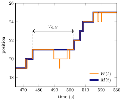
The alternative characterization of the fluctuations of the cycle starts from the winding number. In order to track forward progress only, we consider the maximal winding number so far,

$$M\!\left(t\right)\equiv\max_{t^{\prime}\leq t}\left\{W\!\left(t^{\prime}\right)\right\}.$$ (13)

For a molecular motor, the maximal winding number represents the furthest physical location reached yet. Because it can only increase, and subsequent values are independent and identically distributed, $M\!\left(t\right)$ is a renewal process [2]. As shown in Fig. 2, intervals of constant $M$ end whenever the winding number reaches a value that was not attained before. The stochastic waiting time of $M\!\left(t\right)$, defined as the time between two increments, is precisely $T_{N}$, because a first passage at the next cycle ends the period and raises the maximum winding number. Accordingly, $M\!\left(t\right)$ also counts the number of completed periods so far.

We may then define a randomness based on the maximal winding number as

$$r_{M}=\lim_{t\to\infty}\frac{\mathrm{Var}\!\left(M\!\left(t\right)\right)}{\langle M\!\left(t\right)\rangle}.$$ (14)

In the special case of irreversible cycles, $r_{M}$ as defined here reduces to the previous winding number randomness $r_{W}$ Eq. 2, since then $M\to W$. For general reversible cycles, $r_{W}$ and $r_{M}$ are not a priori equal.

Figure 2: Example time traces of the current cycle number of the particle (winding number $W\!\left(t\right)$), and the furthest position so far (maximum $M\!\left(t\right)$). The data are produced by kinetic Monte Carlo simulations of a system with $N=5$ states per cycle, and uniform rates, such that on average one forward substep is made per $1.0\text{\,}\mathrm{s}$, and one backward substep per $1.5\text{\,}\mathrm{s}$. As indicated in the main text, the stochastic period $T_{N}$ corresponds to the interval between two increments of $M\!\left(t\right)$, and has an average of $15\text{\,}\mathrm{s}$ in this example.

III Results

III.1 Equivalence of randomness parameters

Schnitzer and Block showed that $r_{W}$ and $r_{T}$ coincide for irreversible cycles, Eq. 3 [5]. It turns out that their proof carries over unchanged to the reversible system, when using the maximal winding number instead of the winding number. That is,

$$r_{T}=r_{M}.$$ (15)

The original proof of this relation was given by Smith [2] in the context of general renewal processes. It holds because $M\!\left(t\right)$ is a renewal process with waiting times $\sim T_{N}$, as indicated before. In the following, we will show that in fact not only Eq. 15 but also Eq. 3 holds for reversible cycles.

To that end, we first need to prove the following relation,

$$\lim_{t\rightarrow\infty}\frac{\mathrm{Var}\!\left(W\!\left(t\right)\right)}{\langle W\!\left(t\right)\rangle}=\lim_{t\rightarrow\infty}\frac{\mathrm{Var}\!\left(M\!\left(t\right)\right)}{\langle M\!\left(t\right)\rangle}.$$ (16)

It is convenient to study the nonpositive difference $\Delta\!\left(t\right)\equiv W\!\left(t\right)-M\!\left(t\right)$, which we use to rewrite

$$r_{W} =\lim_{t\rightarrow\infty}\!\frac{\mathrm{Var}\!\left[W\!\left(t\right)\right]}{\langle W\!\left(t\right)\rangle}$$

$$=\lim_{t\rightarrow\infty}\!\frac{\mathrm{Var}\!\left[M\!\left(t\right)\right]+\mathrm{Var}\!\left[\Delta\!\left(t\right)\right]+2\mathrm{Cov}\!\left[M\!\left(t\right),\Delta\!\left(t\right)\right]}{\langle M\!\left(t\right)\rangle+\langle\Delta\!\left(t\right)\rangle}.$$ (17)

Both the mean and variance of $M\!\left(t\right)$ grow linearly with $t$ in leading order [2]. We will show below that the mean and variance of $\Delta\!\left(t\right)$ stay finite for long times, implying that they do not contribute to the limit, Eq. 17. The remaining covariance term has bounds set by the Cauchy-Schwarz inequality [14],

$$\lvert\mathrm{Cov}\!\left[M\!\left(t\right),\Delta\!\left(t\right)\right]\rvert\leq\sqrt{\mathrm{Var}\!\left[M\!\left(t\right)\right]\mathrm{Var}\!\left[\Delta\!\left(t\right)\right]}.$$ (18)

If the variance of $\Delta\!\left(t\right)$ remains finite, then the covariance term in Eq. 17 grows slower than the leading term $\mathrm{Var}\!\left[M\!\left(t\right)\right]$, and will not contribute to the limit either. Then indeed Eq. 15 follows.

Hence, it remains to show that the first two statistical moments of $\Delta\!\left(t\right)$ actually stay finite in the long time limit. To this end we introduce the new microscopic variable $V\!\left(t\right)$, defined as

$$V\!\left(t\right)=Z\!\left(t\right)-NM\!\left(t\right).$$ (19)

$V\!\left(t\right)<N$ is the current offset from the furthest cycle reached. Our motivation for studying $V\!\left(t\right)$ is its relation to $\Delta\!\left(t\right)$,

$$\left\lfloor\frac{V\!\left(t\right)}{N}\right\rfloor =\left\lfloor\frac{Z\!\left(t\right)}{N}\right\rfloor-M\!\left(t\right)$$

$$=W\!\left(t\right)-M\!\left(t\right)$$

$$=\Delta\!\left(t\right).$$ (20)

Since $M\!\left(t\right)$ is derived from $Z\!\left(t\right)$, the new variable $V\!\left(t\right)$ is completely determined by $Z\!\left(t\right)$. In fact, by itself $V\!\left(t\right)$ constitutes a Markov chain, with a state transition diagram as shown in Fig. 1c. As shown there, one transition of this chain is irreversible.

To understand the one-way transition, we notice that the maximum winding number increases irreversibly from $M$ to $M+1$ whenever $Z\!\left(t\right)$ transitions from state $\left(M+1\right)N-1$ to state $\left(M+1\right)N$. Concurrently, $V\!\left(t\right)$ transitions from state $N-1$ to state $0$ (Eq. 19), effectively resetting it to the origin. Therefore, the irreversibility of the transition originates from that of $M\!\left(t\right)$.

Using the new Markov chain, we can show that the mean and variance of $V\!\left(t\right)$ and $\Delta\!\left(t\right)$ will tend to finite values. In contrast to $Z\!\left(t\right)$ on the integer line, which increases endlessly and thus has no stationary distribution, $V\!\left(t\right)$ does have a stationary distribution. As shown in detail in Sec. S.IV [12], the stationary probability distribution decreases exponentially for $V\!\left(t\right)\to-\infty$. Then, Eq. 20 implies that $\Delta\!\left(t\right)$ also has a stationary distribution with an exponential tail on the left. In other words, it is exponentially unlikely for the particle to move backwards a certain distance from the furthest point reached before. Because the stationary distribution of $\Delta\!\left(t\right)$ is bounded on the right and has an exponential tail on the left, it has finite moments of any order. In particular, this implies that as $t\to\infty$, the mean and variance of $\Delta\!\left(t\right)$ are $\mathcal{O}\left(t^{0}\right)$, so that the covariance term in Eq. 17 is $\mathcal{O}\left(t^{1/2}\right)$. This completes the proof of Eq. 16, and consequently establishes relation Eq. 15, so that in conclusion, we arrive at Eq. 3,

$$r\equiv r_{T}=r_{M}=r_{W}$$ (21)

for general reversible or irreversible reaction cycles.

III.2 Statistical moments of the period

The randomness parameter is useful for comparing experimental results to theoretical predictions. Chemla et al. derived the exact solution $r_{W}$ for reversible cycles [7], and this exact solution now carries over to $r_{T}$. Additionally, their analytical expression provides an alternative route for showing the equivalence of both forms of the randomness parameter. In this section we give analytical solutions of the moments of the first passage time, which directly give $r_{T}$. Comparing this result with that for $r_{W}$, we confirm the equivalence Eq. 21.

To find the moments of $T_{N}$, it is convenient to decompose the first passage time into first passage times at each microscopic interval,

$$T_{N}\sim T_{0,N}=\sum_{i=0}^{N-1}T_{i,i+1}.$$ (22)

Notice that a path causing a first passage is allowed to recross the initial point an arbitrary number of times before reaching the final point. We denote the first-passage time density of $T_{i,j}$ by $f_{i,j}\!\left(t\right)$. $S_{i}\!\left(t\right)$ denotes the survival probability at state $i$, given by $S_{i}(t)=\exp(-(k_{i+}+k_{i-})t)$. The single step first passage time distributions are linked by the relation

$$f_{i,i+1}\!\left(t\right)=S_{i}\!\left(t\right)k_{i+}\!+\!\int_{0}^{t}\!\mathop{}\!\mathrm{d}t^{\prime}S_{i}\left(t^{\prime}\right)k_{i-}f_{i-1,i+1}\!\left(t-t^{\prime}\right).$$ (23)

Eq. 23 splits the paths from $i$ to $i+1$ into paths where the first step is made in either the positive or negative direction. By taking the Laplace transform and using it as the moment generating function, we find relations for all statistical moments of $T_{i,i+1}$. In Sec. S.V [12], these coupled equations are derived and solved, providing exact solutions to the mean and variance of the stochastic period,

$$\langle T_{N}\rangle =\left(1-Q\right)^{-1}\sum_{i,j=0}^{N-1}\frac{1}{k_{i+}}\prod_{\ell=1}^{j}\frac{k_{\left(i+\ell\right)-}}{k_{\left(i+\ell\right)+}};$$

$$\mathrm{Var}\!\left(T_{N}\right) =\left(1-Q\right)^{-3}\sum_{i=0}^{N-1}\left[\sum_{j=0}^{N-1}\frac{1}{k_{\left(i-j\right)+}}\prod_{\ell=1}^{j}\frac{k_{\left(i-j+\ell\right)-}}{k_{\left(i-j+\ell\right)+}}\right]^{2}$$

$$\qquad\times\left(1+2\sum_{j=1}^{N-1}\prod_{\ell=1}^{j}\frac{k_{\left(i+\ell\right)-}}{k_{\left(i+\ell\right)+}}+\prod_{\ell=0}^{N-1}\frac{k_{\ell-}}{k_{\ell+}}\right).$$ (24)

Here, $Q$ is the product of the rates as in Eq. 5.

We inserted the analytical moments Eq. 24 in Eq. 12 to obtain an exact expression for $r_{T}$. We then compared this to the analytical expression for $r_{W}$ obtained by Chemla et al. [7]. While Eq. 21 implies that they must be identical, we were unable to rewrite our analytical expression in the form of that of Chemla et al. due to the complexity of the expressions. Still, using the computer algebra system Mathematica [15], we have directly confirmed their equivalence up to $N=55$, suggesting it holds for arbitrary $N$ (as Eq. 21 implies), and lending strong support for Eq. 24 and the result by Chemla et al.

III.3 Optimal precision of the period

Figure 3: Dissipation suppresses fluctuations. The randomness parameter is calculated in the optimal case of uniform rates, as a function of the number of steps per cycle $N$ and the dissipation per cycle $\Delta F$. It is evident that for low dissipation, increasing the number of steps cannot lower the randomness parameter. However, when the free energy drop per cycle becomes large ($\Delta F\geq 2Nk_{B}T$), $N$ becomes limiting and the precision increases only with increasing the number of substeps. The dotted lines represent the final inequality in Eq. 25 for the case $N=5$.

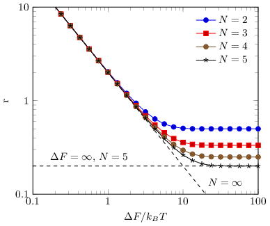
In recent work, Barato and Seifert introduced a so-called thermodynamic uncertainty relation, which bounds the minimum value of the Fano factor $r_{W}$ in the long time limit [8] in terms of the number of substates and the energy dissipation rate. The bound was subsequently proved by Gingrich et al. [16]. Combined with our result Eq. 21, the bound reads

$$r_{T} =r_{W}$$

$$\geq\frac{1}{N}\coth\left(\frac{\Delta F}{2Nk_{B}T}\right)$$

$$\geq\max\left\{\frac{2k_{B}T}{\Delta F},\frac{1}{N}\right\}.$$ (25)

The first inequality is the thermodynamic uncertainty relation [8, 16]; it is saturated for a cycle with uniform forward and backward rates, such that $k_{i\pm}=k_{\pm}$. The second, looser inequalities are found in the limit that either $N$ or $\Delta F$ approaches infinity. Hence, the equivalence of the different randomness parameters Eq. 21 extends the uncertainty relation to the cycle period, which therefore has direct implications for the workings of molecular clocks.

The bound Eq. 25 for the precision of timing $r_{T}$ constrains the optimal design of biochemical timekeeping mechanisms. Circadian clocks are present in many organisms, such as the relatively simple cyanobacteria [17]. Here, a post-translational modification cycle produces approximately $24$ hour rhythms [18]. Although in real cyanobacteria many KaiABC protein complexes in a bacterium go through their biochemical modification cycles in a partly synchronized way, we can expect that the single-cycle expression Eq. 25 gives a correct intuition about the limiting resources: A precise clock period requires both a sufficient number of cyclic substates and an adequate cycle affinity. When both the average period of the cycle and the free energy dissipation per cycle are held constant, then the lowest possible variance is achieved by choosing uniform rates [8, 16]. Furthermore, to prevent wasting resources, it is beneficial to tune both the number of steps $N$ and the free energy dissipation, such that both bounds on the final line of Eq. 25 are equally limiting,

$$N_{\mathrm{opt}}=\frac{\Delta F_{\mathrm{opt}}}{2k_{B}T}.$$ (26)

Fig. 3 shows that when $\Delta F/k_{B}T$ is small, it limits the precision, meaning that the optimal randomness is independent of $N$. In other words, the low free energy investment cannot be compensated by a large number of substeps. Conversely, when $\Delta F/k_{B}T$ is larger than $2N$, it has hardly any benefit in reducing the randomness. The number of substeps then limits the precision, and the latter can only increase by increasing $N$. A similar design principle has recently been obtained for the optimal allocation of resources in cellular sensing [19, 20]. In an optimally designed system, each fundamental resource should be equally limiting.

III.4 Measurement protocols

The two equivalent forms $r_{T}=r_{W}$ of the randomness parameter relate to two alternative methods of measuring the stochasticity of an enzymatic cycle [5]. A prolonged measurement of the time trace of a single motor protein position may include many ($M$) completed periods, giving $M$ samples for computing the randomness parameter $r_{T}$ (see Fig. 2). However, as pointed out by Schnitzer and Block [5], experimental measurements of each period may require a high temporal and spatial resolution. In the example of a motor protein, it would be essential to track the timing and direction of each physical step. When such measurement precision is not available, $r_{W}$ gives another option for measuring the randomness, since it only requires samples of the number of completed cycles $W\!\left(t\right)$. For a motor, this corresponds to the final distance traveled after a certain time, while for enzymatic cycles it coincides with the number of product molecules. Multiple independent samples are needed in order to measure $r_{W}$ via Eq. 2. This data can either be gained from a collection of propagating molecules, or from sections of a single long time trace. This way, when the resolution to measure individual periods and to estimate $r_{T}$ is missing, $r_{W}$ can still provide an estimate for the randomness parameter.

Now, considering the case where the measurement precision is sufficient for determining either $r_{T}$ or $r_{W}$, is there one that converges quicker to the desired result? In Sec. S.VI [12] we compare the estimation of $r_{W}$ and $r_{T}$ from similar sets of data, to investigate the differences between their estimation errors. We use a simple method to calculate both versions of the randomness parameter, and show that estimation of $r_{W}$ involves a trade-off in the finite observation time $t$ after which samples of $W\!\left(t\right)$ are taken. For short $t$, many samples of $W\!\left(t\right)$ are found, but the result suffers from a significant systematic bias. For large $t$, the bias disappears since we approach the limit in definition Eq. 2, but the number of samples decreases, reducing the precision. The estimate of $r_{T}$ is not subject to this trade-off, and appears to converge quicker than that of $r_{W}$, because $T_{N}$ can be sampled more frequently than $W\!\left(t\right)$. Therefore, $r_{T}$ should be favored when the experimental resolution allows it; use of $r_{W}$ requires careful correction of the finite-time bias.

IV Discussion

In recent works, efforts were made to study temporal precision in stochastic networks. Barato and Seifert considered either the Fano factor $r_{W}$ [21, 22], or the coherence time of oscillations in the occupancy of a single site [23]. Here we have presented the equivalence Eq. 21 for reversible cycles, showing that the Fano factor $r_{W}$ can be reinterpreted as a clock precision by relating it to the fluctuations in the period $r_{T}$. This in turn widens the applicability of the thermodynamic uncertainty relation [8] to temporal variables. In the example of molecular clocks, it translates to a bound for the clock precision of reversible cycles. A cycle reaches the highest timing accuracy when all transitions have uniform forward- and backward rates. As intuitively expected, the bound shows that the period can become more deterministic when either the number of substates per cycle or the free energy dissipation per cycle is increased. Yet both these quantities are fundamentally limiting the precision, meaning that each sets its own lower bound on the precision, and that one cannot compensate for the other [19, 20].

The second study [23] employs a different approach to quantifying the precision of biochemical clocks, which can be applied to any non-equilibrium network, and involves defining an average period as a property of the transition matrix. That average period is not to be confused with the stochastic period $T_{N}$ defined here, which is a random variable; their relation in the case of cyclic networks is an interesting open question.

In a different work, Barato and Seifert discuss the information contained in higher moments of the period and propose bounds on the skewness and kurtosis for irreversible cycles [24]. We show how to calculate these moments for reversible cycles in section III.2. It would be interesting to see whether tighter lower bounds exist for the higher moments just as for the randomness parameter, and whether those bounds are saturated for a system with uniform rates.

Very recently, Gingrich and Horowitz reported a relation between the large deviation functions for currents and first passage times in general Markov chains [25], which applies to the present setup. They also made a connection between the thermodynamic uncertainty relation and first passage time statistics. The main contribution of our present work is a proof of the identification $r_{T}=r_{W}$, Eq. 21 for unicyclic networks. Using the concept of a stochastic period, our direct derivation of this equivalence also affords physical intuition for the relation of current and first-passage time in cycles.

It is intriguing to ask if the equivalence Eq. 21 holds for more general network topologies than the reversible cycle as shown in Fig. 1a. Indeed, by examining the derivations one can see that Eq. 21 holds in more general networks if they fulfill the following conditions. First, it must be possible to define a winding number $W\!\left(t\right)$, of which the average has a forward drift. This condition is already fulfilled by taking $W\!\left(t\right)$ as the net number of times a specific transition in the network is made, whenever there is a stationary net forward flux through this pathway. The renewal process $M\!\left(t\right)$ derived from the winding number then obeys Eq. 15, where the period is defined as the waiting time of the renewal process. Second, the difference $\Delta\!\left(t\right)$ between the current- and maximum position should have a limiting distribution with a finite average and variance. This condition ensures that Eq. 16 holds. It remains to be seen which networks conform to these conditions, and whether the first condition implies the second.

Supplemental Material:
Quantifying fluctuations in reversible enzymatic cycles and clocks

S.I Proof that the particle moves forward

The cyclic Markov chain $C\!\left(t\right)$ and its unwound version $Z\!\left(t\right)$, as defined in Eq. 4 and Eq. 6 of the main text respectively, have several interesting properties. In this section, we will show that the non-equilibrium driving of the cycle, which is set by the exponentiated affinity $Q<1$, logically implies that a particle will make an arbitrary number of forward transitions with probability $1$. This fact is used for the definition of the period in Sec. II of the main text.

As mentioned in the main text, $T_{i,j}$ is the first passage time at state $j$ given that the particle started in state $i$, and $f_{i,j}\!\left(t\right)$ is its probability density function. We denominate the probability that a particle will make at least one passage at $j$ by $\alpha_{i,j}$. This fraction is given by the integral of the first passage time density over all time, and thus the goal of this section is to show that

$$\alpha_{i,j}\equiv\int_{0}^{\infty}\!\mathop{}\!\mathrm{d}tf_{i,j}\!\left(t\right)=1\qquad\mathrm{if}\;i<j\;\mathrm{and}\;Q<1.$$ (S.1)

Before we arrive at this result, we describe some of the characteristics of the Markov chain $Z\!\left(t\right)\in\mathbb{Z}$.

First, we would like to find relations for the first passage time distributions $f_{i,j}\!\left(t\right)$, with $i<j$. For this, it is helpful to define the survival probability at a specific point as

$$S_{i}\!\left(t\right)=e^{-\left(k_{i+}+k_{i-}\right)t}.$$ (S.2)

The survival probability is defined as the probability that a particle remains at location $i$ for at least a time $t$, meaning that it has not transitioned yet. When this probability is multiplied with the rate of making transitions, one finds the probability density of waiting times at state $i$. The first step, which ends such a waiting time, can either be in the forward or in the backward direction. Accordingly, the first passage time density from $i$ to $j$ can be conditioned on the direction of this first step. If the step moves the particle from $i$ to $i\pm 1$ at exactly time $t^{\prime}$, then the particle still needs to travel from state $i\pm 1$ to $j$ in precisely the remaining time $t-t^{\prime}$, in order to complete the first passage. This provides the following fundamental relation on the single step first passage times,

$$f_{i,j}\!\left(t\right)=\int_{0}^{t}\mathop{}\!\mathrm{d}t^{\prime}\left[S_{i}\!\left(t^{\prime}\right)k_{i+}f_{i+1,j}\!\left(t-t^{\prime}\right)+S_{i}\!\left(t^{\prime}\right)k_{i-}f_{i-1,j}\!\left(t-t^{\prime}\right)\right].$$ (S.3)

For $i=j-1$ the equation changes, because a single forward step creates a first passage directly,

$$f_{j-1,j}\!\left(t\right)=S_{j-1}\!\left(t\right)k_{j-1+}+\int_{0}^{t}\mathop{}\!\mathrm{d}t^{\prime}S_{j-1}\!\left(t^{\prime}\right)k_{j-1-}f_{j-2,j}\!\left(t-t^{\prime}\right).$$ (S.4)

These equations can be used to show that the particle will always move forward. The following proof of Eq. S.1 resembles that given by e.g. Anderson [1].

A condition for the $\alpha_{i,j}$ is found by integrating both sides of Eq. S.3 over all $t\geq 0$. This integral turns the convolutions into simple products of the separate integrals, and the integral of Eq. S.2 can be easily computed, leading to

$$\alpha_{i,j}=\frac{k_{i+}}{k_{i+}+k_{i-}}\alpha_{i+1,j}+\frac{k_{i-}}{k_{i+}+k_{i-}}\alpha_{i-1,j},$$ (S.5)

whereas for $i=j-1$, we find

$$\alpha_{j-1,j}=\frac{k_{j-1+}}{k_{j-1+}+k_{j-1-}}+\frac{k_{j-1-}}{k_{j-1+}+k_{j-1-}}\alpha_{j-2,j}.$$ (S.6)

The denominators of Eq. S.5 and Eq. S.6 can be brought to their respective left hand sides, revealing that

$$\left(\alpha_{i,j}-\alpha_{i-1,j}\right) =\frac{k_{i+}}{k_{i-}}\left(\alpha_{i+1,j}-\alpha_{i,j}\right)\qquad\mathrm{if}\>i<j-1$$

$$\left(\alpha_{j-1,j}-\alpha_{j-2,j}\right) =\frac{k_{j-1+}}{k_{j-1-}}\left(1-\alpha_{j-1,j}\right).$$ (S.7)

Recursive use of this equation gives

$$\left(\alpha_{i,j}-\alpha_{i-1,j}\right)=\left(1-\alpha_{j-1,j}\right)\prod_{\ell=i}^{j-1}\frac{k_{\ell+}}{k_{\ell-}}.$$ (S.8)

This allows us to express each probability in terms of $\alpha_{j-1,j}$,

$$\alpha_{i,j} =\alpha_{j-1,j}+\sum_{h=i+1}^{j-1}\left(\alpha_{h-1,j}-\alpha_{h,j}\right)$$

$$=\alpha_{j-1,j}-\left(1-\alpha_{j-1,j}\right)\sum_{h=i+1}^{j-1}\prod_{\ell=h}^{j-1}\frac{k_{\ell+}}{k_{\ell-}},$$ (S.9)

where we have to remember that we are only considering the case that $i<j$. The formula can be checked for $i=j-1$, in which case the summation from $j$ to $j-1$ vanishes by definition of the sum, and only the first term survives.

Next, it is possible to take the limit of $i\rightarrow-\infty$. Furthermore, notice that

$$\sum_{h=-\infty}^{j-1}x_{h}=\sum_{m=-\infty}^{0}\sum_{n=j-N}^{j-1}x_{mN+n}$$ (S.10)

for any $x_{h}$, and

$$\prod_{\ell=mN+n}^{j-1}x_{\ell}=\left(\prod_{\ell=mN+n}^{n-1}x_{\ell}\right)\left(\prod_{\ell=n}^{j-1}x_{\ell}\right)=\left(\prod_{\ell=mN}^{-1}x_{\ell}\right)\left(\prod_{\ell=n}^{j-1}x_{\ell}\right),$$ (S.11)

where the last equality is true when $x_{h+mN}=x_{h}$. This step becomes clear by rearranging the front and the back of the product to make it independent of $n$. Eq. S.10 and Eq. S.11 imply that

$$\lim_{i\rightarrow-\infty}\alpha_{i,j} =\alpha_{j-1,j}-\left(1-\alpha_{j-1,j}\right)\sum_{m=-\infty}^{0}\sum_{n=j-N}^{j-1}\prod_{\ell=mN+n}^{j-1}\frac{k_{\ell+}}{k_{\ell-}}$$

$$=\alpha_{j-1,j}-\left(1-\alpha_{j-1,j}\right)\Bigg[\sum_{n=j-N}^{j-1}\prod_{\ell=n}^{j-1}\frac{k_{\ell+}}{k_{\ell-}}\Bigg]\Bigg[\sum_{m=-\infty}^{0}\prod_{\ell=mN}^{-1}\frac{k_{\ell+}}{k_{\ell-}}\Bigg]$$

$$=\alpha_{j-1,j}-\left(1-\alpha_{j-1,j}\right)\Bigg[\sum_{n=j-N}^{j-1}\prod_{\ell=n}^{j-1}\frac{k_{\ell+}}{k_{\ell-}}\Bigg]\sum_{m=0}^{\infty}\left(Q^{-1}\right)^{m}.$$ (S.12)

In the final step, we used the definition of $Q$ from Eq. 5 of the main text to rewrite the product over $N$ subsequent fractions of rates. Additionally, the cyclic symmetry of the rates $k_{mN+l\pm}=k_{l\pm}$ was applied to see that $Q$ emerges at each interval. The final sum of Eq. S.12 diverges, since we made the choice $Q<1$. However, the limit of $\alpha_{i,j}$ must be a number between $0$ and $1$, because it represents a probability. The only way this is possible is when $\alpha_{j-1,j}=1$, because this takes out the diverging term before the limit is taken. Now the proof is easily finalized, as Eq. S.9 shows that

$$\alpha_{i,j}=1\qquad\forall\>i<j.$$ (S.13)

S.II Period invariance under translations

To ensure a proper definition of the period in Sec. II of the main text, it is important that the cycle completion time is not influenced by the initial position. If a different period existed for each initial state, this would disagree with the intuition that oscillations are a property of the system as a whole. In the following, we show that the stochastic time interval $T_{0,N}$ complies with this requirement.

Firstly, the transition rates in the system are symmetric under translations by multiples of $N$, causing the statistics of the first passage times to obtain an identical symmetry,

$$T_{i+mN,j+mN}\sim T_{i,j}\qquad\forall m\in\mathbb{Z}.$$ (S.14)

Here, $\sim$ means that both variables are identically distributed. Focusing on $T_{0,N}$, a first passage at $N>1$ requires passages at all intermediate points. Hence, the stochastic period can be decomposed into the first passage times between all unique forward transitions,

$$T_{0,N}=\sum_{i=0}^{N-1}T_{i,i+1}.$$ (S.15)

Furthermore, the strong Markov property implies that all intermediate first passage times are statistically independent, showing that we can solve the distribution of the full period by calculating the distributions of the intermediate intervals. This will be important in Sec. S.V, where we calculate the statistical moments of the period.

To show that the period is independent from the initial state, the general initial position is taken to be any $j\in\mathbb{Z}$. Eq. S.14 implies that this initial position can be chosen such that $0\leq j\leq N-1$ without influencing the distribution. Then, the first passage time is decomposed as in Eq. S.15,

$$T_{j,j+N} =\sum_{i=j}^{j+N-1}T_{i,i+1}$$

$$=\sum_{i=j}^{N-1}T_{i,i+1}+\sum_{i=N}^{j+N-1}T_{i,i+1}$$

$$\sim\sum_{i=j}^{N-1}T_{i,i+1}+\sum_{i=0}^{j-1}T_{i,i+1}$$

$$=\sum_{i=0}^{N-1}T_{i,i+1}=T_{0,N}.$$ (S.16)

In this notation, a summation from $0$ to $-1$ vanishes. In going from the second to the third line, Eq. S.14 is used to lower the index by $N$. As a result, it is shown that the initial position $j$ has no influence on the time it takes to complete a net full cycle. Hence, the period in unambiguously defined, and it is justified to call it $T_{N}\equiv T_{0,N}\sim T_{j,j+N}$, without indicating the initial position.

S.III Connection between flux and average period

The average period $\langle T_{0,N}\rangle$ can be related to the steady state flux of the cycle $C\!\left(t\right)$. To show this connection, we follow a strategy that is similar to the one showing the equivalence between $r_{T}$ and $r_{W}$ in the main text. Since the maximum winding number $M\!\left(t\right)$ is a renewal process, we can apply the elementary renewal theorem, which states [2]

$$\lim_{t\rightarrow\infty}\frac{\langle M\!\left(t\right)\rangle}{t}=\lim_{t\rightarrow\infty}\frac{d\langle M\!\left(t\right)\rangle}{dt}=\frac{1}{\langle T_{0,N}\rangle}.$$ (S.17)

The first step is due to l’Hôpital’s rule. A connection can be made with the current winding number $W\!\left(t\right)$, using the definition of $\Delta\!\left(t\right)$,

$$\lim_{t\rightarrow\infty}\frac{d\langle W\!\left(t\right)\rangle}{dt}=\lim_{t\rightarrow\infty}\frac{\langle W\!\left(t\right)\rangle}{t}=\lim_{t\rightarrow\infty}\frac{\langle M\!\left(t\right)\rangle+\langle\Delta\!\left(t\right)\rangle}{t}=\lim_{t\rightarrow\infty}\frac{\langle M\!\left(t\right)\rangle}{t},$$ (S.18)

which uses the fact that the average of $\Delta\!\left(t\right)$ becomes constant in steady state, as shown in Sec. S.IV, while the average of $M\!\left(t\right)$ increases linearly with time in leading order. The latter follows from the elementary renewal theorem, see e.g. Smith [2]. The left hand side of the equation can be expressed in terms of $Z\!\left(t\right)$ and its probability distribution $p_{i}\!\left(t\right)\equiv\mathbb{P}\left\{Z\!\left(t\right)=i\right\}$,

$$\frac{d\langle W\!\left(t\right)\rangle}{dt} =\frac{d}{dt}\sum_{m=-\infty}^{\infty}m\sum_{i=0}^{N-1}p_{mN+i}\!\left(t\right)$$

$$=\sum_{m=-\infty}^{\infty}m\sum_{i=0}^{N-1}\left[-\left(k_{i+}+k_{i-}\right)p_{mN+i}\!\left(t\right)+k_{i-1+}p_{mN+i-1}\!\left(t\right)+k_{i+1-}p_{mN+i+1}\!\left(t\right)\right]$$

$$=\sum_{m=-\infty}^{\infty}m\left[-k_{N-1+}p_{\left(m+1\right)N-1}\!\left(t\right)-k_{0-}p_{mN}\!\left(t\right)+k_{N-1+}p_{mN-1}\!\left(t\right)+k_{0-}p_{\left(m+1\right)N}\!\left(t\right)\right]$$

$$=\sum_{m=-\infty}^{\infty}\left[m-\left(m-1\right)\right]\left[k_{N-1+}p_{mN-1}\!\left(t\right)-k_{0-}p_{mN}\!\left(t\right)\right]$$

$$=k_{N-1+}\sum_{m=-\infty}^{\infty}p_{mN-1}\!\left(t\right)-k_{0-}\sum_{m=-\infty}^{\infty}p_{mN}\!\left(t\right).$$ (S.19)

In the second line, we use the transition matrix from Eq. 6 of the main text to evaluate the time derivative. Then, the terms in the sum over $i$ that cancel each other are taken out. Finally, we relabel $m$ to $m-1$ in the terms where the factor $m+1$ is present in the label, such that the final result emerges. The two sums over probabilities can be reinterpreted in connection with the Markov process on the circular state space. Eq. 8 of the main text implies that the probability that $C\!\left(t\right)$ equals $i$ can be expanded as a sum over the possible values of $Z\!\left(t\right)$,

$$\mathrm{P}\left\{C\!\left(t\right)=i\right\}=\sum_{m=-\infty}^{\infty}p_{mN+i}\!\left(t\right).$$ (S.20)

Since $C\!\left(t\right)$ has a finite state space, it has a limiting distribution, which we call $\pi_{i}$. Combining all previous equations, and taking the long time limit, we find a connection between the steady state flux through the cycle $J$, and the average first passage time,

$$\frac{1}{\langle T_{0,N}\rangle}=k_{N-1+}\pi_{N-1}-k_{0-}\pi_{0}=J.$$ (S.21)

We make use of this fact in Sec. II of the main text. Notice that $J$ is constant through the cycle by definition of the steady state, i.e.

$$J=k_{i+}\pi_{i}-k_{i+1-}\pi_{i+1}\quad\forall i.$$ (S.22)

Combined with Eq. S.21, this also implies Eq. S.16. Hence, we may redefine the cycle start point arbitrarily.

S.IV Stationary distribution of $V\!\left(t\right)$

In this section, we show that the Markov process $V\!\left(t\right)$, which is shown in Fig. 1 of the main text, has a stationary distribution. Furthermore, the exact form of the stationary probability will be derived, showing that it has an exponentially decaying tail. The latter property will be used to show that the moments of $\Delta\!\left(t\right)$ will remain constant in the long time limit, which is an important step in Sec. III A of the main text.

First, we need to show that the stationary distribution exists. For this, we use the definition of the steady state flux

$$J_{i}\equiv k_{i+}\phi_{i}-k_{i+1-}\phi_{i+1}$$ (S.23)

for $i<N-1$, where $\phi_{i}$ is the sought after stationary distribution of $V\!\left(t\right)$. Additionally, a special definition is used for the only irreversible step of the chain,

$$J_{N-1}\equiv k_{N-1+}\phi_{N-1}.$$ (S.24)

The stationary distribution is the solution of the following set of equations,

$$J_{i}-J_{i-1}=0\qquad \mathrm{for}\quad i<0$$

$$J_{0}-J_{-1}-J_{N-1}=0\qquad \mathrm{for}\quad i=0$$

$$J_{i}-J_{i-1}=0\qquad \mathrm{for}\quad 0<i\leq N-1$$

$$\sum_{i=-\infty}^{N-1}\phi_{i}=1.\qquad$$ (S.25)

The fist equation shows that

$$J_{i-1}=J_{i}=J_{-1}\qquad\forall i<0.$$ (S.26)

The second equality follows from applying an inductive step to the first equality. Hence, the flux in the infinite chain is constant. Additionally, the stationary distribution only exists if the final normalization condition of Eq. S.25 is obeyed. For this, it is required that the stationary distribution vanishes infinitely far away,

$$\lim_{i\rightarrow-\infty}\phi_{i}=0.$$ (S.27)

Together with Eq. S.23 and Eq. S.26, it implies that

$$J_{i}=0\qquad\forall i<0.$$ (S.28)

Thus, if the stationary distribution exists, then detailed balance is obeyed on the negative integer tail. In this case, the flux equations in Eq. S.25 reduce to those of a cycle without the integer tail,

$$J_{0}-J_{N-1}=0\qquad \mathrm{for}\quad i=0$$

$$J_{i}-J_{i-1}=0\qquad \mathrm{for}\quad 0<i\leq N-1.$$ (S.29)

Consequently, the part of the solution for $i\geq 0$ is proportional to the stationary probability of a cycle with an equal transition matrix. Previously, exact solutions of this stationary distribution were reported for arbitrary rates, which were derived using various methods [3, 4]. Therefore, by inserting the rates including the irreversible step, Eq. S.29 can be solved in terms of $\phi_{0}$. In addition, Eq. S.28 for the tail probabilities has a simple solution in terms of $\phi_{0}$,

$$\phi_{i}=\phi_{0}\prod_{\ell=i}^{-1}\frac{k_{\ell+1-}}{k_{\ell+}},$$ (S.30)

which holds for $i\leq 0$. Both solutions, for the circle and the tail, are connected at $\phi_{0}$. We can combine them by normalization, to obtain the full solution of Eq. S.25,

$$\phi_{i}=\begin{cases}\frac{1}{\mathcal{N}_{\phi}}\left(\sum_{j=0}^{N-1}\prod_{\ell=1}^{j}\frac{k_{\ell-}}{k_{\ell+}}\right)\prod_{m=0}^{-\left(i+1\right)}\frac{k_{-m-}}{k_{-\left(m+1\right)+}}\text{ for }i\leq 0\\ \frac{1}{\mathcal{N}_{\phi}}\frac{k_{0+}}{k_{i+}}\left(\sum_{j=0}^{N-i-1}\prod_{\ell=1}^{j}\frac{k_{i+\ell-}}{k_{i+\ell+}}\right)\text{ for }0\leq i\leq N-1.\end{cases}$$ (S.31)

Notice that the two definitions coincide for $i=0$. These equations solve all linear equations Eq. S.25, with as many variables as conditions, and thus provide a unique solution. However, it was assumed that a solution exists, and this is only true if the normalization constant converges,

$$\mathcal{N}_{\phi} =\sum_{i=1}^{N-1}\frac{k_{0+}}{k_{i+}}\left(\sum_{j=0}^{N-i-1}\prod_{\ell=1}^{j}\frac{k_{i+\ell-}}{k_{i+\ell+}}\right)$$

$$+\sum_{i=-\infty}^{0}\left(\sum_{j=0}^{N-1}\prod_{\ell=1}^{j}\frac{k_{\ell-}}{k_{\ell+}}\right)\prod_{m=0}^{-\left(i+1\right)}\frac{k_{-m-}}{k_{-\left(m+1\right)+}}.$$ (S.32)

The first sum has finite bounds, so it trivially converges. The second sum consists of a factor times the following series,

$$\sum_{i=-\infty}^{0}\prod_{m=0}^{-\left(i+1\right)}\frac{k_{-m-}}{k_{-\left(m+1\right)+}}$$

$$=\sum_{i=0}^{\infty}\prod_{m=0}^{i-1}\frac{k_{-m-}}{k_{-\left(m+1\right)+}}$$

$$=\sum_{j=0}^{\infty}\sum_{i=0}^{N-1}\prod_{m=0}^{i+jN-1}\frac{k_{-m-}}{k_{-\left(m+1\right)+}}$$

$$=\sum_{j=0}^{\infty}\sum_{i=0}^{N-1}\prod_{m=0}^{jN-1}\frac{k_{-m-}}{k_{-\left(m+1\right)+}}\prod_{n=jN}^{jN+i-1}\frac{k_{-n-}}{k_{-\left(n+1\right)+}}$$

$$=\left(\sum_{i=0}^{N-1}\prod_{n=0}^{i-1}\frac{k_{-n-}}{k_{-\left(n+1\right)+}}\right)\sum_{j=0}^{\infty}\prod_{m=0}^{jN-1}\frac{k_{-m-}}{k_{-\left(m+1\right)+}}$$

$$=\left(\sum_{i=0}^{N-1}\prod_{n=0}^{i-1}\frac{k_{-n-}}{k_{-\left(n+1\right)+}}\right)\sum_{j=0}^{\infty}Q^{j}.$$ (S.33)

On the third line, the sum over $i$ is decomposed into a sum over the cycles, and a sum within the cycle. Then, after splitting the product into two parts, the fifth line makes use of the periodic property of the rates, causing $k_{-n+jN\pm}=k_{-n\pm}$. On the final line, $Q$ is recognized in a slightly different form, again valid due to periodicity,

$$Q=\prod_{\ell=0}^{N-1}\frac{k_{\ell-}}{k_{\ell+}}=\prod_{m=0}^{N-1}\frac{k_{-m-}}{k_{-\left(m+1\right)+}}.$$ (S.34)

In the final form of Eq. S.33, the geometric series is uncovered. Since the choice $Q<1$ was made in the definition of the Markov process $Z\!\left(t\right)$, the series converges. Hence, a unique stationary distribution exists, and is given by Eq. S.31. Moreover, for negative $i$, it can be seen that the limiting probability decays exponentially with the distance from $i=0$,

$$\phi_{i-N}=Q\phi_{i}.$$ (S.35)

This provides the proof that the moments of the difference to the maximum remain finite. The probability distribution for $\Delta\!\left(t\right)$ can be expressed in terms of the probability distribution for $V\!\left(t\right)$,

$$\mathrm{P}\left\{\Delta\!\left(t\right)=-n\right\}=\sum_{i=0}^{N-1}\mathrm{P}\left\{V\!\left(t\right)=-nN+i\right\}$$ (S.36)

for $n\leq 0$. For large $t$, this probability will approach its stationary distribution, and Eq. S.35 guarantees that it decays exponentially too,

$$\mathrm{P}\left\{\Delta\left(\infty\right)=-n\right\}=Q^{n-1}\mathrm{P}\left\{\Delta\left(\infty\right)=-1\right\}.$$ (S.37)

Since all moments of any distribution with exponential tails are finite, and $V\!\left(t\right)$ reaches its stationary state in the infinite time limit, this completes the proof that the mean and variance of $\Delta\!\left(t\right)$ that occur in Eq. 17 of the main text will remain finite.

S.V Analytical solutions of the statistical moments of the period

For many applications, from mathematical proofs to numerical evaluation, it is helpful to have analytical expressions of key quantities. Here, we study the stochasticity of the period, which is generally quantified using the statistical moments of its distribution, and provide a method to calculate these moments. For example, the mean and variance of the period are derived, which are utilized in Sec. III B of the main text.

From Eq. S.15 and the statistical independence of the $T_{j,j+1}$, it follows that the mean and variance of $T_{0,N}$ can be split into those of the single step first passage times,

$$\langle T_{0,N}\rangle =\sum_{i=0}^{N-1}\langle T_{i,i+1}\rangle$$

$$\mathrm{Var}\left(T_{0,N}\right) =\sum_{i=0}^{N-1}\mathrm{Var}\left(T_{i,i+1}\right).$$ (S.38)

The decomposition of the random variable $T_{0,N}$ in Eq. S.15 is equivalent to separating the distribution $f_{0,N}\!\left(t\right)$ using an N-fold convolution,

$$f_{0,N}\!\left(t\right)=\int_{0}^{t}\prod_{i=0}^{N}\Bigg[\mathop{}\!\mathrm{d}t_{i}\,f_{i,i+1}\!\left(t_{i}\right)\Bigg]\delta\!\left(t-\sum_{i=0}^{N-1}t_{i}\right).$$ (S.39)

Here, $\delta\!\left(t\right)$ represents the Dirac delta function, and the product affects both the variables of integration and the single step first passage time densities. The Laplace transform of Eq. S.39 gives

$$\widetilde{f}_{0,N}\!\left(s\right)=\prod_{i=0}^{N-1}\widetilde{f}_{i,i+1}\!\left(s\right).$$ (S.40)

This equation will be useful for finding the closed form expressions for the statistical moments of $T_{0,N}$.

To start the derivation of the moments, we need a relation on the probability distribution of the period, for which we recall Eq. S.4,

$$f_{i,i+1}\!\left(t\right)=S_{i}\!\left(t\right)k_{i+}+\int_{0}^{t}\mathop{}\!\mathrm{d}t^{\prime}S_{i}\!\left(t^{\prime}\right)k_{i-}f_{i-1,i+1}\!\left(t-t^{\prime}\right).$$ (S.41)

To remove the convolution, we apply the Laplace transform to both sides of this relation. The final term can be decomposed using the same approach as in Eq. S.40,

$$\widetilde{f}_{i-1,i+1}\!\left(s\right)=\widetilde{f}_{i-1,i}\!\left(s\right)\widetilde{f}_{i,i+1}\!\left(s\right).$$ (S.42)

This produces a set of $N$ second order equations in $\widetilde{f}_{jj+1}\!\left(s\right)$,

$$\left(s+k_{i+}+k_{i-}\right)\widetilde{f}_{i,i+1}\!\left(s\right)=k_{i+}+k_{i-}\widetilde{f}_{i-1,i}\!\left(s\right)\widetilde{f}_{i,i+1}\!\left(s\right).$$ (S.43)

Since the equations are of second order, there will be two solutions. The appropriate solution can be chosen by realizing that the drift, set by $Q<1$, causes the particles to move forward. Sec. S.I shows that the choice $Q<1$ ensures that a first passage in the forward direction is made with probability 1, and thus $\widetilde{f}_{j,j+1}\!\left(0\right)=\alpha_{j,j+1}=1$. It becomes clear immediately by setting $s=0$ in Eq. S.43 that $\widetilde{f}_{j,j+1}\!\left(0\right)=1$ solves the equation at this specific point.

Moments of the first-passage time can be calculated by evaluating derivatives of the Laplace transformed distribution at $s=0$. Hence, relations for the moments are obtained by applying the derivative operator to Eq. S.43. For $n\geq 1$, the $n$th order derivative of Eq. S.43 gives the following relation,

$$\left(s+k_{i+}+k_{i-}\right)\widetilde{f}_{i,i+1}^{(n)}\!\left(s\right)+n\widetilde{f}_{i,i+1}^{(n-1)}\!\left(s\right)=k_{i-}\sum_{\ell=0}^{n}\binom{n}{\ell}\widetilde{f}_{i-1,i}^{(\ell)}\!\left(s\right)\widetilde{f}_{i,i+1}^{(n-\ell)}\!\left(s\right).$$ (S.44)

These equations become relevant by setting $s=0$, using the moment generating property of the Laplace transform and $\widetilde{f}_{j,j+1}\!\left(0\right)=1$. Upon a slight reorganisation, relations are uncovered for the moments of the single step first passage times,

$$k_{i+}\langle T_{i,i+1}^{n}\rangle-k_{i-}\langle T_{i-1,i}^{n}\rangle=n\langle T_{i,i+1}^{n-1}\rangle+k_{i-}\sum_{\ell=1}^{n-1}\binom{n}{\ell}\langle T_{i-1,i}^{\ell}\rangle\langle T_{i,i+1}^{n-\ell}\rangle.$$ (S.45)

Similar relations were found for the moments in birth-death processes on the positive integers [5]. Notice that the unknown averages on the left hand side are of order $n$, while those on the right hand side are at most of order $n-1$. We can therefore solve this set of equations recursively to obtain the moments to any desired order. In the following we demonstrate this for the mean and variance. The relation for the average first passage time reads

$$k_{i+}\langle T_{i,i+1}\rangle-k_{i-}\langle T_{i-1,i}\rangle=1,$$ (S.46)

and for the mean square first passage time

$$k_{i+}\langle T_{i,i+1}^{2}\rangle-k_{i-}\langle T_{i-1,i}^{2}\rangle=2k_{i-}\langle T_{i,i+1}\rangle\langle T_{i-1,i}\rangle+2\langle T_{i,i+1}\rangle.$$ (S.47)

Using Eq. S.46, the latter can be rewritten to a simpler form,

$$k_{i+}\langle T_{i,i+1}^{2}\rangle-k_{i-}\langle T_{i-1,i}^{2}\rangle=2k_{i+}\langle T_{i,i+1}\rangle^{2}.$$ (S.48)

The solution for the variance can then be inferred from the solution of the mean squared first passage times. By dividing Eq. S.45 by $k_{i+}$, it becomes clear that the general form of the linear equations fits the following simple linear relation, where the variables $X_{i}$ exist for all $i\in\left\{0,1,...,N-1\right\}$ and the parameters $\lambda_{i}$ are allowed to be different for each $i$,

$$X_{i}-\lambda_{i}X_{i-1}=\beta_{i}.$$ (S.49)

The indices are considered to increment modulo $N$. It can be checked by substitution that the general solution of this set of $N$ linear relations is given by

$$X_{i}=\left[1-\prod_{\ell=0}^{N-1}\lambda_{\ell}\right]^{-1}\sum_{j=0}^{N-1}\beta_{i-j}\prod_{\ell=1}^{j}\lambda_{i-j+\ell}.$$ (S.50)

This solution is applied to Eq. S.46 and Eq. S.48, which results in

$$\langle T_{i,i+1}\rangle =\left(1-\prod_{\ell=0}^{N-1}\frac{k_{\ell-}}{k_{\ell+}}\right)^{-1}\sum_{j=0}^{N-1}\frac{1}{k_{i-j+}}\prod_{\ell=1}^{j}\frac{k_{i-j+\ell-}}{k_{i-j+\ell+}}$$

$$\langle T_{i,i+1}^{2}\rangle =\left(1-\prod_{\ell=0}^{N-1}\frac{k_{\ell-}}{k_{\ell+}}\right)^{-1}\sum_{j=0}^{N-1}2\langle T_{i-j,i-j+1}\rangle^{2}\prod_{\ell=1}^{j}\frac{k_{i-j+\ell-}}{k_{i-j+\ell+}}.$$ (S.51)

Using Eq. S.38, the previous equations can be used to give the average and variance of the full cycle first-passage time. After adjusting the summation variables, the general formulas for the average and variance of the period become

$$\langle T_{N}\rangle =\left(1-\prod_{\ell=0}^{N-1}\frac{k_{\ell-}}{k_{\ell+}}\right)^{-1}\sum_{i,j=0}^{N-1}\frac{1}{k_{i+}}\prod_{\ell=1}^{j}\frac{k_{i+\ell-}}{k_{i+\ell+}}$$

$$\mathrm{Var}\left(T_{N}\right) =\left(1-\prod_{\ell=0}^{N-1}\frac{k_{\ell-}}{k_{\ell+}}\right)^{-1}\sum_{i,j=0}^{N-1}2\langle T_{i,i+1}\rangle^{2}\prod_{\ell=1}^{j}\frac{k_{i+\ell-}}{k_{i+\ell+}}-\sum_{i=0}^{N-1}\langle T_{i,i+1}\rangle^{2}$$

$$=\left(1-\prod_{\ell=0}^{N-1}\frac{k_{\ell-}}{k_{\ell+}}\right)^{-1}\sum_{i=0}^{N-1}\langle T_{i,i+1}\rangle^{2}\left(1+2\sum_{j=1}^{N-1}\prod_{\ell=1}^{j}\frac{k_{i+\ell-}}{k_{i+\ell+}}+\prod_{\ell=0}^{N-1}\frac{k_{\ell-}}{k_{\ell+}}\right)$$

$$=\left(1-\prod_{\ell=0}^{N-1}\frac{k_{\ell-}}{k_{\ell+}}\right)^{-3}\sum_{i=0}^{N-1}\left[\sum_{j=0}^{N-1}\frac{1}{k_{i-j+}}\prod_{\ell=1}^{j}\frac{k_{i-j+\ell-}}{k_{i-j+\ell+}}\right]^{2}\left(1+2\sum_{j=1}^{N-1}\prod_{\ell=1}^{j}\frac{k_{i+\ell-}}{k_{i+\ell+}}+\prod_{\ell=0}^{N-1}\frac{k_{\ell-}}{k_{\ell+}}\right).$$ (S.52)

S.VI Two protocols with different statistics for measurement of Randomness Parameter

Figure S.1: Approximate Fano factor $r_{W}\!\left(t\right)$ as a function of the finite observation time $t$. $r_{W}\!\left(t\right)$ is estimated from kinetic Monte Carlo simulations of a cycle with uniform rates and parameter values $N=5$, $k_{+}=$1.0\text{\,}{\mathrm{s}}^{-1}$$, and $k_{-}=$0.67\text{\,}{\mathrm{s}}^{-1}$$. For this system, the average period $\langle T_{N}\rangle=$15\text{\,}\mathrm{s}$$, and the true randomness parameter $r=1$. We generate $200$ time traces of length $t$, with initial condition $W\!\left(0\right)=0$ and $Z\!\left(0\right)$ uniformly distributed from $0$ to $N-1$, to correspond to the stationary distribution within the cycle. From each trace we sample $W\!\left(t\right)$ and then calculate $r_{W}\!\left(t\right)$ via Eq. S.53. This whole procedure is repeated $25$ times for each time trace duration to gather statistics, after which we report the mean and standard error of the mean (SEM) of the estimate $r_{W}\!\left(t\right)$ in gray. Clearly, the Fano factor $r_{W}\!\left(t\right)$ contains a systematic bias for small observation times. In red, orange and purple, we average over all points in the specified time windows, and show in the legend that a small, decreasing bias persists even for larger observation times. Values for $r_{W}$ are reported as mean(SEM).

In Sec. III A of the main text, we show the existence of two equivalent expressions of the randomness parameter. These two versions also correspond to different protocols for measuring the randomness parameter from observations of a particle that is moving through a cycle. The first protocol, which estimates $r_{T}$, involves measuring the time $T_{N}$ it takes to complete each cycle. Hence, enough measurement precision is needed to determine when a cycle is completed, but the single substeps within the cycle need not be resolved. In the example of a motor protein, this means that each physical step of the motor is seen, and the time it takes to reach the furthest point so far is tracked. Hence, this protocol needs positional data to be collected at a frequency much faster than the average period of one cycle. When collecting samples of $T_{N}$, it is important to avoid a selection bias. That is, one should collect a fixed number of periods, and not all periods within a fixed total time, which would bias the measurement by favoring short periods. This bias decreases with total time, but is best avoided since its magnitude is not known a priori.

The second protocol measures $r_{W}$. Here, samples of the winding number $W\!\left(t\right)$ are taken at a certain finite time $t$, since the infinite time limit in Eq. 2 of the main text cannot be achieved experimentally. For motor proteins, the distance traveled after a time $t$ is sampled. All information on the single cycle times is lost in this picture, requiring more particles or long, separable time traces to get enough statistics for determining $r_{W}$. Still, a lower resolution is required to perform the second protocol, since it only the accumulation of many completed cycles needs to be measured. Therefore, the protocol to measure $r_{W}$ is more accessible than that of $r_{T}$.

Now, consider a case where enough resolution is available to choose either protocol. Are there benefits for choosing one over the other? In the remainder of this section, we will investigate the accuracy at which both protocols estimate the randomness parameter, and show that $r_{T}$ has clear benefits over $r_{W}$.

To calculate the precision of the two protocols, we perform Kinetic Monte Carlo simulations of cycles with uniform rates. As explained in Fig. S.1, we choose parameters such that the randomness parameter $r=1$, and sampled $r_{W}\!\left(t\right)$ and $r_{T}$. The second protocol can only sample at finite times, and we define the Fano factor of $W\!\left(t\right)$ as

$$r_{W}\!\left(t\right)=\frac{\mathrm{Var}\!\left(W\!\left(t\right)\right)}{\langle W\!\left(t\right)\rangle},$$ (S.53)

and the true randomness parameter is given by

$$r_{W}=\lim_{t\rightarrow\infty}r_{W}\!\left(t\right).$$ (S.54)

First, we investigate the deviations between $r_{W}\!\left(t\right)$ and its limit $r_{W}$. In Fig. S.1, we show how $r_{W}\!\left(t\right)$ approaches the asymptote. A systematic bias is clearly visible for small observation times, but seems to flatten out after roughly ten periods for the chosen parameter set. Averages over several intervals weighted with the inverse variance show that a bias of roughly $1\%$ persists even for an observation time of $20$ periods.

Now, we can choose to estimate $r_{W}\!\left(t\right)$ at either $10$ or $20$ periods, and compare the estimation error to that of $r_{T}$ taken from a similar amount of data. We take 300 time traces for each sample of $r_{W}$ of length $10\langle T_{N}\rangle$ or $20\langle T_{N}\rangle$. Correspondingly, we estimate $r_{T}$ from either $300\times 10$ or $300\times 20$ samples of $T_{N}$. This procedure creates a single sample of $r_{T}$ and of $r_{W}$, and we repeated it $300$ times to investigate the error made when only a single sample of $r$ would be taken in an experiment. We found the following estimates for $r$ and its spread (mean(SEM) $\pm$ standard deviation) for data from time traces of $10\langle T_{N}\rangle$,

$$r_{W} =1.054(4)\pm 0.087$$

$$r_{T} =0.999(2)\pm 0.056.$$ (S.55)

Take note that the final numbers are the standard deviations of the distribution, not of the mean, which represent the accuracy of a single measurement of $r$. It is clear that the measurement of $r_{W}$ is biased, while the one of $r_{T}$ is not. The accuracies of the two measurements are comparable, with the spread in $r_{W}$ being $1.5$ times larger than that in $r_{T}$. For time traces of $20\langle T_{N}\rangle$, the bias on $r_{W}$ becomes smaller, but more data is available for $r_{T}$, which makes it more precise,

$$r_{W} =1.029(3)\pm 0.085$$

$$r_{T} =0.997(2)\pm 0.038.$$ (S.56)

The spread in $r_{W}$ is now $2.3$ times larger than that in $r_{T}$. This shows that there is a trade-off in choosing the measurement time; a short sample time allows for many measurements, but there is a systematic bias on the result, while a long sample time makes use of only a small part of the available data, but has a smaller bias.

We repeated the previous analysis for an irreversible cycle with $N=5$, $k_{+}=$0.33\text{\,}{\mathrm{s}}^{-1}$$, and $k_{-}=0$. This system has $\langle T_{N}\rangle=$15\text{\,}\mathrm{s}$$, and $r=0.2$. This repetition is done to investigate the influence of $\Delta\!\left(t\right)$ on the precision, because it vanishes for irreversible cycles. We find for a sampling time of $10\langle T_{N}\rangle$ that

$$r_{W} =0.2128(7)\pm 0.018$$

$$r_{T} =0.2002(2)\pm 0.0056.$$ (S.57)

The spread in $r_{W}$ estimates is now $3.1$ times larger than that of $r_{T}$ estimates, showing that $\Delta\!\left(t\right)$ does not cause the difference in precision, nor does it represent the bias in estimate of $r_{W}$. To complete the analysis, we report the sample averages and standard deviations for the irreversible system at a sampling time of $20\langle T_{N}\rangle$,

$$r_{W} =0.2057(7)\pm 0.016$$

$$r_{T} =0.2001(2)\pm 0.004.$$ (S.58)

Now, $r_{T}$ is determined $4.0$ times more precisely than $r_{W}$. We can conclude that the estimation error for $r_{W}$ is usually larger than that of $r_{T}$ due to a loss of information on the cycle dynamics. For small observation times, the estimation errors can actually be similar, but then the bias of $r_{W}$ makes it impossible to estimate $r$ correctly. Although the exact quantification of the errors and bias remains obscure, we can conclude that $r_{T}$ should be preferred as an experimental observable whenever the used methods allow for it, as mentioned in Sec. IV of the main text. When only $r_{W}$ is available due to experimental constraints, the finite-time bias on $r_{W}$ should be removed by taking long time traces, or by an appropriate fitting procedure that estimates the form of the systematic bias.

References

- [1] D. F. Anderson, “Introduction to stochastic processes with applications in the biosciences,” Available at: http://citeseerx.ist.psu.edu/viewdoc/download?doi=10.1.1.375.1445&rep=rep1&type=pdf (2011).
- [2] W. L. Smith, Proc. Roy. Soc. Edinb. A 64, 9 (1953).
- [3] B. Derrida, J. Stat. Phys. 31, 433 (1983).
- [4] I. Adan and J. Resing, The Mathematical Scientist 22 (1997).
- [5] O. Jouini and Y. Dallery, Math. Meth. Oper. Res. 68 (2008), first online: 27 June 2007.