The full configuration interaction quantum Monte Carlo method in the lens of inexact power iterationThanks: This research is supported in part by National Science Foundation under award DMS-1454939. We thank useful discussions with George Booth, Yingzhou Li, Jonathan Weare, Stephen Wright, and Lexing Ying during various stages of the work.

Abstract.

In this paper, we propose a general analysis framework for inexact power iteration, which can be used to efficiently solve high dimensional eigenvalue problems arising from quantum many-body problems. Under the proposed framework, we establish the convergence theorems for several recently proposed randomized algorithms, including the full configuration interaction quantum Monte Carlo (FCIQMC) and the fast randomized iteration (FRI). The analysis is consistent with numerical experiments for physical systems such as Hubbard model and small chemical molecules. We also compare the algorithms both in convergence analysis and numerical results.

1. Introduction

In recent years, following the work of full configuration interaction quantum Monte Carlo (FCIQMC) [4, 7], the idea of using randomized or truncated power method to solve the full configuration interaction (FCI) eigenvalue problem has become quite popular in quantum chemistry literature. From a mathematical point of view, the FCI calculation essentially asks for the smallest eigenvalue of a real symmetric matrix (for ground state calculation) or a few low-lying eigenvalues (for low-lying excited state calculation). The computational challenge lies in the fact that the size of the matrix grows exponentially fast with respect to the number of orbitals / electrons in the chemical system, and thus a brute-force numerical diagonalization method (such as power method or Lanczos method) does not work except for very small molecules.

The goal of this work is two folds: On the one hand, we want to establish a general framework to understand these recently proposed randomized algorithms. As we shall see, from the angle of numerical linear algebra, these recent methods can be understood as generalizations of conventional power method when inexact matrix-vector product is used. As a result, the convergence of these methods can be dealt with by a simple extension of the usual proof of convergence of power method. A natural consequence of this understanding is that, to compare the various approaches, the crucial part is to understand the error caused by different strategies of inexact matrix-vector multiplication. Using this insights, we will compare a few of the recently proposed randomized or truncated FCI methods analytically and also numerically using Hubbard model and some small chemical molecules as toy examples.

While the motivation of the study is from FCI calculation in quantum chemistry, these methods can be understood on the general setting of numerical linear algebra, and hence except in the numerical section, we will not restrict ourselves to the FCI Hamiltonian. For a given real symmetric positive definite matrix $A\in\mathbb{R}^{N\times N}$, we are interested in numerically obtaining the largest eigenvalue and corresponding eigenvector. It is possible to extend the method to leading $k$ eigenvalues where $k$ is on the order of $1$ based on the subspace iteration method, generalization of the power method. In the sequel, we denote the eigenvalues of $A$ as $\lambda_{1}\geq\lambda_{2}\geq\cdots\geq\lambda_{N}\geq 0$, and corresponding orthonormal eigenvectors are $u_{1},u_{2},\cdots,u_{N}$ (viewed as column vectors).

To obtain the largest eigenvalue and the corresponding eigenvector, one of the simplest algorithm is standard power iteration, given by

$$y_{t+1}=Ax_{t};$$

$$x_{t+1}=y_{t+1}/\lVert y_{t+1}\rVert_{2}$$

with some initial guess $x_{0}$ and iterate till convergence. The algorithm is simple to understand: The matrix multiplication $Ax_{t}$ amplifies $x_{t}$ in the leading eigenspace. The convergence of the algorithm is also well known: As long as the initial vector satisfies that $u_{1}^{\top}x_{0}$ is nonzero and there exists an eigengap ($\lambda_{1}>\lambda_{2}$), the subspace $\spn{x_{t}}$ converges to the eigenspace $\spn{u_{1}}$ linearly as $t\to\infty$ with rate proportional to $\lambda_{2}/\lambda_{1}$.

Since only the convergence of subspace is of interest, the norm of the vector $x_{t}$ plays no role. Hence the normalization step of power iteration may be omitted

$$v_{t+1}=Av_{t}.$$

This is equivalent with the original power method. Of course, in practical computations, the normalization is important to avoid issues like arithmetic overflow.

Motivated by the recent proposed algorithms in quantum chemistry literature, in this work, we take the view point that we cannot afford (or choose not to perform) the matrix-vector multiplication $y_{t+1}=Ax_{t}$ exactly. Among other applications, such a scenario naturally arises when the dimension of the matrix $A$ is extremely large, so that even storage of the vector $y_{t+1}$ (even in sparse format) is too expensive. For example, this is a common situation for FCI calculations in quantum chemistry since the dimension of the matrix $A$ grows exponentially with respect to the number of electrons in chemical system.

Thus, in power iteration, we would replace the matrix multiplication step by a map

(1) $$y_{t+1}=F_{m}(A,x_{t}).$$

Here, given the matrix $A$ and the current iterate $x_{t}$, the map $F_{m}$, either deterministic or stochastic, outputs an approximation of the product $y_{t+1}\approx Ax_{t}$. Different choices of $F_{m}$ corresponds to various recently proposed algorithms, as will be discussed below. We have used the index $m$ to indicate the “complexity” (computational cost) of $F_{m}$, the specific meaning depends on the choice of the family of maps. Replacing the matrix-vector multiplication by (1), we get Inexact Power Iteration Algorithm 1 and its unnormalized version 2.

Algorithm 1 Inexact Power Iteration

* Initialization: Choose a normalized vector $x_{0}\in\mathbb{R}^{N}$, $\lVert x_{0}\rVert_{2}=1$, $u_{1}^{\top}x_{0}\neq 0$.

for $t=0,1,2,\cdots$, while not converged do

   $y_{t+1}=F_{m}(A,x_{t})$;

   $x_{t+1}=y_{t+1}/\lVert y_{t+1}\rVert_{2}$;

end for

Algorithm 2 Inexact Power Iteration without Normalization

Initialization: Choose a vector $v_{0}\in\mathbb{R}^{N}$, $u_{1}^{\top}v_{0}\neq 0$.

for $t=0,1,2,\cdots$, while not converged do

   $v_{t+1}=F_{m}(A,v_{t})$;

end for

Notice that the two versions of inexact power iteration Algorithm 1 and 2 are equivalent if the function $F_{m}(A,\cdot)$ is homogeneous; we will make this as a standing assumption in our analysis.

Various inexact matrix-vector multiplication has been proposed in the literature for configuration interaction calculations, either deterministic or stochastic, see e.g., earlier attempts in [15, 6, 13, 16, 8, 11, 12, 17, 1], the FCIQMC approach [4, 3, 7, 5, 27], the semi-stochastic approach [23, 2, 14, 28], other stochastic approaches [30, 10, 19], and various deterministic strategies for compressed or truncated representation of the wave functions [24, 25, 21, 9, 18, 32, 31, 20, 26, 34, 33]. In this work, we will focus on two of such strategies: the full configuration-interaction quantum Monte Carlo (FCIQMC) [4, 7] and the fast randomized iteration (FRI) [19]. In some sense, these methods represent two ends of the spectrum of the possibilities; so that the analysis of those can be easily extended to other methodologies. The FCIQMC uses interacting particles to represent the vector $v_{t}$ and stochastic evolution of particles to represent the action of the matrix $A$ on the vector $v_{t}$. The FRI on the other hand is based on exact matrix-vector multiplication and stochastic schemes to compress the resulting vectors into sparse ones with given number of nonzero entries. These algorithms will be discussed and analyzed in Section 3, following the general analysis framework we establish in Section 2.

The rest of the paper is organized as the following. In Section 2, we provide a convergence analysis for a generic class of inexact power iteration. In Section 3, we give more details of FCIQMC and FRI and analyze them following the convergence analysis established in Section 2. In Section 4, we perform numerical tests on 2D Hubbard model and some chemical molecules to compare the various algorithms and to verify the analysis results.

2. General convergence analysis of inexact power iteration

As an advantage of taking a unified framework of various algorithms, the convergence of those can be understood in a fairly generic way, which also facilitates comparison of different proposed strategies. In this section, we establish a general convergence theorem of the inexact power iteration.

The convergence of the iteration to the desired eigenvector will be measured in the angle of the vectors. Recall that the angle between two vectors $v$ and $w$ is given by

(2) $$\theta(v,w)=\arccos\biggl(\frac{\lvert\langle v,w\rangle\rvert}{\lVert v\rVert_{2}\lVert w\rVert_{2}}\biggr).$$

From the definition, it is obvious that $\theta(v,w)=\theta(av,bw)$ for any vectors $v,w$ and real numbers $a,b$. In view of this insensitivity of the constant multiple of vectors in the error measure, if the inexact matrix-vector multiplication $F_{m}(A,v_{t})$ satisfies the homogeneity assumption below, the two versions of inexact power iterations with or without normalization Algorithm 1 and 2 are equivalent.

Assumption 1 (Homogeneity).

(3) $$F_{m}(A,cv)=cF_{m}(A,v),$$

for all vectors $v\in\mathbb{R}^{N}$ and real number $c\in\mathbb{R}$.

More precisely, if the initial vectors of the two algorithms are the same up to a number $x_{0}=c_{0}v_{0}$, then there exist numbers $c_{t}$ such that $v_{t}=c_{t}x_{t}$ for all $t$. Therefore, $\theta(u_{1},v_{t})=\theta(u_{1},x_{t})$. In the following, when we analyze the algorithm, we will always use $v_{t}$ for the unnormalized iterate and $x_{t}$ for the normalized version $x_{t}=v_{t}/\lVert v_{t}\rVert_{2}$.

To analyze the effect of the inexact matrix-vector multiplication, we write $F_{m}(A,v_{t-1})$ as a sum of the exact matrix-vector product with an error term

(4) $$v_{t}=F_{m}(A,v_{t-1})=Av_{t-1}+\xi_{t},$$

where $\xi_{t}$ is the error of the inexact multiplication at step $t$, and the dependence on $m$ is suppressed to keep the notation simple. Note that $\xi_{t}$ can be either deterministic or stochastic depending on the choice of $F_{m}$. For example, $\xi_{t}$ is deterministic for the hard thresholding compression and stochastic for both FCIQMC and FRI methods. While we will proceed viewing $v_{t}$ as a stochastic process, the results apply to the deterministic case as well.

Denote $\mathcal{F}_{t}=\sigma(v_{1},v_{2},\cdots,v_{t})$ the $\sigma$-algebra generated by $v_{1},v_{2},\cdots,v_{t}$. We assume that error $\xi_{t}$ satisfies the following properties. Note that this assumption holds for both FCIQMC and FRI algorithms, as we will prove in Section 3.

Assumption 2.

The error $\xi_{t}$ in the inexact matrix-vector product (4) satisfies

1. Martingale difference sequence condition

   (5) $$\mathbb{E}\,(\xi_{t}\mid\mathcal{F}_{t-1})=0.$$

2. Expectation $2$-norm bound

   (6) $$\mathbb{E}\,(\lVert\xi_{t}\rVert_{2}^{2}\mid\mathcal{F}_{t-1})\leq C_{e}\frac{\lVert A\rVert_{1}^{2}\lVert v_{t-1}\rVert_{1}^{2}}{m},$$

   where $C_{e}$ is a constant that is scale invariant of $A$ (i.e., it does not depend on the norm of $A$).

3. Growth of expectation $1$-norm bound

   (7) $$\mathbb{E}\,(\lVert v_{t}\rVert_{1}\mid\mathcal{F}_{t-1})\leq\lVert A\rVert_{1}\lVert v_{t-1}\rVert_{1}.$$

A few remarks are in order to help appreciate the Assumption 2. The martingale difference sequence property is just assumed here for convenience, in fact the convergence result extends to the biased case as we will see in Corollary 2. The other two assumptions are more essential. Assumption 2b indicates that the error of the inexact matrix-vector product $F_{m}(A,v_{t-1})$ can be controlled by the sparsity of the $v_{t-1}$, as the $1$-norm of $v_{t-1}$ is a sparsity measure. This is a natural assumption considering that the compression of a vector would be easier if the vector is more sparse. The bound depends proportional to inverse of $m$, so that one could control the error of the inexact matrix-vector multiplication at the price of increasing the complexity. Note that $1/m$ dependence can be understood as a standard Monte Carlo error scaling. More detailed discussions can be found in Section 3 when specific algorithms are analyzed. Assumption 2c then assumes that the sparsity is not destroyed by the error in the iteration; since otherwise we will lose control of the accuracy of the inexact matrix-vector multiplication.

We now state the convergence theorem for the inexact power iteration Algorithms 1 and 2. The theorem provides a convergence guarantee with high probability given that the complexity parameter is sufficiently large with the number of iteration steps $T$ chosen properly. Note that the logarithmic dependence of $T$ on the spectral gap $\lambda_{1}/\lambda_{2}$ and the error criteria $\delta$ and $\varepsilon$ is expected from the standard power method. The dependence of $m_{0}$, the complexity parameter, on the ratio of the $1$-norm and $2$-norm of $A$ is due to the competition between the $1$- and $2$-norm growth of the iterate, where the $1$-norm matters for the control of the error of the inexact matrix-vector product.

Theorem 1.

For the inexact power iteration Algorithm 2, under Assumption 2, for any precision $\varepsilon>0$ and small probability $\delta\in(0,1)$, there exist time

(8) $$T=\log(\lambda_{1}/\lambda_{2})^{-1}\log\left(\frac{2\sqrt{2}}{\sqrt{\delta}\varepsilon\cos\theta(u_{1},v_{0})}\right)$$

and measure of complexity

(9) $$m_{0}=\frac{4C_{e}}{\delta\varepsilon^{2}\bigl(\cos\theta(u_{1},v_{0})\bigr)^{2}}\frac{\lVert v_{0}\rVert_{1}^{2}}{\lVert v_{0}\rVert_{2}^{2}}\,T\biggl(\frac{\lVert A\rVert_{1}}{\lVert A\rVert_{2}}\biggr)^{2T},$$

such that with probability at least $1-2\delta$, for any $m\geq m_{0}$, it holds

(10) $$\tan\theta(u_{1},v_{T})\leq\varepsilon$$

Moreover, if Assumption 1 is satisfied, the same result holds for Algorithm 1.

Before proving the theorem, let us collect a few immediate consequences of Assumption 2. The proof is obvious and will be omitted.

Lemma 1.

If the error $\xi_{t}$ satisfies Assumption 2, we have

1. The error is unbiased

   (11) $$\mathbb{E}\,\xi_{t}=0.$$

2. The error at different step is uncorrelated, in particular

   (12) $$\mathbb{E}\,\xi_{t}^{\top}A^{r}\xi_{s}=0$$

   for any $t\neq s$ and for all non-negative integer $r$.

3. The expected $2$-norm of the error can be controlled as

   (13) $$\mathbb{E}\,\lVert\xi_{t}\rVert_{2}^{2}\leq C_{e}\lVert A\rVert_{1}^{2t}\frac{\lVert v_{0}\rVert_{1}^{2}}{m}.$$

Proof of Theorem 1.

From the iteration of Algorithm 2, we obtain

$$v_{t} =Av_{t-1}+\xi_{t}$$

$$=A^{t}v_{0}+A^{t-1}\xi_{1}+\cdots+A\xi_{t-1}+\xi_{t}.$$

Since the error $\xi_{t}$ is unbiased, we have

$$\mathbb{E}\,v_{t}=A^{t}v_{0}.$$

We now control the variance of $v_{t}$. Since $\xi_{t}$ is uncorrelated, we have

$$\mathbb{E}\,v_{t}^{\top}v_{t}=v_{0}^{\top}A^{2t}v_{0}+\mathbb{E}\,\xi_{1}^{\top}A^{2t-2}\xi_{1}+\cdots\mathbb{E}\,\xi_{t-1}^{\top}A^{2}\xi_{t-1}+\mathbb{E}\,\xi_{t}^{\top}\xi_{t}.$$

Thus,

$$\mathbb{E}\,v_{t}^{\top}v_{t}-\mathbb{E}\,v_{t}^{\top}\mathbb{E}\,v_{t}=\mathbb{E}\,\xi_{1}^{\top}A^{2t-2}\xi_{1}+\cdots\mathbb{E}\,\xi_{t-1}^{\top}A^{2}\xi_{t-1}+\mathbb{E}\,\xi_{t}^{\top}\xi_{t}.$$

Using Lemma 1, we estimate

$$\lvert\mathbb{E}\,v_{t}^{\top}v_{t}-\mathbb{E}\,v_{t}^{\top}\mathbb{E}\,v_{t}\rvert =\lvert\mathbb{E}\,\xi_{1}^{\top}A^{2t-2}\xi_{1}+\cdots+\mathbb{E}\,\xi_{t-1}^{\top}A^{2}\xi_{t-1}+\mathbb{E}\,\xi_{t}^{\top}\xi_{t}\rvert$$

$$\leq\mathbb{E}\,\lvert\xi_{1}^{\top}A^{2t-2}\xi_{1}\rvert+\cdots+\mathbb{E}\,\lvert\xi_{t-1}^{\top}A^{2}\xi_{t-1}\rvert+\mathbb{E}\,\lvert\xi_{t}^{\top}\xi_{t}\rvert$$

$$\leq\lambda_{1}^{2t-2}\mathbb{E}\,\lvert\xi_{1}^{\top}\xi_{1}\rvert+\cdots+\lambda_{1}^{2}\mathbb{E}\,\lvert\xi_{t-1}^{\top}\xi_{t-1}\rvert+\mathbb{E}\,\lvert\xi_{t}^{\top}\xi_{t}\rvert$$

$$\leq C_{e}\frac{\lVert A\rVert_{1}^{2}\lVert v_{0}\rVert_{1}^{2}}{m}\Bigl(\lambda_{1}^{2t-2}+\cdots+\lambda_{1}^{2}\lVert A\rVert_{1}^{2t-4}+\lVert A\rVert_{1}^{2t-2}\Bigr)$$

$$=C_{e}\frac{\lVert A\rVert_{1}^{2}\lVert v_{0}\rVert_{1}^{2}}{m}\frac{\lVert A\rVert_{1}^{2t}-\lVert A\rVert_{2}^{2t}}{\lVert A\rVert_{1}^{2}-\lVert A\rVert_{2}^{2}},$$

where in the last step, we used the fact that $\lambda_{1}=\lVert A\rVert_{2}$ since $\lambda_{1}$ is the largest eigenvalue. Recall that for symmetric matrix, $\lVert A\rVert_{1}\geq\lVert A\rVert_{2}$, hence we have

(14) $$\lvert\mathbb{E}\,v_{t}^{\top}v_{t}-\mathbb{E}\,v_{t}^{\top}\mathbb{E}\,v_{t}\rvert\leq C_{e}\frac{\lVert v_{0}\rVert_{1}^{2}}{m}\;t\lVert A\rVert_{1}^{2t}.$$

By analogous arguments for

$$\mathbb{E}\,v_{t}v_{t}^{\top}-\mathbb{E}\,v_{t}\mathbb{E}\,v_{t}^{\top}=\mathbb{E}\,A^{t-1}\xi_{1}\xi_{1}^{\top}A^{t-1}+\cdots+\mathbb{E}\,A\xi_{t-1}\xi_{t-1}^{\top}A+\mathbb{E}\,\xi_{t}\xi_{t}^{\top},$$

we get

(15) $$\bigl\lVert\mathbb{E}\,v_{t}v_{t}^{\top}-\mathbb{E}\,v_{t}\mathbb{E}\,v_{t}^{\top}\bigr\rVert_{2}\leq C_{e}\frac{\lVert v_{0}\rVert_{1}^{2}}{m}\;t\lVert A\rVert_{1}^{2t}.$$

Let us now estimate the angle between $v_{t}$ and $u_{1}$ – the eigenvector associated with the largest eigenvalue. By definition,

(16) $$\bigl(\tan\theta(u_{1},v_{t})\bigr)^{2}=\frac{\lVert v_{t}\rVert_{2}^{2}-(u_{1}^{\top}v_{t})^{2}}{(u_{1}^{\top}v_{t})^{2}}.$$

For the denominator, we know the expectation

$$\mathbb{E}\,u_{1}^{\top}v_{t}=u_{1}^{\top}A^{t}v_{0}=\lambda_{1}^{t}(u_{1}^{\top}v_{0}),$$

and the variance

$$\var(u_{1}^{\top}v_{t}) =u_{1}^{\top}(\mathbb{E}\,v_{t}v_{t}^{\top}-\mathbb{E}\,v_{t}\mathbb{E}\,v_{t}^{\top})u_{1}$$

$$\leq\lVert\mathbb{E}\,v_{t}v_{t}^{\top}-\mathbb{E}\,v_{t}\mathbb{E}\,v_{t}^{\top}\rVert_{2}\stackrel{{\scriptstyle\eqref{eq:varest2}}}{{\leq}}C_{e}\frac{\lVert v_{0}\rVert_{1}^{2}}{m}\;t\lVert A\rVert_{1}^{2t}.$$

The Chebyshev inequality implies that

$$\mathbb{P}\biggl(\left\lvert u_{1}^{\top}v_{t}-\lambda_{1}^{t}u_{1}^{\top}v_{0}\right\rvert\geq\sqrt{\frac{C_{e}t}{m\delta}}\lVert v_{0}\rVert_{1}\lVert A\rVert_{1}^{t}\biggr)\leq\delta,$$

and hence, as $\lvert\lambda_{1}^{t}u_{1}^{\top}v_{0}\rvert-\lvert u_{1}^{\top}v_{t}\rvert\leq\lvert u_{1}^{\top}v_{t}-\lambda_{1}^{t}u_{1}^{\top}v_{0}\rvert$,

$$\mathbb{P}\biggl(\left\lvert u_{1}^{\top}v_{t}\right\rvert\leq\left\lvert\lambda_{1}^{t}u_{1}^{\top}v_{0}\right\rvert-\sqrt{\frac{C_{e}t}{m\delta}}\lVert v_{0}\rVert_{1}\lVert A\rVert_{1}^{t}\biggr)\leq\delta,$$

or equivalently

$$\mathbb{P}\biggl(\left\lvert u_{1}^{\top}v_{t}\right\rvert^{2}\leq\biggl(\left\lvert\lambda_{1}^{t}u_{1}^{\top}v_{0}\right\rvert-\sqrt{\frac{C_{e}t}{m\delta}}\lVert v_{0}\rVert_{1}\lVert A\rVert_{1}^{t}\biggr)^{2}\biggr)\leq\delta,$$

For the numerator of (16), the expectation is

$$\mathbb{E}\,\bigl(\lVert v_{t}\rVert_{2}^{2}-(u_{1}^{\top}v_{t})^{2}\bigr) =\sum_{i=2}^{N}u_{i}^{\top}\mathbb{E}\,v_{t}v_{t}^{\top}u_{i}$$

$$=\sum_{i=2}^{N}u_{i}^{\top}(\mathbb{E}\,v_{t}v_{t}^{\top}-\mathbb{E}\,v_{t}\mathbb{E}\,v_{t}^{\top})u_{i}+\sum_{i=2}^{N}(u_{i}^{\top}\mathbb{E}\,v_{t})^{2}$$

$$\leq\tr(\mathbb{E}\,v_{t}v_{t}^{\top}-\mathbb{E}\,v_{t}\mathbb{E}\,v_{t}^{\top})+\lambda_{2}^{2t}\lVert v_{0}\rVert_{2}^{2}$$

$$=(\mathbb{E}\,v_{t}^{\top}v_{t}-\mathbb{E}\,v_{t}^{\top}\mathbb{E}\,v_{t})+\lambda_{2}^{2t}\lVert v_{0}\rVert_{2}^{2}$$

$$\stackrel{{\scriptstyle\eqref{eq:varest1}}}{{\leq}}C_{e}\frac{\lVert v_{0}\rVert_{1}^{2}}{m}\;t\lVert A\rVert_{1}^{2t}+\lambda_{2}^{2t}\lVert v_{0}\rVert_{2}^{2}.$$

By Markov inequality, for any $\delta\in(0,1)$

$$\mathbb{P}\left(\lVert v_{t}\rVert_{2}^{2}-(u_{1}^{\top}v_{t})^{2}\geq\frac{1}{\delta}\Bigl(C_{e}\frac{\lVert v_{0}\rVert_{1}^{2}}{m}\;t\lVert A\rVert_{1}^{2t}+\lambda_{2}^{2t}\lVert v_{0}\rVert_{2}^{2}\Bigr)\right)\leq\delta.$$

Therefore,

(17) $$\mathbb{P}\left(\bigl(\tan\theta(u_{1},v_{t})\bigr)^{2}\leq\frac{1}{\delta}\frac{C_{e}\frac{\lVert v_{0}\rVert_{1}^{2}}{m}\;t\lVert A\rVert_{1}^{2t}+\lambda_{2}^{2t}\lVert v_{0}\rVert_{2}^{2}}{\Bigl(\left\lvert\lambda_{1}^{t}u_{1}^{\top}v_{0}\right\rvert-\sqrt{\frac{C_{e}t}{m\delta}}\lVert v_{0}\rVert_{1}\lVert A\rVert_{1}^{t}\Bigr)^{2}}\right)\geq 1-2\delta.$$

We can explicitly check then with the choices (8) and (9), for $m\geq m_{0}$, we have

$$\mathbb{P}\bigl(\tan\theta(u_{1},v_{T})\leq\varepsilon\bigr)\geq 1-2\delta,$$

thus the claim of the theorem. ∎

As mentioned above, it is possible to drop the martingale difference sequence condition in Assumption 2 and get a similar result. The reason is that the second moment bound (6) can be used to control the bias of $\xi_{t}$. We state this as the following theorem.

Theorem 2.

For the inexact power iteration Algorithm 2, under the Assumptions 2(b) and 2(c), for any precision $\varepsilon>0$ and small probability $\delta\in(0,1)$, there exist time

(18) $$T=\log(\lambda_{1}/\lambda_{2})^{-1}\log\left(\frac{4}{\sqrt{\delta}\varepsilon\cos\theta(u_{1},v_{0})}\right)$$

and measure of complexity

(19) $$m_{0}=\frac{8C_{e}}{\delta\varepsilon^{2}\bigl(\cos\theta(u_{1},v_{0})\bigr)^{2}}\frac{\lVert v_{0}\rVert_{1}^{2}}{\lVert v_{0}\rVert_{2}^{2}}\,T^{2}\biggl(\frac{\lVert A\rVert_{1}}{\lVert A\rVert_{2}}\biggr)^{2T},$$

such that with probability at least $1-2\delta$, for any $m\geq m_{0}$, it holds

(20) $$\tan\theta(u_{1},v_{T})\leq\varepsilon$$

Moreover, if Assumption 1 is satisfied, the same result holds for Algorithm 1.

Proof.

Note that

$$u_{1}^{\top}v_{t} =u_{1}^{\top}A^{t}v_{0}+u_{1}^{\top}A^{t-1}\xi_{1}+\cdots+u_{1}^{\top}A\xi_{t-1}+u_{1}^{\top}\xi_{t}$$

$$=\lambda_{1}^{t}u_{1}^{\top}v_{0}+\lambda_{1}^{t-1}u_{1}^{\top}\xi_{1}+\cdots+\lambda_{1}u_{1}^{\top}\xi_{t-1}+u_{1}^{\top}\xi_{t},$$

so we get

$$\mathbb{E}\,(u_{1}^{\top}v_{t}-\lambda_{1}^{t}u_{1}^{\top}v_{0})^{2} =\mathbb{E}\,(\lambda_{1}^{t-1}u_{1}^{\top}\xi_{1}+\cdots+\lambda_{1}u_{1}^{\top}\xi_{t-1}+u_{1}^{\top}\xi_{t})^{2}$$

$$=\sum_{i,j=1}^{t}\lambda_{1}^{2t-i-j}\mathbb{E}\,u_{1}^{\top}\xi_{i}\xi_{j}^{\top}u_{1}$$

$$\leq\sum_{i,j=1}^{t}\lambda_{1}^{2t-i-j}\bigl(\mathbb{E}\,\lVert\xi_{i}\rVert_{2}^{2}\mathbb{E}\,\lVert\xi_{j}\rVert_{2}^{2}\bigr)^{1/2}$$

$$\leq C_{e}t^{2}\lVert A\rVert_{1}^{2t}\frac{\lVert v_{0}\rVert_{1}^{2}}{m}.$$

Moreover,

$$\mathbb{E}\,\bigl(\lVert v_{t}\rVert_{2}^{2}-(u_{1}^{\top}v_{t})^{2}\bigr)^{2} =\sum_{i=2}^{N}(u_{i}^{\top}A^{t}v_{0})^{2}+2\sum_{i=2}^{N}\sum_{b=1}^{t}\mathbb{E}\,u_{i}^{\top}A^{t}v_{0}\xi_{b}^{\top}A^{t-b}u_{i}+\sum_{i=2}^{N}\sum_{a=1}^{t}\sum_{b=1}^{t}\mathbb{E}\,u_{i}^{\top}A^{t-a}\xi_{a}\xi_{b}^{\top}A^{t-b}u_{i}$$

$$\leq\lambda_{2}^{2t}\lVert v_{0}\rVert_{2}^{2}+2t\sqrt{C_{e}}\lambda_{2}^{t}\lVert v_{0}\rVert_{2}\lVert A\rVert_{1}^{t}\frac{\lVert v_{0}\rVert_{1}}{\sqrt{m}}+t^{2}C_{e}\lVert A\rVert_{1}^{2t}\frac{\lVert v_{0}\rVert_{1}^{2}}{m}$$

$$\leq 2\lambda_{2}^{2t}\lVert v_{0}\rVert_{2}^{2}+2t^{2}C_{e}\lVert A\rVert_{1}^{2t}\frac{\lVert v_{0}\rVert_{1}^{2}}{m},$$

where the Cauchy-Schwarz inequality is used in the last line. Thus we can again use the Markov inequality to bound both numerator and denominator on the right hand side of (16) to obtain the claimed result. ∎

3. Algorithms

In this section, we will review two stochastic power iteration methods recently proposed in the literature: full configuration-interaction quantum Monte Carlo (FCIQMC) [4] and fast randomized iteration (FRI) [19]. They can be analyzed in the same framework we established in the previous section. In particular, we prove the convergence of the two algorithms using Theorem 1. We focus on these two methods since in some sense they represent two opposite ends of strategies inexact matrix-vector multiplications. It is possible to combine the ideas and get a zoo of different approaches, which possibly yield better results; and our analysis can be extended to these as well. We will also comment on two variants: iFCIQMC and hard thresholding (HT), closely related to the FCIQMC and FRI approaches.

Without loss of generality, we will assume the matrix $A$ is close to the identity matrix and thus the eigenvalues $\lambda_{i}$ are close to $1$ (we can always scale and center the original matrix so that this is true).

3.1. Full configuration-interaction quantum Monte Carlo

3.1.1. Algorithm Description

FCIQMC is an algorithm originated in quantum chemistry literature to calculate the ground energy of a many-body electron system by a Monte Carlo algorithm for the full configuration-interaction of the many-body Hamiltonian [4].

Let the Hamiltonian be a real symmetric matrix $H\in\mathbb{R}^{N\times N}$ under the Slater determinant basis. To find the ground state (the smallest eigenvector) of $H$, we write $A=I-\delta H$ for $\delta>0$ sufficiently small and hence focus on the largest eigenvalue of $A$; this can be viewed as a first order truncation of the Taylor series of $e^{-\delta H}$. It is also possible to construct other variants of $A$ from $H$, which we will not go here.

The FCIQMC can be viewed as a stochastic inexact power iteration for finding the largest eigenvector of $A$, which corresponds more naturally to the unnormalized version of the inexact power iteration (Algorithm 2). In the algorithm, the vector $v_{t}$ is not stored as a vector, but represented as a collection of “signed particles” $\{\alpha_{t}^{(i)}\}_{i=1}^{M_{t}}$, where $M_{t}$ is the number of signed particles at iteration step $t$. Each signed particle $\alpha$ has two attributes: location $l_{\alpha}\in\{1,2,\cdots,N\}$ and sign $s_{\alpha}\in\{1,-1\}$. Denote $e_{l}\in\mathbb{R}^{N}$ the standard basis vector with value $1$ at its $l$-th component and $0$ at every other component. Then each signed particle $\alpha$ represents a signed unit vector $\alpha=s_{\alpha}e_{l_{\alpha}}$. The vector $v_{t}\in\mathbb{Z}^{N}$ is given by the sum of all signed particles at time $t$:

(21) $$v_{t}=\sum_{i=1}^{M_{t}}\alpha_{t}^{(i)}.$$

With some ambiguity of notation, we refer to both the set of particles and the corresponding vector as $v_{t}$, connected by (21). As we always assume that the particles with opposite signs on the same location are annihilated (see the annihilation step in the algorithm description below), the vector $v_{t}$ uniquely determines the set of particles.

In FCIQMC, the inexact matrix-vector multiplication $F_{m}(A,v_{t})$ consists of three steps of particle evolution: spawning, diagonal death/cloning and annihilation. Write $A=A_{d}+A_{o}$ with $A_{d}$ the diagonal part and $A_{o}$ the off-diagonal part. The spawning step approximates $A_{o}v_{t}$; the diagonal death / cloning step approximates $A_{d}v_{t}$, and the annihilation step sums up the results from the previous two steps and approximates the summation $Av_{t}=A_{o}v_{t}+A_{d}v_{t}$. The three steps will be described in more details below.

Spawning. Each signed particle $\alpha$ (we suppress the index of $\alpha_{t}^{(i)}$ to simplify notation) is allowed to spawn a child particle to another location, corresponding to a nonzero component of $A_{o}\alpha=s_{\alpha}A_{o}(:,l_{\alpha})$. The location of spawning is chosen at random, with probability $p_{\text{loc}}(l\mid l_{\alpha})$, which is chosen in the original FCIQMC algorithm to be uniformly random over all nonzero components of $A_{o}\alpha$ for some simple Hamiltonian $H$. In general, $p_{\text{loc}}(\cdot\mid l_{\alpha})$ can be more complicated; we refer readers to [4] for more details. In the following of the paper, $p_{\text{loc}}(\cdot\mid l_{\alpha})$ is assumed to be uniform distribution over all nonzero components of $A_{o}\alpha$, while our analysis can be extended to other choice of $p_{\text{loc}}(\cdot\mid l_{\alpha})$.

Once the location $l$ is chosen, $n$ (possibly $0$) children particles are spawned with the same sign $s=\sgn(A_{o}(l,l_{\alpha})s_{\alpha})$ determined by the sign of vector entry $(A_{o}\alpha)(l)$ and the particle $\alpha$. The location $l$ and number $n$ are stochastically chosen such that the overall step gives an unbiased estimate of $A_{o}\alpha$:

(22) $$\mathbb{E}\,(nse_{l}\mid\alpha)=A_{o}\alpha.$$

Please refer Algorithm 3 for details.

Algorithm 3 FCIQMC - Spawning

*

Input : Set of particles: $\{\alpha^{(i)}\}_{i=1,\ldots,M}$, matrix $A$

Output : New set of particles after spawning: $\{\alpha^{(j),\,\text{sp}}\}_{j=1,\ldots,M^{\text{sp}}}$

$M^{\text{sp}}=0$;

for each particle $\alpha\in\{\alpha^{(i)}\}_{i=1,\ldots,M}$ do

   Select a spawning location $l$ with probability $p_{\text{loc}}(l\mid l_{\alpha})$;

   Determine the expected number of children

$$Q=\frac{\lvert A_{o}(l,l_{\alpha})\rvert}{p_{\text{loc}}(l\mid l_{\alpha})};$$

   Randomly choose the number of children

$$n=\begin{cases}\lfloor Q\rfloor&\text{w.p.}\quad 1-(Q-\lfloor Q\rfloor)\\ \lfloor Q\rfloor+1&\text{w.p.}\quad Q-\lfloor Q\rfloor\end{cases}$$

   Assign sign of each children as $s=\sgn(A_{o}(l,l_{\alpha})s_{\alpha})=\sgn\bigl((A_{o}\alpha)(l)\bigr)$;

   Increase the number of particles $M^{\text{sp}}=M^{\text{sp}}+n$;

   Add $n$ particles with location $l$ and sign $s$ into the spawning set $\{\alpha^{(j),\text{sp}}\}$.

end for

Diagonal cloning / death. This step represents $A_{d}v_{t}$ as a collection of particles in an analogous way to the spawning step. For every signed particle $\alpha$, we would consider children particles on the location $l_{\alpha}$ (i.e., the location of the new particles is chosen to be $l_{\alpha}$) and obtain an unbiased representation

(23) $$\mathbb{E}\,(nse_{l_{\alpha}}\mid\alpha)=A_{d}\alpha.$$

The details can be found in Algorithm 4, the key steps are similar to Algorithm 3.

Algorithm 4 FCIQMC - Diagonal cloning / death

Input : Set of particles: $\{\alpha^{(i)}\}_{i=1,\ldots,M}$, matrix $A$

Output : New set of particles after diagonal cloning / death: $\{\alpha^{(j),\,\text{diag}}\}_{j=1,\ldots,M^{\text{diag}}}$

$M^{\text{diag}}=0$;

for each particle $\alpha\in\{\alpha^{(i)}\}_{i=1,\ldots,M}$ do

   Determine the expected number of children at $l_{\alpha}$

$$Q=\lvert A(l_{\alpha},l_{\alpha})\rvert,$$

   Randomly choose the number of children

$$n=\begin{cases}\lfloor Q\rfloor&\text{w.p.}\quad 1-(Q-\lfloor Q\rfloor)\\ \lfloor Q\rfloor+1&\text{w.p.}\quad Q-\lfloor Q\rfloor\end{cases}$$

   Assign sign of each children as $s=\sgn\bigl((A_{d}\alpha)(l_{\alpha})\bigr)$;

   Increase the number of particles $M^{\text{diag}}=M^{\text{diag}}+n$;

   Add $n$ particles with location $l_{\alpha}$ and sign $s$ into the set $\{\alpha^{(j),\text{diag}}\}$.

Annihilation. The annihilation step merges the children particles from the previous two steps and remove all pairs of particles with the same location and opposite signs. If we denote $v^{\text{sp}}$ and $v^{\text{diag}}$ the corresponding vector representation of the particles are the spawning and diagonal cloning / death steps, the annihilation steps create a collection of particles representing the new vector $v=v^{\text{sp}}+v^{\text{diag}}$. Applying the three steps above to the particles representing $v_{t}$, we obtain the new set of particles $v_{t+1}$ at time $t+1$. Since by construction

$$\mathbb{E}\,(v^{\text{sp}}\mid v_{t})=A_{o}v_{t},\quad\text{and}\quad\mathbb{E}\,(v^{\text{diag}}\mid v_{t})=A_{d}v_{t},$$

we have on expectation

(24) $$\mathbb{E}\,(v_{t+1}\mid v_{t})=Av_{t}.$$

In terms of the notations used in the framework of inexact power iteration, $v_{t+1}$ represented using particles can be viewed as the approximate matrix-vector product $F_{m}(A,v_{t})$:

(25) $$F_{m}(A,v_{t}):=v_{t+1}=\sum_{i=1}^{M_{t+1}}\alpha_{t+1}^{(i)}=Av_{t}+\xi_{t+1},$$

where $\xi_{t+1}$ is introduced in the last equality to denote the error from the approximate matrix-vector multiplication through the stochastic particle representation. As we will show in the analysis below, the accuracy of FCIQMC iteration is controlled by the number of particles $M_{t}$; and thus it plays the role of the complexity parameter $m$ in our general framework. We would drop the subscript $m$ for $F_{m}$ in the sequel for FCIQMC, as the complexity parameter is implicit.

Now that we have defined the inexact matrix-vector multiplication $F(A,v_{t})$ in FCIQMC, we may apply this in the inexact power iteration as Algorithm 2. However, this can be problematic in practice. Recall that $A=I-\delta H$ is assumed to be a perturbation of identity so its eigenvalue is around $1$. If the largest eigenvalue of $A$ is strictly larger than $1$, when the signed particles become a good approximation to the leading eigenvector, the number of particles $M_{t}$ will grow exponentially with rate $\lambda_{1}$, which quickly increases the computational cost and memory requirement. It is also possible (while the probability is tiny) that the number of particles may decrease to $0$ due to the randomness.

In practice, it is desirable to have controls on the number of particles to make the algorithm more stable. One such strategy is to introduce a shift $s_{t}\in\mathbb{R}$ and use matrix

(26) $$\widetilde{A}=A+\delta s_{t}I=I-\delta(H-s_{t}I)$$

instead of $A$ at the $t$-th step. Notice that $s_{t}$ only shifts the eigenvalues while not changing the eigenspace. The shift $s_{t}$ is adjusted dynamically to control the number of particles. With such shifts, the full FCIQMC algorithm is presented in Algorithm 5.

Algorithm 5 FCIQMC

Initialization: $t=0$ and set initial particles $v_{0}$.

while $M_{t}\leq M^{\text{target}}$, the target population do

   // Phase 1: FCIQMC with fixed shift $s_{0}$

   Spawning step: Use algorithm 3 with $v_{t}$ and $A+\delta s_{0}I$ to get particle set $v^{\text{sp}}$;

   Diagonal death / cloning step: Use algorithm 4 with $v_{t}$ and $A+\delta s_{0}I$ to get particle set $v^{\text{diag}}$;

   Annihilation step to get the particle set of the next time step $v_{t+1}=v^{\text{sp}}+v^{\text{diag}}$;

   Update $M_{t}$ and set $t=t+1$;

end while

Set $s_{t}=s_{0}$;  // Initialize the dynamic shift

while $t<t_{\max}$ do

   // Phase 2: FCIQMC with dynamic shift $s_{t}$

   Spawning step: Use algorithm 3 with $v_{t}$ and $A+\delta s_{t}I$ to get particle set $v^{\text{sp}}$;

   Diagonal death / cloning step: Use algorithm 4 with $v_{t}$ and $A+\delta s_{t}I$ to get particle set $v^{\text{diag}}$;

   Annihilation step: Merge the two set of particles $v_{t+1}=v^{\text{sp}}+v^{\text{diag}}$;

   Update the shift $s_{t}$ as

(27) $$s_{t}=\begin{cases}\displaystyle s_{t-q}-\frac{\eta}{q}\bigl(\ln M_{t}-\ln M_{t-q}\bigr),&\text{if}\;t=0\ (\mathrm{mod}\ q),\\ s_{t-1},&\text{otherwise};\end{cases}$$

   Update $M_{t}$ and set $t=t+1$;

end while

The Algorithm 5 contains two phases for different strategies of choosing the shifts and thus controlling the particle population. In Phase 1, the shift is fixed to be $s_{0}$, which is chosen such that $\lvert A(i,i)-s_{0}\rvert\geq 1$ for all $i$ so that the particle number is most likely to grow exponentially till the target population $M^{\text{target}}$. In the second phase, the shift is dynamically adjusted, so to control the growth of the population by a negative feedback loop. The target number of population $M^{\text{target}}$ is chosen to be sufficiently large that the variance is small enough to ensure convergence. It plays the role as the ‘complexity’ $m$ in Theorem 1. $\eta$ and $q$ are two parameters to control the fluctuation of number of particles. For the details of the parameter choices, we refer the readers to the original paper on FCIQMC [4] for details.

Energy Estimator. Several estimators can be used to estimate the smallest eigenvalue of $H$ based on the FCIQMC Algorithm 5, which is just a linear transformation of the largest eigenvalue $\lambda_{1}$ of $A$. One estimator is simply the shift $s_{t}$. When the algorithm converges, $v_{t}$ is approximately proportional to the eigenvector $u_{1}$. Since $s_{t}$ is adjusted to control the number of particles steady, the largest eigenvalue of $A+\delta s_{t}I$ is approximately $1$, hence connecting $s_{t}$ with the desired eigenvalue estimate, cf. (26). The other estimator we will consider is the projected energy estimator

$$E_{t}=\frac{v_{*}^{\top}Hv_{t}}{v_{*}^{\top}v_{t}}.$$

Here $v_{*}$ is some fixed vector, for example the Hartree-Fock state of the system. It is clear that when $v_{t}$ becomes a good approximation of the eigenvector $u_{1}$, $E_{t}$ gives a good estimate of the leading eigenvalue. In the numerical examples, we will focus on the projected energy estimator, since it can be applied to all algorithms we consider in this work (while shift estimator is unique for FCIQMC, in practice, it gives similar results compared to the projected energy estimator).

3.1.2. Convergence Analysis

Since FCIQMC can be viewed as an inexact power iteration as in (25), we apply Theorem 1 to analyze the convergence of FCIQMC. For simplicity, we will focus on the case that the shift is constantly $0$, $s_{t}=0$, since the shift does not affect the eigenvector which is the main focus of Theorem 1. The probability distribution in the spawning step $p_{\textrm{loc}}(\cdot\mid l_{\alpha})$ is assumed to be uniform distribution over all the nonzero entries of $A_{o}(:,l_{\alpha})$. To avoid some degenerate case, we will assume that each diagonal entry of $A$ is non-zero and each column of $A$ has more than $2$ nonzero entries (so there is at least one possible location for children particles in the spawning step).

We now check the three conditions in Assumption 2. The unbiasedness is guaranteed by construction as discussed above for the FCIQMC algorithm, we have

(28) $$\mathbb{E}\,(v_{t+1}\mid\mathcal{F}_{t})=Av_{t},$$

or equivalently, the error $\xi_{t}$ is a martingale difference sequence:

(29) $$\mathbb{E}\,(\xi_{t+1}\mid\mathcal{F}_{t})=0.$$

The expectation $2$-norm bound is established in the following proposition.

Proposition 2.

For the inexact matrix-vector multiplication (25) in FCIQMC Algorithm 5, the error $\xi_{t}$ satisfies

(30) $$\mathbb{E}\,\bigl(\left\lVert\xi_{t+1}\right\rVert_{2}^{2}\mid\mathcal{F}_{t}\bigr)\leq\left(\max_{1\leq k\leq n}(\|a_{k}\|_{0}-2)\|a_{o,k}\|_{2}^{2}+\frac{1}{2}\right)\frac{\left\lVert v_{t}\right\rVert_{1}^{2}}{M_{t}},$$

where $a_{k}=A(:,k)$ is the $k$-th column vector of $A$, and $a_{o,k}$ is the $k$-th column vector of $A_{o}$, thus $a_{o,k}$ equals $a_{k}$ except for the $k$-th entry $a_{o,k}(k)=0$.

Proof.

Since each particle evolves independently,

$$F(A,v_{t})=F\Bigl(A,\sum_{i=1}^{M_{t}}\alpha_{t}^{(i)}\Bigr)=\sum_{i=1}^{M_{t}}F(A,\alpha_{t}^{(i)}).$$

Moreover $F(A,\alpha_{t}^{(i)})$ and $F(A,\alpha_{t}^{(j)})$ are independent for $i\neq j$ conditioned on $\mathcal{F}_{t}$.

By construction, $F(A,\alpha_{t}^{(i)})$ is unbiased, i.e.,

$$\mathbb{E}\,\bigl(F(A,\alpha_{t}^{(i)})-A\alpha_{t}^{(i)}\mid\mathcal{F}_{t}\bigr)=0.$$

Therefore,

$$\mathbb{E}\,(\left\lVert\xi_{t+1}\right\rVert_{2}^{2}\mid\mathcal{F}_{t}) =\mathbb{E}\,\biggl(\biggl\lVert\sum_{i=1}^{M_{t}}(F(A,\alpha_{t}^{(i)})-A\alpha_{t}^{(i)})\biggr\rVert_{2}^{2}\mid\mathcal{F}_{t}\biggr)$$

$$=\mathbb{E}\,\biggl(\Bigl(\sum_{i=1}^{M_{t}}F(A,\alpha_{t}^{(i)})-A\alpha_{t}^{(i)}\Bigr)^{\top}\Bigl(\sum_{j=1}^{M_{t}}F(A,\alpha_{t}^{(j)})-A\alpha_{t}^{(j)}\Bigr)\mid\mathcal{F}_{t}\biggr)$$

$$=\sum_{i=1}^{M_{t}}\mathbb{E}\,\bigl((F(A,\alpha_{t}^{(i)})-A\alpha_{t}^{(i)})^{\top}(F(A,\alpha_{t}^{(i)})-A\alpha_{t}^{(i)})\mid\mathcal{F}_{t}\bigr)$$

$$\qquad+2\sum_{1\leq i<j\leq M_{t}}\mathbb{E}\,\bigl((F(A,\alpha_{t}^{(i)})-A\alpha_{t}^{(i)})^{\top}\mid\mathcal{F}_{t}\bigr)\;\mathbb{E}\,\bigl((F(A,\alpha_{t}^{(j)})-A\alpha_{t}^{(j)})\mid\mathcal{F}_{t}\bigr)$$

$$=\sum_{i=1}^{M_{t}}\mathbb{E}\,\Bigl(\bigl\lVert F(A,\alpha_{t}^{(i)})-A\alpha_{t}^{(i)}\bigr\rVert_{2}^{2}\mid\mathcal{F}_{t}\Bigr).$$

Hence, it suffices to consider each particle individually. To simplify the notation, without loss of generality, let us consider a particle with $\alpha_{t}^{(i)}=e_{k}$ for some $k$. Since the spawning and diagonal cloning/death steps are independent and unbiased, we have the decomposition

$$\mathbb{E}\,(\left\lVert F(A,e_{k})-Ae_{k}\right\rVert_{2}^{2}\mid\mathcal{F}_{t})=\mathbb{E}\,(\left\lVert F(A_{o},e_{k})-A_{o}e_{k}\right\rVert_{2}^{2}\mid\mathcal{F}_{t})+\mathbb{E}\,(\left\lVert F(A_{d},e_{k})-A_{d}e_{k}\right\rVert_{2}^{2}\mid\mathcal{F}_{t}).$$

For the spawning step, since $A_{o}e_{k}=a_{o,k}$, there are $\lVert a_{o,k}\rVert_{0}$ locations to spawn. Remind that $p_{\textrm{loc}}(\cdot\mid k)$ is assumed to be uniform distribution, so each location is chosen with probability $\frac{1}{\lVert a_{o,k}\rVert_{0}}$. Following the Algorithm 3, we calculate that

$$F(A_{o},e_{k})=\begin{cases}\lfloor\left\lVert a_{o,k}\right\rVert_{0}|a_{k}(j)|\rfloor\sgn(a_{k}(j))e_{j},&\text{w.p.}\quad\bigl(1-\bigl(\left\lVert a_{o,k}\right\rVert_{0}|a_{k}(j)|-\lfloor\left\lVert a_{o,k}\right\rVert_{0}|a_{k}(j)|\rfloor\bigr)\bigr)/\left\lVert a_{o,k}\right\rVert_{0},\\ \bigl(\lfloor\left\lVert a_{o,k}\right\rVert_{0}|a_{k}(j)|\rfloor+1\bigr)\sgn(a_{k}(j))e_{j},&\text{w.p.}\quad\bigl(\left\lVert a_{o,k}\right\rVert_{0}|a_{k}(j)|-\lfloor\left\lVert a_{o,k}\right\rVert_{0}|a_{k}(j)|\rfloor\bigr)/\left\lVert a_{o,k}\right\rVert_{0},\end{cases}$$

for each $j$ such that $a_{o,k}(j)\neq 0$. Straightforward calculation yields

$$\mathbb{E}\,\left\lVert F(A_{o},e_{k})-A_{o}e_{k}\right\rVert_{2}^{2} =(\left\lVert a_{o,k}\right\rVert_{0}-1)\left\lVert a_{o,k}\right\rVert_{2}^{2}$$

$$\qquad+\frac{1}{\left\lVert a_{o,k}\right\rVert_{0}}\sum_{j,\,a_{o,k}(j)\neq 0}\bigl(\left\lVert a_{o,k}\right\rVert_{0}a_{k}(j)-\lfloor\left\lVert a_{o,k}\right\rVert_{0}a_{k}(j)\rfloor\bigr)\times$$

$$\hskip 100.00015pt\times\Bigl(1-\bigl(\left\lVert a_{o,k}\right\rVert_{0}a_{k}(j)-\lfloor\left\lVert a_{o,k}\right\rVert_{0}a_{k}(j)\rfloor\bigr)\Bigr)$$

$$\leq(\left\lVert a_{o,k}\right\rVert_{0}-1)\left\lVert a_{o,k}\right\rVert_{2}^{2}+\frac{1}{4}.$$

For the diagonal cloning/death step, we have

$$F(A_{d},e_{k})=\begin{cases}\lfloor|a_{k}(k)|\rfloor\sgn(a_{k}(k))e_{k},&\text{w.p.}\quad 1-\bigl(\lvert a_{k}(i)\rvert-\lfloor\lvert a_{k}(i)\rvert\rfloor\bigr);\\ (\lfloor|a_{k}(k)|\rfloor+1)\sgn(a_{k}(k))e_{k},&\text{w.p.}\quad\lvert a_{k}(i)\rvert-\lfloor\lvert a_{k}(i)\rvert\rfloor.\end{cases}$$

Therefore

$$\mathbb{E}\,(\left\lVert F(A_{d},e_{k})-A_{d}e_{k}\right\rVert_{2}^{2}\mid\mathcal{F}_{t})=\bigl(\lvert a_{k}(i)\rvert-\lfloor\lvert a_{k}(i)\rvert\rfloor\bigr)\Bigl(1-\bigl(\lvert a_{k}(i)\rvert-\lfloor\lvert a_{k}(i)\rvert\rfloor\bigr)\Bigr)\leq\frac{1}{4}.$$

Summing up the contribution from the two steps, we arrive at

$$\mathbb{E}\,(\lVert F(A,e_{k})-Ae_{k}\rVert_{2}^{2}\mid\mathcal{F}_{t})\leq(\lVert a_{k}\rVert_{0}-2)\left\lVert a_{o,k}\right\rVert_{2}^{2}+\frac{1}{2},$$

where we used $\lVert a_{o,k}\rVert_{0}=\lVert a_{k}\rVert_{0}-1$. Thus

$$\mathbb{E}\,(\lVert F(A,v_{t})-Av_{t}\rVert_{2}^{2}\mid\mathcal{F}_{t})\leq M_{t}\Bigl(\max_{1\leq k\leq n}(\lVert a_{k}\rVert_{0}-2)\left\lVert a_{o,k}\right\rVert_{2}^{2}+\frac{1}{2}\Bigr).$$

Since $M_{t}=\lVert v_{t}\rVert_{1}$, we can rewrite the above estimate as

$$\mathbb{E}\,(\lVert F(A,v_{t})-Av_{t}\rVert_{2}^{2}\mid\mathcal{F}_{t})\leq\frac{\lVert v_{t}\rVert_{1}^{2}}{M_{t}}\Bigl(\max_{1\leq k\leq n}(\|a_{k}\|_{0}-2)\|a_{o,k}\|_{2}^{2}+\frac{1}{2}\Bigr).$$

∎

Here we emphasize the important role of the annihilation step in FCIQMC reflected in the error analysis above. Only with the annihilation step is $M_{t}=\lVert v_{t}\rVert_{1}$ true, so that the growth of error is controlled as in the last step of the proof. In general, without annihilation, the error will be exponentially larger as $\frac{M_{t}}{\lVert v_{t}\rVert_{1}}$ grows exponentially even when $v_{t}$ is close to the eigenvector $u_{1}$. Suppose $v_{t}$ is approximately $u_{1}$. Then $v_{t+1}\approx\lambda_{1}v_{t}$. Therefore, $\lVert v_{t+1}\rVert_{1}\approx\lVert A\rVert_{2}\lVert v_{t}\rVert_{1}$. However for the number of particles $M_{t}$ without annihilation, $M_{t+1}\approx\lVert\lvert A\rvert\rVert_{2}M_{t}$, where $\lvert A\rvert$ is the entry-wise absolute value of $A$. To see this, let us denote $v_{t}^{+}$ the vector represented by all the particles with positive sign and $-v_{t}^{-}$ the vector represented by all the particles with negative sign. Then $v_{t}=v_{t}^{+}-v_{t}^{-}$. Denote $\tilde{v}_{t}=v_{t}^{+}+v_{t}^{-}$. Then $M_{t}=\lVert\tilde{v}_{t}\rVert_{1}$ without annihilation. We can easily check that $\tilde{v}_{t}$ evolves according to $\tilde{v}_{t+1}=\lvert A\rvert\tilde{v}_{t}$. So finally, $\tilde{v}_{t}$ will converge to the eigenvector of $\lvert A\rvert$, and $M_{t+1}\approx\lVert\lvert A\rvert\rVert_{2}M_{t}$. Noticing that $\lVert A\rVert_{2}\leq\lVert\lvert A\rvert\rVert_{2}\leq\lVert A\rVert_{1}$, we know $\frac{M_{t}}{\lVert v_{t}\rVert_{1}}$ grows exponentially at rate $\frac{\lVert\lvert A\rvert\rVert_{2}}{\lVert A\rVert_{2}}$ after convergence. Therefore if the number of particles $M_{t}$ has an upper bound, which is always true in practice due to computational resource constraint, $\lVert v_{t}\rVert_{1}$ will decay to zero exponentially, which means the algorithm will not converge to the correct eigenvector. Also comment that if the spawning distribution $p_{\text{loc}}(\cdot\mid l_{\alpha})$ is not exactly uniform distribution, then $\mathbb{E}\,(\left\lVert F(A_{o},e_{k})-A_{o}e_{k}\right\rVert_{2}^{2}\mid\mathcal{F}_{t})$ will be bound by another constant depending on $A_{o}$. Therefore the bound of $\mathbb{E}\,\bigl(\left\lVert\xi_{t+1}\right\rVert_{2}^{2}\mid\mathcal{F}_{t}\bigr)$ in the Proposition will only differ by a constant multiplier.

Compared with Assumption 2, we observe that the particle number $M_{t}$ plays the role of the “complexity” parameter. The more particles we have, the smaller the error is. We have the following corollary assuming the particle number is bounded from below by $m$

Corollary 3.

If the particle number satisfies $M_{t}\geq m$,

(31) $$\mathbb{E}\,(\lVert F(A,v_{t})-Av_{t}\rVert_{2}^{2}\mid\mathcal{F}_{t},M_{t}\geq m)\leq C_{e}\frac{\lVert A\rVert_{1}^{2}\lVert v_{t}\rVert_{1}^{2}}{m},$$

where $C_{e}=\dfrac{\max_{k}(\|a_{k}\|_{0}-2)\|a_{o,k}\|_{2}^{2}+\frac{1}{2}}{\lVert A\rVert_{1}^{2}}$ is a parameter scale-invariant of $A$.

In summary, FCIQMC satisfies Assumption 2b, as long as the particle number is not too small. Note that in practice the particle number can be controlled by the dynamic shift $s_{t}$ to ensure that it does not drop below the required lower bound.

The Assumption 2c, the growth of expectation $1$-norm bound, can also be checked easily, since we have

$$\mathbb{E}\,(\lVert v_{t+1}\rVert_{1}\mid\mathcal{F}_{t}) =\mathbb{E}\,\Bigl(\biggl\lVert F(A,\sum_{i=1}^{M_{t}}\alpha_{t}^{(i)})\biggr\rVert_{1}\mid\mathcal{F}_{t}\Bigr)=\mathbb{E}\,\Bigl(\biggl\lVert\sum_{i=1}^{M_{t}}F(A,\alpha_{t}^{(i)})\biggr\rVert_{1}\mid\mathcal{F}_{t}\Bigr)$$

$$\leq\sum_{i=1}^{M_{t}}\mathbb{E}\,(\lVert F(A,\alpha_{t}^{(i)})\rVert_{1}\mid\mathcal{F}_{t})=\sum_{i=1}^{M_{t}}\lVert A\alpha_{t}^{(i)}\rVert_{1}\leq\sum_{i=1}^{M_{t}}\lVert A\rVert_{1}\lVert\alpha_{t}^{(i)}\rVert_{1}=\lVert A\rVert_{1}\lVert v_{t}\rVert_{1}.$$

In conclusion, we have verified the assumptions of Theorem 1, and thus it can be applied for the convergence and error analysis of FCIQMC.

3.1.3. Remarks on iFCIQMC

iFCIQMC (initiator FCIQMC) [7] is a modified version of FCIQMC. It can be viewed as a bias-variance tradeoff strategy to reduce the computational cost and error of the FCIQMC approach, by restricting the spawning step.

The $n$ locations are divided into two sets: the initiators $L_{i}$ and non-initiators $L_{n}$ with $L_{i}\cap L_{n}=\emptyset$, $L_{i}\cup L_{n}=\{1,2,\cdots,N\}$. The rule of iFCIQMC is that for any particle $\alpha$ at a non-initiator location $l_{\alpha}\in L_{n}$, it is only allowed to spawn children particles at locations already occupied by some other particles. If $\alpha$ spawns particles to a location unoccupied, then the children particles are discarded. An exception rule is that if at least two particles at non-initiator locations spawn children particles with the same sign at one unoccupied location, then the children particles are kept. There are no restrictions for spawning steps for particles in initiators. In the case that all the locations are initiators $L_{n}=\emptyset$, iFCIQMC reduces to FCIQMC.

The initiators $L_{i}$ are chosen at the beginning according to some prior knowledge. The initiators are then updated at each step of iteration. Suppose $n_{i,thre}\in\mathbb{N}$ is a fixed threshold. As soon as the number of particles at a non-initiator location is greater than the threshold $n_{i,thre}$, then the location becomes an initiator. Intuitively, initiators are more important locations for the eigenvector since they are occupied by many particles. The restrictions on the spawning ability of non-initiators reduce the computational cost and the variance of the inexact matrix-vector product while only introducing small bias since there are few particles on non-initiators. Therefore, iFCIQMC can be viewed as a variance control technique for FCIQMC.

3.2. Fast Randomized Iteration

In this section, we provide a numerical analysis based on our general framework for the convergence of the fast randomized iteration (FRI), recently proposed in the applied mathematics literature [19], inspired by FCIQMC type algorithms. The basic idea of the FRI method is to first apply the matrix $A$ on the vector of current iterate, and then employ a stochastic compression algorithm to reduce the resulting vector to a sparse representation. The original convergence analysis [19] uses a norm motivated by viewing the vectors as random measures. In comparison, as we have seen in the proof of Theorem 1, our viewpoint and analysis is closer in spirit to numerical linear algebra, in particular the standard convergence analysis of power method.

3.2.1. Algorithm Description

The fast randomized iteration (FRI) algorithm is based on a choice of random compression function $\Phi_{m}:\mathbb{R}^{N}\to\mathbb{R}^{N}$, which maps a full vector $v$ to a sparse vector $\Phi_{m}(v)$ with approximately only $m$ nonzero components. The sparsity of $\Phi_{m}(v)$ reduces the storage cost of the vector and associated computational cost. To combine FRI with the inexact power iteration, define

(32) $$F_{m}(A,v_{t})=\Phi_{m}(Av_{t})$$

in Algorithm 1 and 2. The error is $\xi_{t+1}=\Phi_{m}(Av_{t})-Av_{t}$.

Thus the FRI algorithm is completely characterized by the choice of compression function $\Phi_{m}$, about which we assume the following properties. These are adaptations of the Assumptions 1 and 2 in the context of a compression function.

Assumption 3.

For any vector $v\in\mathbb{R}^{N}$, the compression function $\Phi_{m}$ satisfies:

1. Homogeneity: For all $c\in\mathbb{R}$,

   (33) $$\Phi_{m}(cv)=c\Phi_{m}(v);$$

2. Unbiasedness

   (34) $$\mathbb{E}\,(\Phi_{m}(v)\mid v)=v;$$

3. Variance bound. For some constant $C_{\Phi}$ independent of $m$ and $v$,

   (35) $$\mathbb{E}\,(\lVert\Phi_{m}(v)-v\rVert_{2}^{2}\mid v)\leq C_{\Phi}\frac{\lVert v\rVert_{1}^{2}}{m};$$

4. Expectation $1$-norm bound

   (36) $$\mathbb{E}\,(\lVert\Phi_{m}(v)\rVert_{1}\mid v)=\lVert v\rVert_{1}.$$

The compression function $\Phi_{m}$ introduced in [19] is as follows. For a given vector $v\in\mathbb{R}^{N}$, first we sort the entries as $\lvert v(q_{1})\rvert\geq\lvert v(q_{2})\rvert\geq\cdots\geq\lvert v(q_{N})\rvert$, where $q:[N]\to[N]$ is a permutation. The compression function consists of two parts. In the first part, large components of the vector are preserved exactly. Define

$$\tau=\max_{1\leq i\leq N}\left\{i:|v(q_{i})|\geq\frac{\sum_{j=i}^{N}|v(q_{j})|}{m+1-i}\right\},$$

with the convention $\max\{\emptyset\}=0$, so $0\leq\tau\leq m$. The compression function keeps the entries $v(q_{i})$ for any $1\leq i\leq\tau$,

$$\bigl(\Phi_{m}(v)\bigr)(q_{i})=v(q_{i}),\qquad\forall i\leq\tau.$$

Note that if $\lVert v\rVert_{0}\leq m$, all components are ‘large’ and $\Phi_{m}(v)=v$, the input vector is kept without compression. The remaining $n-\tau$ components are considered ‘small’. Under the compression we only keep a few entries so the resulting vector $\Phi_{m}(v)$ has about $m$ nonzero entries, as in Algorithm 6; the details are further discussed below.

Algorithm 6 FRI - compression function $\Phi_{m}$

Input : $v\in\mathbb{R}^{N}$, sparsity parameter $m$

Output : $V=\Phi_{m}(v)\in\mathbb{R}^{N}$

// Part 1: Keep large components

$B=\{1,2,\cdots,N\}$;

$s=\lVert v\rVert_{1}$;

$\displaystyle i^{\prime}=\arg\max_{i\in B}\lvert v(i)\rvert$;

$\tau=0$;

while $\displaystyle\lvert v(i^{\prime})\rvert\geq\frac{s}{m-\tau}$ do

   $V(i^{\prime})=v(i^{\prime})$;

   $s=s-\lvert v(i^{\prime})\rvert$;

   $\tau=\tau+1$;

   $B=B\backslash\{i^{\prime}\}$;

   $\displaystyle i^{\prime}=\arg\max_{i\in B}\lvert v(i)\rvert$;

end while

// Part 2: Compress small components

for each $i\in B$ do

   Generate nonnegative random integer $\{N_{i}\}$, such that

$$\mathbb{E}\,N_{i}=\frac{m-\tau}{s}\lvert v(i)\rvert;$$

   $\displaystyle V(i)=\sgn(v(i))N_{i}\frac{s}{m-\tau}$;

end for

In the second part of Algorithm 6, the set $B=\{q_{\tau+1},q_{\tau+2},\cdots,q_{N}\}$ consists of the indices of all ‘small’ components to be compressed. Note that for the integer random variable $N_{i}$, $i\in B$, only its expectation $\mathbb{E}\,N_{i}\in(0,1)$ is specified, so there is still freedom to choose the probability distribution of $\{N_{i}\}_{i\in B}$. Here we only discuss independent Bernoulli (which is easy to understand) and systematic sampling (which we use in the numerical examples) approaches, while other choices are possible. Let us focus on the entries in $B$ and define $v^{\prime}\in\mathbb{R}^{n}$ such that $v^{\prime}(i)=v(i)\boldsymbol{1}_{\{i\in B\}}$. It follows that $\lVert v^{\prime}\rVert_{1}=\lVert v\rVert_{1}-\sum_{i=1}^{\tau}\lvert v(q_{i})\rvert$.

For the independent Bernoulli, $N_{i}$ is independent for each $i\in B$ and follows the Bernoulli distribution as

$$N_{i}=\begin{cases}0,&\text{w.p.}\quad 1-\frac{|v(i)|}{\|v^{\prime}\|_{1}/(m-\tau)}\,;\\ 1,&\text{w.p.}\quad\frac{|v(i)|}{\|v^{\prime}\|_{1}/(m-\tau)}\,.\end{cases}$$

Note that the probability is well defined due to the choice of $\tau$. The number of nonzero components of the compressed vector is $\lVert\Phi_{m}(v)\rVert_{0}=\tau+\sum_{i\in B}N_{i}$. From the choice of $N_{i}$, $\mathbb{E}\,(\lVert\Phi_{m}(v)\rVert_{0}\mid v)=m$; so $m$ is the expected sparsity of $\Phi_{m}(v)$.

Another choice is the systematic sampling [19]: Take a random variable $U$ uniformly distributed in $(0,1)$. Then for $k=1,2,\cdots,m-\tau$, define

$$U_{k}=\frac{U+k-1}{m-\tau}.$$

Given $\{q^{\prime}_{1},q^{\prime}_{2},\cdots,q^{\prime}_{N-\tau}\}$ any permutation of indices in $B$, define

$$I_{k}=\max_{1\leq i\leq N-\tau}\biggl\{i:\sum_{j=1}^{i-1}|v(q^{\prime}_{i})|\leq U_{k}\|v^{\prime}\|_{1}<\sum_{j=1}^{i}|v(q^{\prime}_{i})|\biggr\},$$

then $N_{i}$ is given by

$$N_{i}=\begin{cases}1,&\text{if}\quad i=q^{\prime}_{I_{k}}\ \text{for some}\ k,\\ 0,&\text{otherwise}.\end{cases}$$

Notice that by construction, the number of nonzero $N_{i}$s is exactly $m-\tau$, therefore $\lVert\Phi_{m}(v)\rVert_{0}=m$. The $N_{i}$s generated by systematic sampling is obviously correlated as only one random number $U$ drives the generation. The two approaches will be analyzed in the next section in the framework of inexact power iteration.

3.2.2. Convergence Analysis

We now apply Theorem 1 to analyze the convergence of the FRI algorithm with either independent Bernoulli or systematic sampling. Notice that we have the immediate result

Lemma 4.

Assumption 3 implies Assumptions 1 and 2.

Therefore it suffices to check Assumption 3 for the compression function $\Phi_{m}$. Homogeneity is obvious. From the construction of $\Phi_{m}$, the unbiasedness is guaranteed by the expectation of $N_{i}$s, no matter which particular distribution is used for $N_{i}$.

(37) $$\mathbb{E}\,(\Phi_{m}(v)\mid v)=v.$$

The variance bounds are proved in the following lemmas.

Lemma 5.

For FRI compression with either independent Bernoulli or systematic sampling,

$$\mathbb{E}\,(\lVert\Phi_{m}(v)-v\rVert_{2}^{2}\mid v)\leq\frac{\lVert v^{\prime}\rVert_{1}^{2}}{m-\tau}\leq\frac{\lVert v\rVert_{1}^{2}}{m}.$$

Moreover, we have the almost sure bound for systematic sampling,

$$\lVert\Phi_{m}(v)-v\rVert_{2}^{2}\leq\frac{2\lVert v^{\prime}\rVert_{1}^{2}}{m-\tau}\leq\frac{2\lVert v\rVert_{1}^{2}}{m},\quad\text{a.s.}$$

It is not possible to obtain an almost sure bound as above for independent Bernoulli, since for example it is possible that all the Bernoulli variables are $1$, which gives large error $\lVert\Phi_{m}(v)-v\rVert_{2}^{2}\geq\frac{(N-2m+\tau)\lVert v^{\prime}\rVert_{1}^{2}}{(m-\tau)^{2}}$. This Lemma thus implies the advantage of using the systematic sampling strategy, which in practice gives smaller variance in general. We will only show numerical results using the systematic sampling strategy in the numerical examples later.

Proof.

Since large components of $v$ are kept exactly by $\Phi_{m}(\cdot)$, we have

$$\lVert\Phi_{m}(v)-v\rVert_{2}^{2}=\sum_{i=\tau+1}^{N}(\Phi_{m}(v)(q_{i})-v(q_{i}))^{2}=\sum_{i=\tau+1}^{N}\bigl((\Phi_{m}(v)(q_{i}))^{2}+v(q_{i})^{2}-2\Phi_{m}(v)(q_{i})v(q_{i})\bigr).$$

Take the expectation

$$\mathbb{E}\,\bigl(\lVert\Phi_{m}(v)-v\rVert_{2}^{2}\mid v\bigr)=\mathbb{E}\,\biggl(\sum_{i=\tau+1}^{N}(\Phi_{m}(v)(q_{i}))^{2}\mid v\biggr)+\sum_{i=\tau+1}^{N}v(q_{i})^{2}-2\sum_{i=\tau+1}^{N}v(q_{i})\mathbb{E}\,(\Phi_{m}(v)(q_{i})\mid v).$$

Since both independent Bernoulli and systematic sampling are unbiased,

$$\mathbb{E}\,\Phi_{m}(v)(q_{i})=v(q_{i}).$$

Moreover, because there are $\sum_{i=\tau+1}^{N}N_{i}$ number of $\frac{\lVert v^{\prime}\rVert_{1}}{m-\tau}$ and $n-\tau-\sum_{i=\tau+1}^{N}N_{i}$ number of $0$ in $\{\lvert\Phi_{m}(v)(q_{i})\rvert\}_{i\in B}$, we have

$$\mathbb{E}\,\biggl(\sum_{i=\tau+1}^{N}(\Phi_{m}(v)(q_{i}))^{2}\mid v\biggr)=\mathbb{E}\,\biggl(\mathbb{E}\,\biggl(\sum_{i=\tau+1}^{N}(\Phi_{m}(v)(q_{i}))^{2}\mid\sum_{i=\tau+1}^{N}N_{i}\biggr)\mid v\biggr)=\frac{\lVert v^{\prime}\rVert_{1}^{2}}{(m-\tau)^{2}}\mathbb{E}\,\biggl(\sum_{i=\tau+1}^{N}N_{i}\mid v\biggr).$$

For independent Bernoulli, $\mathbb{E}\,\bigl(\sum_{i=\tau+1}^{N}N_{i}\mid v\bigr)=m-\tau$ and for systematic sampling, $\sum_{i=\tau+1}^{N}N_{i}=m-\tau$, so

$$\mathbb{E}\,\biggl(\sum_{i=\tau+1}^{N}(\Phi_{m}(v)(q_{i}))^{2}\mid v\biggr)=\frac{\lVert v^{\prime}\rVert_{1}^{2}}{m-\tau}.$$

Finally,

$$\mathbb{E}\,\bigl(\lVert\Phi_{m}(v)-v\rVert_{2}^{2}\mid v\bigr)=\frac{\lVert v^{\prime}\rVert_{1}^{2}}{m-\tau}-\lVert v^{\prime}\rVert_{2}^{2}\leq\frac{\lVert v^{\prime}\rVert_{1}^{2}}{m-\tau}.$$

We now show that $\frac{\lVert v^{\prime}\rVert_{1}}{m-\tau}\leq\frac{\lVert v\rVert_{1}}{m}$, which follows from the fact that $\frac{\sum_{j=i}^{N}|v(q_{j})|}{m+1-i}$ is nonincreasing in $i$ for $i\leq\tau$. Indeed, recall from the choice of $\tau$ that for $i\leq\tau$, $|v(q_{i})|\geq\frac{\sum_{j=i}^{N}|v(q_{j})|}{m+1-i}$, which is equivalent to

$$\frac{\sum_{j=i}^{N}|v(q_{j})|}{m+1-i}\geq\frac{\sum_{j=i+1}^{N}|v(q_{j})|}{m-i}.$$

Thus, combined with $\lVert v^{\prime}\rVert_{1}\leq\lVert v\rVert_{1}$, we arrive at

$$\mathbb{E}\,(\lVert\Phi_{m}(v)-v\rVert_{2}^{2}\mid v)\leq\frac{\lVert v^{\prime}\rVert_{1}^{2}}{m-\tau}\leq\frac{\lVert v\rVert_{1}^{2}}{m}.$$

Next we give the almost sure bound for systematic sampling. Note that if $N_{i}\neq 0$ for $i\in B$, since $\bigl(\Phi_{m}(v)\bigr)(q_{i})$ and $v(q_{i})$ have the same sign, we have

$$(\Phi_{m}(v)(q_{i})-v(q_{i}))^{2}\leq\Phi_{m}(q_{i})^{2}=\frac{\lVert v^{\prime}\rVert_{1}^{2}}{(m-\tau)^{2}}.$$

Since there are exactly $m-\tau$ nonzero $N_{i}$s, we can estimate

$$\lVert\Phi_{m}(v)-v\rVert_{2}^{2} =\sum_{i=\tau+1}^{N}(\bigl(\Phi_{m}(v)\bigr)(q_{i})-v(q_{i}))^{2}$$

$$\leq\sum_{i=\tau+1}^{N}v(q_{i})^{2}\boldsymbol{1}_{N_{i}=0}+\bigl(\Phi_{m}(v)\bigr)(q_{i})^{2}\boldsymbol{1}_{N_{i}\neq 0}$$

$$\leq\lVert v^{\prime}\rVert_{2}^{2}+(m-\tau)\frac{\lVert v^{\prime}\rVert_{1}^{2}}{(m-\tau)^{2}}$$

$$\leq\frac{\lVert v^{\prime}\rVert_{1}^{2}}{m-\tau}+\frac{\lVert v^{\prime}\rVert_{1}^{2}}{m-\tau}=\frac{2\lVert v^{\prime}\rVert_{1}^{2}}{m-\tau}\leq\frac{2\lVert v\rVert_{1}^{2}}{m}.$$

∎

The expectation $1$-norm bound can be easily checked from the definition.

Lemma 6.

For FRI with independent Bernoulli compression,

$$\mathbb{E}\,(\lVert\Phi_{m}(v)\rVert_{1}\mid v)=\lVert v\rVert_{1}.$$

For FRI with systematic sampling compression,

$$\lVert\Phi_{m}(v)\rVert_{1}=\lVert v\rVert_{1},\quad\text{a.s.}$$

Therefore, the compression function $\Phi_{m}$ satisfies Assumption 6, and thus the convergence follows Theorem 1.

3.2.3. Deterministic compression by hard thresholding

Another way to choose the compression function $\Phi_{m}$ is by simple hard thresholding, which means $\Phi_{m}=\Phi_{m}^{\text{HT}}$ keeps the $m$ largest entries (in absolute value) and drops the remaining ones. Compared to the previously discussed approaches of compression, the hard thresholding obviously has smaller variance since it is deterministic, as a price to pay, it introduces bias to the inexact matrix-vector multiplication. The bias-variance tradeoff between hard thresholding and FRI type algorithm is similar to that between iFCIQMC and FCIQMC.

4. Numerical Results

In this section, we give some numerical tests of the FCIQMC and FRI algorithms, and their variance iFCIQMC and Hard Thresholding to compare the performance. The numerical problem is to compute the ground energy of a Hamiltonian $H$ for a quantum system. As discussed before, we define $A=I-\delta H$ for $\delta$ small so the problem is equivalent to find the largest eigenvalue of $A$. We will test these methods with two types of model systems: the 2D fermionic Hubbard model and small chemical molecules under the full CI discretization. The Hamiltonians for these have the same structure. Each electron lives in a finite dimensional one-particle Hilbert space. The vectors in the basis set of the one-particle Hilbert space are called orbitals. The number of orbitals $N^{\text{orb}}$ is the dimension of the one-particle space. We denote $N^{\text{elec}}$ the total number of electrons in the system in total. Due to the Pauli exclusion principle, there are at most two electrons with opposite spins in one orbital. In our test examples, we choose the total spin $S^{\text{tot}}=0$. Therefore the dimension of the space is $\binom{N^{\text{orb}}}{N^{\text{elec}}/2}^{2}$, neglecting other constraints like symmetry. The dimension grows exponentially as $N^{\text{orb}}$ and $N^{\text{elec}}$ grows. Here we summarize the system in our numerical tests in the Table 1:

System	$N^{\text{orb}}$	$N^{\text{elec}}$	dimension	HF energy	Ground energy
$4\times 4$ Hubbard	16	10	$1.2\times 10^{6}$	-17.7500	-19.5809
Ne, aug-cc-pVDZ	23	10	$1.4\times 10^{8}$	-128.4963	-128.7114
$\text{H}{\vphantom{\text{X}}}_{\smash[t]{\text{2}}}\text{O}$, cc-pVDZ	24	10	$4.5\times 10^{8}$	-76.0240	-76.2419

Table 1. Test Systems

The exact ground energy of the Hubbard model and Ne are computed using exact power iteration, and the ground energy of $\text{H}{\vphantom{\text{X}}}_{\smash[t]{\text{2}}}\text{O}$ is from the paper [22]. We use HANDE-QMC[29] (http://www.hande.org.uk/), an open source stochastic quantum chemistry program written in Fortran, for FCIQMC and iFCIQMC calculation. FRI and HT subroutines are implemented in Fortran based on HANDE-QMC. The Hamiltonian of the Hubbard model is included in the HANDE-QMC package and the Hamiltonians of Ne and $\text{H}{\vphantom{\text{X}}}_{\smash[t]{\text{2}}}\text{O}$ are calculated using RHF (restricted Hartree Fock) by Psi4 (http://www.psicode.org/), an open source ab initio electronic structure package. The code to generate the entries of Hamiltonian $H$ is the same for all four algorithms, so the comparison among algorithms is fair in terms of computational time. The four algorithms are tested on a computer with 6 Core Xeon CPU at 3.5GHz and 64GB RAM.

Note that our comparison is mostly for illustrative purpose and should not be taken as benchmark tests for the various algorithms especially for large scale calculations, which would depend on parallel implementation, hardware infrastructure, etc. On the other hand, even for small problems, the numerical results still offer some suggestions on further development of inexact power iteration based solvers for many-body quantum systems.

4.1. Hubbard Model

The Hubbard model is a standard model used in condensed matter physics, which describes interacting particles on a lattice. In real space, the Hubbard Hamiltonian is

(38) $$H=-\sum_{\langle r,r^{\prime}\rangle,\sigma}\hat{c}_{r,\sigma}^{\dagger}\hat{c}_{r^{\prime},\sigma}+U\sum_{r}\hat{n}_{r\uparrow}\hat{n}_{r\downarrow},$$

where we have scale the hopping parameter to be $1$ and so the on-site repulsion parameter $U$ gives the ratio of interaction strength relative to the kinetic energy. We choose an intermediate interaction strength $U=4$ in our test.

In the $d$ dimensional Hubbard Hamiltonian (38), $r$ is a $d$-dimensional vector representing a site in the lattice, $\langle r,r^{\prime}\rangle$ means $r$ and $r^{\prime}$ are the nearest neighbor, and $\sigma$ takes values of $\uparrow$ and $\downarrow$, which is the spin of the electron. $\hat{c}_{r,\sigma}$ and $\hat{c}_{r,\sigma}^{\dagger}$ are the annihilation and creation operator of electrons at site $r$ with spin $\sigma$. They satisfy the commutation relations

$$\{\hat{c}_{r,\sigma},\hat{c}_{r^{\prime},\sigma^{\prime}}^{\dagger}\}=\delta_{r,r^{\prime}}\delta_{\sigma,\sigma^{\prime}},\qquad\{\hat{c}_{r,\sigma},\hat{c}_{r^{\prime},\sigma^{\prime}}\}=0,\quad\text{and}\quad\{\hat{c}_{r,\sigma}^{\dagger},\hat{c}_{r^{\prime},\sigma^{\prime}}^{\dagger}\}=0,$$

where $\{A,B\}=AB+BA$ is the anti-commutator. $\hat{n}_{r,\sigma}$ is the number operator and defined as $\hat{n}_{r,\sigma}=\hat{c}_{r,\sigma}^{\dagger}\hat{c}_{r,\sigma}$. We will consider Hubbard model on a finite 2D lattice with periodic boundary condition.

When the interaction strength $U$ is small, it is better to work in the momentum space instead of the real space, since the planewaves are the eigenfunctions of the kinetic part of the Hamiltonian. The annihilation operator in momentum space is $\hat{c}_{k,\sigma}=\frac{1}{\sqrt{N^{\text{orb}}}}\sum_{r}e^{ik\cdot r}\hat{c}_{r,\sigma}$, where $k=(k_{1},k_{2})$ is the wave number and $N^{\text{orb}}$ is the total number of orbitals or sites. The Hubbard Hamiltonian in momentum space is then

(39) $$H=\sum_{k,\sigma}\varepsilon(k)n_{k,\sigma}+\frac{U}{N^{\text{orb}}}\sum_{k,p,q}c_{p-q,\uparrow}^{\dagger}c_{k+q,\downarrow}^{\dagger}c_{k,\downarrow}c_{p,\uparrow},$$

where $\varepsilon(k)=-2\sum_{i=1}^{2}\cos(k_{i})$.

Written as a matrix, the Hubbard Hamiltonian in the momentum space is just a real symmetric matrix with diagonal entries $\varepsilon(k)$ and off-diagonal either $0$ or $\pm\frac{U}{N^{\text{orb}}}$. For inexact power iteration, we take $A=I-\delta H$ with $\delta=0.01$. In our numerical test, we will use the projected energy estimator for the smallest eigenvalue of $H$; the projected vector $v_{*}$ is chosen to be the Hartree-Fock state. The initial iteration of all methods is also chosen as the Hartree-Fock state (a vector whose only nonzero entry is at the Slater determinant corresponding to the Hartree-Fock ground state of the system).

Figure 1 plots the error of projected energy of each iteration versus wall-clock time (first $1500$ seconds) for a typical realization. The error is defined as the difference between the projected energy estimate and the exact ground energy. The complexity parameters of the algorithms are shown in Table 2, which are chosen such that FRI and FCIQMC use about the same amount of memory (e.g., the particle number in FCIQMC is roughly equal to the non-zero entries of the matrix-vector product in FRI or HT before compression), and also chosen so large that all the algorithms converge. The time per iteration listed in Table 2 is averaged over several realizations and is used in the Figure 1.

Figure 1. Convergence of the projected energy with respect to time for System 1, a $4\times 4$ Hubbard model with $10$ electrons, $5$ spin up and $5$ spin down, and interaction strength $U=4$.

	$m$	$\lVert Av_{t}\rVert_{0}$	avg. error	std.	MSE	$\tau_{\text{auto}}$	compr. error	time/iter.(s)
FCIQMC	$1.7\times 10^{6}$	-	$4.4\times 10^{-4}$	$3.0\times 10^{-4}$	$2.6\times 10^{-7}$	$14.1$	$4.6\times 10^{-2}$	$1.1$
iFCIQMC	$1.7\times 10^{6}$	-	$3.2\times 10^{-4}$	$2.2\times 10^{-4}$	$1.8\times 10^{-7}$	$13.8$	$2.6\times 10^{-2}$	$0.91$
FRI	$3.0\times 10^{4}$	$9.4\times 10^{5}$	$1.2\times 10^{-4}$	$6.1\times 10^{-5}$	$2.8\times 10^{-8}$	$13.7$	$1.6\times 10^{-1}$	$3.6$
HT	$3.0\times 10^{4}$	$7.2\times 10^{5}$	$1.6\times 10^{-2}$	-	$2.5\times 10^{-4}$	-	$4.5\times 10^{-3}$	$3.5$

Table 2. Parameters and numerical results for $4\times 4$ Hubbard Model with $10$ electrons, $5$ spin up and $5$ spin down, and interaction strength $U=4$.

As shown in Figure 1, all four algorithms converge to result close to the exact eigenvalue and the estimated value from each iteration stays around the eigenvalue for a long time. FCIQMC and iFCIQMC take much less time to converge, thanks to their much lower-cost inexact matrix-vector multiplication compared to FRI and HT, but the variance is also larger. In terms of iteration number, the convergence of the four algorithms is similar, which can be understood from our analysis since it is the same eigenvalue gap of the Hamiltonian that drives the convergence. As we mentioned already, per iteration, the FCIQMC and iFCIQMC is much cheaper in comparison. The reason is that FRI and HT need to access all nonzero elements of $A$ for each column associated with a non-zero entry in the current iterate (for multiplying $A$ with the sparse vector), while FCIQMC and iFCIQMC just need to randomly pick some, without accessing the others. The number of non-zero entries per row is large and accessing elements of $A$ is quite expensive for FCI type problems. More quantitatively, we see in Table 2 that for a sparse vector of $3\times 10^{4}$ non-zero entries in FRI, after multiplication by $A$ before compression, the number of non-zero entries increases to roughly $10^{6}$. Thus for this problem, on average, each column has about $40$ nonzero entries that FRI needs to access, while FCIQMC algorithm only needs access of few entries after the random choice.

After convergence, the projected energy of FCIQMC and iFCIQMC fluctuate around the exact ground state energy. Although iFCIQMC is biased, the bias is not large for the current problem, while the variance is smaller than FCIQMC. So iFCIQMC is an effective strategy for bias-variance trade-off. The projected energy of FRI also varies around the true energy, and the variance is much smaller than FCIQMC or iFCIQMC. HT is deterministic and the projected energy shows no variance. However the bias is also quite visible.

We can average the projected energy over the path to get a better estimate. The variance of the estimator will decay to zero as we include longer time period in the average. Thus, due to unbiasedness, the error of FCIQMC and FRI can be made smaller if we run for long enough. In Table 2, we give more quantitative comparison of the results of the algorithms. The quantities in the table are defined as below

avg. error $$\frac{1}{w}\sum_{i=i_{0}}^{i_{0}+w-1}\lvert E_{i}-E^{\text{true}}\rvert$$

std. $$\sqrt{\frac{1}{w-1}\sum_{i=i_{0}}^{i_{0}+w-1}\Bigl(E_{i}-\frac{1}{w}\sum_{j=i_{0}}^{i_{0}+w-1}E_{i}\Bigr)^{2}}\sqrt{\frac{1+2\tau_{\text{auto}}}{W}}$$

MSE $$\text{avg. error}^{2}+\text{std.}^{2}$$

$$\tau_{\text{auto}} \sum_{t=1}^{w-1}\frac{\frac{1}{w-1}\sum_{i=i_{0}}^{i_{0}+w-t-1}\Bigl(E_{i}-\frac{1}{w}\sum_{j=i_{0}}^{i_{0}+w-1}E_{i}\Bigr)\Bigl(E_{i+t}-\frac{1}{w}\sum_{j=i_{0}}^{i_{0}+w-1}E_{i}\Bigr)}{\frac{1}{w-1}\sum_{i=i_{0}}^{i_{0}+w-1}\Bigl(E_{i}-\frac{1}{w}\sum_{j=i_{0}}^{i_{0}+w-1}E_{i}\Bigr)^{2}}$$

compr. error $$\frac{1}{w}\sum_{i=i_{0}}^{i_{0}+w-1}\frac{\lVert\xi_{t+1}\rVert_{2}}{\lVert Av_{t}\rVert_{2}}$$

Here $E^{\text{true}}$ is the true ground energy obtained by exact power iteration, $i_{0}$ is a burn-in parameter and $w$ is the window size of the average. For FCIQMC and iFCIQMC, $w=1600$ and $i_{0}=2400$. For FRI and HT, $w=400$ and $i_{0}=600$. The numerical tests show that the quantities above are insensitive to the choice of $w$ and $i_{0}$, as long as the algorithms indeed converge after $i_{0}$ steps and the window size $w$ is not too small. $\tau_{\text{auto}}$ is the integrated autocorrelation time and $W$ is the number of iterations averaged. The std. is short for the standard deviation of the sample mean $\bar{E}^{(W)}$ defined as $\bar{E}^{(W)}=\frac{1}{W}\sum_{i=i_{0}}^{i_{0}+W-1}E_{i}$. Since the time cost per iteration of different algorithms is quite different, to make a fair comparison, we take $W=\frac{10000}{\text{time per iter.}}$ for each algorithm. It gives the standard error of the sample mean if we run each algorithm for $10000$ seconds after convergence. The mean square error (MSE) is simply defined to incorporate the variance and bias together.

Figure 2. $4\times 4$ Hubbard model. (left) Relative compression error $\lVert\xi_{t+1}\rVert_{2}/\lVert Av_{t}\rVert_{2}$ as a function of iteration steps; (right) Angle between the iterate and the exact ground state $\tan\theta(v_{t},u_{1})$

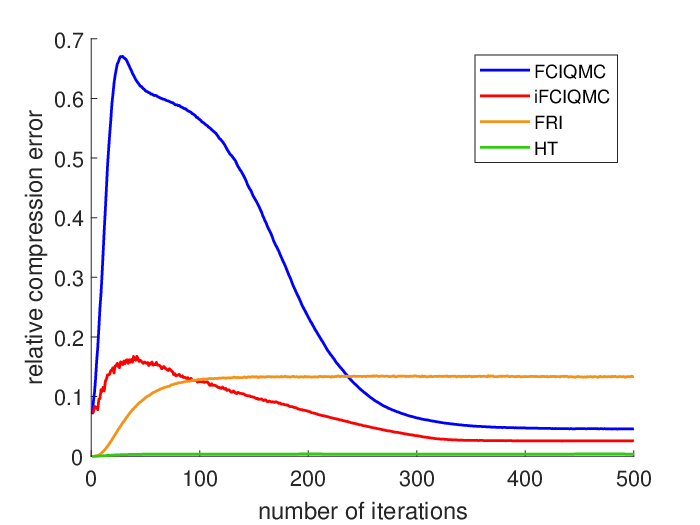
To further obtain insights of the interplay between the error per step of inexact power iteration and the convergence, we plot in Figure 2 the relative compression error and the tangent of the angle between $v_{t}$ and the exact eigenvector $u_{1}$. We observe that that FRI and HT reach convergence after about $100$ steps and FCIQMC and iFCIQMC converge after about $350$ steps; the more steps of FCIQMC and iFCIQMC are related with the first phase of the algorithm where the particle number is exponentially growing. This can be seen from Figure 2(left) as the huge error growth of the initial stage of the iterations. Only when the particle number reaches a certain level, the compression error becomes small and the power iteration convergence kicks in.

After convergence, FRI has the largest compression error and HT has the smallest. The compression error of iFCIQMC is also smaller than the one of FCIQMC. It is reasonable since HT and iFCIQMC reduce variance and thus compression error compared with the fully stochastic FRI and FCIQMC. As shown in Figure 2, in this example with the parameter choice, FCIQMC has smaller compression error than FRI; and the larger the compression error is, the further $v_{t}$ is away from the true eigenvector $u_{1}$. This agrees with the theoretical results we obtain in Theorem 1, because $\tan\theta(v_{t},u_{1})$ is controlled by the error $\xi_{t}$ at each step.

We remark that the $\tan\theta(v_{t},u_{1})$ error measure does not directly translate to the error of the projected energy estimator using say the Hartree-Fock state. In fact, we observe in Figure 1 and Table 2 that per iteration, the projected energy estimated by FRI is smaller than FCIQMC and iFCIQMC. As an explanation, in our parameter regime, the exact ground state has a large overlap with the Hartree-Fock state, so in FRI, that component is kept unchanged in the compression, while for FCIQMC and iFCIQMC, the stochastic error is more uniformly distributed over all the entries. This behavior seems more problem dependent though, as we will see in the chemical molecular examples that the MSE of FRI become comparable with FCIQMC.

4.2. Molecules

We also tested the four algorithms for some molecule examples. The FCI Hamiltonian is obtained by a Hartree-Fock calculations in a chosen chemical basis (for single-particle Hilbert space), such as cc-PVDZ. We choose Ne and $\text{H}{\vphantom{\text{X}}}_{\smash[t]{\text{2}}}\text{O}$ at equilibrium geometry as examples, which is described in Table 1. The time step is taken as $\delta=0.01$.

The convergence of projected energy error versus wall-clock time is shown in Figure 3 and Figure 4 respectively. The parameter choice of the algorithms and more quantitative comparison are shown in Table 3 and Table 4. The four algorithms also work well for molecule systems. The convergence behavior is similar to the Hubbard case.

The complexity parameter $m$ needed to achieve convergence depends on the system. The ratio $m/N$ of Ne is smaller than $\text{H}{\vphantom{\text{X}}}_{\smash[t]{\text{2}}}\text{O}$. The time cost of FRI and HT is much larger than FCIQMC and iFCIQMC, because they require the exact matrix-vector multiplication $Av_{t}$, which is still expensive although $v_{t}$ is sparse. Unlike the Hubbard case where FRI gives much smaller error, the MSE of FRI is similar to FCIQMC and iFCIQMC in these cases.

Figure 3. Convergence of the projected energy with respect to time for Ne in aug-cc-pVDZ basis

	$m$	$\lVert Av_{t}\rVert_{0}$	avg. error	std.	MSE	$\tau_{\text{auto}}$	time/iter.(s)
FCIQMC	$1.8\times 10^{6}$	-	$1.1\times 10^{-4}$	$3.8\times 10^{-5}$	$1.8\times 10^{-8}$	$12.4$	$1.5$
iFCIQMC	$1.8\times 10^{6}$	-	$7.7\times 10^{-5}$	$2.4\times 10^{-5}$	$9.6\times 10^{-9}$	$15.3$	$1.1$
FRI	$1.0\times 10^{4}$	$7.9\times 10^{6}$	$8.0\times 10^{-5}$	$4.8\times 10^{-5}$	$1.1\times 10^{-8}$	$12.3$	$11.6$
HT	$1.0\times 10^{4}$	$3.3\times 10^{6}$	$1.7\times 10^{-3}$	-	$2.8\times 10^{-6}$	-	$7.9$

Table 3. Comparison of algorithms for Ne in aug-cc-pVDZ basis

Figure 4. Convergence of the projected energy with respect to time for $\text{H}{\vphantom{\text{X}}}_{\smash[t]{\text{2}}}\text{O}$ in cc-pVDZ basis

	$m$	$\lVert Av_{t}\rVert_{0}$	avg. error	std.	MSE	$\tau_{\text{auto}}$	time/iter.(s)
FCIQMC	$6.0\times 10^{7}$	-	$4.1\times 10^{-5}$	$1.7\times 10^{-4}$	$2.1\times 10^{-9}$	$25.6$	$54.1$
iFCIQMC	$6.0\times 10^{7}$	-	$1.4\times 10^{-5}$	$5.3\times 10^{-5}$	$2.7\times 10^{-10}$	$119$	$36.6$
FRI	$1.2\times 10^{5}$	$1.6\times 10^{8}$	$2.2\times 10^{-5}$	$1.2\times 10^{-4}$	$8.9\times 10^{-10}$	$12.8$	$379.3$
HT	$1.2\times 10^{5}$	$3.4\times 10^{7}$	$1.1\times 10^{-3}$	-	$1.2\times 10^{-6}$	-	$227.0$

Table 4. Comparison of algorithms for $\text{H}{\vphantom{\text{X}}}_{\smash[t]{\text{2}}}\text{O}$ in cc-pVDZ basis

In summary, the numerical examples show that the FCIQMC, FRI and their variants can achieve convergence using much less memory and computational time compared to the standard power iteration. The stochastic algorithms FCIQMC, iFCIQMC and FRI give better estimates than the deterministic method HT in general. The numerical test also points out directions to further improve these inexact power iterations, including variance and memory cost reduction of the inexact matrix-vector multiplication and efficient parallel implementation to overcome the memory bottleneck. These will be leaved for future works.

References

- [1] (2005) Important configurations in configuration interaction and coupled-cluster wave functions. Chem. Phys. Lett. 412, pp. 121–124. Cited by: §1.
- [2] (2015) Semi-stochastic full configuration interaction quantum Monte Carlo: Developments and application. The Journal of Chemical Physics 142 (18), pp. 184107. External Links: ISSN 0021-9606, Link Cited by: §1.
- [3] (2013) Towards an exact description of electronic wavefunctions in real solids. Nature 493, pp. 365–370. Cited by: §1.
- [4] (2009) Fermion Month Carlo without fixed nodes: A game of life, death, and annihilation in Slater determinant space. J. Chem. Phys. 131, pp. 054106. Cited by: §1, §1, §3.1.1, §3.1.1, §3.1.1, §3.
- [5] (2011) Breaking the carbon dimer: The challenges of multiple bond dissociation with full configuration interaction quantum Monte Carlo methods. The Journal of Chemical Physics 135 (8), pp. 084104. External Links: ISSN 0021-9606, Link Cited by: §1.
- [6] (1974) Individualized configuration selection in CI calculations with subsequent energy extrapolation. Theoretica Chimica Acta 35 (1), pp. 33–58. External Links: ISSN 0040-5744, Link Cited by: §1.
- [7] (2010) Survival of the fittest: Accelerating convergence in full configuration-interaction quantum Monte Carlo. J. Chem. Phys. 132, pp. 041103. Cited by: §1, §1, §3.1.3.
- [8] (1993) Size-consistent self-consistent truncated or selected configuration interaction. The Journal of Chemical Physics 99 (2), pp. 1240–1254. External Links: ISSN 0021-9606, Link Cited by: §1.
- [9] (2014) Adaptive multiconfigurational wave functions. The Journal of Chemical Physics 140 (12), pp. 124114. External Links: ISSN 0021-9606, Link Cited by: §1.
- [10] (2013) Using perturbatively selected configuration interaction in quantum Monte Carlo calculations. Canadian Journal of Chemistry 91 (9), pp. 879–885. External Links: ISSN 0008-4042, Link Cited by: §1.
- [11] (1995) Estimating full configuration interaction limits from a Monte Carlo selection of the expansion space. The Journal of Chemical Physics 103 (5), pp. 1821–1828. External Links: ISSN 0021-9606, Link Cited by: §1.
- [12] (1998) Monte Carlo Configuration Interaction. Journal of Computational Physics 146 (1), pp. 181–202. External Links: ISSN 0021-9991, Link Cited by: §1.
- [13] (1991) Approximating full configuration interaction with selected configuration interaction and perturbation theory. The Journal of Chemical Physics 94 (7), pp. 5021–5031. External Links: ISSN 0021-9606, Link Cited by: §1.
- [14] (2016) Efficient heat-bath sampling in Fock space. J. Chem. Theory Comput. 12, pp. 1561–1571. Cited by: §1.
- [15] (1973) Iterative perturbation calculations of ground and excited state energies from multiconfigurational zeroth-order wavefunctions. The Journal of Chemical Physics 58 (12), pp. 5745–5759. External Links: ISSN 0021-9606, Link Cited by: §1.
- [16] (1991) Selected versus complete configuration interaction expansions. The Journal of Chemical Physics 95 (3), pp. 1877–1883. External Links: ISSN 0021-9606, Link Cited by: §1.
- [17] (2003) Direct configuration interaction and multiconfigurational self-consistent-field method for multiple active spaces with variable occupations. I. Method. The Journal of Chemical Physics 119 (18), pp. 9364–9376. External Links: ISSN 0021-9606, Link Cited by: §1.
- [18] (2015) Compressive sampling in configuration interaction wavefunctions. Molecular Physics 113 (13-14), pp. 1655–1660. External Links: ISSN 0026-8976, Link Cited by: §1.
- [19] (2017) Fast randomized iteration: Diffusion Monte Carlo through the lens of numerical linear algebra. SIAM Rev. 59, pp. 547–587. Cited by: §1, §3.2.1, §3.2.1, §3.2, §3.
- [20] (2016) iCI: Iterative CI toward full CI. Journal of Chemical Theory and Computation 12 (3), pp. 1169–1178. External Links: ISSN 1549-9618, Link Cited by: §1.
- [21] (2011) The generalized active space concept in multiconfigurational self-consistent field methods. The Journal of Chemical Physics 135 (4), pp. 044128. External Links: ISSN 0021-9606, Link Cited by: §1.
- [22] (1996) Full configuration-interaction and state of the art correlation calculations on water in a valence double-zeta basis with polarization functions. J. Chem. Phys. 104 (20), pp. 8007. External Links: Link Cited by: §4.
- [23] (2012) Semistochastic projector Monte Carlo method. Phys. Rev. Lett. 109, pp. 230201. Cited by: §1.
- [24] (2008) A sparse matrix based full-configuration interaction algorithm. The Journal of Chemical Physics 128 (14), pp. 144101. External Links: ISSN 0021-9606, Link Cited by: §1.
- [25] (2009) Importance truncation for large-scale configuration interaction approaches. Physical Review C 79 (6), pp. 064324. External Links: ISSN 0556-2813, Link Cited by: §1.
- [26] (2016) Communication: An adaptive configuration interaction approach for strongly correlated electrons with tunable accuracy. The Journal of Chemical Physics 144 (16), pp. 161106. External Links: ISSN 0021-9606, Link Cited by: §1.
- [27] (2017) Projector Quantum Monte Carlo Method for Nonlinear Wave Functions. Physical Review Letters 118 (17), pp. 176403. External Links: ISSN 0031-9007, Link Cited by: §1.
- [28] (2017) Semistochastic Heat-Bath Configuration Interaction Method: Selected Configuration Interaction with Semistochastic Perturbation Theory. Journal of Chemical Theory and Computation 13 (4), pp. 1595–1604. External Links: ISSN 1549-9618, Link Cited by: §1.
- [29] (2015) Open-Source Development Experiences in Scientific Software: The HANDE Quantum Monte Carlo Project. Journal of Open Research Software 3 (1). External Links: ISSN 2049-9647, Link Cited by: §4.
- [30] (2013) Stochastic determination of effective Hamiltonian for the full configuration interaction solution of quasi-degenerate electronic states. The Journal of Chemical Physics 138 (16), pp. 164126. External Links: ISSN 0021-9606, Link Cited by: §1.
- [31] (2016) A deterministic alternative to the full configuration interaction quantum Monte Carlo method. J. Chem. Phys. 145, pp. 044112. Cited by: §1.
- [32] (2016) A Deterministic Projector Configuration Interaction Approach for the Ground State of Quantum Many-Body Systems. Journal of Chemical Theory and Computation 12 (9), pp. 4326–4337. External Links: ISSN 1549-9618, Link Cited by: §1.
- [33] (2017) Incremental full configuration interaction. The Journal of Chemical Physics 146 (10), pp. 104102. External Links: ISSN 0021-9606, Link Cited by: §1.
- [34] (2017) Strong correlation in incremental full configuration interaction. The Journal of Chemical Physics 146 (22), pp. 224104. External Links: ISSN 0021-9606, Link Cited by: §1.