

Predicate Pairing for Program Verification
Abstract
It is well-known that the verification of partial correctness properties of imperative programs can be reduced to the satisfiability problem for constrained Horn clauses (CHCs). However, state-of-the-art solvers for constrained Horn clauses (or CHC solvers) based on predicate abstraction are sometimes unable to verify satisfiability because they look for models that are definable in a given class of constraints, called -definable models. We introduce a transformation technique, called Predicate Pairing, which is able, in many interesting cases, to transform a set of clauses into an equisatisfiable set whose satisfiability can be proved by finding an -definable model, and hence can be effectively verified by a state-of-the-art CHC solver.
In particular, we prove that, under very general conditions on , the unfold/fold transformation rules preserve the existence of an -definable model, that is, if the original clauses have an -definable model, then the transformed clauses have an -definable model. The converse does not hold in general, and we provide suitable conditions under which the transformed clauses have an -definable model if and only if the original ones have an -definable model. Then, we present a strategy, called Predicate Pairing, which guides the application of the transformation rules with the objective of deriving a set of clauses whose satisfiability problem can be solved by looking for -definable models. The Predicate Pairing strategy introduces a new predicate defined by the conjunction of two predicates occurring in the original set of clauses, together with a conjunction of constraints. We will show through some examples that an -definable model may exist for the new predicate even if it does not exist for its defining atomic conjuncts. We will also present some case studies showing that Predicate Pairing plays a crucial role in the verification of relational properties of programs, that is, properties relating two programs (such as program equivalence) or two executions of the same program (such as non-interference). Finally, we perform an experimental evaluation of the proposed techniques to assess the effectiveness of Predicate Pairing in increasing the power of CHC solving.
keywords
Program Verification, Constrained Horn Clauses, Constraint Logic Programming, Program Transformation, Relational Properties of ProgramsNote: This article has been published in Theory and Practice of Logic Programming, 18(2), 126–166, ©Cambridge University Press.
1 Introduction
Constrained Horn clauses (CHCs, for short) have been advocated by many researchers as a suitable logical formalism for the specification and the automated verification of properties of imperative programs [1, 5, 10, 30, 33, 41, 43, 45, 46]. In particular, the problem of showing partial correctness properties defined by Hoare triples [26] has a natural translation into the problem of proving the satisfiability of a suitable set of constrained Horn clauses.
Consider, for instance, the C-like program sum_upto in Figure 1, which computes the sum of the first m non-negative integer numbers:
int m, sum;
int f(int x) {
   int r = 0;
   while (x > 0) {
      r = r + x;  x--; }
   return r;
   }
void sum_upto() {
   sum = f(m);
   }
Suppose we want to prove the following Hoare triple: . This triple is valid if the following set of clauses, called verification conditions, is satisfiable:
1.
2.
3.
These clauses can be obtained in an automatic way from an interpreter of the C-like imperative language we consider and the given Hoare triple by using a technique described in the literature [1, 10, 15, 41, 43]. The predicate , which holds iff , encodes the operational semantics of the program sum_upto. Clause 1 encodes the Hoare triple, stating that if holds with (that is, the precondition holds) and (that is, is initialized to ), then (that is, at the end of the execution, the value of the variable is not smaller than the value of the variable ). Clauses 2 and 3 encode the while-loop of the function f.
Constrained Horn clauses are syntactically the same as constraint logic programs [29]. However, the term ‘constrained Horn clauses’ is mostly used in the field of program verification and, unlike ‘constraint logic programs’, it is not associated with any operational meaning. Moreover, most of the research on constrained Horn clauses is devoted to finding a model, expressible in the constraint theory, that proves the satisfiability of the clauses, whereas the operational semantics of constraint logic programs is based on a refutation procedure that looks for a proof of the unsatisfiability of the clauses. In this respect, the techniques used for finding models of constrained Horn clauses are closer to the ones proposed for the static analysis of constraint logic programs based on abstract interpretation [9, 3], where the objective is to find an over-approximation of the least model of the program.
The proof of satisfiability of sets of constrained Horn clauses is supported by CHC solvers that have been developed in recent years for various constraint theories, such as (linear or nonlinear) integer arithmetic, real (or rational) arithmetic, booleans, integer arrays, lists, heaps, and other data structures [11, 24, 25, 27, 28, 33, 39]. However, in general, since the satisfiability of constrained Horn clauses is an undecidable problem, CHC solvers may not be able to return conclusive answers.
In order to improve the effectiveness of CHC solvers, several techniques proposed by recent papers perform satisfiability preserving transformations on sets of clauses that, in some cases, derive clauses whose satisfiability is easier to prove [10, 12, 13, 14, 31, 32]. These transformations are adaptations to the task of improving the effectiveness of satisfiability checking of earlier techniques which were developed for improving the efficiency of execution of (constraint) logic programs, such as query answer transformation, specialization (or partial deduction), and unfold/fold transformations [18, 19, 36, 48, 44].
In this paper we further enhance the approach to CHC satisfiability checking based on unfold/fold transformations. Our two main contributions are the following: (1) we prove in a precise mathematical sense that the application of the unfold/fold transformation rules cannot worsen the effectiveness of CHC solvers, and actually these rules are able to strictly enlarge the set of satisfiability problems that can be solved by a given class of CHC solvers; and (2) we provide a specific strategy, called Predicate Pairing, for applying the transformation rules with the objective of improving the ability of CHC solvers to prove satisfiability.
The basic idea behind the first contribution is as follows. Similarly to what is introduced in a paper by Bjørner et al. [5], we consider the notion of the -definable model, which is a model definable in a class of first order formulas. Typically, CHC solvers (and, in particular, the solvers based on predicate abstraction) look for models in specific classes, such as linear (integer or real ) arithmetic formulas, or quantifier-free array formulas. While satisfiability is undecidable and not semidecidable, the existence of an -definable model is semidecidable, as long as the validity problem for the formulas in is decidable, and hence solvers that find an -definable model whenever it exists, can indeed be constructed. We prove that, under very general conditions on , the unfold/fold rules preserve the existence of an -definable model, that is, if the original clauses have an -definable model, then also the transformed clauses have an -definable model. The converse does not hold: there are cases where the original clauses have no -definable model, while the transformed clauses have an -definable model. In this sense the application of the unfold/fold rules may improve the effectiveness of a CHC solver that works by searching for -definable models, because the solver may be able to find an -definable model after the transformation in cases where there was no such a model before the transformation.
We also provide less general conditions under which the transformed clauses have an -definable model if and only if the original ones have an -definable model. These conditions prevent the introduction of new predicates that have recursive definitions in terms of the old predicates occurring in the original clauses. Thus, the source of the improvement of the effectiveness of the CHC solver due to the unfold/fold transformations is the introduction of one or more new predicates and the derivation of new (mutually) recursive definitions for these predicates.
The second contribution of our paper is related to the fact that, due to the already mentioned undecidability limitations, there is no universal algorithm that, starting from a set of clauses, applies the unfold/fold rules and derives a set of clauses such that, if it is satisfiable, then it has an -definable model, for some theory whose validity problem is decidable. Therefore, it should not be unexpected that the Predicate Pairing strategy we propose for guiding the use of the unfold/fold transformation rules is based on heuristics. We show that this strategy is capable, in many significant cases, of transforming sets of clauses into new, equisatisfiable sets of clauses, whose satisfiability problem can be solved by constructing -definable models, while the original sets have no -definable models. Predicate Pairing introduces a new predicate defined by the conjunction of two predicates together with a conjunction of constraints. We will explain through examples why an -definable model may exist for a conjunction of predicates, even if it does not exist for the atomic conjuncts in isolation. (Obviously, by a repeated application of Predicate Pairing, we may introduce new predicates corresponding to the conjunction of more than two old predicates.) Thus, Predicate Pairing can be viewed as an extension to constrained Horn clauses of techniques for transforming logic programs, such as the tupling unfold/fold strategy [44] and conjunctive partial deduction [17].
We will show that constraint-based reasoning is essential for guiding the introduction of the suitable pairs of predicates during the transformation process. Moreover, we will show that Predicate Pairing works well for solving many satisfiability problems that arise from the field of imperative program verification. In particular, Predicate Pairing is a crucial technique for verifying relational program properties [2], that is, properties relating two programs (such as program equivalence) or two executions of the same program (such as non-interference).
The paper is structured as follows. In Section 2 we recall the basic notions concerning constrained Horn clauses and we define the notion of an -definable model. In Section 3 we prove our results concerning the preservation of -definable models when using the unfold/fold transformation rules. In Section 4 we present the Predicate Pairing strategy and in Section 5 we show some examples of its application for verifying relational program properties. In Section 6 we report the results obtained by our implementation of that strategy by using the VeriMAP transformation system [11]. Finally, in Section 7 we discuss related work in the fields of program transformation and verification.
2 Constrained Horn Clauses
In this section we recall the basic definitions concerning constrained Horn clauses and their satisfiability, and we introduce the notion of an -definable model.
Let be a first order language with equality and be a set of predicate symbols, called the user-defined predicate symbols. Let be a set of formulas of , called the set of constraints. We assume that: (i) true, false, and equalities between terms belong to , and (ii) is closed under conjunction.
An atom is an atomic formula of the form , where is a predicate symbol in and are distinct variables. Let Atom be the set of all atoms. A definite constrained clause is an implication of the form whose premise (or body) is the conjunction of a constraint and a (possibly empty) conjunction of atoms , and whose conclusion (or head) is an atom. A constrained goal (or simply, a goal) is an implication of the form , where is a constraint and is a conjunction of atoms. A constrained Horn clause (CHC) (or simply, a clause) is either a definite constrained clause or a constrained goal. A set of constrained Horn clauses is said to be a CHC set. A constrained Horn clause Cl (or a set of clauses) is said to be ‘over ’ in case we want to stress that the constraints occurring in clause Cl (or in the set of clauses) are taken from the set of constraints. A clause is said to be linear if consists of at most one atom, and nonlinear otherwise.
We will often use the logic programming syntax and we write , instead of . We will also feel free to write non-variable terms as arguments of atoms. Thus, the clause should be viewed as a shorthand for , where is a variable not occurring elsewhere in the clause, and likewise, should be viewed as a shorthand for .
Given a formula , we denote by its existential closure and by its universal closure. By and we denote the set of variables and the set of the free variables, respectively, occurring in .
For the notions of an interpretation and a model of a first order formula we will use the standard notions and notations [40]. We fix a canonical interpretation of the symbols in . A -interpretation is an interpretation of that for all symbols occurring in , agrees with . If is the universe of , then a -interpretation can be identified with the set of atoms:
where denotes the -ary relation which is the interpretation of in . Given any set of formulas, a -interpretation is a -model of , written , if, for all formulas , holds. is -satisfiable if it has a -model. We will feel free to say satisfiable, instead of -satisfiable, when the interpretation is clear from the context. We write if, for every -interpretation , holds.
A set of definite constrained clauses is -satisfiable and has a least (with respect to set inclusion) -model, denoted [29]. Thus, if is any set of constrained Horn clauses and is the subset of the constrained goals in , then is -satisfiable if and only if .
Many CHC solvers based on predicate abstraction [5] try to check the -satisfiability of a set of constrained Horn clauses by looking for the existence of -models that are definable by formulas belonging to a given set , which is a subset of the set of constraints. This restriction when looking for models may significantly ease the satisfiability test, as shown by the following example.
Example 1
Let us assume that is the set of linear integer arithmetic (LIA) constraints, that is, equalities and inequalities between linear polynomials with integer coefficients and integer-valued variables, closed with respect to conjunction and disjunction. We also use the symbols , , , and with the usual definitions in terms of and . Let denote the usual interpretation of integer arithmetic.
Now, let us consider clauses 1–3 listed in the Introduction. The satisfiability of these clauses can be proved by looking for models that are definable by constraints in the subset of LIA, which we call 2VAR, defined by the following grammar:
where and are variables. Thus, 2VAR is the set of linear integer constraints constructed from arithmetic comparisons between at most two variables, and it is a subset of the Octagons domain often considered in the field of abstract interpretation [42]. A 2VAR-definable model of clauses 1–3 is given by interpreting the predicate as the set of triples satisfying the following constraint in 2VAR:
,
In order to show that the above interpretation indeed defines a -model, we replace the instances of by the corresponding instances of the formula in clauses 1–3, and we check that the resulting implications hold in .
This Example 1 motivates the introduction of the notion of an -definable model, which is a generalization of the one presented in the literature [5], where coincides with .
Definition 1
Let be a set of formulas of such that: (i) true, false, and equalities between terms belong to , and (ii) is closed under conjunction. Let be the canonical interpretation of the symbols in . We denote by the set of formulas and for . A symbolic interpretation is a function such that and, for every , (i) , and (ii) for every renaming substitution for [37], . We extend to conjunctions of atoms by stating that . Given a set of constrained Horn clauses over , a symbolic interpretation is an -definable model of , written , if for every clause in , holds.
Note that the symbolic interpretation of an atom is independent of the variable names occurring in that atom, and hence, for each predicate symbol , the formula is unique up to variable renaming. Note also that the definition of a symbolic interpretation is essentially equivalent to that given by Kafle and Gallagher, who define an interpretation as a set of constrained facts of the form , where is a constraint in [32]. Indeed, the set of constraints in the bodies of the constrained facts with the same head predicate can be represented as a disjunction of those constraints, and the variables occurring in the body of a constrained fact and not in its head are implicitly existentially quantified.
Clearly, if has an -definable model, then is -satisfiable. In general the converse does not hold, as shown by the following example.
Example 2
Let us continue Example 1, where the sets of constraints and are LIA and 2VAR, respectively. Let us consider the program in Figure 2, which computes the square of a non-negative integer n by summing up n times the value of n.
int n, sqr;
int g(int y, int k) {
  int s = 0;
  while (y > 0) {
    s = s + k;   y--; }
  return s;
  }
void square() {
  sqr = g(n,n);
  }
Clauses 4–6 below express the following property, which relates program sum_upto and program square: if the value of m is equal to the value of n before the execution of the programs sum_upto and square and they both terminate, then at the end of their execution the value of sqr is not smaller than the value of sum. Note that, since the programs sum_upto and square have disjoint sets of variables, the order of their execution is immaterial.
4.
5.
6.
For , the atom holds iff . Properties like the one between programs sum_upto and square are called relational properties [2]. Similarly to the verification conditions for partial correctness properties, the clauses for relational properties, also called verification conditions, can be automatically generated from the formal specification of those properties and the operational semantics of the programming language [14]. For brevity, we do not give here the details of that generation process, which is inessential for understanding the techniques presented in this paper.
Clauses 2–6 are constrained Horn clauses over LIA and they are -satisfiable. Indeed, in the least -model of clauses 2, 3, 5, 6, for all integers and with , if and hold, then holds. However, clauses 2–6 do not admit a 2VAR-definable model. Indeed, no constraint of the form , for any variable , is a consequence of , and hence we cannot infer , independently of the constraints that are consequences of . Actually, it is not difficult to see that a similar limitation holds even if we look for a LIA-definable model, rather that a 2VAR-definable model. Indeed, in order to infer the constraint one should discover quadratic relations, such as and , starting from and , respectively, and these relations cannot be expressed by linear arithmetic constraints.
3 Transformation Rules and Preservation of -definable Models
Let be a set of constraints and . A transformation sequence over is a sequence of CHC sets over , where, for is derived from by applying one of the following rules R1–R4.
Let denote the set of all the clauses, called definitions, introduced by rule R1 during the construction of the transformation sequence . Thus, .
(R1) Definition. We introduce a clause : , where: (i) newp is a predicate symbol in not occurring in the sequence , (ii) , (iii) is a non-empty conjunction of atoms whose predicate symbols occur in , and (iv) are distinct variables occurring free in . Then, we derive the new set and .
(R2) Unfolding. Let : be a clause in . Let
be the (possibly empty) set of clauses in whose head predicate is . Without loss of generality, we assume that, for . By unfolding the atom in using we derive the new set .
(R3) Folding. Let : be a clause in , where is a non-empty conjunction of atoms, and let : be (a variant of) a clause in with . Suppose that there exist a substitution and a constraint such that: (i) , (ii) , and (iii) for every variable , the following conditions hold: (iii.1) is a variable not occurring in , and (iii.2) does not occur in the term , for any variable occurring in and different from . By folding using the definition , we derive clause : . In this case we also say that is derived by folding in . We derive the new set .
(R4) Constraint Replacement. Let us consider a subset of of the form . Suppose that, for some constraints
where and . Then, we derive the new set .
Note that rule R4 enables the deletion of a clause with an inconsistent constraint in its body. Indeed, if is unsatisfiable, then with .
The following result [19] shows that the transformation rules R1–R4 derive sets of clauses that are equivalent with respect to the least -model.
Theorem 1 (Equivalence with respect to the Least -Model)
Let be a transformation sequence where, for is a set of definite clauses. Let us assume that every definition in is unfolded during the construction of this sequence (that is, for every definition , there exists , with , such that is derived from by unfolding ). Then, for every predicate and ,
if and only if .
From Theorem 1 it follows that, as we now show, the transformation rules R1–R4 derive sets of clauses that are equivalent with respect to -satisfiability.
Theorem 2 (Equivalence with respect to -Satisfiability)
Let be a transformation sequence such that every definition in is unfolded during the construction of this sequence. Then, is -satisfiable if and only if is -satisfiable.
Proof 3.3.
First we observe that is -satisfiable iff is -satisfiable. Indeed: (i) if is a -model of , then the -interpretation is a head predicate in is a -model of , and (ii) if is a -model of , then by the definition of -model, is a -model of .
Now let us consider a new sequence obtained from the transformation sequence by replacing each occurrence of false in the head of a clause by a new predicate symbol . The sequence satisfies the hypothesis of Theorem 1, and hence iff .
We have that: is -satisfiable iff is -satisfiable iff iff {by Theorem 1} iff is -satisfiable iff is -satisfiable.
Theorem 2 is not sufficient to ensure that a transformation sequence preserves the existence of an -definable model. Indeed, as shown by Example 2 in Section 2, for some set of constraints, -satisfiability does not imply the existence of an -definable model.
Now, in order to study the preservation of -models during the construction of a transformation sequence over , for , we introduce the notions of -soundness and -completeness.
Definition 3.4 (-Soundness, -Completeness).
Let be a transformation sequence. (i) If has an -definable model implies that has an -definable model, we say that the sequence is -sound. (ii) If has an -definable model implies that has an -definable model, we say that the sequence is -complete.
In order to prove the -soundness of a transformation sequence (see Theorem 3.7 below) we need the following definition and theorem.
Definition 3.5.
Let be a CHC set. A symbolic interpretation is said to be tight on if for all clauses in , , where .
For instance, given the singleton set of clauses , the symbolic interpretation that maps both and to is tight on , while the symbolic interpretation that maps to true and to is not tight on . Both and are models.
Theorem 3.6.
Let be a transformation sequence. For if has an -definable model that is tight on , then has an -definable model that is tight on .
Proof See Appendix.
The hypothesis that has an -definable model that is tight on is needed to guarantee that the folding rule replaces a conjunction consisting of constraints and atoms by a single atom which is equivalent in the given model.
From Theorem 3.6 and the fact that, if has an -definable model, then has an -definable model that is tight on , which is the empty set, we get the following result.
Theorem 3.7 (-Soundness).
Every transformation sequence is -sound.
Now we prove that, if some suitable hypotheses hold, a transformation sequence is also -complete. First, we need the following two definitions.
Definition 3.8.
An application of the unfolding rule R2 to a clause : in is said to be a self-unfolding if the predicate of is .
Definition 3.9.
Let be a transformation sequence. An application of the folding rule R3 to a clause in using a definition in is said to be a reversible folding if belongs to and is different from .
Theorem 3.10 (-Completeness).
Let be a transformation sequence over a set of constraints. Let be equal to . Suppose that: (i) no application of the unfolding rule is a self-unfolding, and (ii) every application of the folding rule is a reversible folding. Then, is -complete.
Proof See Appendix.
In Section 4 we will present the Predicate Pairing transformation strategy and we will show that it generates transformation sequences that are -sound, but not necessarily -complete (see Theorem 4.12).
Normally, -soundness is a desirable property of a transformation sequence . Indeed, suppose we have a CHC solver, call it SOLVE, that finds an -definable model of a set of clauses whenever it exists. As already mentioned, such an ideal solver exists, as long as the validity problem for the formulas in is decidable. Then, -soundness guarantees that if the satisfiability of can be proved by using SOLVE, then also the satisfiability of can be proved by using SOLVE. In other terms, the effectiveness of the solver is not worsened by the transformation.
In contrast, -completeness might not always be a desirable property. Indeed, in many cases we may want to transform clauses for which SOLVE cannot find an -definable model, because such a model does not exist, and derive equisatisfiable clauses with an -definable model which can be constructed by using SOLVE.
In practice, the existing solvers do not guarantee that they find an -definable model of a set of clauses whenever it exists. Thus, the theoretical properties of -soundness and -completeness might not hold in some cases. We will show through the experiments reported in Section 6, that these unfortunate cases are rare.
We conclude this section by showing that there are -safisfiable CHC sets that have no -definable models, and yet can be transformed, by applying rules R1–R4, into CHC sets that have -definable models.
Example 3.11.
Let us continue Example 2, where is , is LIA, and is 2VAR. Let be the set consisting of clauses 2–6.
Starting from we construct a transformation sequence , as we now indicate. First, by applying the definition rule, we introduce the following new predicate:
7.
We derive the clause set and . Now, by unfolding the atoms and of clause 7, and then performing some more unfoldings of the derived atoms, we get:
8.
9.
10.
11.
We get and . (Here and in the rest of the example, for reasons of conciseness, we feel free to avoid to list some intermediate CHC sets in the transformation sequence.) By the constraint replacement rule R4 we can remove clauses 9 and 10, whose bodies have unsatisfiable constraints, and replace clauses 8 and 11 by:
12.
13.
We get and . Then, by the folding rule R3, we fold clause 4 (in ) using clause 7 and we derive the following clause:
14.
Finally, we fold clause 13 using clause 7 and we derive the following clause:
15.
We get the final set of clauses . Now, it is easy to check that the symbolic interpretation that maps the atom to the 2VAR constraint , and the and atoms to , is a 2VAR-definable model of . This check can be done by replacing the atoms in by the corresponding symbolic interpretations, and then verifying the validity of the formulas obtained in that way by using an SMT solver for linear arithmetic, such as the popular Z3 solver [16].
Let us now make some remarks on the derivation above.
(1) The applications of the transformation rules satisfy the hypothesis of Theorem 2 and hence is -satisfiable if and only if is -satisfiable (indeed, they are both -satisfiable).
(2) The fact that has a 2VAR-definable model, while has no such model, is due to the fact that the applications of the folding rule R3 are not reversible foldings, and hence the transformation sequence does not satisfy the hypothesis of Theorem 3.10. Indeed, clause 7 occurs in , but not in . More in general, the derivation of a CHC set with an -definable model from a CHC set without an -definable model is due to the introduction of new predicates and also to the derivation (via non-reversible foldings) of clauses that constitute recursive definitions of these new predicates.
(3) Finally, note that at every step during the transformation from to we have handled linear constraints only. However, the introduction of the new predicate , defined in terms of the conjunction of and , allows us to discover linear relations between and without having to deal with nonlinear constraints.
4 Predicate Pairing
In Section 3 we have seen that by the applying unfold/fold rules, in some cases one may transform a given -satisfiable set of clauses which does not admit an -definable model, into an equisatisfiable set of clauses which admits an -definable model. Then, the -satisfiability of the set of clauses can be proved by a CHC solver that constructs an -definable model. Example 3.11 of Section 3 suggests that the crucial step in that transformation is a predicate pairing step, that is, the introduction of a new predicate, say , whose defining clause has in its body the conjunction of two atoms, one with predicate, say , and the other with predicate, say , whose definitions are provided by the original set of clauses. Indeed, the predicate pairing allows us to derive suitable relations between arguments of the conjunction of and , which cannot be expressed by using constraints on the arguments of and separately.
In general, in order to do the transformation and perform some required folding steps, it may be necessary to introduce, by predicate pairing, more than one definition. The introduction of these new definitions is a major issue in the case where the predicates to be paired should be chosen from the various predicates occurring in the conjunction of several atoms in the body of a clause. In particular this issue arises when predicates are defined by nonlinear clauses, and hence their repeated unfolding may generate unbounded conjunctions of atoms.
In this section we will present a strategy, called Predicate Pairing, for making the choice of the predicates to be paired. This strategy, which is realized by Algorithm 1, takes as input a set of clauses and derives a new, equisatisfiable set of clauses, which by Theorem 3.7 is guaranteed to admit an -definable model, whenever the original clauses had one. Actually, as we will show, in many interesting cases the Predicate Pairing strategy constructs new sets of clauses for which a CHC solver is able to construct one such model, while the same solver is unable to do so for the original set of clauses. We present the Predicate Pairing strategy with the help of an example. Suppose that we are given the following specification of (a variant of) the Ackermann function:
let Eq be .
(i) occurs in , and (ii) occurs in do
(ii) is a conjunction of atoms, such that:
for all atoms and in , whose predicates occur in and , respectively, we have that do
for some substitution , we can fold in clause using ,
then
- (i)
newp is a predicate symbol not occurring elsewhere,
- (ii)
, and
- (iii)
e is the conjunction of the equalities in Eq;
S1.
S2.
S3.
and the following two programs each of which implements that specification:
int ackermann1(int m, int n) {
    if (m =< 0) { return n+1; }
    else if (m > 0 && n = 0) { ackermann1(m-1,1); }
    else if (m > 0 && n > 0) { ackermann1(m-1,ackermann1(m,n-1)); }
  }
int ackermann2(int m, int n) {
  while (m > 0) {
    if (n == 0) { m = m-1;   n = 1; }
    else { n = ackermann2(m,n-1);   m = m-1; }
  }
  return n+1;
}
We want to prove the equivalence of these two implementations, in the sense that, for all non-negative integers and , ackermann1(m,n) returns the same integer returned by ackermann2(m,n).
Given the programs ackermann1(m,n) and ackermann2(m,n), we first generate the following two sets and of clauses that encode the operational semantics of the programs. These sets of clauses can be derived by specializing the interpreter of the imperative language with respect to the programs [15].
- 1.
- 2.
- 3.
- 4.
- 5.
- 6.
- 7.
- 8.
The equivalence of the functions computed by the programs for ackermann1 and ackermann2 is expressed in terms of the predicates defined by clauses 1–8 as follows: for all integers , , , , we have that if , , , , and and both hold, then holds. Thus, given the clause:
- 9.
-
the proof that and are equivalent is reduced to the construction of a model for clauses 1–9 (note that the constraint in clause 9 states that the values returned by the two programs are different).
Now we have that no CHC solver that constructs LIA-definable models, can prove the satisfiability of clauses 1–9. Indeed, in order to make that proof, the solver should discover that the atoms and imply the two equalities and , respectively, where ackermann is the function specified by equations –, and these equalities cannot be expressed as linear integer constraints.
Thus, in order to allow a CHC solver to construct a LIA-definable model for clauses 1–9, one should avoid reasoning on the two predicates and in a separate way, and instead, one should reason on the conjunction of those predicates. Indeed, in what follows we will derive for that conjunction a new, equisatisfiable set of clauses that has a LIA-definable model. In this new set of clauses we will discover suitable LIA constraints relating the arguments of the predicates and . Using these constraints the CHC solver Z3 can show the existence of a LIA-definable model for clauses 1–9, thereby proving the desired equivalence between programs and .
This new set of clauses will be derived from clause 9 by applying a sequence of transformation rules according to the Predicate Pairing strategy, as indicated in Algorithm 1. The algorithm takes as input a set of clauses , that is, in our case, and produces as output a new set of clauses by applying the unfolding, definition, and folding rules. During the application of that strategy we silently apply the constraint replacement rule to remove clauses which have unsatisfiable constraints in their body.
First iteration of the body of the while-loop of Predicate Pairing.
Since , occurs in , and occurs in , we start off by unfolding and in clause 9. These unfoldings correspond to a symbolic evaluation step of each of the two atoms. We get:
- 10.
Then in order to fold clause 10, we introduce the following definition clause 11 which pairs together the atoms with predicate occurring in and predicate occurring in . In the body of this definition we have the equality constraints and between the arguments of and .
- 11.
The definition of is then used for replacing, by folding, the conjunction of the atoms with predicates and in the body of clause 10. Thus, from clause 10, by folding, we derive:
- 12.
Second iteration of the body of the while-loop of Predicate Pairing.
Since , occurs in , and occurs in , we have to perform a second iteration of the body of the while-loop of the Predicate Pairing.
We unfold the atoms with predicate and in the premise of clause 11, and we get the following three clauses:
- 13.
- 14.
- 15.
Clause 13 need not be folded because it has no atoms in its body. Clause 14 can be folded using clause 11 (the conditions for folding given in Section 3 are indeed satisfied), and we get:
- 16.
Clause 15 should be folded, but first we need to choose the atoms to be paired together. According to our goal of proving a relation between the arguments of and , we should pair together an atom with an atom. However, the choice of the atoms to be paired can be made in different ways because in clause 15 there are two atoms and two atoms. The strategy we propose looks at the arguments of the atoms and selects the two atoms which share a maximal number of equality constraints holding between an argument of and an argument of .
According to this strategy we have that should be paired with because these two atoms share the two equalities and (this last equality follows from ), while shares no equalities with . Moreover, shares one equality only, namely (this equality follows from ) with ). Thus, we pair with and then we take clause 11 for folding these two atoms.
In order to fold the other two atoms occurring in clause 15, that is, and , we introduce the following clause:
- 17.
- 18.
-
-
The basic idea of our pairing strategy is that the atoms that are paired together, having some of their arguments equal, have a somewhat synchronized behavior and this synchronization may determine, for the other arguments, the existence of simple relations that are easy to express in the theory of constraints one considers.
At this point of the application of the Predicate Pairing strategy we have that , , and .
Third iteration of the body of the while-loop of Predicate Pairing.
Since and clause 17 has the atom that occurs in and the atom that occurs in , we have to perform a new iteration of the body of the while-loop of the Predicate Pairing.
In clause 17 we unfold once the atom with predicate and the atom with predicate , and we get:
- 19.
- 20.
- 21.
- 22.
- 23.
- 24.
In order to fold clause 21, first we select the two atoms with the predicates to be paired. We have that shares one equality with , that is, (this equality follows from ), and shares no equalities with . Hence we select the atoms and in the body of clause 21, and we fold that clause by using clause 17, thereby deriving the following clause:
- 25.
Since no new iteration of the body of the while-loop of the Predicate Pairing is required. Thus, the application of that strategy terminates. The resulting set of clauses is .
Now, the CHC solver Z3, when given as input the set TransfCls of clauses, constructs a LIA-definable model of TransfCls. In particular, it constructs a LIA-definable model of clause 12 by inferring that implies , which together with , implies , and hence the body of the clause is shown to be false.
By Theorem 2 the existence of a LIA-definable model for TransfCls entails that clauses 1–9 have a -model, and this concludes the proof that programs ackermann1 and ackermann2 are equivalent.
We end this section by stating some results about the Predicate Pairing strategy. First, we have that Predicate Pairing always terminates because the number of new predicate definitions that can be introduced is bounded by the number of different conjunctions of the form , where and are atoms whose predicates occur in , and is a conjunction of equalities between variables in . Hence, the number of executions of the body of the while-loop of Predicate Pairing is at most .
It is easy to see that the sequence of applications of the transformation rules performed by the Predicate Pairing strategy constructs a transformation sequence where every definition in Defs is unfolded at least once. Thus, from Theorem 2, which states the equivalence with respect to -satisfiability, and Theorem 3.7, which states the preservation of -definable models, we get the following result.
Theorem 4.12 (Termination and soundness of the Predicate Pairing strategy).
Let the sets , , and of clauses be the input of the Predicate Pairing strategy. Then the strategy terminates and returns a set TransfCls of clauses such that:
(i) is -satisfiable iff TransfCls is -satisfiable, and
(ii) if has an -definable model, then TransfCls has an -definable model.
Finally, note that the application of the Predicate Paring strategy may be iterated, and hence, at the end of the transformation of a set of clauses, more than two predicates may turn out to be tupled together.
5 Case Studies: Relational Program Properties
In this section we illustrate the application of the Predicate Pairing strategy to some relevant classes of relational program properties. In particular, we have considered the following classes of properties: (i) the equivalence of programs implementing nonlinear and/or nested recursive functions, (ii.1) the injectivity of programs, (ii.2) the monotonicity of programs, (ii.3) the functional dependence of programs, (iii) non-interference of programs, (iv) equivalence of loop-optimized versions of programs with respect to the corresponding non-optimized versions, and (v) the equivalence of programs that manipulate integer arrays. We will consider these classes of properties in separate subsections.
Now we briefly show how to encode relational properties between the executions of two programs P and Q [14]. We assume that the operational semantics of programs P and Q is represented by predicates and , where and represent (tuples of) input values, and and represent (tuples of) output values, respectively. As already mentioned in the previous sections, the clauses defining and can be derived by specializing the interpreter of the imperative language with respect to the programs [15].
Let us now consider the relational property stating that, if the constraint holds before the execution of P and Q and the execution of these programs terminates, then the constraint holds after the execution. This property can be verified by testing the satisfiability of the CHC set consisting of the clauses defining predicates and , together with the following clause:
RP:
where is a constraint which is equivalent to the negation of 11 1 If the constraint language has no negation symbol, but the negation of a constraint is equivalent to a disjunction of constraints, as in the case of LIA, then the relational property can be encoded by a set of clauses..
The application of our method based on the use of the Predicate Pairing strategy, is often crucial for solving satisfiability problems that encode relational program properties. In Section 6 we will discuss the results we have obtained in an extensive experimental evaluation that we have conducted.
5.1 Functions with Nonlinear and/or Nested Recursion
Similarly to what has been considered in Section 4, where we have presented two imperative programs implementing the Ackermann function specification and then proved their equivalence, in this section we consider various equivalence problems for pairs of imperative programs implementing some functional specifications. In each pair one imperative program uses recursion only and the other one uses recursion and iteration.
The operational semantics of the two imperative programs is encoded using two distinct sets of CHCs, each defining a predicate for each program. The recursive structure of these predicate definitions mirrors the control flow of two imperative programs.
Let us consider two predicates and that encode the operational semantics of the two imperative programs, say and , implementing a given function specification. The equivalence between and holds if, under some precondition on the input values, and define the same input/output relation. This property holds if the following clause, together with the set of clauses defining the predicates and , is satisfiable:
EQ:
where: (i) , represent tuples of input values, (ii) , represent tuples of output values, and (iii) is a precondition on the input values. The reader may note that clause EQ is an instance of clause RP defining the general relational property. Note also that clause 9 in Section 4, encoding the equivalence relation between the two implementations of the Ackermann function, is an instance of EQ.
We have considered equivalence problems for imperative programs implementing nonlinear recursive functional specifications, that is, functional specifications with two or more recursive calls that depend on the same call (as in the case of the Fibonacci function). Also, several of these specifications have nested recursions, that is, they have recursive calls that are arguments of other recursive calls (as in the case of the Ackermann function), thus making the verification problem more challenging.
In particular, in our experiments we have considered the following specifications of variants of the Ackermann function22 2 http://mrob.com/pub/math/ln-2deep.html. (Here and in the other function definitions we assume that and are non-negative integers.)
(1) Original version by W. Ackermann:
, , ,
,
(2) Variant by H. Edelsbrunner:
, , ,
(3) Variant by R. Robinson (we have used this variant in Section 4):
, ,
(4) Variant by R. Péter:
, ,
Note that, these variants of the specification of the Ackermann function actually correspond to pairwise different functions. Indeed, we have that for all , and for all .
Additionally, we have considered some other equivalence problems for pairs of imperative programs encoding the following functional specifications:
(5) a variant of the Sudan function:
, ,
(6) the function:
,
(7) the function:
, ,
(8) the McCarthy 91 function: if then else
(9) the Dijkstra fusc function:
, , ,
, and
(10) a function that computes the minimum number of moves needed for the solution of the towers of Hanoi problem.
Our strategy turns out to be very effective in increasing the ability of the CHC solver to prove the satisfiability, or the unsatisfiability, of the clauses encoding the considered problems. As already mentioned, the main reason for this effectiveness is due to the fact that, by pairing together two atoms, the Predicate Pairing strategy often enables the discovery of relations between some of their arguments.
5.2 Monotonicity, Injectivity, and Functional Dependence
Some interesting classes of relational properties we have considered are those of monotonicity, injectivity, and functional dependency. These notions relate two different terminating executions of the same program on two distinct input values, say and , computing the output values, say and , respectively. The definition of these properties are derived in a straightforward manner from those of the mathematical functions.
In particular, monotonicity properties state that the application of the program on ordered input values produces ordered output values. For example, a typical monotonicity property is the following: if , then .
Injectivity properties state that any two executions of the same program on different inputs produce different outputs, that is, if , then .
Functional dependence properties state that the output of a program is a function of (a possibly proper subset of) its input values: for instance, if , then .
In particular, let us consider the following constrained Horn clauses encoding the operational semantics of a given imperative recursive program Fib that computes the Fibonacci numbers:
where the first argument of fib encodes the input and the second argument of fib encodes the output. Then, the above mentioned properties of monotonicity, injectivity, and functional dependence of the program Fib can be checked by testing the satisfiability of the following clauses:
(Monotonicity)
(Injectivity)
(Functional Dependence)
Note that the above clauses are all instances of clause RP encoding the general relational property.
Based on this example, the reader will not find it difficult to express monotonicity, injectivity, and functional dependence for other given imperative programs. We have successfully verified these properties for programs computing: (i) the sum of two numbers (by iterated increment), (ii) the product of two numbers (by iterated addition), and (iii) the square and the cube of a number (by iterated addition). We have also considered some more programs containing simple, sequential, or nested while-loops, possibly combined with conditionals.
5.3 Non-interference
Non-interference is a property that guarantees information-flow security. It can be viewed as a variant of the functional dependence property as we now indicate.
Let us consider an imperative program whose variables are partitioned into a set of public variables (or low security variables) and a set of private variables (or high security variables). We say that satisfies the non-interference property if any two terminating executions of , starting with the same initial values of the public variables, but possibly with different values of the private variables, compute the same values of the public variables. Thus, if a program satisfies the non-interference property, an attacker cannot acquire information about the private variables by observing the input/output relation between the public variables, which are functionally dependent on the public input variables only.
To clarify the ideas, let us consider the following simple imperative program :
while (high >= 1) { high = high-1; low = high; }
where low is a public variable and high is a private variable. Program violates the non-interference property because there exist two different executions starting with identical values of the variable low and terminating in configurations having different values for variable low. Indeed, if initially we have that high is at least 1, then the body of while-loop is executed and the final value of low will be 0, otherwise the value of low is left unchanged.
The non-interference property for program can be verified by checking the satisfiability of the following set of clauses:
where: (i) the predicate encodes the input/output relation among the variables of program , (ii) the variables and encode the values of the variables low and high at the beginning of the while-loop, and (iii) OutL encodes the value of the variable low at the end of the while-loop. Note that the set of clauses shown above is unsatisfiable because program violates the non-interference property.
The reader may note that the first clause, encoding the non-interference property for program , is an instance of clause RP defining the general relational property. The encoding of the non-interference property for other programs can be done in a similar way.
The following program is representative of a class of programs for which we have successfully verified that the non-interference property holds:
low1 = low2; low1 = low1 + f(high); low1 = low1 - g(high,low1);
where: (i) low1 and low2 are public variables, high is a private variable, and (ii) f and g are two functions defined as follows:
int f(int m) {
  int i = 0, s = 0;
  while (i <= m) { s += i+m; i++; }
  return s;  }
int g(int m, int n) {
  int i = 0, s = 0;
  if (n <= m) { while ( i<= n) { s += i+m; i++; } } ;
  while (i <= m) { s += i+m; i++; }
  return s; }
Note that, in the program the functions f and g compute the same value. This program does satisfy the non-interference property, and thus the corresponding set of clauses is satisfiable. Indeed, in the program the public variable low1 is first incremented and then decremented by the same value, which, however, is computed by the distinct, yet equivalent functions f and g, which take the private variable high as input.
5.4 Loop Optimizations
Modern compilers often perform a series of optimizations for producing a new program that is semantically equivalent to an old program, but whose execution is faster, or requires less memory, or has lower energy consumption.
By applying our method we have successfully verified equivalence properties between some imperative programs and their optimized versions [38]. The CHC encoding of program equivalence is the one defined by clause EQ in Section 5.1. For instance, we have proved the equivalence of the following program:
while (i < n) {
   if (n > 5) { a = a+n;   i = i+1; }
      else    { a = a+1;   i = i+1; }
}
and the one derived from it by the loop unswitching optimization:
if (n > 5) { while (i < n) { a = a+n;   i = i+1; } }
   else    { while (i < n) { a = a+1;   i = i+1; } }
where the conditional statement occurring in the while-loop is moved outside the loop, so that the evaluation of the conditional expression is performed only once, instead of being performed at each loop iteration.
We have also considered some specific instances of other equivalence problems relating original, non-optimized programs to new programs obtained by applying the following loop optimizations:
(i) loop fission, that splits the commands occurring in a loop in two blocks that are then executed by two consecutive, independent loops;
(ii) loop fusion, that merges the commands occurring in consecutive loops and executes them in a single loop;
(iii) loop reversal, that executes the commands occurring in a loop, in a new loop where the iteration proceeds in reversed order with respect to the order of the original loop;
(iv) strength reduction, that replaces iterated expensive computations in a loop by cheaper ones (for instance, replacing multiplication by a loop index with addition); and
(v) code sinking, that moves code occurring immediately before or after a loop inside the loop itself, possibly using conditionals for keeping the semantics of the program unaltered.
We have also considered other loop optimizations, including loop tiling, loop aligning, loop pipelining as well as other optimizations for removing redundant assignments, expression evaluations, and conditionals.
5.5 Array-manipulating Programs
We have applied our verification method to relational properties of imperative programs manipulating integer variables and integer arrays.
Let us first introduce some preliminary notions. An integer array a (or an array, for short) is a finite sequence of integers whose length, called the dimension of the array, is denoted . An atomic array constraint is either read, denoting that the -th element of the array is the integer , or write, denoting that, for , if , then the -th element of a is equal to the k-th element of b, and if , then the -th element of is the integer .
The read and write constraints satisfy the following implicative axioms [6], whose variables are assumed to be universally quantified at the front:
(array congruence)
(read-over-write)
(read-over-write)
For example, the operational semantics of the following imperative program which acts on the array a:
  i = 1;   a[0] = 3;
  while ( i < n ) { a[i] = a[i-1]+2;  i++; }
can be represented by the following set of CHCs:
In these clauses: (i) the predicate encodes the while-loop, (ii) its arguments , and encode the values of variables , and , respectively, at loop entry, and (iii) encodes the value of a at loop exit.
Now we show an example of an equivalence property between array manipulating programs that has been proved by using our method based on the Predicate Pairing strategy. Let us consider the programs and shown in Table 1, where program is obtained from program by applying the loop-pipelining optimization, a commonly used technique for enabling instruction-level parallelism at the hardware level.
| Program | Program |
|---|---|
   i=0;
   while (i < n) {
      a[i]++;
      b[i] += a[i];
      c[i] += b[i];
      i++;
   }
|
   i = 0;
   a[0]++;
   b[0] += a[0];
   a[1]++;
   while ( i < n-2 ) {
      a[i+2]++;
      b[i+1] += a[i+1];
      c[i] += b[i];
      i++;
    }
   c[i] += b[i];
   b[i+1] += a[i+1];
   c[i+1] += b[i+1];
|
The equivalence between programs and with respect to the output array c, is expressed by the following clause (which is an instance of clause EQ of Section 5.1):
:
where represents the input/output relation of the source program , and in particular, is the value of the integer variable n, is the value of the array a at the beginning of program execution, and is the value of the array c at the end of program execution. Similarly, represents the input/output relation of the optimized program .
Thus, by proving the satisfiability of the set of clauses consisting of together with the clauses defining and , we have been able to prove that programs and produce identical values for the array c as output, when provided with identical values for the array a as input.
6 Experimental Evaluation
In this section we present the experimental evaluation we have performed for assessing the effectiveness of the Predicate Pairing strategy (PP strategy, for short) presented in Section 4.
Implementation.
We have implemented Algorithm 1 by using the VeriMAP system [11], which is a tool for software model checking based on transformation techniques for CHCs. Then we have used the SMT solver Z3 [16] for checking the satisfiability of the clauses generated by VeriMAP . In particular, we have used Z3 version 4.5.0 with the Duality fixed-point engine [39], which provides support for constraints defined on linear integers and integer arrays.
Our prototype implementation consists of two components: (1) a module that realizes Algorithm 1, and (2) a module that translates the generated CHCs into the SMT-LIB format which is the format accepted by Z3 (see Figure 3). The VeriMAP system also provides a front-end module (T) that takes a pair of C programs, together with a relational property to be verified, and translates them into the CHCs that encode the verification problem [14].
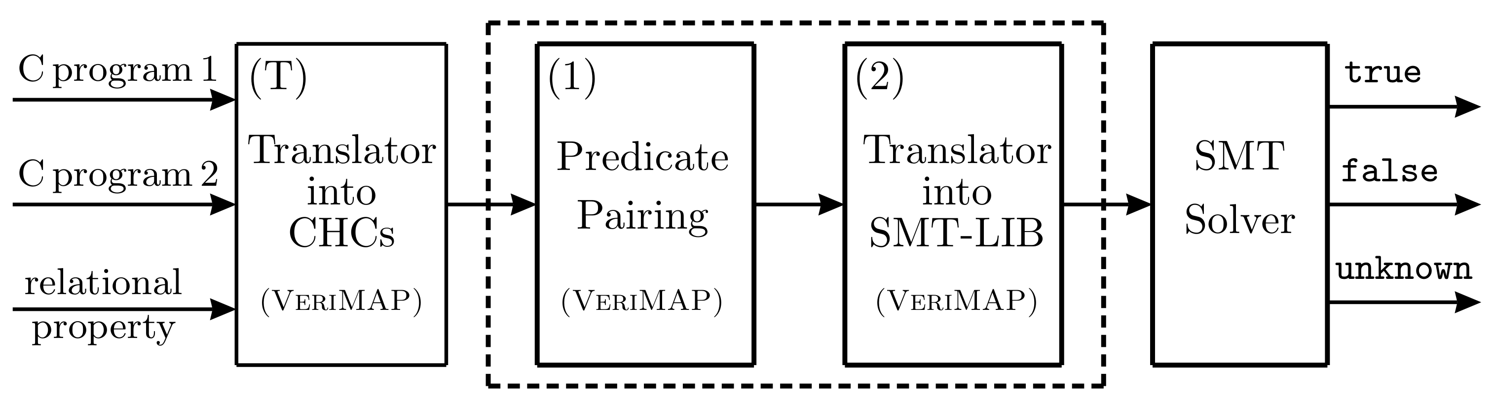
Verification problems.
We have considered a benchmark33 3 The benchmark set can be found at http://map.uniroma2.it/predicate-pairing of 163 sets of CHCs (153 of which are satisfiable and the other 10 are unsatisfiable), representing verification problems (all acting on integers and 14 of them acting on integer arrays), which refer to relational properties of small, yet non-trivial, imperative programs mostly taken from the literature [2, 4, 21, 12, 14, 38].
We have considered the following categories of relational verification problems. (1) The category nlin, which refers to equivalence properties between programs implementing functions with nonlinear and/or nested recursion. For instance, we have verified the equivalence of two programs for computing the Ackermann function (see the running example presented in Section 4 and the examples of Section 5.1). (2)–(6) The categories mon, inj, fun, nint, and lopt, which refer to monotonicity, injectivity, functional dependence, non-interference, and loop optimizations problems, respectively (see Section 5). (7) The category ite, which refers to equivalence properties and inequality properties relating two iterative programs acting on integers (by an inequality property we mean that the values computed by the programs are related by ). (8) The category arr, which refers to equivalence and inequality properties between iterative programs acting on integer arrays. (9) The category rec, which refers to equivalence properties between recursive programs. (10) The category i-r, which refers to equivalence properties between an iterative program and a (non-tail) recursive program. For example, we have verified the equivalence of the iterative and recursive versions of programs for computing: (i) the greatest common divisor of two integers, and (ii) the -th triangular number, that is, . (11) The category comp, which refers to equivalence and inequality properties between programs that contain compositions of different numbers of loops acting on integers (3 problems) and integer arrays (7 problems). (12) The category pcor, which refers to partial correctness properties of an iterative program with respect to a recursive functional postcondition [12].
Technical resources.
The experimental evaluation has been performed on a single core of an Intel Core Duo E7300 2.66GHz processor with 4GB of memory running Ubuntu. For all problems we have set the timeout limit of 300 seconds.
Experimental processes.
We have considered the following two experimental processes. (E1) The first experimental process consists in running Z3 for checking the satisfiability of the original sets of CHCs that encode the verification problems. (E2) The second experimental process consists in running Algorithm 1 on the original sets of CHCs for each verification problem, and then running Z3 for checking the satisfiability of the derived CHCs. In this second process the PP strategy has been iterated (see the end of Section 4), if more than one pair of atoms was present in the bodies of the original sets of clauses. In particular, PP has been iterated for 24 sets of CHCs, in total, belonging to categories nint, arr, comp, and pcor.
| Problems | Z3 before PP | PP | Z3 after PP | ||||
| Category | |||||||
| (1) | nlin | 13 | 4 | 16.11 | 25.80 | 13 | 13.12 |
| (2) | mon | 18 | 1 | 1.04 | 2.27 | 12 | 3.72 |
| (3) | inj | 11 | 0 | – | 1.36 | 8 | 1.39 |
| (4) | fun | 7 | 4 | 1.39 | 1.24 | 7 | 1.48 |
| (5) | nint | 18 | 3 | 0.27 | 55.80 | 17 | 41.33 |
| (6) | lopt | 20 | 2 | 4.83 | 2.98 | 15 | 10.71 |
| (7) | ite | 22 | 5 | 26.67 | 4.53 | 18 | 17.01 |
| (8) | arr | 6 | 1 | 7.45 | 2.04 | 5 | 3.25 |
| (9) | rec | 15 | 6 | 2.89 | 1.50 | 13 | 4.28 |
| (10) | i-r | 4 | 0 | – | 0.65 | 3 | 1.02 |
| (11) | comp | 10 | 0 | – | 16.35 | 7 | 6.46 |
| (12) | pcor | 19 | 5 | 83.93 | 17.84 | 17 | 17.65 |
| Total number | 163 | 31 | 144.58 | 132.36 | 135 | 121.42 | |
| Average Time | 4.66 | 0.81 | 0.90 | ||||
Results.
The results of the experimental evaluation are summarized in Table 2. The times reported are the CPU seconds spent in user mode and kernel mode by (i) VeriMAP for transforming the clauses, and (ii) Z3 for checking their satisfiability. The times required for translating the CHCs into the SMT-LIB format (this translation is necessary for running Z3) are: 6.39 seconds for the first experimental process E1, and 22.59 seconds for the second experimental process E2. Those translation times are not very high with respect to the solving times which are 144.58 seconds and 121.42 seconds, respectively.
As expected, the use of the PP strategy significantly increases the number of problems that are solved by Z3. In particular, the number of solved problems increases from 31 (Total of Column ) to 135 (Total of Column ). Note, however, the PP strategy can derive a set of clauses which is larger than the original set. In our benchmark we have observed that size increases of about 2.16 times on average.
Note also that the PP strategy increases the efficiency of the satisfiability check. Indeed, the average time taken to run PP and then Z3 (1.88 seconds) is lower than the average time taken to run Z3 on the original set of clauses (4.66 seconds). Although we have proved that the application of the PP strategy preserves all LIA-definable models, in our experiments we have found three problems which Z3 was able to solve before the application of the PP strategy (i.e., in the first experimental process), and it was no longer able to solve, within the given time limit, after the application of the PP strategy (i.e, in the second experimental process). This phenomenon may be due to the fact that the termination of the algorithms implemented by the Z3 solver is sensitive to the syntactic form of the input clauses, and the PP strategy modifies that form. Further work is needed to improve the termination behavior of the solver.
Finally, we would like to point out that the application of the PP strategy does not decrease the efficiency of the whole verification process. If we consider only the 28 problems for which Z3 is able to solve both before and after the application of the PP strategy, the average time taken to run PP and then Z3 (1.58 seconds) is slightly lower than the time taken by Z3 alone (1.77 seconds).
7 Related Work and Conclusions
The basic idea behind the Predicate Pairing transformation strategy for constrained Horn clauses is that, by finding a recursive definition of a predicate denoting the conjunction of two atoms, it is often possible to infer relations among the variables occurring in the two atoms which would have been impossible to discover by considering each atom separately.
Techniques for transforming logic programs by deriving new predicates defined in terms of conjunctions of atoms have been largely studied. Let us recall, for instance, the well-known tupling transformation strategy [44] and the conjunctive partial deduction technique for logic program specialization [17]. The main objective of tupling and conjunctive partial deduction is the derivation of more efficient logic programs by avoiding multiple traversals of data structures and repeated evaluations of predicate calls, and by producing specialized program versions.
Thus, Predicate Pairing shares with tupling and conjunctive partial deduction the idea of promoting a conjunction of atoms to a new predicate. However, in this paper we have shown that the application of this idea to constrained Horn clauses can also play a key role in improving the effectiveness of CHC solvers for proving properties of imperative programs, besides the optimization of the execution of logic programs, which is the objective of tupling and conjunctive partial deduction. This is the case especially when the CHC solvers are required to test the satisfiability of clauses that encode relational program properties, that is, properties that relate two programs, or two executions of the same program. Indeed, as shown by many examples considered in this paper, state-of-the-art solvers often fail to prove the satisfiability of sets of clauses encoding relational properties because they can only infer relations among the variables of individual atoms.
We have considered CHC solvers that prove satisfiability by using predicate abstraction, that is, by looking for models that are definable in a specific class of constraints [5]. We have shown that, in principle, the Predicate Pairing strategy cannot worsen the effectiveness of the CHC solver. Indeed, we have proved a very general result concerning the unfold/fold transformation rules used by the strategy: if a set of clauses is transformed by applying the unfold/fold rules, and the original set of clauses has an -definable model, then also the transformed set of clauses has an -definable model. Thus, if the CHC solver is able to find an -definable model whenever it exists (and this is indeed possible if the validity problem for the constraints in is decidable), then every set of clauses that can be proved satisfiable by the solver before the transformation, will also be proved satisfiable by the solver after the transformation. We have shown that, in practice, for the Z3 solver this property is guaranteed with very few exceptions.
We have also given some restrictions on the use of the rules that guarantee that the converse of the above property holds, that is: if a set of clauses is transformed by applying the unfold/fold rules, and the transformed set of clauses has an -definable model, then also the original set of clauses has an -definable model. However, this property is not always desirable. Indeed, the fact that in some cases Predicate Pairing is able to transform (satisfiable) clauses that do not have an -definable model into clauses that have an -definable model, may be a great advantage. Indeed, this means that while a CHC solver that looks for -definable models is not able to prove the satisfiability of the original clauses, the same solver may be able to prove the satisfiability of the transformed clauses.
The study of the properties that relate unfold/fold transformations and the existence of -definable models is not present in the literature on tupling and conjunctive partial deduction.
Then, we have presented an algorithm that implements the Predicate Pairing strategy. One of the novel points of this algorithm with respect to tupling and conjunctive partial deduction is that it realizes a heuristic to choose the appropriate atoms to be paired together in a new predicate definition, by maximizing the number of equality constraints that relate the variables occurring in a pair of atoms. This heuristic is crucially needed when dealing with nonlinear clauses that, by unfolding, may generate clauses with more than two atoms in their body. We have implemented our algorithm on the VeriMAP transformation and verification system [11], and we have evaluated its effectiveness on a benchmark of over 160 problems encoding relational properties of small, yet nontrivial C-like programs. The properties were of various kinds, including equivalence, injectivity, functional dependence, and non-interference (a property of interest for enforcing software security). The results show that the use of Predicate Pairing as a preprocessor greatly improves the ability of the Z3 CHC solver (with the Duality fixed-point computation engine [39]) to prove satisfiability.
Several transformation-based techniques for constrained Horn clauses, or constraint logic programs, have been proposed as a means of facilitating program verification. Many of them are non-conjunctive specialization techniques, which work by propagating the constraints occurring in the goal, thereby producing clauses with strengthened constraints in their bodies [1, 10, 15, 12, 31, 32, 41, 43]. Even if specialization techniques have been shown to be very successful, in most cases they cannot achieve the same effect as Predicate Pairing. Indeed, as already mentioned, Predicate Pairing works by introducing new predicates corresponding to conjunctions of old predicates, whereas non-conjunctive specialization can only introduce new predicates that correspond to instances of old predicates. We have experimentally checked that most of the problems considered in Section 6 cannot be solved via (non-conjunctive) specialization alone. Due to lack of space we have not reported these results.
The query-answer transformation (and variants thereof) is another pre-processing technique that is sometimes applied before performing satisfiability tests using CHC solvers [10, 31, 32]. The aim of this transformation is to simulate the top-down, goal oriented evaluation of the clauses in a bottom-up framework. The results we have presented here, showing that Predicate Pairing is able to transform clauses without an -definable model into clauses with an -definable model, are independent of the evaluation strategy adopted by the CHC solvers, and hence the query-answer transformation and the Predicate Pairing strategy should be viewed as orthogonal techniques.
Predicate Pairing is an extension of the Linearization transformation, whose objective is to transform a set of linear clauses (that is, clauses with at most one atom in their body) together with a nonlinear goal, into a set of linear clauses and linear goals [13]. The Predicate Pairing strategy does not need any linearity assumption, and indeed in Sections 4, 5, and 6 we have shown that this strategy can solve several verification problems encoded by sets of nonlinear clauses. It has also been shown that Linearization preserves the existence of LIA-definable models [13]. Here we have generalized this result by proving that the application of the unfold/fold transformation rules, independently of the strategy, preserves the existence of -definable models, for any class of constraints.
The Predicate Pairing algorithm presented here is an improvement of the one reported in previous work presented at the SAS Symposium [14]. Indeed, as already mentioned, here we use an equality-based heuristic to choose the appropriate atoms to be paired together, and this technique has been shown very effective in practice for handling nonlinear clauses. Also the case studies and the benchmark set we consider in the present paper are much larger, and include verification problems such as non-interference, correctness of loop optimizations, and equivalence of nonlinear recursive programs that have not been considered in our SAS paper [14]. Neither in that paper there are general results concerning the preservation of -models.
Bjørner et al. have shown that unfolding preserves -definable models provided that the set of constraints admits Craig interpolation [5]. In the present paper we have generalized this result by considering also other transformations, and in particular folding, and we dropped the assumption about Craig interpolation. Moreover, we assume that is a subset of the set of constraints over which the clauses are defined, while Bjørner et al. take to be equal to . Our generalization is significant because sometimes CHC solvers that make use of predicate abstraction look for models defined in subsets of the constraints used for the clauses, such as the popular domain of the octagons [42].
The problem of verifying relational properties is very relevant in the context of software engineering. Indeed, during software development it is often the case that one modifies the program text, and hence needs a proof that the semantics of the new program version has some specified relation to the semantics of the old version. This kind of proof is sometimes called regression verification [23].
Several logics and methods have been presented in the literature for reasoning about various relational program properties. A Hoare-like axiomatization of relational reasoning for simple while programs has been proposed by Benton [4], who however does not present any technique for the automation of the proofs.
Program equivalence is one of the relational properties that have been extensively studied in the past, and still receives remarkable attention in recent work [2, 7, 8, 20, 21, 23, 38, 47, 49, 50]. A fruitful idea for easing the problem of proving program equivalence is to reduce it to a standard verification task by using some composition operator between imperative programs [2, 34, 50]. The application of these operators requires human ingenuity, and it is still necessary to provide the suitable invariants to be used by the program verifier.
A method for reusing available verification techniques to prove program equivalence is proposed by Ganty et al. [22], who identify a class of recursive programs for which it is possible to precisely compute the so called summaries. This method can be used to reduce the problem of checking the equivalence of two recursive programs to the problem of checking the equivalence of their summaries.
Lopes and Monteiro proposed a different method for proving program equivalence that is based on the computation of precise (that is, not over-approximated) summaries [38]. This method considers programs over the integers and is based on a transformation into integer (possibly nonlinear) polynomials. The equivalence checking algorithm then works on loop-free programs. This method has been applied to prove the correctness of several loop optimizations. As shown in Section 5, Predicate Pairing is able to prove similar correctness properties, by avoiding the use of nonlinear arithmetic.
Felsing et al. propose a technique for proving relational properties of imperative programs, which is based on a translation of special purpose proof rules into constrained Horn clauses [21]. The satisfiability of these clauses is then checked by state-of-the-art CHC solvers. The main difference between our approach and the one of Felsing et al. is that we generate a translation of the relational properties into sets of CHCs starting from the semantics of the imperative language, and hence we do not need any special purpose proof rule that depends on the programming language and the class of properties under consideration. Instead, we use language independent transformation rules for CHCs. In particular, unlike Felsing et al., by using our approach we are able to verify relations between programs that have different structure, because the transformation rules are independent of the syntax of the source programs.
In conclusion, we would like to stress that our work confirms once again the great advantages offered by the program verification approach based on the use of constrained Horn clauses. Indeed, by reducing the problem of verifying properties of programs in a given language to the problem of reasoning with constrained Horn clauses, we are able to use general purpose techniques and very effective tools developed over the last four decades in the fields of logic programming, constraint-based reasoning, and automated theorem proving. In this way, we get verification methods with a very high level of flexibility and parametricity with respect to the language in which programs are written.
8 Acknowledgments
We warmly thank the anonymous referees for their very helpful comments and criticism. This work has been partially supported by the National Group of Computing Science (GNCS-INDAM). E. De Angelis, F. Fioravanti, and A. Pettorossi are research associates at CNR-IASI, Rome, Italy.
References
- Albert et al. (2007) Albert, E., Gómez-Zamalloa, M., Hubert, L., and Puebla, G. 2007. Verification of Java Bytecode Using Analysis and Transformation of Logic Programs. In Practical Aspects of Declarative Languages, M. Hanus, Ed. Lecture Notes in Computer Science 4354. Springer, 124–139.
- Barthe et al. (2011) Barthe, G., Crespo, J. M., and Kunz, C. 2011. Relational verification using product programs. In FM 2011: Formal Methods - 17th International Symposium on Formal Methods, Limerick, Ireland, June 20-24, 2011. Proceedings. Lecture Notes in Computer Science 6664. Springer, 200–214.
- Benoy and King (1997) Benoy, F. and King, A. 1997. Inferring argument size relationships with CLP(R). In Proceedings of the 6th International Workshop on Logic Program Synthesis and Transformation, LOPSTR’96, Stockholm, Sweden, August 28-30, 1996, J. P. Gallagher, Ed. Lecture Notes in Computer Science 1207. Springer, 204–223.
- Benton (2004) Benton, N. 2004. Simple relational correctness proofs for static analyses and program transformations. In Proceedings of the 31st ACM SIGPLAN-SIGACT Symposium on Principles of Programming Languages, POPL 2004, Venice, Italy, January 14-16, 2004. ACM, 14–25.
- Bjørner et al. (2015) Bjørner, N., Gurfinkel, A., McMillan, K. L., and Rybalchenko, A. 2015. Horn Clause Solvers for Program Verification. In Fields of Logic and Computation II - Essays Dedicated to Yuri Gurevich on the Occasion of His 75th Birthday, L. D. Beklemishev, A. Blass, N. Dershowitz, B. Finkbeiner, and W. Schulte, Eds. Lecture Notes in Computer Science 9300. Springer, Switzerland, 24–51.
- Bradley et al. (2006) Bradley, A. R., Manna, Z., and Sipma, H. B. 2006. What’s decidable about arrays? In Proceedings of the 7th International Conference on Verification, Model Checking, and Abstract Interpretation. VMCAI ’06. Lecture Notes in Computer Science, vol. 3855. Springer, 427–442.
- Chaki et al. (2012) Chaki, S., Gurfinkel, A., and Strichman, O. 2012. Regression verification for multi-threaded programs. In Verification, Model Checking, and Abstract Interpretation - 13th International Conference, VMCAI 2012, Philadelphia, PA, USA, January 22-24, 2012. Proceedings, V. Kuncak and A. Rybalchenko, Eds. Lecture Notes in Computer Science 7148. Springer, 119–135.
- Ciobâcă et al. (2014) Ciobâcă, S., Lucanu, D., Rusu, V., and Rosu, G. 2014. A language-independent proof system for mutual program equivalence. In Formal Methods and Software Engineering - 16th International Conference on Formal Engineering Methods, ICFEM 2014, Luxembourg, Luxembourg, November 3-5, 2014. Proceedings, S. Merz and J. Pang, Eds. Lecture Notes in Computer Science 8829. Springer, 75–90.
- Cousot and Cousot (1977) Cousot, P. and Cousot, R. 1977. Abstract interpretation: A unified lattice model for static analysis of programs by construction of approximation of fixpoints. In Proceedings of the 4th ACM-SIGPLAN Symposium on Principles of Programming Languages, POPL ’77. ACM, 238–252.
- De Angelis et al. (2014a) De Angelis, E., Fioravanti, F., Pettorossi, A., and Proietti, M. 2014a. Program verification via iterated specialization. Science of Computer Programming 95, Part 2, 149–175. Selected and extended papers from Partial Evaluation and Program Manipulation 2013.
- De Angelis et al. (2014b) De Angelis, E., Fioravanti, F., Pettorossi, A., and Proietti, M. 2014b. VeriMAP: A Tool for Verifying Programs through Transformations. In Proceedings of the 20th International Conference on Tools and Algorithms for the Construction and Analysis of Systems, TACAS ’14. Lecture Notes in Computer Science 8413. Springer, 568–574. Available at: http://www.map.uniroma2.it/VeriMAP.
- De Angelis et al. (2015a) De Angelis, E., Fioravanti, F., Pettorossi, A., and Proietti, M. 2015a. Proving correctness of imperative programs by linearizing constrained Horn clauses. Theory and Practice of Logic Programming 15, 4-5, 635–650.
- De Angelis et al. (2015b) De Angelis, E., Fioravanti, F., Pettorossi, A., and Proietti, M. 2015b. A rule-based verification strategy for array manipulating programs. Fundamenta Informaticae 140, 3-4, 329–355.
- De Angelis et al. (2016) De Angelis, E., Fioravanti, F., Pettorossi, A., and Proietti, M. 2016. Relational verification through horn clause transformation. In Proceedings of the 23rd International Symposium on Static Analysis, SAS 2016, Edinburgh, UK, September 8-10, 2016, X. Rival, Ed. Lecture Notes in Computer Science 9837. Springer, 147–169.
- De Angelis et al. (2017) De Angelis, E., Fioravanti, F., Pettorossi, A., and Proietti, M. 2017. Semantics-based generation of verification conditions via program specialization. Science of Computer Programming (to appear).
- de Moura and Bjørner (2008) de Moura, L. M. and Bjørner, N. 2008. Z3: An efficient SMT solver. In Proceedings of the 14th International Conference on Tools and Algorithms for the Construction and Analysis of Systems, TACAS ’08. Lecture Notes in Computer Science 4963. Springer, 337–340.
- De Schreye et al. (1999) De Schreye, D., Glück, R., Jørgensen, J., Leuschel, M., Martens, B., and Sørensen, M. H. 1999. Conjunctive partial deduction: Foundations, control, algorithms, and experiments. Journal of Logic Programming 41, 2–3, 231–277.
- Debray and Ramakrishnan (1994) Debray, S. K. and Ramakrishnan, R. 1994. Abstract interpretation of logic programs using magic transformations. Journal of Logic Programming 18, 149–176.
- Etalle and Gabbrielli (1996) Etalle, S. and Gabbrielli, M. 1996. Transformations of CLP modules. Theoretical Computer Science 166, 101–146.
- Fedyukovich et al. (2016) Fedyukovich, G., Gurfinkel, A., and Sharygina, N. 2016. Property directed equivalence via abstract simulation. In Computer Aided Verification: 28th International Conference, CAV 2016, Toronto, Canada, July 17-23, 2016, Proceedings, Part II, S. Chaudhuri and A. Farzan, Eds. Lecture Notes in Computer Science, vol. 7792. Springer International Publishing.
- Felsing et al. (2014) Felsing, D., Grebing, S., Klebanov, V., Rümmer, P., and Ulbrich, M. 2014. Automating regression verification. In ACM/IEEE International Conference on Automated Software Engineering, ASE ’14, Vasteras, Sweden - September 15 - 19, 2014, I. Crnkovic, M. Chechik, and P. Grünbacher, Eds. 349–360.
- Ganty et al. (2013) Ganty, P., Iosif, R., and Konečný, F. 2013. Underapproximation of procedure summaries for integer programs. In Tools and Algorithms for the Construction and Analysis of Systems: 19th International Conference, TACAS 2013, Held as Part of the European Joint Conferences on Theory and Practice of Software, ETAPS 2013, Rome, Italy, March 16-24, 2013. Proceedings, S. A. Piterman, Nirand Smolka, Ed. Springer Berlin Heidelberg, Berlin, Heidelberg, 245–259.
- Godlin and Strichman (2008) Godlin, B. and Strichman, O. 2008. Inference rules for proving the equivalence of recursive procedures. Acta Informatica 45, 6, 403–439.
- Grebenshchikov et al. (2012) Grebenshchikov, S., Lopes, N. P., Popeea, C., and Rybalchenko, A. 2012. Synthesizing software verifiers from proof rules. In Proceedings of the ACM SIGPLAN Conference on Programming Language Design and Implementation, PLDI ’12. 405–416.
- Gurfinkel et al. (2015) Gurfinkel, A., Kahsai, T., Komuravelli, A., and Navas, J. 2015. The SeaHorn Verification Framework. In Computer Aided Verification: 27th International Conference, CAV 2015, San Francisco, CA, USA, July 18-24, 2015. Lecture Notes in Computer Science 9206. Springer, 343–361.
- Hoare (1969) Hoare, C. 1969. An Axiomatic Basis for Computer Programming. Communications of the ACM 12, 10 (October), 576–580, 583.
- Hoder et al. (2011) Hoder, K., Bjørner, N., and de Moura, L. M. 2011. – An efficient engine for fixed points with constraints. In Computer Aided Verification, 23rd International Conference, CAV ’11, Snowbird, UT, USA, July 14–20, 2011. Proceedings, G. Gopalakrishnan and S. Qadeer, Eds. Lecture Notes in Computer Science 6806. Springer, 457–462.
- Hojjat et al. (2012) Hojjat, H., Konecný, F., Garnier, F., Iosif, R., Kuncak, V., and Rümmer, P. 2012. A verification toolkit for numerical transition systems. In FM ’12: Formal Methods, 18th International Symposium, Paris, France, August 27–31, 2012. Proceedings, D. Giannakopoulou and D. Méry, Eds. Lecture Notes in Computer Science 7436. Springer, 247–251.
- Jaffar and Maher (1994) Jaffar, J. and Maher, M. 1994. Constraint logic programming: A survey. Journal of Logic Programming 19/20, 503–581.
- Jaffar et al. (2009) Jaffar, J., Santosa, A., and Voicu, R. 2009. An interpolation method for CLP traversal. In Principles and Practice of Constraint Programming, CP ’09, I. Gent, Ed. Lecture Notes in Computer Science 5732. Springer, 454–469.
- Kafle and Gallagher (2015) Kafle, B. and Gallagher, J. P. 2015. Constraint Specialisation in Horn Clause Verification. In Proceedings of the 2015 Workshop on Partial Evaluation and Program Manipulation, PEPM ’15, Mumbai, India, January 15–17, 2015. ACM, 85–90.
- Kafle and Gallagher (2017) Kafle, B. and Gallagher, J. P. 2017. Horn clause verification with convex polyhedral abstraction and tree automata-based refinement. Computer Languages, Systems & Structures 47, 2–18.
- Kafle et al. (2016) Kafle, B., Gallagher, J. P., and Morales, J. F. 2016. RAHFT: A tool for verifying Horn clauses using abstract interpretation and finite tree automata. In Computer Aided Verification - 28th International Conference, CAV 2016, Toronto, ON, Canada, July 17-23, 2016, Proceedings, Part I. Lecture Notes in Computer Science 9779. Springer, 261–268.
- Lahiri et al. (2013) Lahiri, S. K., McMillan, K. L., Sharma, R., and Hawblitzel, C. 2013. Differential assertion checking. In Joint Meeting of the European Software Engineering Conference and the ACM SIGSOFT Symposium on the Foundations of Software Engineering, ESEC/FSE’13, Saint Petersburg, Russian Federation, August 18-26, 2013, B. Meyer, L. Baresi, and M. Mezini, Eds. ACM, 345–355.
- Leroy (2009) Leroy, X. 2009. Formal verification of a realistic compiler. Communications of the ACM 52, 7, 107–115.
- Leuschel and Bruynooghe (2002) Leuschel, M. and Bruynooghe, M. 2002. Logic program specialisation through partial deduction: Control issues. Theory and Practice of Logic Programming 2, 4&5, 461–515.
- Lloyd (1987) Lloyd, J. W. 1987. Foundations of Logic Programming. Springer-Verlag, Berlin. Second Edition.
- Lopes and Monteiro (2016) Lopes, N. P. and Monteiro, J. 2016. Automatic equivalence checking of programs with uninterpreted functions and integer arithmetic. International Journal on Software Tools for Technology Transfer 18, 4, 359–374.
- McMillan and Rybalchenko (2013) McMillan, K. L. and Rybalchenko, A. 2013. Solving constrained Horn clauses using interpolation. MSR Technical Report 2013-6, Microsoft Report.
- Mendelson (1997) Mendelson, E. 1997. Introduction to Mathematical Logic. Chapman & Hall, London, UK. Fourth Edition.
- Méndez-Lojo et al. (2008) Méndez-Lojo, M., Navas, J. A., and Hermenegildo, M. V. 2008. A flexible, (C)LP-based approach to the analysis of object-oriented programs. In 17th International Symposium on Logic-Based Program Synthesis and Transformation, LOPSTR ’07, Kongens Lyngby, Denmark, August 23–24, 2007. Lecture Notes in Computer Science 4915. Springer, 154–168.
- Miné (2006) Miné, A. 2006. The octagon abstract domain. Higher-Order and Symbolic Computation 19, 1, 31–100.
- Peralta et al. (1998) Peralta, J. C., Gallagher, J. P., and Saglam, H. 1998. Analysis of Imperative Programs through Analysis of Constraint Logic Programs. In Proceedings of the 5th International Symposium on Static Analysis, SAS ’98, G. Levi, Ed. Lecture Notes in Computer Science 1503. Springer, 246–261.
- Pettorossi and Proietti (1994) Pettorossi, A. and Proietti, M. 1994. Transformation of logic programs: Foundations and techniques. Journal of Logic Programming 19,20, 261–320.
- Podelski and Rybalchenko (2007) Podelski, A. and Rybalchenko, A. 2007. ARMC: The Logical Choice for Software Model Checking with Abstraction Refinement. In Practical Aspects of Declarative Languages, PADL ’07, M. Hanus, Ed. Lecture Notes in Computer Science 4354. Springer, 245–259.
- Rümmer et al. (2013) Rümmer, P., Hojjat, H., and Kuncak, V. 2013. Disjunctive interpolants for Horn-clause verification. In Proceedings of the 25th International Conference on Computer Aided Verification, CAV ’13, Saint Petersburg, Russia, July 13–19, 2013, N. Sharygina and H. Veith, Eds. Lecture Notes in Computer Science 8044. Springer, 347–363.
- Strichman and Veitsman (2016) Strichman, O. and Veitsman, M. 2016. Regression verification for unbalanced recursive functions. In FM 2016: Formal Methods - 21st International Symposium, Limassol, Cyprus, November 9-11, 2016, Proceedings. Lecture Notes in Computer Science, vol. 9995. Springer International Publishing, 645–658.
- Tamaki and Sato (1984) Tamaki, H. and Sato, T. 1984. Unfold/fold transformation of logic programs. In Proceedings of the Second International Conference on Logic Programming, ICLP ’84, S.-Å. Tärnlund, Ed. Uppsala University, Uppsala, Sweden, 127–138.
- Verdoolaege et al. (2012) Verdoolaege, S., Janssens, G., and Bruynooghe, M. 2012. Equivalence checking of static affine programs using widening to handle recurrences. ACM Trans. Program. Lang. Syst. 34, 3, 11.
- Zaks and Pnueli (2008) Zaks, A. and Pnueli, A. 2008. CoVaC: Compiler validation by program analysis of the cross-product. In Proceedings of the 15th International Symposium on Formal Methods (FM 2008), Turku, Finland, May 26-30, 2008, J. Cuéllar, T. S. E. Maibaum, and K. Sere, Eds. Lecture Notes in Computer Science 5014. Springer, 35–51.
Appendix
Proof of Theorem 3.6
Proof 8.13.
Let us assume that there exists an -definable model of that is tight on . We will construct an -definable model of that is tight on . The proof proceeds by cases on the transformation rule applied to derive from .
(Case R1) Suppose that is derived from by applying the definition rule. Thus, and , where is the clause , and the following conditions hold: (i) newp is a new predicate symbol, (ii) , (iii) all predicates occurring in also occur in , and (iv) are distinct variables occurring free in .
Let be a symbolic interpretation that is equal to for all atoms whose predicate is different from newp, and ) where .
Now we have that is an -definable model of , as the following two points hold:
Point (i): is an -definable model of because is equal to for all atoms whose predicates occur in , and
Point (ii): is an -definable model of , that is,
.
Point (ii) is shown as follows. Since do not occur free in the formula and newp does not occur in ,
iff
and the latter implication holds by the definition of . Moreover, from the definition of and from the hypothesis that is tight on , it follows immediately that is tight on .
(Case R2) Suppose that is derived from by applying the unfolding rule. Thus, , where is the clause in and is the set of clauses in whose head predicate is .
Now we show that is an -definable model of that is tight on . By the hypothesis that is an -definable model of we have that
and, for
.
Then, for
and hence is an -definable model of .
Obviously, is tight on , which is equal to .
(Case R3) Suppose that is derived from by applying the folding rule. Thus, , where is the clause in and is the clause derived using the clause : in according to rule R3. Moreover, Conditions (i)–(iii) listed above when introducing rule R3, do hold.
Now we show that is an -definable model of that is tight on . By the hypothesis that is an -definable model of we have that
.
By Conditions (ii) and (iii) and the definition of symbolic interpretation, we get that
where . Since is a symbolic interpretation that is tight on , we have that
.
Thus, is an -definable model of .
Obviously, is tight on , which is equal to .
(Case R4) Suppose that is derived from by applying the constraint replacement rule. Thus, , where
,
, and .
Now we show that is an -definable model of that is tight on . By the hypothesis that is an -definable model of , the fact that do not occur in , and the distributivity law, we have that
and hence
.
Thus, by using again the distributivity law, and the fact that do not occur in , we get that is an -definable model of . Moreover, is tight on , which is equal to .
Proof of Theorem 3.10
Proof 8.14.
Let us assume that there exists an -definable model of , for . We will construct an -definable model of . The proof proceeds by cases on the transformation rule applied to derive from .
(Case R1) Suppose that is derived from by applying the definition rule. Thus, , where is a new clause. Let be equal to . is an -definable model of every subset of , and hence it is an -definable model of .
(Case R2) Suppose that is derived from by applying the unfolding rule. Thus, , where is the clause in and is the set of clauses in whose head predicate is . From the hypothesis that the transformation is not a self-unfolding, that is, is either false or its predicate is different from , it follows that the set is a subset of . Since is an -definable model of , we have that, for
and (1)
(2)
Now let us define
for different from , (3)
(4)
where .
From (2) and (4) it follows that
(5)
and hence, for every conjunction of atoms ,
(6)
Now we show that is an -definable model of , that is, is an -definable model of each clause in . We consider the following three subcases.
(Subcase 1) is the clause : to which the unfolding rule is applied. By definition of , since is either false or its predicate is different from , by (3), we get
.
and hence, by (1), we get
By (4), we get
and, finally, by (6),
(Subcase 2) is one of the clauses used for unfolding in . From the definition of given by (4), it follows that
and hence, by (6),
(Subcase 3) is a clause in . Let be a clause of the form . Since is either false or its predicate is different from , by (3) it follows that . Since is different from , it also belongs to , and by the hypothesis that is an -definable model of , we have that
Thus, by (6),
.
(Case R3) Suppose that is derived from by applying the folding rule. Thus, , where is the clause in and is the clause derived using the clause : in according to rule R3. Moreover, Conditions (i)–(iii) listed above when introducing rule R3, do hold.
Now we show that is an -definable model of , and hence we can take to be equal to . From the hypothesis that the application of folding is reversible it follows that belongs to , and since is an -definable model of , we have that
and
and hence, by the definition of symbolic interpretation,
By Conditions (i)–(ii) of rule R3, we get
and thus is an -definable model of .
(Case R4) Suppose that is derived from by applying the constraint replacement rule. Thus, , where
,
, and .
Now we show that is an -definable model of , and hence we can take to be equal to . By the hypothesis that is an -definable model of , the fact that do not occur in , and the distributivity law, we have that
and hence
.
Thus, by using again the distributivity law and the fact that do not occur in , we get that is an -definable model of .