Coordinate Descent Algorithms for Phase Retrieval

Abstract

Phase retrieval aims at recovering a complex-valued signal from magnitude-only measurements, which attracts much attention since it has numerous applications in many disciplines. However, phase recovery involves solving a system of quadratic equations, indicating that it is a challenging nonconvex optimization problem. To tackle phase retrieval in an effective and efficient manner, we apply coordinate descent (CD) such that a single unknown is solved at each iteration while all other variables are kept fixed. As a result, only minimization of a univariate quartic polynomial is needed which is easily achieved by finding the closed-form roots of a cubic equation. Three computationally simple algorithms referred to as cyclic, randomized and greedy CDs, based on different updating rules, are devised. It is proved that the three CDs globally converge to a stationary point of the nonconvex problem, and specifically, the randomized CD locally converges to the global minimum and attains exact recovery at a geometric rate with high probability if the sample size is large enough. The cyclic and randomized CDs are also modified via minimization of the $\ell_{1}$-regularized quartic polynomial for phase retrieval of sparse signals. Furthermore, a novel application of the three CDs, namely, blind equalization in digital communications, is proposed. It is demonstrated that the CD methodology is superior to the state-of-the-art techniques in terms of computational efficiency and/or recovery performance.

I Introduction

Phase retrieval refers to the recovery of a complex-valued signal from only intensity or squared-magnitude measurements of its linear transformation [1, 2, 3]. It has been a very active field of research because of its wide applicability in science and engineering, which include areas of optical imaging [3], crystallography [4], electron microscopy [5], neutron radiography [6], digital communications [7], astronomy [8] and computational biology [9]. The first model for phase retrieval investigates the problem of recovering a signal from the squared-magnitude of its Fourier transform. To address various applications, the power spectrum measurement model has been extended to different formulations, including the short-time Fourier transform [10, 11], coded diffraction patterns [12], and random measurements [2], [13]–[15]. Nevertheless, in all these models, observations of the signal-of-interest (SOI) are obtained via a linear mapping, and we can only measure the intensity.

Early approach to phase retrieval is based on error reduction, which includes the most representative Gerchberg-Saxton (GS) algorithm [16] and its modified version proposed by Fienup [17], as well as other variants [18]–[20]. In essence, the error reduction techniques apply the concept of alternating projection. That is, at each iteration, the current SOI estimate is projected onto one constraint set such that the magnitudes of its linear mapping match the observations, and then the signal is projected onto another constraint set to conform to the a priori knowledge about its structure [13, 16]. This methodology works well in practice but its convergence is unclear because projection onto nonconvex sets is involved. Recently, the guarantee of convergence to global solution for the GS algorithm is proved under the condition of resampling [18]. The number of measurements required in the resampled GS scheme is on the order of $N\log^{3}N$ with $N$ being the signal length. Nevertheless, it will be clear later that this sampling complexity is not optimal compared with other advanced methods.

In fact, phase recovery corresponds to a nonconvex optimization problem. To be specific, it requires solving a system of quadratic equations, or equivalently, minimizing a multivariate fourth-order polynomial, which is generally known to be NP-hard [13, 15, 21, 22]. The convex relaxation based methods, including PhaseLift [2, 14] and PhaseCut [23], relax the original nonconvex problem into a convex program. The PhaseLift converts the quadratic equations into linear ones by lifting the $N$-dimensional signal vector to an $N\times N$ rank-one matrix. Then it approximates the minimum rank problem using trace norm minimization, which is convex and can be solved by semidefinite programming (SDP). The sampling complexity of PhaseLift is $\mathcal{O}(N\log N)$, which is lower than that of the resampled alternating projection method [18] and is nearly optimal [14]. On the other hand, the PhaseCut recasts phase retrieval as a quadratically constrained quadratic program (QCQP) which is then approximately solved via semidefinite relaxation [24, 25]. It has similar sampling complexity to PhaseLift and both exhibit good retrieval performance. However, the computational load of the SDP based methods is very high, especially when the signal length or number of observations is large, since the PhaseLift and PhaseCut involve matrix variables with $\mathcal{O}(N^{2})$ and $\mathcal{O}(M^{2})$ elements, respectively, where $M$ is the measurement number. As a result, the convex relaxation approach cannot deal with large-scale problems.

To circumvent the high computational requirement, Wirtinger flow (WF) [13], which is essentially a gradient descent technique for complex-valued variables, is developed for minimizing the nonconvex quartic polynomial. In general, the gradient method is only guaranteed to converge to a stationary point of a nonconvex objective function. In other words, it can trap in a saddle point or local minimum. That is to say, convergence to the global solution is not guaranteed for general nonconvex optimization problems using the gradient descent. Surprisingly, when initiated via a spectral method [13] and the sample size is $\mathcal{O}(N\log N)$, Candès $et$ $al.$ prove that the WF algorithm converges to the global solution at a geometric rate with high probability. The truncated WF [22] further enhances the recovery performance by adaptively selecting a portion of measurements at each iteration while the optimal stepsize for convergence rate acceleration has been derived in [26]. Still, the convergence speed of the gradient-based WF approach is not fast.

In many applications, the SOI is sparse or only contains a few nonzero entries in some basis. Recovering a sparse signal from the intensity-only measurements is called quadratic compressed sensing. Like classic compressed sensing based on linear measurements [27, 28], the sampling complexity of phase retrieval can be reduced by exploiting sparsity. Several above-mentioned phase recovery schemes for non-sparse signals have been adapted to handle sparse SOIs. For example, performing hard-thresholding at each iteration of the GS or Fienup scheme yields the so-called the sparse Fienup algorithm [29]. Similarly, applying a thresholding operation to the WF method elicits the thresholded WF algorithm [30]. Both will yield desirable solution because either soft- or hard-thresholding enforces the signal to be sparse. Furthermore, by borrowing the idea from orthogonal matching pursuit [31, 32], a greedy algorithm is designed for sparse phase retrieval in [33].

In this work, we develop effective and computationally efficient algorithms with faster convergence rate for minimizing the nonconvex quartic polynomial in phase retrieval. Our approach is based on coordinate descent (CD), which adopts the strategy of “one at a time” [34, 35]. That is, CD solves a multivariate minimization problem by successively finding a single unknown at each iteration while keeping the remaining variables fixed. According to different rules for coordinate selection, our scheme includes three variants, namely, cyclic, randomized, and greedy CDs. One motivation using CD for phase retrieval is that the exact minimizer of each coordinate is easily obtained by finding the roots of a univariate cubic equation. It is believed that the proposed methodology provides a new path to solve phase retrieval and related problems.

We summarize the contributions of this paper as follows.

• An algorithmic framework including cyclic, randomized, and greedy CDs, is proposed to solve the quartic polynomial minimization for phase retrieval. The CD algorithm is computationally simple and converges much faster than the gradient descent methods such as WF and its variants [13, 22, 26].

• Theoretically, we prove that the CD globally converges to a stationary point of the nonconvex problem, where the gradient is non-Lipschitz continuous. It is worth pointing out that the proof is nontrivial because the existing convergence analyses of CD assuming convexity and Lipschitz continuity [34, 35] are not applicable to our problem.

• It is proved that the randomized CD locally converges to the global minimum at a geometric rate with high probability using $\mathcal{O}(N\log N)$ measurements.

• The CD algorithms are extended for phase retrieval of sparse signals, where the minimization of the $\ell_{1}$-regularized quartic polynomial is solved.

• Currently, the applications of phase retrieval mainly focus on imaging. Here, we open up a new use of phase retrieval for blind equalization in digital communications, i.e., removing the adverse effect induced by channel propagation.

The remainder of this paper is organized as follows. The phase retrieval problem is formulated and three CD algorithms are introduced in Section II. In Section III, two types of convergence, namely, global convergence to a stationary point and local convergence to the global minimum, are theoretically proved. Section IV presents the $\ell_{1}$-regularized CD algorithms for sparse phase retrieval. The application to blind equalization is investigated in Section V. Simulation results are provided in Section VI. Finally, conclusions are drawn in Section VII.

We use bold capital upper case and lower case letters to represent matrices and vectors, respectively. The $i$th element of a vector is expressed as $[\cdot]_{i}$, and similarly, the $(i,j)$ entry of a matrix is $[\cdot]_{i,j}$. The identity matrix is denoted by $\boldsymbol{I}$. The superscripts $(\cdot)^{T}$, $(\cdot)^{*}$ and $(\cdot)^{H}$ stand for the transpose, complex conjugate and Hermitian transpose, respectively. The imaginary unit is ${\rm j}=\sqrt{-1}$ while $\mathbb{E}[\cdot]$ is expectation operator. The ${\rm Re}(\cdot)$ and ${\rm Im}(\cdot)$ denote the real and imaginary parts of a complex-valued scalar, vector or matrix. The $\ell_{2}$-, $\ell_{1}$-, and $\ell_{\infty}$-norms of a vector are denoted as $\|\cdot\|$, $\|\cdot\|_{1}$, and $\|\cdot\|_{\infty}$, respectively. The inner product is represented as $\left\langle,\right\rangle$ and $|\cdot|$ means the absolute value of a real number or the modulus of a complex number. Finally, $\mathbb{R}$ and $\mathbb{C}$ denote the fields of real and complex numbers, respectively.

II CD for Phase Retrieval

II-A Problem Formulation

We consider the problem of recovering a complex-valued signal $\boldsymbol{x}\in\mathbb{C}^{N}$ from $M$ phaseless observations $b_{m}\in\mathbb{R}$:

$$b_{m}=\left|\boldsymbol{a}_{m}^{H}\boldsymbol{x}\right|^{2}+\nu_{m},\quad m=1,\cdots,M$$ (1)

where $\boldsymbol{a}_{m}\in\mathbb{C}^{N}$ are known sampling vectors, and $\nu_{m}\in\mathbb{R}$ are additive zero-mean noise terms, and and generally $M>N$. Note that in case of magnitude-only measurements $b_{m}=\left|\boldsymbol{a}_{m}^{H}\boldsymbol{x}\right|+\nu_{m}$, we can convert it to $b_{m}^{2}$. The measurements are collected into a vector $\boldsymbol{b}=[b_{1},\cdots,b_{M}]^{T}\in\mathbb{R}^{M}$. Finding a solution of (1) in the noiseless case refers to solving a quadratic system of equations. Apparently, $\boldsymbol{x}$ can only be recovered up to a global phase $\phi\in[0,2\pi)$ because ${\rm e}^{{\rm j}\phi}\boldsymbol{x}$ is also a solution. Adopting the least squares (LS) criterion, $\boldsymbol{x}$ is determined from:

$$\min_{\boldsymbol{x}\in\mathbb{C}^{N}}f(\boldsymbol{x}):=\sum_{m=1}^{M}\left(\left|\boldsymbol{a}_{m}^{H}\boldsymbol{x}\right|^{2}-b_{m}\right)^{2}.$$ (2)

When the noise is independent and identically distributed (i.i.d.) and Gaussian, the LS estimate given by (2) is equivalent to the maximum likelihood solution. Nevertheless, the optimization problem of (2) is not easy to solve because it is not only nonlinear but also nonconvex.

II-B Outline of CD

To derive the CD, we first analyze the structure of the objective function in (2). The $m$th ($m=1,\cdots,M$) term in (2) is

$$f_{m}(\boldsymbol{x})=\left(\left|\boldsymbol{a}_{m}^{H}\boldsymbol{x}\right|^{2}-b_{m}\right)^{2}=\left(\boldsymbol{x}^{H}\boldsymbol{A}_{m}\boldsymbol{x}-b_{m}\right)^{2}$$ (3)

where $\boldsymbol{A}_{m}=\boldsymbol{a}_{m}\boldsymbol{a}_{m}^{H}\in\mathbb{C}^{N\times N}$ is a rank-one Hermitian matrix. Our first step is to convert the complex-valued problem into a real-valued one. It will be revealed shortly why we deal with the real-valued variables instead of complex-valued parameters. Define the expanded real-valued matrix

$$\bar{\boldsymbol{A}}_{m}=\left[{\begin{array}[]{*{20}c}{\rm Re}(\boldsymbol{A}_{m})&-{\rm Im}(\boldsymbol{A}_{m})\\ {\rm Im}(\boldsymbol{A}_{m})&{\rm Re}(\boldsymbol{A}_{m})\\ \end{array}}\right]\in\mathbb{R}^{2N\times 2N}$$ (4)

and vector

$$\bar{\boldsymbol{x}}=\left[{\begin{array}[]{*{20}c}{\rm Re}(\boldsymbol{x})\\ {\rm Im}(\boldsymbol{x})\\ \end{array}}\right]\in\mathbb{R}^{2N}.$$ (5)

Note that $\bar{\boldsymbol{A}}_{m}$ is symmetric due to ${\rm Re}(\boldsymbol{A}_{m})={\rm Re}(\boldsymbol{A}_{m})^{T}$ and ${\rm Im}(\boldsymbol{A}_{m})=-{\rm Im}(\boldsymbol{A}_{m})^{T}$ because $\boldsymbol{A}_{m}$ is Hermitian. It is also not difficult to see $\boldsymbol{x}^{H}\boldsymbol{A}_{m}\boldsymbol{x}=\bar{\boldsymbol{x}}^{T}\bar{\boldsymbol{A}}_{m}\bar{\boldsymbol{x}}$. Denoting the quadratic form as

$$q_{m}(\bar{\boldsymbol{x}})=\bar{\boldsymbol{x}}^{T}\bar{\boldsymbol{A}}_{m}\bar{\boldsymbol{x}}$$ (6)

we then rewrite (3) as

$$f_{m}(\bar{\boldsymbol{x}})=\left(q_{m}(\bar{\boldsymbol{x}})-b_{m}\right)^{2}$$ (7)

and the original optimization problem of (2) becomes

$$\min_{\bar{\boldsymbol{x}}\in\mathbb{R}^{2N}}f(\bar{\boldsymbol{x}}):=\sum_{m=1}^{M}\left(q_{m}(\bar{\boldsymbol{x}})-b_{m}\right)^{2}.$$ (8)

The objective function $f(\bar{\boldsymbol{x}})$ is a multivariate quartic polynomial of $\bar{\boldsymbol{x}}=[\bar{x}_{1},\cdots,\bar{x}_{2N}]^{T}$ since $q_{m}(\bar{\boldsymbol{x}})$ is quadratic. Minimizing multivariate fourth-order polynomial is known to be NP-hard in general [13]. In this work, we exploit the coordinate update strategy to minimize $f(\bar{\boldsymbol{x}})$. CD is an iterative procedure that successively minimizes the objective function along coordinate directions. Denote the result of the $k$th iteration as $\bar{\boldsymbol{x}}^{k}=[\bar{x}_{1}^{k},\cdots,\bar{x}_{2N}^{k}]^{T}$. In the $k$th iteration, we minimize $f$ with respect to the $i_{k}$th ($i_{k}\in\{1,\cdots,2N\}$) variable while keeping the remaining $2N-1$ variables $\{\bar{x}_{i}^{k}\}_{i\neq i_{k}}$ fixed. This is equivalent to performing a one-dimensional search along the $i_{k}$th coordinate, which can be expressed as

$$\alpha_{k}=\arg\min_{\alpha\in\mathbb{R}}f\left(\bar{\boldsymbol{x}}^{k}+\alpha\boldsymbol{e}_{i_{k}}\right)$$ (9)

where $\boldsymbol{e}_{i_{k}}$ is the unit vector with the $i_{k}$th entry being one and all other entries being zero. Then $\bar{\boldsymbol{x}}$ is updated by

$$\bar{\boldsymbol{x}}^{k+1}=\bar{\boldsymbol{x}}^{k}+\alpha_{k}\boldsymbol{e}_{i_{k}}$$ (10)

which implies that only the $i_{k}$th component is updated:

$$\bar{x}_{i_{k}}^{k+1}\leftarrow\bar{x}_{i_{k}}^{k}+\alpha_{k}$$ (11)

while other components remain unchanged. Since $\bar{\boldsymbol{x}}^{k}$ is known, $f\left(\bar{\boldsymbol{x}}^{k}+\alpha\boldsymbol{e}_{i_{k}}\right)$ is a univariate function of $\alpha$. Thus, (9) is a one-dimensional minimization problem. We will detail how to solve it in the next subsection. Now one reason why we convert the complex-valued problem into real is clear: this makes the scalar minimization problem of (9) real-valued and easier to solve. Otherwise, we still face a problem with a complex number, which in fact is a two-dimensional optimization on the complex plane. The CD is outlined in Algorithm 1.

Algorithm 1 CD for Phase Retrieval

 Initialization: Choose $\bar{\boldsymbol{x}}^{0}\in\mathbb{R}^{2N}$.

 for $k=0,1,\cdots,$ do

   Choose index $i_{k}\in\{1,\cdots,2N\}$;

   $\alpha_{k}=\arg\min\limits_{\alpha\in\mathbb{R}}f\left(\bar{\boldsymbol{x}}^{k}+\alpha\boldsymbol{e}_{i_{k}}\right)$;

   $\bar{x}_{i_{k}}^{k+1}\leftarrow\bar{x}_{i_{k}}^{k}+\alpha_{k}$;

   Stop if termination condition is satisfied.

 end for

There are several fashions to select the coordinate index $i_{k}$. The following three selection rules are considered in this paper.

• Cyclic rule: $i_{k}$ first takes 1, then 2 and so forth through $2N$. The process is then repeated starting with $i_{k}=1$ again. That is, $i_{k}$ takes value cyclically from $\{1,\cdots,2N\}$. Every $2N$ iterations are called one cycle or sweep. The cyclic rule is similar to the Gauss-Seidel iterative method for solving linear systems of equations [36], where each coordinate is updated using a cyclic order.

• Random rule: $i_{k}$ is randomly selected from $\{1,\cdots,2N\}$ with equal probability.

• Greedy rule: $i_{k}$ is chosen as

  $$i_{k}=\arg\max_{i}|\nabla f_{i}(\bar{\boldsymbol{x}}^{k})|$$ (12)

  where

  $$\nabla f_{i}(\bar{\boldsymbol{x}})=\frac{\partial f(\bar{\boldsymbol{x}})}{\partial\bar{x}_{i}}$$ (13)

  is the partial derivative of $f(\bar{\boldsymbol{x}})$ with respect to $\bar{x}_{i}$, i.e., the $i$th component of the full gradient

  $$\nabla f(\bar{\boldsymbol{x}})=\left[\frac{\partial f(\bar{\boldsymbol{x}})}{\partial\bar{x}_{1}},\cdots,\frac{\partial f(\bar{\boldsymbol{x}})}{\partial\bar{x}_{2N}}\right]^{T}.$$ (14)

  The greedy rule is also called Gauss-Southwell rule [37]. Obviously, it chooses the coordinate with the largest (in absolute value) partial derivative. Hence, computing the full gradient is required at each iteration while there is no need for the cyclic and random rules. We refer the three CD methods with cyclic, random, and greedy rules to as CCD, RCD, and GCD, respectively. It will be seen later that the GCD converges faster than CCD and RCD at the expense of the extra full gradient calculation.

We call every $2N$ iterations of the CD as one cycle. Based on Wirtinger calculus [13], the gradient of $f$ with respect to the complex vector $\boldsymbol{x}$ is computed as

$$\nabla f(\boldsymbol{x}) =\frac{\partial f(\boldsymbol{x})}{\partial\boldsymbol{x}^{*}}=\frac{1}{2}\left(\frac{\partial f}{\partial\boldsymbol{x}_{R}}+{\rm j}\frac{\partial f}{\partial\boldsymbol{x}_{I}}\right)$$ (15)

$$=2\sum_{m=1}^{M}\left(\left|\boldsymbol{a}_{m}^{H}\boldsymbol{x}\right|^{2}-b_{m}\right)\boldsymbol{a}_{m}\boldsymbol{a}_{m}^{H}\boldsymbol{x}$$

with a complexity of $\mathcal{O}(MN)$. The gradient of $f$ with respect to the real vector $\bar{\boldsymbol{x}}$ is an expanded form of $\nabla f(\boldsymbol{x})$:

$$\nabla f(\bar{\boldsymbol{x}})=\left[{\begin{array}[]{*{20}c}{\rm Re}(\nabla f(\boldsymbol{x}))\\ {\rm Im}(\nabla f(\boldsymbol{x}))\\ \end{array}}\right].$$ (16)

II-C Closed-Form Solution of Coordinate Minimization

The only remaining issue in the CD algorithm is on solving the scalar minimization problem of (9). We now derive its closed-form solution as follows. For notational simplicity, we omit the superscript and subscript $k$ in (9). That is, given the variable $\bar{\boldsymbol{x}}$ of the current iteration and the search direction $\boldsymbol{e}_{i}$, we consider minimizing the following univariate function

$$\min_{\alpha\in\mathbb{R}}\varphi(\alpha):=f(\bar{\boldsymbol{x}}+\alpha\boldsymbol{e}_{i}).$$ (17)

Employing (8), $\varphi(\alpha)$ is expressed as

$$\varphi(\alpha)=\sum_{m=1}^{M}\left(q_{m}(\bar{\boldsymbol{x}}+\alpha\boldsymbol{e}_{i})-b_{m}\right)^{2}$$ (18)

where the $m$th term is

$$\varphi_{m}(\alpha)=\left(q_{m}(\bar{\boldsymbol{x}}+\alpha\boldsymbol{e}_{i})-b_{m}\right)^{2}.$$ (19)

We expand the quadratic function

$$q_{m}(\bar{\boldsymbol{x}}+\alpha\boldsymbol{e}_{i}) =\alpha^{2}\boldsymbol{e}_{i}^{T}\bar{\boldsymbol{A}}_{m}\boldsymbol{e}_{i}+2\alpha\boldsymbol{e}_{i}^{T}\bar{\boldsymbol{A}}_{m}\bar{\boldsymbol{x}}+\bar{\boldsymbol{x}}^{T}\bar{\boldsymbol{A}}_{m}\bar{\boldsymbol{x}}$$ (20)

$${\displaystyle\mathrel{\mathop{\kern 0.0pt=}\limits^{\Delta}}}~c_{2,i}^{m}\alpha^{2}+c_{1,i}^{m}\alpha+c_{0}^{m}$$

where $c_{2,i}^{m}$, $c_{1,i}^{m}$, and $c_{0}^{m}$ are the coefficients of the univariate quadratic polynomial. Note that the constant $c_{0}^{m}$ has no relation to $i$. According to (4), the coefficients of the quadratic term can be simplified to

$$c_{2,i}^{m} =\boldsymbol{e}_{i}^{T}\bar{\boldsymbol{A}}_{m}\boldsymbol{e}_{i}=\left[\bar{\boldsymbol{A}}_{m}\right]_{i,i}$$ (21)

$$=\left\{\begin{array}[]{l}\left|[\boldsymbol{a}_{m}]_{i}\right|^{2},~i=1,\cdots,N\\ \left|[\boldsymbol{a}_{m}]_{i-N}\right|^{2},~i=N+1,\cdots,2N.\\ \end{array}\right.$$

Using (4) and recalling $\boldsymbol{A}_{m}=\boldsymbol{a}_{m}\boldsymbol{a}_{m}^{H}$, it is revealed that

$$\bar{\boldsymbol{A}}_{m}\bar{\boldsymbol{x}}=\left[{\begin{array}[]{*{20}c}{\rm Re}(\boldsymbol{A}_{m}\boldsymbol{x})\\ {\rm Im}(\boldsymbol{A}_{m}\boldsymbol{x})\\ \end{array}}\right]=\left[{\begin{array}[]{*{20}c}{\rm Re}\left(\left(\boldsymbol{a}_{m}^{H}\boldsymbol{x}\right)\boldsymbol{a}_{m}\right)\\ {\rm Im}\left(\left(\boldsymbol{a}_{m}^{H}\boldsymbol{x}\right)\boldsymbol{a}_{m}\right)\\ \end{array}}\right].$$ (22)

Hence, the coefficients of the linear term are computed as

$$c_{1,i}^{m} =2\boldsymbol{e}_{i}^{T}\bar{\boldsymbol{A}}_{m}\bar{\boldsymbol{x}}$$ (23)

$$=\left\{\begin{array}[]{l}{\rm Re}\left(\left(\boldsymbol{a}_{m}^{H}\boldsymbol{x}\right)[\boldsymbol{a}_{m}]_{i}\right),~i=1,\cdots,N\\ {\rm Im}\left(\left(\boldsymbol{a}_{m}^{H}\boldsymbol{x}\right)[\boldsymbol{a}_{m}]_{i-N}\right),~i=N+1,\cdots,2N.\\ \end{array}\right.$$

The constant term is

$$c_{0}^{m}=\bar{\boldsymbol{x}}^{T}\bar{\boldsymbol{A}}_{m}\bar{\boldsymbol{x}}=\boldsymbol{x}^{H}\boldsymbol{A}_{m}\boldsymbol{x}=\left|\boldsymbol{a}_{m}^{H}\boldsymbol{x}\right|^{2}.$$ (24)

Since $q_{m}(\bar{\boldsymbol{x}}+\alpha\boldsymbol{e}_{i})$ is quadratic, $\varphi_{m}(\alpha)$ of (19) is a univariate quartic polynomial of $\alpha$, which is expressed as

$$\varphi_{m}(\alpha)=d_{4,i}^{m}\alpha^{4}+d_{3,i}^{m}\alpha^{3}+d_{2,i}^{m}\alpha^{2}+d_{1,i}^{m}\alpha+d_{0}^{m}$$ (25)

where $\{d_{j,i}^{m}\}_{j=1}^{4}$ and $d_{0}^{m}$ are the coefficients of the polynomial. Note that $d_{0}^{m}$ is not related to $i$. Plugging (20) into (19), we obtain

$$d_{4,i}^{m}=\left(c_{2,i}^{m}\right)^{2}$$ (26)

$$d_{3,i}^{m}=2c_{2,i}^{m}c_{1,i}^{m}$$

$$d_{2,i}^{m}=\left(c_{1,i}^{m}\right)^{2}+2c_{2,i}^{m}\left(c_{0}^{m}-b_{m}\right)$$

$$d_{1,i}^{m}=2c_{1,i}^{m}\left(c_{0}^{m}-b_{m}\right)$$

$$d_{0}^{m}=\left(c_{0}^{m}-b_{m}\right)^{2}.$$

Since $\varphi(\alpha)=\sum_{m=1}^{M}\varphi_{m}(\alpha)$, it is clear that the coefficients of the quartic polynomial

$$\varphi(\alpha)=d_{4,i}\alpha^{4}+d_{3,i}\alpha^{3}+d_{2,i}\alpha^{2}+d_{1,i}\alpha+d_{0}$$ (27)

correspond to the sums of those of $\{\varphi_{m}(\alpha)\}_{m=1}^{M}$, i.e.,

$$d_{0}=\sum_{m=1}^{M}d_{0}^{m},\quad d_{j,i}=\sum_{m=1}^{M}d_{j,i}^{m},\quad j=1,\cdots,4.$$ (28)

The minimum point of $\varphi(\alpha)$ must be one of stationary points, i.e., the roots of the derivative

$$\varphi^{\prime}(\alpha)=4d_{4,i}\alpha^{3}+3d_{3,i}\alpha^{2}+2d_{2,i}\alpha+d_{1,i}=0.$$ (29)

Equation (29) refers to finding the roots of a univariate cubic polynomial, which is easy and fast because there is a closed-form solution [38]. Since the coefficients of the cubic equation are real-valued, there are only two possible cases on the roots. The first case is that (29) has a real root and a pair of complex conjugate roots. In this case, the minimizer is the unique real root because the optimal solution of a real-valued problem must be real-valued. The second case is that (29) has three real roots. Then the optimal $\alpha$ is the real root associated with the minimum objective. Once the coefficients of (29) are obtained, the complexity of calculating the roots of a cubic polynomial is merely $\mathcal{O}(1)$. Herein, the second reason why we recast the complex-valued problem into real is clear: by this fashion, it results in root finding of a cubic equation with real coefficients, which has a closed-form solution and is much simpler than the case with complex coefficients.

Computational Complexity: The leading computational cost at each iteration of the CD is calculating the coefficients $\{d_{j,i}\}_{j=1}^{4}$, or equivalently, computing $c_{2,i}^{m}$, $c_{1,i}^{m}$, and $c_{0}^{m}$ with $m=1,\cdots,M$. From (21), $c_{2,i}^{m}$ is just the squared modulus of $[\boldsymbol{a}_{m}]_{i}$ and can be pre-computed in advance before iteration, which requires $\mathcal{O}(M)$ multiplications for determining all $M$ coefficients $\{c_{2,i}^{m}\}_{m=1}^{M}$. According to (23) and (24), we need to compute $\{\boldsymbol{a}_{m}^{H}\boldsymbol{x}\}_{m=1}^{M}$ in order to obtain $\{c_{1,i}^{m}\}_{m=1}^{M}$ and $\{c_{0}^{m}\}_{m=1}^{M}$. This involves a matrix-vector multiplication $\boldsymbol{A}\boldsymbol{x}$, where the $m$th row of the matrix $\boldsymbol{A}$ is $\boldsymbol{a}_{m}^{H}$, i.e.,

$$\boldsymbol{A}=\left[{\begin{array}[]{*{20}c}\boldsymbol{a}_{1}^{H}\\ \vdots\\ \boldsymbol{a}_{M}^{H}\\ \end{array}}\right]\in\mathbb{C}^{M\times N}.$$ (30)

At first glance, the matrix-vector multiplication requires a complexity of $\mathcal{O}(MN)$. However, this complexity can be reduced to $\mathcal{O}(M)$ per iteration for the CD. By observing (9), we know that only one single element changes in two consecutive iterations. Specifically, we have

$$\boldsymbol{x}^{k+1}-\boldsymbol{x}^{k}=(x_{j}^{k+1}-x_{j}^{k})\boldsymbol{e}_{j},\quad j=\left\{\begin{array}[]{l}i_{k},~{\rm if}~j\leq N\\ i_{k}-N,~{\rm otherwise}\\ \end{array}\right.$$ (31)

which yields

$$\boldsymbol{A}\boldsymbol{x}^{k+1}=\boldsymbol{A}\boldsymbol{x}^{k}+(x_{j}^{k+1}-x_{j}^{k})\boldsymbol{A}_{:,j}$$ (32)

where $\boldsymbol{A}_{:,j}$ represents the $j$th column of $\boldsymbol{A}$. It is only required to compute $\boldsymbol{A}\boldsymbol{x}^{0}$ before iteration. After that, this matrix-vector product can be efficiently updated from that of the previous iteration by a cheap computation of a scalar-vector multiplication $(x_{j}^{k+1}-x_{j}^{k})\boldsymbol{A}_{:,j}$, which merely costs $\mathcal{O}(M)$ operations. In summary, the complexity of CCD and RCD is $\mathcal{O}(M)$ per iteration. Therefore, the complexity of $2N$ iterations, i.e., a cycle for CCD, is the same as that of the WF method using full gradient descent. While for GCD, an extra cost for computing the full gradient is needed, which results in a complexity of $\mathcal{O}(MN)$.

Initialization and Termination: The spectral method in [13] provides a good initial value for phase retrieval. For Gaussian measurement model and in the absence of noise, we have [13]

$$\mathbb{E}\left[\frac{1}{M}\sum_{m=1}^{M}b_{m}\boldsymbol{a}_{m}\boldsymbol{a}_{m}^{H}\right]=\boldsymbol{I}+2\boldsymbol{x}\boldsymbol{x}^{H}.$$ (33)

Since $\boldsymbol{x}$ is the principal eigenvector of $\boldsymbol{I}+2\boldsymbol{x}\boldsymbol{x}^{H}$ associated with the largest eigenvalue, the principal eigenvector of the matrix $\frac{1}{M}\sum_{m=1}^{M}b_{m}\boldsymbol{a}_{m}\boldsymbol{a}_{m}^{H}$, which is an estimate of $\boldsymbol{I}+2\boldsymbol{x}\boldsymbol{x}^{H}$, is taken as the initial value $\boldsymbol{x}^{0}$. More details of the spectral method for initialization can be found in [13]. There are several measures for terminating the CD algorithm. For example, the reduction of the objective function can be used to check for convergence. Specifically, the iteration is terminated when

$$f(\bar{\boldsymbol{x}}^{k})-f(\bar{\boldsymbol{x}}^{k+1})<\texttt{TOL}$$ (34)

holds, where $\texttt{TOL}>0$ is a small tolerance parameter. Note that the CD monotonically decreases the objective function, implying $f(\bar{\boldsymbol{x}}^{k})-f(\bar{\boldsymbol{x}}^{k+1})>0$.

III Convergence Analysis

Most existing convergence analyses for CD assume that the objective function is convex and the gradient is Lipschitz continuous [34, 35, 39]. However, the objective function for phase retrieval is quartic and hence nonconvex. As shown in (15) and (16), the gradient is not Lipschitz continuous. Therefore, the available convergence analyses are not applicable to the CD for phase retrieval. In this section, We first prove that the three CD algorithms globally converge to a stationary point from any initial value. Then, it is proved that the sequence of the iterates generated by the RCD locally converges to the global minimum point in expectation at a geometric rate under a mild assumption. This implies that in the absence of noise, the RCD achieves exact phase retrieval under a moderate condition.

III-A Global Convergence to Stationary Point

We first present two lemmas used in the proof.

Lemma 1: Given any finite initial value $\bar{\boldsymbol{x}}^{0}\in\mathbb{R}^{2N}$ and $f(\bar{\boldsymbol{x}}^{0})=f_{0}$, the sublevel set of $f(\bar{\boldsymbol{x}})$

$$\mathcal{S}_{f_{0}}=\{\bar{\boldsymbol{x}}|f(\bar{\boldsymbol{x}})\leq f_{0}\}$$ (35)

is compact, viz. bounded and closed. The iterates of the three CD algorithms, i.e., $\bar{\boldsymbol{x}}^{k}$, $k=0,1,\cdots$, are in the compact set $\mathcal{S}_{f_{0}}$.

Proof: If $\|\bar{\boldsymbol{x}}\|\rightarrow\infty$, then $f(\bar{\boldsymbol{x}})\rightarrow\infty$ since $f(\bar{\boldsymbol{x}})$ is quartic. The converse-negative proposition implies that $f(\bar{\boldsymbol{x}})\leq f_{0}<\infty$ guaranteeing $\|\bar{\boldsymbol{x}}\|<\infty$ for all $\bar{\boldsymbol{x}}\in\mathcal{S}_{f_{0}}$. Hence, $\mathcal{S}_{f_{0}}$ is bounded. Now it is clear that all the points in the sublevel set satisfy $f(\bar{\boldsymbol{x}})\in[0,f_{0}]$ as we also have $f(\bar{\boldsymbol{x}})\geq 0$. Since the mapping $f(\bar{\boldsymbol{x}})$ is continuous and the image $[0,f_{0}]$ is a closed set, the inverse image $\{\bar{\boldsymbol{x}}|0\leq f(\bar{\boldsymbol{x}})\leq f_{0}\}$ is also closed. This completes the proof that $\mathcal{S}_{f_{0}}$ is compact. The CD monotonically decreases $f(\bar{\boldsymbol{x}})$, meaning that $f(\bar{\boldsymbol{x}}^{k})\leq f(\bar{\boldsymbol{x}}^{k-1})\leq\cdots\leq f(\bar{\boldsymbol{x}}^{0})=f_{0}$. Therefore, all the iterates $\{\bar{\boldsymbol{x}}^{k}\}$ must be in the compact set $\mathcal{S}_{f_{0}}$. $\Box$

Lemma 1 guarantees that we can limit the analysis in the compact set $\mathcal{S}_{f_{0}}$ rather than the whole domain of $f(\bar{\boldsymbol{x}})$. In the following, Lemma 2 states that the partial derivatives of $f(\bar{\boldsymbol{x}})$ are locally Lipschitz continuous on $\mathcal{S}_{f_{0}}$, although they are not globally Lipschitz continuous over the whole domain $\mathbb{R}^{2N}$.

Lemma 2: On the compact set $\mathcal{S}_{f_{0}}$, the gradient $\nabla f(\bar{\boldsymbol{x}})$ is component-wise Lipschitz continuous. That is, for each $i=1,\cdots,2N$, we have

$$|\nabla_{i}f(\bar{\boldsymbol{x}}+t\boldsymbol{e}_{i})-\nabla_{i}f(\bar{\boldsymbol{x}})|\leq L_{i}|t|,~t\in\mathbb{R}$$ (36)

for all $\bar{\boldsymbol{x}},\bar{\boldsymbol{x}}+t\boldsymbol{e}_{i}\in\mathcal{S}_{f_{0}}$, where $L_{i}>0$ is referred to as the component-wise Lipschitz constant on $\mathcal{S}_{f_{0}}$. Further, it follows

$$f(\bar{\boldsymbol{x}}+t\boldsymbol{e}_{i})\leq f(\bar{\boldsymbol{x}})+t\nabla_{i}f(\bar{\boldsymbol{x}})+\frac{L_{i}}{2}t^{2}.$$ (37)

Proof: For $t=0$, both sides of (36) are equal to 0 and (36) holds. For $t\neq 0$, it means that $\|\bar{\boldsymbol{x}}+t\boldsymbol{e}_{i}-\bar{\boldsymbol{x}}\|=t\neq 0$. Since the function

$$\frac{|\nabla_{i}f(\bar{\boldsymbol{x}}+t\boldsymbol{e}_{i})-\nabla_{i}f(\bar{\boldsymbol{x}})|}{\|\bar{\boldsymbol{x}}+t\boldsymbol{e}_{i}-\bar{\boldsymbol{x}}\|}$$ (38)

is continuous on the compact set $\mathcal{S}_{f_{0}}$, its minimum over $\mathcal{S}_{f_{0}}$, namely, $L_{i}$, is attained by Weierstrass’ theorem [40]. Then

$$\max\frac{|\nabla_{i}f(\bar{\boldsymbol{x}}+t\boldsymbol{e}_{i})-\nabla_{i}f(\bar{\boldsymbol{x}})|}{\|\bar{\boldsymbol{x}}+t\boldsymbol{e}_{i}-\bar{\boldsymbol{x}}\|}=L_{i}$$ (39)

immediately elicits (36). The following second-order partial derivative

$$\nabla_{i,i}^{2}f(\bar{\boldsymbol{x}})=\frac{\partial^{2}f(\bar{\boldsymbol{x}})}{\partial\bar{x}_{i}^{2}}.$$ (40)

is well defined since $f(\bar{\boldsymbol{x}})$ is twice continuously differentiable, which represents the $(i,i)$ entry of the Hessian matrix:

$$\nabla^{2}f(\bar{\boldsymbol{x}})=\frac{\partial^{2}f(\bar{\boldsymbol{x}})}{\partial\bar{\boldsymbol{x}}\partial\bar{\boldsymbol{x}}^{T}}\in\mathbb{R}^{2N\times 2N}.$$ (41)

Noting that $\nabla_{i,i}^{2}f(\bar{\boldsymbol{x}})$ is the partial derivative of $\nabla_{i}f(\bar{\boldsymbol{x}})$ with respect to $\bar{x}_{i}$ and by (36), we obtain

$$\nabla_{i,i}^{2}f(\bar{\boldsymbol{x}})=\lim_{t\rightarrow 0}\frac{\nabla_{i}f(\bar{\boldsymbol{x}}+t\boldsymbol{e}_{i})-\nabla_{i}f(\bar{\boldsymbol{x}})}{t}\leq L_{i}$$ (42)

which holds for all $\bar{\boldsymbol{x}}\in\mathcal{S}_{f_{0}}$. Applying Taylor’s theorem and (42), there exists a $\gamma\in[0,1]$ with $\bar{\boldsymbol{x}}+\gamma t\boldsymbol{e}_{i}\in\mathcal{S}_{f_{0}}$ such that

$$f(\bar{\boldsymbol{x}}+t\boldsymbol{e}_{i}) =f(\bar{\boldsymbol{x}})+t\nabla f(\bar{\boldsymbol{x}})^{T}\boldsymbol{e}_{i}+\frac{t^{2}}{2}\boldsymbol{e}_{i}^{T}\nabla^{2}f(\bar{\boldsymbol{x}}+\gamma t\boldsymbol{e}_{i})\boldsymbol{e}_{i}$$ (43)

$$=f(\bar{\boldsymbol{x}})+t\nabla f_{i}(\bar{\boldsymbol{x}})+\frac{t^{2}}{2}\nabla_{i,i}^{2}f(\bar{\boldsymbol{x}}+\gamma t\boldsymbol{e}_{i})$$

$$\leq f(\bar{\boldsymbol{x}})+t\nabla f_{i}(\bar{\boldsymbol{x}})+\frac{L_{i}}{2}t^{2}.$$

$\Box$

The component-wise Lipschitz constant $L_{i}$ is not easy to compute or estimate because the partial derivatives are complicated multivariate polynomials. However, our CD algorithms do not require $L_{i}$. This quantity is just used for theoretical convergence analysis. The minimum and maximum of all the component-wise Lipschitz constants, respectively, are:

$$L_{\min}=\min_{1\leq i\leq 2N}L_{i},\quad L_{\max}=\max_{1\leq i\leq 2N}L_{i}.$$ (44)

Employing similar steps of Lemma 2, we can prove that the full gradient $\nabla f(\bar{\boldsymbol{x}})$ is Lipschitz continuous:

$$\|\nabla f(\bar{\boldsymbol{x}})-\nabla f(\bar{\boldsymbol{z}})\|\leq L\|\bar{\boldsymbol{x}}-\bar{\boldsymbol{z}}\|$$ (45)

with $L$ being the “full” Lipschitz constant. It is not difficult to show $L\leq\sum_{i}L_{i}$ and thus we further have $L\leq 2NL_{\max}$.

Theorem 1: The CCD, RCD, and GCD globally converge to a stationary point of the multivariate quartic polynomial from an arbitrary initialization.

Proof: Based on the component-wise Lipschitz continuous property of (37), it is derived that:

$$f(\bar{\boldsymbol{x}}^{k+1}) =\min_{\alpha}f(\bar{\boldsymbol{x}}^{k}+\alpha\boldsymbol{e}_{i_{k}})$$ (46)

$$\leq f(\bar{\boldsymbol{x}}^{k}+\alpha\boldsymbol{e}_{i_{k}})|_{\alpha=-\nabla_{i_{k}}f(\bar{\boldsymbol{x}}^{k})/L_{i_{k}}}$$

$$=f\left(\bar{\boldsymbol{x}}^{k}-\frac{\nabla_{i_{k}}f(\bar{\boldsymbol{x}}^{k})}{L_{i_{k}}}\boldsymbol{e}_{i_{k}}\right)$$

$$\leq f(\bar{\boldsymbol{x}}^{k})-\frac{(\nabla f_{i_{k}}(\bar{\boldsymbol{x}}^{k}))^{2}}{L_{i_{k}}}+\frac{L_{i_{k}}}{2}\frac{(\nabla f_{i_{k}}(\bar{\boldsymbol{x}}^{k}))^{2}}{L_{i_{k}}^{2}}$$

$$=f(\bar{\boldsymbol{x}}^{k})-\frac{1}{2L_{i_{k}}}(\nabla f_{i_{k}}(\bar{\boldsymbol{x}}^{k}))^{2}$$

$$\leq f(\bar{\boldsymbol{x}}^{k})-\frac{1}{2L_{\max}}(\nabla f_{i_{k}}(\bar{\boldsymbol{x}}^{k}))^{2}$$

from which we obtain a lower bound on the progress made by each CD iteration

$$f(\bar{\boldsymbol{x}}^{k})-f(\bar{\boldsymbol{x}}^{k+1})\geq\frac{1}{2L_{\max}}(\nabla f_{i_{k}}(\bar{\boldsymbol{x}}^{k}))^{2}.$$ (47)

For different rules of index selection, the right-hand side of (47) will differ. We discuss the GCD, RCD, and CCD, one by one as follows. For GCD, it chooses the index with the largest partial derivative in magnitude. With the use of (12), we then have:

$$(\nabla f_{i_{k}}(\bar{\boldsymbol{x}}^{k}))^{2}=\|\nabla f(\bar{\boldsymbol{x}}^{k})\|_{\infty}^{2}\geq\frac{1}{2N}\|\nabla f(\bar{\boldsymbol{x}}^{k})\|^{2}.$$ (48)

Substituting (48) into (47) leads to the following lower bound of the progress of one GCD iteration

$$f(\bar{\boldsymbol{x}}^{k})-f(\bar{\boldsymbol{x}}^{k+1})\geq\frac{1}{4NL_{\max}}\|\nabla f(\bar{\boldsymbol{x}}^{k})\|^{2}.$$ (49)

This means that one GCD iteration decreases the objective function with an amount of at least $\frac{\|\nabla f(\bar{\boldsymbol{x}}^{k})\|^{2}}{4NL_{\max}}$. Setting $k=0,\cdots,j$, in (49) and summing over all inequalities yields

$$\sum_{k=0}^{j}\|\nabla f(\bar{\boldsymbol{x}}^{k})\|^{2}\leq 4NL_{\max}\left(f(\bar{\boldsymbol{x}}^{0})-f(\bar{\boldsymbol{x}}^{j+1})\right)\leq 4NL_{\max}f_{0}$$ (50)

where we use $f(\bar{\boldsymbol{x}}^{j+1})\geq 0$. Taking the limit as $j\rightarrow\infty$ on (50), we get a convergent series

$$\sum_{k=0}^{\infty}\|\nabla f(\bar{\boldsymbol{x}}^{k})\|^{2}\leq 4NL_{\max}f_{0}.$$ (51)

If a series converges, then its terms approach to zero, which indicates

$$\lim_{k\rightarrow\infty}\nabla f(\bar{\boldsymbol{x}}^{k})=\boldsymbol{0}$$ (52)

i.e., the GCD converges to a stationary point.

For RCD, since $i_{k}$ is a random variable, $f(\bar{\boldsymbol{x}}^{k+1})$ is also random and we consider its expected value:

$$\mathbb{E}\left[f(\bar{\boldsymbol{x}}^{k+1})\right] \leq\mathbb{E}\left[f(\bar{\boldsymbol{x}}^{k})-\frac{1}{2L_{\max}}(\nabla f_{i_{k}}(\bar{\boldsymbol{x}}^{k}))^{2}\right]$$ (53)

$$=f(\bar{\boldsymbol{x}}^{k})-\frac{1}{2L_{\max}}\sum_{i=1}^{2N}\frac{1}{2N}(\nabla f_{i}(\bar{\boldsymbol{x}}^{k}))^{2}$$

$$=f(\bar{\boldsymbol{x}}^{k})-\frac{1}{4NL_{\max}}\|\nabla f(\bar{\boldsymbol{x}}^{k})\|^{2}$$

where the fact that $i_{k}$ is uniformly sampled from $\{1,\cdots,2N\}$ with equal probability of $1/(2N)$ is employed. Then the RCD at least obtains a reduction on the objective function in expectation

$$f(\bar{\boldsymbol{x}}^{k})-\mathbb{E}\left[f(\bar{\boldsymbol{x}}^{k+1})\right]\geq\frac{1}{4NL_{\max}}\|\nabla f(\bar{\boldsymbol{x}}^{k})\|^{2}.$$ (54)

Following similar steps in the GCD, it is easy to prove that the expected gradient of the RCD approaches to the zero vector and thus it converges to a stationary point in expectation. For CCD, $i_{k}$ takes value cyclically from $\{1,\cdots,2N\}$. Applying Lemma 3.3 in [39] for cyclic block CD, we can derive a lower bound of the decrease of the objective function after $2N$ CCD iterations:

$$f(\bar{\boldsymbol{x}}^{k})-f(\bar{\boldsymbol{x}}^{k+2N})\geq\frac{\|\nabla f(\bar{\boldsymbol{x}}^{k})\|^{2}}{4L_{\max}(1+2NL^{2}/L_{\min}^{2})}.$$ (55)

Setting $k=0,2N,\cdots,2jN$, in (55) and summing over all the inequalities yields

$$\sum_{k=0}^{j}\|\nabla f(\bar{\boldsymbol{x}}^{2kN})\|^{2}\leq\frac{\left(f(\bar{\boldsymbol{x}}^{0})-f\left(\bar{\boldsymbol{x}}^{2(j+1)N}\right)\right)}{4L_{\max}(1+2NL^{2}/L_{\min}^{2})}$$ (56)

$$\leq\frac{f(\bar{\boldsymbol{x}}^{0})}{4L_{\max}(1+2NL^{2}/L_{\min}^{2})}.$$

Taking the limit as $j\rightarrow\infty$ of (56) yields a convergent series. Thus, the gradient approaches to zero, indicating that the CCD converges to a stationary point. $\Box$

We emphasize that the “global” convergence to a stationary point means that CD converges from an arbitrary initial value. Unlike local convergence, it does not require the initial value to be close enough to the stationary point.

Remark 1: Several existing convergence analyses of (block) CD, e.g., Proposition 2.7.1 of Bertsekas’ book [41] and page 153 of [37], assume that the minimum of each block/coordinate is uniquely attained. However, our analysis in Theorem 1 does not require this assumption.

Remark 2: Theorem 6.1 of [42] provides a convergence result for a descent method using update formula $\bar{\boldsymbol{x}}^{k+1}=\bar{\boldsymbol{x}}^{k}+\delta_{k}\boldsymbol{t}^{k}$, where $\boldsymbol{t}^{k}$ is a descent direction and $\delta_{k}>0$ is the stepsize. Theorem 6.1 of [42] has proved

$$\left\langle\nabla f(\bar{\boldsymbol{x}}^{k}),\boldsymbol{t}^{k}\right\rangle\rightarrow 0$$ (57)

if $\delta_{k}>0$ is determined by an inexact line search procedure to ensure sufficient decrease at each iteration. Since the full gradient descent method adopts $\boldsymbol{t}^{k}=-\nabla f(\bar{\boldsymbol{x}}^{k})$, (57) becomes $\|f(\bar{\boldsymbol{x}}^{k})\|\rightarrow 0$ and hence $f(\bar{\boldsymbol{x}}^{k})\rightarrow\boldsymbol{0}$. Then Theorem 6.1 of [42] proves that the full gradient descent converges to a stationary point. For CDs, it has $\boldsymbol{t}^{k}=\boldsymbol{e}_{i_{k}}$ and (57) becomes $\nabla_{i_{k}}f(\bar{\boldsymbol{x}}^{k})\rightarrow 0$. Clearly, we can only conclude a single partial derivative approaches zero and cannot conclude other partial derivatives approach zero. Therefore, Theorem 6.1 of [42] cannot be used to prove the convergence to a stationary point for CDs. Moreover, the proof of Theorem 6.1 of [42] requires the gradient is globally Lipschitz continuous, which results in that it is not applicable to our problem. In addition, [42] uses an inexact line search for stepsize while the CDs adopt exact coordinate minimization. The self-contained convergence analysis of CDs is totally different from [42].

Remark 3: Even when there are enough samples, the Hessian matrix $\nabla^{2}f(\bar{\boldsymbol{x}})$ close to the minimizer $\bar{\boldsymbol{x}}^{\star}$ has $2N-1$ positive eigenvalues, and the remaining eigenvalue can be zero, positive, or negative. This implies that $f(\bar{\boldsymbol{x}})$ can never be locally convex no matter how small the local region around $\bar{\boldsymbol{x}}^{\star}$ is. Therefore, the established results [34, 35, 39] for convergence rate using convexity are not applicable for our nonconvex problem.

III-B Local Convergence to Global Minimum

Theorem 1 just shows that the CD algorithm converges to a stationary point. A further question is: can the CD converge to the global minimizer and hence exactly recovers the original signal? At first glance, it seems impossible because even finding a local minimum of a fourth-order polynomial is known to be NP-hard in general [13, 21]. However, the answer is yes under the condition that the sample size is large enough. The backbone of the proof is based on a statistical analysis of the gradient of the nonconvex objective function established by Candès et al. [13]. It is worth mentioning that the convergence analysis of WF [13] is for the complex-valued full gradient method and cannot be directly applied to our real-valued problem using coordinate minimization.

Recall that if $\boldsymbol{x}^{\star}$ is an optimal solution of (2), then all the elements of the following set

$$\mathcal{P}_{c}:=\left\{{\rm e}^{{\rm j}\phi}\boldsymbol{x}^{\star},~\phi\in[0,2\pi)\right\}$$ (58)

are also optimal solutions of (2). The distance of a vector $\boldsymbol{z}\in\mathbb{C}^{N}$ to $\mathcal{P}_{c}$ is defined as:

$${\rm dist}(\boldsymbol{z},\mathcal{P}_{c})=\min_{\phi}\|\boldsymbol{z}-{\rm e}^{{\rm j}\phi}\boldsymbol{x}^{\star}\|$$ (59)

and the minimum of (59) attains at $\phi=\phi(\boldsymbol{z})$. Similarly, the set of all optimal solutions of the real-valued problem (8) is defined as

$$\mathcal{P}:=\left\{\left[{\begin{array}[]{*{20}{c}}{\rm Re}({\rm e}^{{\rm j}\phi}\boldsymbol{x}^{\star})\\ {\rm Im}({\rm e}^{{\rm j}\phi}\boldsymbol{x}^{\star})\\ \end{array}}\right]{\mathrel{\mathop{\kern 0.0pt=}\limits^{\Delta}}}~T_{\phi}(\bar{\boldsymbol{x}}^{\star}),~\phi\in[0,2\pi)\right\}$$ (60)

where $\bar{\boldsymbol{x}}^{\star}=[{\rm Re}(\boldsymbol{x}^{\star})^{T},{\rm Im}(\boldsymbol{x}^{\star})^{T}]^{T}$ is a global minimizer of (8). That is, $T_{\phi}(\bar{\boldsymbol{x}}^{\star})$ denotes the effect of a phase rotation to $\bar{\boldsymbol{x}}^{\star}$. The projection of $\bar{\boldsymbol{x}}^{k}$ onto $\mathcal{P}$ is the point in $\mathcal{P}$ closest to $\bar{\boldsymbol{x}}^{k}$, which is denoted as $T_{\phi_{k}}(\bar{\boldsymbol{x}}^{\star})$ where

$$\phi_{k}=\arg\min_{\phi}\|\bar{\boldsymbol{x}}^{k}-T_{\phi}(\bar{\boldsymbol{x}}^{\star})\|.$$ (61)

Then the distance of $\bar{\boldsymbol{x}}^{k}$ to $\mathcal{P}$ is

$${\rm dist}(\bar{\boldsymbol{x}}^{k},\mathcal{P}) =\min_{\phi}\|\bar{\boldsymbol{x}}^{k}-T_{\phi}(\bar{\boldsymbol{x}}^{\star})\|$$ (62)

$$=\|\bar{\boldsymbol{x}}^{k}-T_{\phi_{k}}(\bar{\boldsymbol{x}}^{\star})\|.$$

Our goal is to prove ${\rm dist}(\bar{\boldsymbol{x}}^{k},\mathcal{P})\rightarrow 0$. The following lemma of [13], which essentially states that the gradient of the objective function is well behaved, is crucial to our proof.

Lemma 3: For any $\boldsymbol{z}\in\mathbb{C}^{N}$ with ${\rm dist}(\boldsymbol{z},\mathcal{P}_{c})\leq\epsilon$, the regularity condition

$${\rm Re}\left(\left\langle\nabla f(\boldsymbol{z}),\boldsymbol{z}-{\rm e}^{{\rm j}\phi(\boldsymbol{z})}\boldsymbol{x}^{\star}\right\rangle\right)\geq\rho~{\rm dist}(\boldsymbol{z},\mathcal{P}_{c})+\eta\|\nabla f(\boldsymbol{z})\|^{2}$$ (63)

where $\rho>0$ and $\eta>0$, holds with high probability if the number of measurements satisfies $M\geq C_{0}N\log N$ with $C_{0}>0$ being a sufficiently large constant.

The detailed proof of Lemma 3 can be found in Condition 7.9, Theorem 3.3, and Sections 7.5–7.7 of [13].

Although the regularity condition of Lemma 3 corresponds to the complex-valued case, we at once obtain the real-valued version according to (16), (60), and (61). For $\bar{\boldsymbol{x}}^{k}$ satisfying ${\rm dist}(\bar{\boldsymbol{x}}^{k},\mathcal{P})\leq\epsilon$, we have

$$\left\langle\nabla f(\bar{\boldsymbol{x}}^{k}),\bar{\boldsymbol{x}}^{k}-T_{\phi_{k}}(\bar{\boldsymbol{x}}^{\star})\right\rangle\geq\rho~{\rm dist}(\bar{\boldsymbol{x}}^{k},\mathcal{P})+\eta\|\nabla f(\bar{\boldsymbol{x}}^{k})\|^{2}.$$ (64)

Theorem 2: Assume that the sample size satisfies $M\geq C_{0}N\log N$ with a sufficiently large $C_{0}$ and ${\rm dist}(\bar{\boldsymbol{x}}^{0},\mathcal{P})\leq\epsilon$. The iterates of the RCD with a slight modification, in which the one-dimensional search is limited to a line segment, i.e.,

$$\alpha_{k}=\arg\min_{\alpha}f\left(\bar{\boldsymbol{x}}^{k}+\alpha\boldsymbol{e}_{i_{k}}\right),~{\rm s.t.}~|\alpha|\leq 2\eta|\nabla f_{i_{k}}(\bar{\boldsymbol{x}}^{k})|$$ (65)

satisfy ${\rm dist}(\bar{\boldsymbol{x}}^{k},\mathcal{P})\leq\epsilon$ for all $k$ and converge to $\mathcal{P}$ in expectation with high probability at a geometric rate

$$\mathbb{E}\left[{\rm dist}^{2}(\bar{\boldsymbol{x}}^{k+1},\mathcal{P})\right]\leq\left(1-\frac{\rho\gamma_{\min}}{N}\right)^{k}{\rm dist}^{2}(\bar{\boldsymbol{x}}^{0},\mathcal{P})$$ (66)

where $\gamma_{\min}>0$.

Proof: The updating equation of the CD, i.e., $\bar{\boldsymbol{x}}^{k+1}=\bar{\boldsymbol{x}}^{k}+\alpha_{k}\boldsymbol{e}_{i_{k}}$, is equivalently expressed as

$$\bar{\boldsymbol{x}}^{k+1}=\bar{\boldsymbol{x}}^{k}-\gamma_{k}\nabla f_{i_{k}}(\bar{\boldsymbol{x}}^{k})\boldsymbol{e}_{i_{k}}$$ (67)

where $\gamma_{k}=-\alpha_{k}/\nabla f_{i_{k}}(\bar{\boldsymbol{x}}^{k})$. It requires $\gamma_{k}>0$ to ensure $f(\bar{\boldsymbol{x}}^{k+1})<f(\bar{\boldsymbol{x}}^{k})$. Hence, $|\alpha_{k}|\leq 2\eta|\nabla f_{i}(\bar{\boldsymbol{x}}^{k})|$ means $0<\gamma_{k}\leq 2\eta$. Employing the development starting from (62), it follows

$${\rm dist}^{2}(\bar{\boldsymbol{x}}^{k+1},\mathcal{P}) =\|\bar{\boldsymbol{x}}^{k+1}-T_{\phi_{k+1}}(\bar{\boldsymbol{x}}^{\star})\|^{2}$$ (68)

$$\leq\|\bar{\boldsymbol{x}}^{k+1}-T_{\phi_{k}}(\bar{\boldsymbol{x}}^{\star})\|^{2}$$

$$=\|\bar{\boldsymbol{x}}^{k}-\gamma_{k}\nabla f_{i}(\bar{\boldsymbol{x}}^{k})\boldsymbol{e}_{i_{k}}-T_{\phi_{k}}(\bar{\boldsymbol{x}}^{\star})\|^{2}$$

$$=\|\bar{\boldsymbol{x}}^{k}-T_{\phi_{k}}(\bar{\boldsymbol{x}}^{\star})\|^{2}+\gamma_{k}^{2}(\nabla f_{i_{k}}(\bar{\boldsymbol{x}}^{k}))^{2}$$

$$-2\gamma_{k}\nabla f_{i_{k}}(\bar{\boldsymbol{x}}^{k})\boldsymbol{e}_{i_{k}}^{T}\left(\bar{\boldsymbol{x}}^{k}-T_{\phi_{k}}(\bar{\boldsymbol{x}}^{\star})\right)$$

$$={\rm dist}^{2}(\bar{\boldsymbol{x}}^{k},\mathcal{P})+\gamma_{k}^{2}(\nabla f_{i_{k}}(\bar{\boldsymbol{x}}^{k}))^{2}$$

$$-2\gamma_{k}\nabla f_{i_{k}}(\bar{\boldsymbol{x}}^{k})\left[\bar{\boldsymbol{x}}^{k}-T_{\phi_{k}}(\bar{\boldsymbol{x}}^{\star})\right]_{i_{k}}.$$

It is already known that $\mathbb{E}\left[(\nabla f_{i_{k}}(\bar{\boldsymbol{x}}^{k}))^{2}\right]=\|\nabla f(\bar{\boldsymbol{x}}^{k})\|^{2}/(2N)$ by (53). We also have

$$\mathbb{E}\left[\nabla f_{i_{k}}(\bar{\boldsymbol{x}}^{k})\left[\bar{\boldsymbol{x}}^{k}-T_{\phi_{k}}(\bar{\boldsymbol{x}}^{\star})\right]_{i_{k}}\right]$$ (69)

$$=\frac{1}{2N}\sum_{i=1}^{2N}\nabla f_{i}(\bar{\boldsymbol{x}}^{k})\left[\bar{\boldsymbol{x}}^{k}-T_{\phi_{k}}(\bar{\boldsymbol{x}}^{\star})\right]_{i}$$

$$=\frac{1}{2N}\left\langle\nabla f(\bar{\boldsymbol{x}}^{k}),\bar{\boldsymbol{x}}^{k}-T_{\phi_{k}}(\bar{\boldsymbol{x}}^{\star})\right\rangle$$

$$\geq\frac{\rho}{2N}{\rm dist}(\bar{\boldsymbol{x}}^{k},\mathcal{P})+\frac{\eta}{2N}\|\nabla f(\bar{\boldsymbol{x}}^{k})\|^{2}$$

where the last line follows from (64). Combining (68) and (69) yields

$$\mathbb{E}\left[{\rm dist}^{2}(\bar{\boldsymbol{x}}^{k+1},\mathcal{P})\right]$$ (70)

$$\leq\left(1-\frac{\rho\gamma_{k}}{N}\right){\rm dist}^{2}(\bar{\boldsymbol{x}}^{k},\mathcal{P})+\frac{\gamma_{k}}{2N}(\gamma_{k}-2\eta)\|\nabla f(\bar{\boldsymbol{x}}^{k})\|^{2}$$

$$\leq\left(1-\frac{\rho\gamma_{k}}{N}\right){\rm dist}^{2}(\bar{\boldsymbol{x}}^{k},\mathcal{P})$$

where the last inequality follows from $0<\gamma_{k}\leq 2\eta$. Successively applying (70), we get

$$\mathbb{E}\left[{\rm dist}^{2}(\bar{\boldsymbol{x}}^{k+1},\mathcal{P})\right] \leq\prod\limits_{j=1}^{k}\left(1-\frac{\rho\gamma_{j}}{N}\right){\rm dist}^{2}(\bar{\boldsymbol{x}}^{0},\mathcal{P})$$ (71)

$$\leq\left(1-\frac{\rho\gamma_{\min}}{N}\right)^{k}{\rm dist}^{2}(\bar{\boldsymbol{x}}^{0},\mathcal{P})$$

where $\gamma_{\min}=\min\limits_{1\leq j\leq k}\gamma_{j}$. $\Box$

Remark 4: To guarantee convergence to the globally optimal solution, it requires $|\alpha|\leq 2\eta|\nabla f_{i_{k}}(\bar{\boldsymbol{x}}^{k})|$ or equivalently $0<\gamma_{k}\leq 2\eta$. If $\eta$ is known or can be estimated, we can perform the one-dimensional search of (65) limited to a line segment. Note that (65) is on minimizing a univariate quartic polynomial in an interval. This problem is easy to solve because its solution belongs to the stationary points in the interval (if there indeed exists such a stationary point in the interval) or the endpoints of the interval. However, $\eta$ is always not easy to estimate in practice. From simulations, we find that dropping the box constraint $0<\gamma_{k}\leq 2\eta$ will not destroy the convergence. This implies that the box constraint is automatically satisfied. We conjecture $\eta$ is large enough such that $\gamma_{k}\leq 2\eta$ is always guaranteed when there are enough samples. Therefore, this empirical observation ensures us to ignore the constraint $\gamma_{k}\leq 2\eta$ at each coordinate minimization.

Remark 5: We only prove convergence to the global minimizer for RCD. For CCD and GCD, theoretical proof of the convergence remains open and constitutes a future research. Nonetheless, it is observed from the numerical simulations that the GCD converges faster than the RCD, and CCD has comparable performance to RCD. Therefore, empirically, the GCD and CCD also converge to the global minimum point with high probability if the sample size is large enough.

IV CDA for Sparse Phase Retrieval with $\ell_{1}$-Regularization

The CD algorithms discussed in Section II are applicable for general signals. If the SOI is sparse, which is frequently encountered in practice, e.g., see [27, 33], we can exploit the sparsity to enhance the recovery performance. In particular, sparsity is helpful to reduce the sample number. If $\boldsymbol{x}$ is sparse, then the real-valued $\bar{\boldsymbol{x}}$ is also sparse. Inspired by the Lasso [43] and basis pursuit [44] in compressed sensing [28], we adopt the following $\ell_{1}$-regularization for sparse phase retrieval

$$\min_{\bar{\boldsymbol{x}}\in\mathbb{R}^{2N}}g(\bar{\boldsymbol{x}}):=\sum_{m=1}^{M}\left(\bar{\boldsymbol{x}}^{T}\bar{\boldsymbol{A}}_{m}\bar{\boldsymbol{x}}-b_{m}\right)^{2}+\tau\|\bar{\boldsymbol{x}}\|_{1}$$ (72)

where $\|\bar{\boldsymbol{x}}\|_{1}=\sum_{i}|\bar{x}_{i}|$ is the $\ell_{1}$-norm, $\tau>0$ is the regularization factor and $g(\bar{\boldsymbol{x}})=f(\bar{\boldsymbol{x}})+\tau\|\bar{\boldsymbol{x}}\|_{1}$. Note that the objective function of (72) is non-differentiable due to the non-smooth $\ell_{1}$-norm. As there is no gradient for (72), the GCD is not implementable because it requires gradient for index selection. Therefore, we only discuss the CCD and RCD for the $\ell_{1}$-regularization, and they are referred to as $\ell_{1}$-CCD and $\ell_{1}$-RCD, respectively. The steps of the CD for solving (72) are similar to those in Algorithm 1. The only difference is that an $\ell_{1}$-norm term is added to the scalar minimization problem of (17), which is shown as

$$\min_{\alpha\in\mathbb{R}}\left\{\varphi(\alpha)+\tau\|\bar{\boldsymbol{x}}+\alpha\boldsymbol{e}_{i}\|_{1}\right\}.$$ (73)

By ignoring the terms independent to $\alpha$, (73) is equivalent to

$$\min_{\alpha\in\mathbb{R}}\left\{\varphi(\alpha)+\tau|\alpha+\bar{x}_{i}|\right\}.$$ (74)

Making a change of variable $\beta=\alpha+\bar{x}_{i}$, substituting $\alpha=\beta-\bar{x}_{i}$ into (27), and ignoring the constant term, we obtain an equivalent scalar minimization problem

$$\min_{\beta\in\mathbb{R}}\psi(\beta):=u_{4}\beta^{4}+u_{3}\beta^{3}+u_{2}\beta^{2}+u_{1}\beta+\tau|\beta|$$ (75)

where the coefficients of the quartic polynomial $\{u_{j}\}_{j=1}^{4}$ are calculated as

$$u_{4}=d_{4,i}$$ (76)

$$u_{3}=d_{3,i}-4\bar{x}_{i}d_{4,i}$$

$$u_{2}=d_{2,i}-3\bar{x}_{i}d_{3,i}+6\bar{x}_{i}^{2}d_{4,i}$$

$$u_{1}=d_{1,i}-2\bar{x}_{i}d_{2,i}+3\bar{x}_{i}^{2}d_{3,i}-4\bar{x}_{i}^{3}d_{4,i}.$$

It is interesting that the solution of (75) reduces to the well-known soft-thresholding operator in compressed sensing [45] if $u_{4}=u_{3}=0$, where the quartic polynomial reduces to a quadratic function. Therefore, (75) is a generalization of the soft-thresholding operator from quadratic to fourth-order functions. We call it fourth-order soft-thresholding (FOST). Although $\psi(\beta)$ is non-smooth due to the absolute term, the closed-form solution of its minimum can still be derived. We study the minimizer of $\psi(\beta)$ in two intervals, namely, $[0,\infty)$ and $(-\infty,0)$. Define the set $\mathcal{S}^{+}$ containing the stationary points of $\psi(\beta)$ in the interval $[0,\infty)$. That is, $\mathcal{S}^{+}$ is the set of real positive roots of the cubic equation

$$4u_{4}\beta^{3}+3u_{3}\beta^{2}+2u_{2}\beta+(u_{1}+\tau)=0,~\beta\geq 0.$$ (77)

The $\mathcal{S}^{+}$ can be empty, or has one or three elements because (77) may have none, one, or three real positive roots. Similarly, $\mathcal{S}^{-}$ is the set that contains the stationary points of $\psi(\beta)$ in $(-\infty,0)$, i.e., real negative roots of

$$4u_{4}\beta^{3}+3u_{3}\beta^{2}+2u_{2}\beta+(u_{1}-\tau)=0,~\beta<0.$$ (78)

Again, $\mathcal{S}^{-}$ can be empty, or has one or three entries. The minimizer of $\psi(\beta)$ in $\beta\in[0,\infty)$ must be the boundary, i.e., 0, or one element of $\mathcal{S}^{+}$. The minimizer in $(-\infty,0)$ must be an element of $\mathcal{S}^{-}$. In summary, the minimizer of (75) is limited to the set $\{0\cup\mathcal{S}^{+}\cup\mathcal{S}^{-}\}$ which has at most seven elements, i.e.,

$$\beta^{\star}=\arg\min_{\beta}\psi(\beta),~\beta\in\{0\cup\mathcal{S}^{+}\cup\mathcal{S}^{-}\}.$$ (79)

Therefore, we only need to evaluate $\psi(\beta)$ over a set of at most seven elements, whose computation is easy and simple. The coordinate of the $\ell_{1}$-regularized CD is updated as $\bar{x}_{i_{k}}^{k+1}\leftarrow\beta^{\star}$. If $\mathcal{S}^{+}\cup\mathcal{S}^{-}=\emptyset$, then $\bar{x}_{i_{k}}^{k+1}=\beta^{\star}=0$, which makes the solution sparse. Certainly, even when $\mathcal{S}^{+}\cup\mathcal{S}^{-}\neq\emptyset$, $\beta^{\star}$ may still be 0. This is why the $\ell_{1}$-regularized formulation of (72), which involves the FOST operator of (75) at each iteration, yields a sparse solution. Clearly, $\tau$ controls the sparseness of the solution. Generally speaking, a larger $\tau$ leads to a sparser result.

V Application to Blind Equalization

We illustrate the application of phase retrieval to blind equalization, which is a fundamental problem in digital communications. Consider a communication system with discrete-time complex baseband signal model

$$r(n)=s(n)*h(n)+\nu(n)$$ (80)

where $r(n)$ is the received signal, $s(n)$ is the transmitted data symbol, $h(n)$ is the channel impulse response, $\nu(n)$ is the additive white noise, and $*$ denotes convolution. The received signal is distorted due to the inter-symbol interference (ISI) induced by the propagation channel. Channel equalization is such a technique to mitigate the ISI. Blind equalization aims at recovering the transmitted symbols without knowing the channel response. Define the equalizer with $P$ coefficients $\boldsymbol{w}=[w_{0},\cdots,w_{P-1}]^{T}$ and $\boldsymbol{r}_{n}=[r(n),\cdots,r(n-P+1)]^{T}$, the equalizer output is

$$y(n)=\sum_{i=0}^{P-1}w_{i}^{*}r(n-i)=\boldsymbol{w}^{H}\boldsymbol{r}_{n}.$$ (81)

As many modulated signals in communications such as phase shift keying (PSK), frequency modulation (FM), and phase modulation (PM), are of constant modulus (CM), we apply the CM criterion [46, 47] to obtain the equalizer:

$$\min_{\boldsymbol{w}}f_{\rm CM}(\boldsymbol{w}):=\sum_{n}\left(|\boldsymbol{w}^{H}\boldsymbol{r}_{n}|^{2}-\kappa\right)^{2}$$ (82)

where $\kappa>0$ is the dispersion constant defined as [46]:

$$\kappa=\frac{\mathbb{E}\left[|s(n)|^{4}\right]}{\mathbb{E}\left[|s(n)|^{2}\right]}.$$ (83)

If $s(n)$ is of strictly constant modulus, e.g., for PSK signals, then $\kappa$ equals the square of modulus. It is obvious that the problem of CM based blind equalization in (82) has the same form as the phase retrieval of (2). Both of them are multivariate quartic polynomials. The only difference between phase retrieval and blind equalization is that the decision variable of the former is the unknown signal $\boldsymbol{x}$ while that of the latter is the equalizer $\boldsymbol{w}$. Therefore, the WF and CD methods can be applied to solve (82). By defining the composite channel-equalizer response as $v(n)=h(n)*w(n)$, the quantified ISI, which is expressed as

$${\rm ISI}=\frac{\sum_{n}|v(n)|^{2}-\max_{n}|v(n)|^{2}}{\max_{n}|v(n)|^{2}}$$ (84)

reflects the equalization quality. Smaller ISI implies better equalization. If ISI $=0$, then the channel is perfectly equalized and the transmitted signal is exactly recovered up to a delay and a scalar. Perfect equalization is only possible when there is no noise and the equalizer length $P$ is infinite for finite impulse response (FIR) channel. Otherwise, only approximate equalization can be achieved, which results in a residual ISI.

VI Simulation Results

In our simulation study, all methods use the same initial value obtained from the spectral method [13]. The sampling vectors $\{\boldsymbol{a}_{m}\}$ satisfy a complex standard i.i.d. Gaussian distribution.

VI-A Convergence Behavior

We first investigate the convergence behavior of the three CD algorithms. The signal $\boldsymbol{x}$ and noise $\nu_{m}$ are i.i.d. Gaussian distributed. In this test, we set $N=64$ and $M=6N$. The WF [13] and WFOS [26] that uses optimal stepsize for accelerating the convergence speed of WF, are employed for comparison. Note that it is fair to compare $2N$ iterations (one cycle) for the CD with one WF or WFOS iteration because the computational complexity of the CCD and RCD per cycle is the same as the WF per iteration. The GCD has a higher complexity for every $2N$ iterations than WF, CCD, and RCD. But still, we plot the results of GCD per cycle. Two quantities are plotted to evaluate the convergence rate. The first quantity is the reduction of the objective function normalized with respect to $\|\boldsymbol{b}\|^{2}$:

$$\frac{f(\bar{\boldsymbol{x}}^{k})-f(\bar{\boldsymbol{x}}^{\star})}{\|\boldsymbol{b}\|^{2}}$$ (85)

where $f(\bar{\boldsymbol{x}}^{\star})=0$ if there is no noise. For the noisy case, $f(\bar{\boldsymbol{x}}^{\star})$ can be computed in advance to the machine accuracy using the CD or WF method. The second quantity is the relative recovery error, i.e.,

$$\frac{{\rm dist}^{2}(\bar{\boldsymbol{x}}^{k},\mathcal{P})}{\|\bar{\boldsymbol{x}}^{\star}\|^{2}}$$ (86)

which reflects the convergence speed to the original signal. Fig. 1 plots the objective reduction while Fig. 2 shows the recovery error, versus the number of iterations (cycles for CD) in the absence of noise with 50 independent trials. The averaged results are also provided with thick lines. We see that all methods converge to the global minimum point at a linear rate. They exactly recover the true signal. For the noisy case, the signal-to-noise ratio (SNR) in (1) is defined as

$${\rm SNR}=\frac{\mathbb{E}\left[\|\boldsymbol{b}\|^{2}\right]}{M\sigma_{\nu}^{2}}$$ (87)

where $\sigma_{\nu}^{2}$ is variance of $\nu_{m}$. Figs. 3 and 4 show the normalized objective reduction and recovery error, respectively, at SNR $=$ 20 dB. We clearly see that the three CD algorithms converge faster than the WF and WFOS schemes. Among them, the convergence speed of the GCD is the fastest.

Fig. 1: Normalized reduction of objective function versus number of iterations/cycles with 50 independent trials in noise-free case.

Fig. 2: Relative recovery error versus number of iterations/cycles with 50 independent trials in noise-free case.

Fig. 3: Normalized reduction of objective function versus number of iterations/cycles with 50 independent trials at SNR $=$ 20 dB.

Fig. 4: Relative recovery error versus number of iterations/cycles with 50 independent trials at SNR $=$ 20 dB.

VI-B Statistical Performance

The experiment settings are the same as in Section VI-A except $M$ and SNR vary. The performance of the GS algorithm is also examined here. We use the empirical probability of success and normalized mean square error (NMSE), which is the mean of the relative recovery error in (86), to measure the statistical performance. All results are averaged over 200 independent trials. In the absence of noise, if the relative recovery error of a phase retrieval scheme is smaller than $10^{-5}$, we call it success in exact recovery. Fig. 5 plots the empirical probability of success versus number of measurements $M$. It is observed that the GCD is slightly better than WF while CCD and RCD are slightly inferior to the WF. Fig. 6 shows the NMSE versus SNR from 6 dB to 30 dB. We see that the three CD algorithms and WF have comparable NMSEs and they are superior to the GS algorithm.

Fig. 5: Empirical probability of success versus number of measurements.

Fig. 6: NMSE of recovered signal versus SNR.

VI-C Phase Retrieval of Sparse Signal

In this subsection, we investigate phase retrieval of a sparse signal with $K$ nonzero elements. In addition to WF, the two convex relaxation based methods, namely, PhaseLift [14] and PhaseCut [23], and sparse GS algorithm using hard-thresholding are examined for comparison. The sparse GS algorithm needs to know $K$. We set the regularization factor as $\tau=2.35M$ for the $\ell_{1}$-CCD and $\ell_{1}$-RCD. The support of the sparse signal is randomly selected from $[1,N]$. The real and imaginary parts of the nonzero coefficients of $\boldsymbol{x}$ are drawn as random uniform variables in the range $\left[\frac{-2}{\sqrt{2}},\frac{-1}{\sqrt{2}}\right]\cup\left[\frac{1}{\sqrt{2}},\frac{2}{\sqrt{2}}\right]$. Fig. 7 shows the recovered signal with $K=5$ and $M=2N$ in the noise-free case. The WF, PhaseLift, PhaseCut, and sparse GS algorithms cannot recover the signal when the sampling size $M$ is relatively small while the $\ell_{1}$-CCD and $\ell_{1}$-RCD work well. Fig. 8 plots the probability of success versus $M/N$. By harnessing sparsity, the $\ell_{1}$-CCD and $\ell_{1}$-RCD significantly improve the recovery performance.

Fig. 7: Magnitudes of recovered signals. Red lines with star and blue lines with circle denote the recovered and true signals, respectively.

Fig. 8: Probability of success versus number of measurements for sparse phase retrieval.

VI-D Blind Equalization

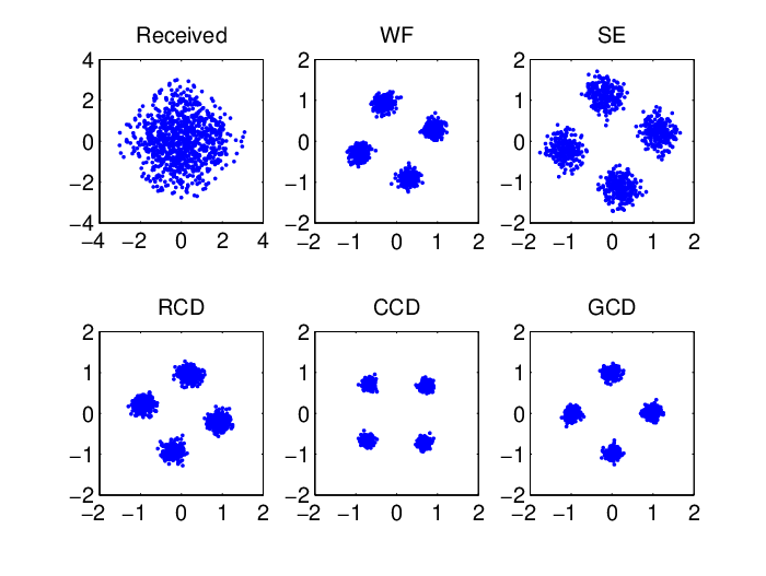
We investigate the application of the CD and WF methods to blind equalization in the presence of white Gaussian noise. The results of the super-exponential (SE) algorithm [48] are also included. The transmitted signal adopts quadrature PSK (QPSK) modulation, namely, $s(n)\in\{1,-1,{\rm j},-{\rm j}\}$. A typical FIR communication channel with impulse response $\{0.4,1,-0.7,0.6,0.3,-0.4,0.1\}$ is adopted [48]. Fig. 9 shows the constellations of the received signal and equalizer outputs of 1000 samples at SNR = 20 dB. We observe that the received signal is severely distorted due to the channel propagation. The SE, WF and CD methods succeed in recovering the transmitted signal up to a global phase rotation. We clearly see that the CCD and GCD have a higher recovery accuracy. Fig. 10 plots the ISI versus the number of iterations/cycles at SNR = 25 dB with 2000 samples. The ISI is averaged over 100 independent trials. In addition to faster convergence than the WF, WFOS, and SE, the CDs (especially CCD) arrive at a lower ISI. This means that the CDs also achieve a more accurate recovery.

Fig. 9: Scatter plots of constellations of received signal and equalizer outputs.

Fig. 10: ISI versus number of iterations/cycles.

VII Conclusion

This paper designs CD algorithms for efficiently solving the quartic polynomial minimization in phase retrieval. One appealing characteristic of our scheme is the conceptual and computational simplicity: the minimum of each one-dimensional coordinate optimization is obtained by root finding of a univariate cubic equation, which has a closed-form solution. Three different rules for coordinate selection yield three CD variants, namely, CCD, RCD, and GCD. The GCD selecting the coordinate associated with the largest absolute partial derivative converges faster than the cyclic and randomized CDs. Theoretically, we prove that the three CD algorithms converge to a stationary point for any initial value. We also prove that the RCD converges to the global minimum and achieves exact recovery with high probability provided that the sample size is large enough. The main advantage of the CD over the full gradient methods such as WF and WFOS is its faster convergence speed. The CD is also extended to solving the $\ell_{1}$-regularized quartic minimization for phase retrieval of sparse signals. In the new application to blind equalization, the CD can achieve lower ISI and higher recovery accuracy than several existing methods.

References

- [1] W.-J. Zeng and H. C. So, “Phase retrieval using coordinate decent techniques,” filed with U.S. Patent Office (No. 15/344,279), Nov. 2016.
- [2] E. J. Candès, Y. C. Eldar, T. Strohmer, and V. Voroninski, “Phase retrieval via matrix completion,” SIAM Rev., vol. 57, no. 2, pp. 225–251, 2015.
- [3] Y. Shechtman, Y. C. Eldar, O. Cohen, H. N. Chapman, J. Miao and M. Segev, “Phase retrieval with application to optical imaging,” IEEE Signal Process. Mag., vol. 32, no. 3, pp. 87–109, May 2015.
- [4] R. P. Millane, “Phase retrieval in crystallography and optics,” J. Opt. Soc. Amer. A., vol. 7, no. 3, pp. 394–411, Mar. 1990.
- [5] J. Miao, T. Ishikawa, Q. Shen, and T. Earnest, “Extending X-ray crystallography to allow the imaging of noncrystalline materials, cells, and single protein complexes,” Annu. Rev. Phys. Chem., vol. 59, pp. 387–410, 2008.
- [6] B. E. Allman, P. J. McMahon, K. A. Nugent, D. Paganin, D. Jacobson, M. Arif, and S. A. Werner, “Imaging: Phase radiography with neutrons,” Nature, vol. 408, no. 6809, pp. 158–159, 2000.
- [7] B. Baykal, “Blind channel estimation via combining autocorrelation and blind phase estimation,” IEEE Transactions on Circuits and Systems I, vol. 51, no. 6, pp. 1125–1131, Jun. 2004.
- [8] J. C. Dainty and J. R. Fienup, “Phase retrieval and image reconstruction for astronomy,” in Image Recovery: Theory and Application, H. Stark, Ed., San Diego, CA: Academic Press, pp. 231–275, 1987.
- [9] M. Stefik, “Inferring DNA structures from segmentation data,” Artificial Intelligence, vol. 11, no. 1, pp. 85–114, Aug. 1978.
- [10] R. Balan, P. Casazza, and D. Edidin, “On signal reconstruction without phase,” Appl. Comput. Harmon. Anal., vol. 20, no. 3, pp. 345–356, 2006.
- [11] K. Jaganathan, Y. C. Eldar and B. Hassibi, “STFT phase retrieval: Uniqueness guarantees and recovery algorithms,” IEEE J. Sel. Top. Signal Process., vol. 10, no. 4, pp. 770–781, Jun. 2016.
- [12] E. J. Candès, X. Li, and M. Soltanolkotabi, “Phase retrieval from coded diffraction patterns,” Appl. Comput. Harmon. Anal., vol. 39, no. 2, pp. 277–299, 2015.
- [13] E. J. Candès, X. Li, and M. Soltanolkotabi, “Phase retrieval via Wirtinger flow: Theory and algorithms,” IEEE Trans. Inf. Theory, vol. 61, no. 4, pp. 1985–2007, Apr. 2015.
- [14] E. J. Candès, T. Strohmer, and V. Voroninski, “PhaseLift: Exact and stable signal recovery from magnitude measurements via convex programming,” Commun. Pure Appl. Math., vol. 66, no. 8, pp. 1241–1274, 2013.
- [15] J. Sun, Q. Qu, and J. Wright, “A geometrical analysis of phase retrieval,” submitted to Found. Comput. Math., 2016. Online Available: http://arxiv.org/abs/1602.06664.
- [16] R. Gerchberg and W. Saxton, “A practical algorithm for the determination of phase from image and diffraction plane pictures,” Optik, vol. 35, pp. 237–246, 1972.
- [17] J. R. Fienup, “Phase retrieval algorithms: A comparison,” Appl. Opt., vol. 21, no. 15, pp. 2758–2769, 1982.
- [18] P. Netrapalli, P. Jain, and S. Sanghavi, “Phase retrieval using alternating minimization,” IEEE Trans. Signal Process., vol. 63, no. 18, pp. 4814–4826, Sep. 2015.
- [19] H. H. Bauschke, P. L. Combettes, and D. R. Luke, “Hybrid projection–reflection method for phase retrieval,” J. Opt. Soc. Amer. A, vol. 20, no. 6, pp. 1025–1034, 2003.
- [20] V. Elser, “Phase retrieval by iterated projections,” J. Opt. Soc. Amer. A, vol. 20, no. 1, pp. 40–55, 2003.
- [21] K. G. Murty and S. N. Kabadi, “Some NP-complete problems in quadratic and nonlinear programming,” Math. Program., vol. 39, no. 2, pp. 117–129, 1987.
- [22] Y. Chen and E. J. Candès, “Solving random quadratic systems of equations is nearly as easy as solving linear systems,” Neural Information Processing Systems, pp. 739–747, Dec. 2015, Montreal, Canada.
- [23] I. Waldspurger, A. d’Aspremont, and S. Mallat, “Phase recovery, MaxCut and complex semidefinite programming,” Math. Program., Ser. A, vol. 149, no. 1, pp. 47–81, Feb. 2015.
- [24] M. X. Goemans and D. P. Williamson, “Improved approximation algorithms for maximum cut and satisfiability problems using semidefinite programming,” J. ACM, vol. 42, no. 6, pp. 1115–1145, Nov. 1995.
- [25] Z.-Q. Luo, W.-K. Ma, A. M.-C. So, Y. Ye, and S. Zhang, “Semidefinite relaxation of quadratic optimization problems,” IEEE Signal Process. Mag., vol. 27, no. 3, pp. 20–34, May 2010.
- [26] X. Jiang and X. Liu, “Wirtinger flow method with optimal stepsize for phase retrieval,” IEEE Signal Process. Lett.,, vol. 23, no. 11, pp. 1627–1631, Nov. 2016.
- [27] E. J. Candès and M. Wakin, “An introduction to compressive sampling,” IEEE Signal Proces. Mag., vol. 25, no. 2, pp. 21–30, Mar. 2008.
- [28] E. J. Candès and T. Tao, “Near-optimal signal recovery from random projections: Universal encoding strategies,” IEEE Trans. Inf. Theory, vol. 52, no. 12, pp. 5406–5425, Dec. 2006.
- [29] S. Mukherjee and C. S. Seelamantula, “Fienup algorithm with sparsity constraints: Application to frequency-domain optical-coherence tomography,” IEEE Trans. Signal Process., vol. 62, no. 18, pp. 4659–4672, Sep. 2014.
- [30] T. Cai, X. Li, and Z. Ma, “Optimal rates of convergence for noisy sparse phase retrieval via thresholded Wirtinger flow,” Ann. Stat., vol. 44, no. 5, pp. 2221–2251, Oct. 2016.
- [31] J. A. Tropp and A. C. Gilbert, “Signal recovery from random measurements via orthogonal matching pursuit,” IEEE Trans. Inf. Theory, vol. 53, no. 12, pp. 4655–4666, Dec. 2007.
- [32] W.-J. Zeng, H. C. So, and X. Jiang, “Outlier-robust greedy pursuit algorithms in -space for sparse approximation,” IEEE Trans. Signal Process., vol. 64, no. 1, pp. 60–75, Jan. 2016.
- [33] Y. Shechtman, A. Beck, and Y. C. Eldar, “GESPAR: Efficient phase retrieval of sparse signals,” IEEE Trans. Signal Process., vol. 62, no. 4, pp. 928–938, Feb. 2014.
- [34] S. J. Wright, “Coordinate descent algorithms,” Math. Program., Ser. A, vol. 151, no. 1, pp. 3–34, Jun. 2015.
- [35] Y. Nesterov, “Efficiency of coordinate-descent methods on huge-scale optimization problems,” SIAM J. Optim., vol. 22, no. 2, pp. 341–362, 2012.
- [36] A. Greenbaum, Iterative Methods for Solving Linear Systems. SIAM, Philadelphia, PA, 1997.
- [37] D. G. Luenberger and Y. Ye, Linear and Nonlinear Programming. Springer, New York, 2016.
- [38] E. T. Whittaker and G. Robinson, “The solution of the cubic”, Section 62, The Calculus of Observations: A Treatise on Numerical Mathematics, 4th ed. New York: Dover, pp. 124–126, 1967.
- [39] A. Beck and L. Tetruashvili, “On the convergence of block coordinate descent type methods,” SIAM J. Optim., vol. 23, no. 4, pp. 2037–2060, 2013.
- [40] H. L. Royden, Real Analysis. Macmillan Publishing Company, NY, 1988.
- [41] D. Bertsekas, Nonlinear Programming. Athena Scientific, Belmont, 1999.
- [42] D. R. Luke, J. V. Burke, and R. G. Lyon, “Optical wavefront reconstruction: Theory and numerical methods,” SIAM Rev., vol. 44, no. 2, pp. 169–224, 2002.
- [43] R. Tibshirani, “Regression shrinkage and selection via the LASSO,” J. R. Staist. Soc. Ser. B (Methodol.), vol. 58, no. 1, pp. 267–288, 1996.
- [44] S. S. Chen, D. L. Donoho, and M. A. Saunders, “Atomic decomposition by basis pursuit,” SIAM Rev., vol. 43, no. 1, pp. 129–159, 2001.
- [45] S. J. Wright, R. D. Nowak, and M. Figueiredo, “Sparse reconstruction by separable approximation,” IEEE Trans. Signal Process., vol. 57, no. 7, pp. 2479–2493, Jul. 2009.
- [46] C. R. Johnson, Jr., P. Schniter, T. J. Endres, J. D. Behm, D. R. Brown, and R. A. Casas, “Blind equalization using the constant modulus criterion: A review,” Proc. IEEE, vol. 86, no. 10, pp. 1927–1950, Oct. 1998.
- [47] D. N. Godard, “Self-recovering equalization and carrier tracking in two-dimensional data communication systems,” IEEE Trans. Commun., vol. 28, pp. 1867–1875, Nov. 1980.
- [48] O. Shalvi and E. Weinstein, “Super-exponential method for blind deconvolution,” IEEE Trans. Inf. Theory, vol. 39, no. 2, pp. 504–519, Mar. 1993.