Wave propagation and homogenization in 2D and 3D lattices: a semi-analytical approach

Abstract

Wave motion in two- and three-dimensional periodic lattices of beam members supporting longitudinal and flexural waves is considered. An analytic method for solving the Bloch wave spectrum is developed, characterized by a generalized eigenvalue equation obtained by enforcing the Floquet condition. The dynamic stiffness matrix is shown to be explicitly Hermitian and to admit positive eigenvalues. Lattices with hexagonal, rectangular, tetrahedral and cubic unit cells are analyzed. The semi-analytical method can be asymptotically expanded for low frequency yielding explicit forms for the Christoffel matrix describing wave motion in the quasistatic limit.

1 Introduction

Two- and three-dimensional lattices of connected beams can provide pentamode-like behavior in the static limit [1, 2]. One reason for interest in such structures is that they exhibit one-wave behaviour characteristic of scalar or acoustic wave systems, while also displaying material anisotropy, so that anisotropic acoustic effects are possible. Such scalar dynamic effective properties are perhaps surprising since periodic lattice structures support multiple wave types yielding complex dispersion properties described by Bloch-Floquet spectra, particularly band gaps [3, 4] and anisotropic propagation [5]. At the same time, the relatively simple geometry of two- and three-dimensional lattices allows for the possibility of mechanical simplifications that maintain the underlying structural dynamics of the continuous beam elements while leading to accurate predictions for the dispersion properties. This paper focuses on the latter aspect, as we develop a semi-analytical formalism that reduces the Bloch wave problem to an analytically simple form while retaining the crucial mechanics of the structure.

Two distinct approaches [6] to analysing waves in periodic structures can be distinguished based on the number of degrees of freedom: finite models and infinite models. The former naturally includes the finite elements method (FEM) for which strategies have been developed that are specifically designed to treat lattice structures. Thus, [4] developed a FEM procedure for calculating dispersion curves of hexagonal, square and triangular lattice structures. FEM has been used by [5] to consider waves in regular and re-entrant hexagonal lattices and by [7] to examine hexagonal chiral lattices as phononic crystals. Infinite methods, as in this paper, retain some of the characteristics of the continuous nature of the structure at the smallest scale. A simple beam considered as a separate entity displays an infinite number of modes; it is therefore no surprise that a model based on such elements has an infinite number of Bloch-Floquet branches.

The fundamental step in deriving the dispersion relation for waves in a periodic structure is the application of the Floquet condition on the unit cell of the lattice. Whatever approach is used, whether FEM or semi-analytical, this step reduces the problem to a generalized eigenvalue problem for the system (or stiffness) matrix. The main distinction between finite and infinite models is that the former reduce to linear systems with eigenvalue equal to the square of the frequency, whereas infinite models necessarily involve finding roots of transcendental equations. There are, however, computational approaches adapted to this problem, such as that of Wittrick and Williams [6] based on Householder’s algorithm.

Regarding other infinite methods for solving dynamic waves problems in lattices, we note that an interesting alternative wave-based approach for determining the Bloch waves in 2D periodic structures was proposed by [8]. The semi-analytical method considers the explicit waves propagating back and forth on each member, coupled by reflection and transmission matrices at joints. The present method is similar to that of [8] in that both approaches yield exact dispersion relations within the context of the beam theories employed (Timoshenko beam theory was used in [8]). However, the present approach is arguably simpler in that it does not require propagation and reflection/transmission matrices for the multiple wave types. Instead, the crucial ingredient in the present method is the dynamic stiffness matrix that relates forces at the two ends of a beam member to the displacements at either end.

An important limit of any dynamic model is the low frequency, quasistatic or homogenization limit. Although static homogenization theory for quite general lattice structures has been developed by several authors, e.g. [9, 10], these approaches do not derive the homogenized properties from the limit of a dynamic model. An exception is the paper by [11] who showed for a triangular lattice that only by including the flexural wave effects is the effective mass properly modeled in the low frequency limit. Simpler beam models which ignore flexural waves, or bending, show quasistatic wave speeds with effective mass that is less than the total mass of the unit cell [11]. This suggests that models ignoring flexural effects do not properly account for the distributed mass on the wave-bearing segments of the structure, and cannot yield the correct quasistatic results.

The analytical approach used here represents the lattice members as uni-dimensional beams supporting longitudinal and flexural waves. A strategy for implementing this was outlined by [3] who introduced the necessary stiffness matrix relating forces and displacements at the ends of a beam. By combining these matrices it is possible to represent any periodic lattice, in principle. The method of [3] was used in [11] to consider lattices with triangular unit cell structure, and for square cell lattices in [12]. In this paper we develop further the approach proposed by [3] and [11]. We present, for the first time, analysis of a general hexagonal unit cell lattice, a structure of great interest in relation to graphene and other phenomena. Also, the method is extended into 3D to analyze the tetrahedral unit cell lattice. The formulation is semi-analytical to the extent that all matrix elements are explicit, the dispersion relation for square and cubic lattices are derived analytically. Although one could obtain analytic dispersion relations for hexagonal and tetrahedral lattices using symbolic computation [13], direct numerical methods are employed at the final stage to perform computation. The semi-analytical nature of the solution allows us to extract the low frequency asymptotics, and to find closed-form expressions for the quasistatic Christoffel matrix, as demonstrated for hexagonal and rectangular unit cell lattices in 2D. In this sense the present study is step in the continuation from low frequency (quasi-static) response governed by effective elastic stiffness and density to dynamic effective medium models.

The present analysis does not include torsion in the individual members. The beams are assumed to have large length to thickness ratio, and hence a static applied macroscopic torsion is borne at the level of the unit cell by flexure of the members. Bending is the dominant effect for producing torsion in the lattice structures considered here. This can be seen a posteriori from the comparisons below with full elastodynamic simulations which do not display Bloch-Floquet branches with significant torsional effects at level of the lattice member. In other words, torsion in individual members is ignored because we are only including the dynamic counterparts of the micro-effects that lead to the static effective medium. Note that the present model allows for rigid body rotation at the unit cell level, which is consistent with static homogenization [2].

The format of the paper is as follows. The solution method for hexagonal and tetrahedral lattices is summarized in §2, where the Bloch wave condition is explicitly used to derive the dispersion relation for Floquet modes. The detailed derivation of the system matrix for the hexagonal lattice is presented in §3. The low frequency asymptotics are examined in §4 where the explicit form of the quasi-static Christoffel matrix is derived. The dynamic and quasi-static solutions are obtained for the rectangular lattice in §5, and for cubic lattice in §6. In addition, numerical examples in §5 and §6 compare results from the present theory with fully elastodynamic FEM computations for hexagonal, rectangular, tetrahedral and cubic lattices.

2 Dispersion relation

2.1 Structures and structural parameters

We focus our attention on two example structures in 2D and 3D, hexagonal and tetrahedral lattices, respectively. Each may be defined by two points ${\bf a}_{1}$, ${\bf a}_{2}$ inside the unit cell ${\mathscr{P}}$ spanned by vectors ${\bf e}_{1}$, ${\bf e}_{2}$ (and ${\bf e}_{3}$ in 3D), see Fig. 1. The unit cell ${\mathscr{P}}$ is then periodically translated to cover the whole plane (space in 3D) and thereby make the infinitely extended lattice. We assume that all material parameters are periodic such that the properties in any translated cell ${\mathscr{P}}+n{\bf e}_{1}+m{\bf e}_{2}\ \ (+l{\bf e}_{3}\ \ {\text{in 3D}})$ coincide with those in ${\mathscr{P}}$.

Every point ${\bf a}_{i}$ in the lattice is connected to three (four in 3D) neighboring points ${\bf a}_{j}$ by rods $[{\bf a}_{i},{\bf a}_{j}]$ with length $l_{ij}=|{\bf a}_{i}-{\bf a}_{j}|$ and direction ${\bf e}_{ij}=l_{ij}^{-1}({\bf a}_{i}-{\bf a}_{j})$. There are masses $m_{1}$, $m_{2}$ with moments of inertia $I_{1}$, $I_{2}$ at the points ${\bf a}_{1}$, ${\bf a}_{2}$. The rod $[{\bf a}_{i},{\bf a}_{j}]$ has axial stiffness $\mu_{ij}$, beam flexural coefficient $\lambda_{ij}$ and lineal density $\rho_{ij}$ (these are related to the rod Young’s modulus $E_{ij}$, cross-sectional area $A_{ij}$, radius of gyration $\kappa_{ij}$ and volumetric density $\rho_{ij}^{V}$ by $\mu_{ij}=E_{ij}A_{ij}$, $\lambda_{ij}=E_{ij}A_{ij}\kappa_{ij}^{2}$, $\rho_{ij}=\rho_{ij}^{V}A_{ij}$).

Figure 1: The hexagonal (honeycomb) lattice

₂ a₁

Figure 2: The tetrahedral lattice

2.2 Analytic dispersion relation

Considering the rod ${\bf e}_{ij}$, let ${\bf u}_{i}$, ${\bf u}_{j}$ denote the displacement at the end points ${\bf a}_{i}$, ${\bf a}_{j}$, respectively. Let ${\bf f}_{ij}$ denote the force at point ${\bf a}_{i}$ from the rod ${\bf e}_{ij}$. The precise form of the displacement and force 3-vectors (6-vectors for 3D case) will be defined in Section 3, for the moment we do not need to know their specific nature, except to note that they include both longitudinal and flexural effects. The equilibrium equation at point ${\bf a}_{i}$ is then

$$\sum\limits_{j\in\mathcal{N}_{i}}{\bf f}_{ij}=-\omega^{2}{\bf M}_{i}{\bf u}_{i},\quad{\bf M}_{i}=\mathrm{diag}(m_{i},m_{i},I_{i})\ \ \text{in 2D or }\mathrm{diag}(m_{i},m_{i},m_{i},I_{i},I_{i},I_{i})\ \ \text{in 3D},$$ (1)

where ${\mathcal{N}}_{i}$ is the set of points connected with ${\bf a}_{i}$. It is notable that this approach allows concentrated masses at the junctions which are included in the matrix ${\bf M}_{i}$. The force ${\bf f}_{ij}$ may be expressed in terms of the end point displacements

$${\bf f}_{ij}={\bf P}_{ij}^{(2)}{\bf u}_{j}-{\bf P}_{ij}^{(1)}{\bf u}_{i},$$ (2)

where the frequency dependent stiffness matrices ${\bf P}_{ij}^{(1)}(\omega)$, ${\bf P}_{ij}^{(2)}(\omega)$ are derived in Section 3.

Applying the Floquet periodic conditions

$${\bf u}_{j} =\exp(i{\bf k}\cdot{\bf g}_{j}){\bf u}_{1},\ \ {\bf g}_{j}={\bf a}_{j}-{\bf a}_{1},\ \ j\in{\mathcal{N}}_{2},$$ (3)

$${\bf u}_{j} =\exp(i{\bf k}\cdot{\bf g}_{j}){\bf u}_{2},\ \ {\bf g}_{j}={\bf a}_{j}-{\bf a}_{2},\ \ j\in{\mathcal{N}}_{1}$$

and using eqs. (1) and (2) leads to

$$\sum\limits_{j\in\mathcal{N}_{1}}\big({\bf P}_{1j}^{(2)}\exp(i{\bf k}\cdot{\bf g}_{j})\,{\bf u}_{2}-{\bf P}_{1j}^{(1)}{\bf u}_{1}\big) =-\omega^{2}{\bf M}_{1}{\bf u}_{1},$$ (4)

$$\sum\limits_{j\in\mathcal{N}_{2}}\big({\bf P}_{2j}^{(2)}\exp(i{\bf k}\cdot{\bf g}_{j})\,{\bf u}_{1}-{\bf P}_{2j}^{(1)}{\bf u}_{2}\big) =-\omega^{2}{\bf M}_{2}{\bf u}_{2}.$$

For each $j\in\mathcal{N}_{2}$ there is a unique $\bar{j}\in\mathcal{N}_{1}$ such that

$${\bf P}_{2j}^{(2)}e^{i{\bf k}\cdot{\bf g}_{j}}=\Big({\bf P}_{1\bar{j}}^{(2)}e^{i{\bf k}\cdot{\bf g}_{\bar{j}}}\Big)^{+},\ \ {\bf P}_{2j}^{(1)}={\bf P}_{1\bar{j}}^{(3)},\ \$$ (5)

where $+$ denotes the Hermitian conjugation and the matrices ${\bf P}_{1j}^{(3)}$ are defined in Section 3. Hence it is possible to express the second equation of (4) in terms of a sum over neighboring links of ${\bf a}_{1}$. Introducing matrices

$${\bf H}_{1}=\sum\limits_{j\in\mathcal{N}_{1}}{\bf P}_{1j}^{(1)},\ \ {\bf H}_{2}=-\sum\limits_{j\in\mathcal{N}_{1}}{\bf P}_{1j}^{(2)}\exp(i{\bf k}\cdot{\bf g}_{j}),\ \ {\bf H}_{3}=\sum\limits_{j\in\mathcal{N}_{1}}{\bf P}_{1j}^{(3)}$$ (6)

equations (4) can then be rewritten in the form

$${\bf H}{\bf u}=\omega^{2}{\bf M}{\bf u}$$ (7)

with

$${\bf u}=\begin{pmatrix}{\bf u}_{1}\\ {\bf u}_{2}\end{pmatrix},\ \ {\bf M}=\mathrm{diag}({\bf M}_{1},{\bf M}_{2}),\ \ {\bf H}\equiv{\bf H}(\omega,{\bf k})=\begin{pmatrix}{\bf H}_{1}&{\bf H}_{2}\\ {\bf H}_{2}^{+}&{\bf H}_{3}\end{pmatrix}\ \ \big(={\bf H}^{+}\big).$$ (8)

Then Floquet curves (dispersion curves) $\omega_{n}({\bf k})$ can be found from the equation

$$\det({\bf H}(\omega,{\bf k})-\omega^{2}{\bf M})=0.$$ (9)

Note that according to Section 3 (see eqs. (6), (27), (19) and (24)), the matrices ${\bf H}_{1}$ and ${\bf H}_{3}$ are real symmetric, so that the matrix ${\bf H}$ is Hermitian, in turn guaranteeing that the dispersion relation (9) is real valued for real $\omega$, ${\bf k}$. We will return to this equation in Section 3 after we have described the displacements and forces, and derived the stiffness matrices.

3 Dynamic stiffness matrices

3.1 Longitudinal wave equation

Consider the rod ${\bf e}_{ij}$ with uniform Young’s modulus $\mu_{ij}$ and density $\rho_{ij}$. Let $u_{ij}(x)$ denote the component of the displacement in the ${\bf e}_{ij}-$direction at any point $x$ (a one-dimensional linear coordinate parameter) of $[{\bf a}_{i},{\bf a}_{j}]$. The displacement $u_{ij}$ satisfies the wave equation for longitudinal wave motion and its associated boundary conditions (BCs)

$$\mu_{ij}\frac{\partial^{2}}{\partial x^{2}}u_{ij}=-\omega^{2}\rho_{ij}u_{ij},\ \ u_{ij}(0)={\bf e}_{ij}\cdot{\bf u}_{i},\ \ u_{ij}(l_{ij})={\bf e}_{ij}\cdot{\bf u}_{j}.$$ (10)

Solving (10),

$$u_{ij}(x)=\frac{{\bf e}_{ij}\cdot{\bf u}_{i}\sin(s_{ij}\omega(l_{ij}-x))+{\bf e}_{ij}\cdot{\bf u}_{j}\sin(s_{ij}\omega x)}{\sin(s_{ij}\omega l_{ij})},\ \ s_{ij}=\sqrt{\frac{\rho_{ij}}{\mu_{ij}}},$$ (11)

implying that the longitudinal force ${\bf f}_{ij}$ acting on the point ${\bf a}_{i}$ is

$${\bf f}_{ij\ wave}\equiv\mu_{ij}\frac{\partial u_{ij}}{\partial x}(0)\,{\bf e}_{ij}=\frac{\mu_{ij}s_{ij}\omega}{\sin(s_{ij}\omega l_{ij})}\,{\bf e}_{ij}{\bf e}_{ij}^{T}\big({\bf u}_{j}-{\bf u}_{i}\cos(s_{ij}\omega l_{ij})\big).$$ (12)

3.2 Flexural wave equation

The kinematic BCs for flexural wave motion involve both the flexural displacement and the non-torsional rotation at the ends of the rod. In 2D, define the unit vector perpendicular to the plane of the lattice, ${\bf e}_{b}={\bf e}_{1}\wedge{\bf e}_{2}/|{\bf e}_{1}\wedge{\bf e}_{2}|$. The flexural displacement $v_{ij}(x)$ at any point $x$ on the rod ${\bf e}_{ij}$ is then defined as the component of the displacement in the ${\bf e}_{ij}^{\perp}-$ direction, where

$${\bf e}_{ij}^{\perp}={{\bf e}_{b}\wedge{\bf e}_{ij}}.$$ (13)

The generalized 2D displacement vectors are therefore “three-dimensional” with two components for the longitudinal motion and one for flexural. The flexural wave equation and its BCs are, with $v^{\prime}=\partial v/\partial x$,

$$-\lambda_{ij}\frac{\partial^{4}v_{ij}}{\partial x^{4}}=-\omega^{2}\rho_{ij}v_{ij},\quad$$ (14)

$$v_{ij}(0)={\bf e}_{ij}^{\perp}\cdot{\bf u}_{i},\ \ v_{ij}(l_{ij})={\bf e}_{ij}^{\perp}\cdot{\bf u}_{j},\ \ v_{ij}^{\prime}(0)={\bf e}_{b}\cdot{\bf u}_{i},\ \ v_{ij}^{\prime}(l_{ij})={\bf e}_{b}\cdot{\bf u}_{j}.$$

The generalized force (shear force and bending moment) at point ${\bf a}_{i}$ due to bending is

$${\bf f}_{ij\ bending}=-\lambda_{ij}\frac{\partial^{3}v_{ij}}{\partial x^{3}}{\bf e}_{ij}^{\perp}+\lambda_{ij}\frac{\partial^{2}v_{ij}}{\partial x^{2}}{\bf e}_{b}.$$ (15)

In 3D we extend the definition of the end point flexural displacement by defining two non-torsional rotation components in the directions ${\bf e}_{b}$ and ${\bf e}_{b}^{\prime}$, and the related shear force components along ${\bf e}_{ij}^{\perp}$ and ${\bf e}_{ij}^{\perp\prime}$, where

$${\bf e}_{ij}^{\perp}=({\bf r},{\bf 0}_{3}),\ \ {\bf e}_{b}=({\bf 0}_{3},{\bf e}_{ij}\wedge{\bf r}),\ \ {\bf e}_{ij}^{\perp\prime}=({\bf e}_{ij}\wedge{\bf r},{\bf 0}_{3}),\ \ {\bf e}_{b}^{\prime}=-({\bf 0}_{3},{\bf r}).$$ (16)

Here ${\bf 0}_{3}$ is 3D zero-vector, ${\bf r}={\bf e}_{\alpha}\wedge{\bf e}_{ij}/|{\bf e}_{\alpha}\wedge{\bf e}_{ij}|$ and ${\bf e}_{\alpha}$ is some (any) vector ${\bf e}_{1}$ or ${\bf e}_{2}$ or ${\bf e}_{3}$ whichever is not parallel to ${\bf e}_{ij}$. Let $w_{ij}(x)$ denote the displacement in direction ${\bf e}_{ij}^{\perp\prime}$, $w_{ij}^{\prime}=\partial w_{ij}/\partial x$, then the flexural wave equation and its BCs for the extra dimension in 3D case can be written as eq. (14) combined with

$$-\lambda_{ij}\frac{\partial^{4}w_{ij}}{\partial x^{4}}=-\omega^{2}\rho_{ij}w_{ij},\quad$$ (17)

$$w_{ij}(0)={\bf e}_{ij}^{\perp\prime}\cdot{\bf u}_{i},\ \ w_{ij}(l_{ij})={\bf e}_{ij}^{\perp\prime}\cdot{\bf u}_{j},\ \ w_{ij}^{\prime}(0)={\bf e}_{b}^{\prime}\cdot{\bf u}_{i},\ \ w_{ij}^{\prime}(l_{ij})={\bf e}_{b}^{\prime}\cdot{\bf u}_{j}.$$

The additional generalized force term at point ${\bf a}_{i}$ is

$${\bf f}^{\prime}_{ij\ bending}=-\lambda_{ij}\frac{\partial^{3}w_{ij}}{\partial x^{3}}{\bf e}_{ij}^{\perp\prime}+\lambda_{ij}\frac{\partial^{2}w_{ij}}{\partial x^{2}}{\bf e}_{b}^{\prime}.$$ (18)

In summary, the components of ${\bf u}_{i}$ in the ${\bf e}_{ij}^{\perp}$, ${\bf e}_{ij}^{\perp\prime}$ and ${\bf e}_{b}$, ${\bf e}_{b}^{\prime}$ directions are the transverse deflection and beam rotation angle, respectively. The force components in direction ${\bf e}_{ij}^{\perp}$ and ${\bf e}_{ij}^{\perp\prime}$ are the resultant shear force while the ${\bf e}_{b}$ and ${\bf e}_{b}^{\prime}$ ”force” components represent the bending moment. Note that in 3D, there are three displacement components and three rotation components. In this way the coupled longitudinal and flexural dynamics of the 2D lattice are described in terms of ”three-dimensional”vectors for displacement and forces in 2D, and ”six-dimensional” vectors for 3D lattices.

The generalized forces at the two ends of the rod are related to the displacements there by the stiffness matrix ${\bf K}$, defined such that

$$\begin{pmatrix}{\bf e}_{ij}^{\perp}\cdot{\bf f}_{ij}\\ {\bf e}_{b}\cdot{\bf f}_{ij}\\ {\bf e}_{ij}^{\perp}\cdot{\bf f}_{ji}\\ {\bf e}_{b}\cdot{\bf f}_{ji}\end{pmatrix}=-\lambda_{ij}{\bf K}(\omega)\begin{pmatrix}{\bf e}_{ij}^{\perp}\cdot{\bf u}_{i}\\ {\bf e}_{b}\cdot{\bf u}_{i}\\ {\bf e}_{ij}^{\perp}\cdot{\bf u}_{j}\\ {\bf e}_{b}\cdot{\bf u}_{j}\end{pmatrix},\quad{\bf K}=\begin{pmatrix}{\bf K}_{1}&{\bf K}_{2}\\ {\bf K}_{2}^{T}&{\bf K}_{3}\end{pmatrix}.$$ (19)

The bending forces (15) and (18) at lattice site $i$ from rod $ij$ therefore becomes

$$\bf{\displaystyle f}_{ij\ bending}=-\lambda_{ij}\big({\bf e}_{ij}^{\perp},\,{\bf e}_{b}\big)\Big({\bf K}_{1}\big({\bf e}_{ij}^{\perp},\,{\bf e}_{b}\big)^{T}{\bf u}_{i}+{\bf K}_{2}\big({\bf e}_{ij}^{\perp},\,{\bf e}_{b}\big)^{T}{\bf u}_{j}\Big),$$ (20)

$$\bf{\displaystyle f}^{\prime}_{ij\ bending}=-\lambda_{ij}\big({\bf e}_{ij}^{\perp\prime},\,{\bf e}_{b}^{\prime}\big)\Big({\bf K}_{1}\big({\bf e}_{ij}^{\perp\prime},\,{\bf e}_{b}^{\prime}\big)^{T}{\bf u}_{i}+{\bf K}_{2}\big({\bf e}_{ij}^{\perp\prime},\,{\bf e}_{b}^{\prime}\big)^{T}{\bf u}_{j}\Big).$$

We next derive the explicit form of the stiffness matrix.

3.3 Solution of the flexural stiffness matrix

With eqs. (14) and (17) in mind, consider the solution to

$$\frac{\partial^{4}w}{\partial x^{4}}-\gamma^{4}w=0,\quad x\in[0,l],$$ (21)

in the form

$$w(x)=\frac{1}{2(1-cc_{h})}\big\{\big[(c-c_{h})(\cos\gamma x-\cosh\gamma x)+(s+s_{h})(\sin\gamma x-\sinh\gamma x)\big]w(l)$$

$$+\frac{1}{\gamma}\big[(s_{h}-s)(\cos\gamma x-\cosh\gamma x)+(c-c_{h})(\sin\gamma x-\sinh\gamma x)\big]w^{\prime}(l)$$

$$+\big[(1-cc_{h}+ss_{h})\cos\gamma x+(1-cc_{h}-ss_{h})\cosh\gamma x+(cs_{h}+sc_{h})(\sinh\gamma x-\sin\gamma x)\big]w(0)$$

$$+\frac{1}{\gamma}\big[(sc_{h}-cs_{h})(\cos\gamma x-\cosh\gamma x)+(1-cc_{h}-ss_{h})\sin\gamma x+(1-cc_{h}+ss_{h})\sinh\gamma x\big]w^{\prime}(0)\big\},$$ (22)

where $c=\cos\gamma l$, $s=\sin\gamma l$, $c_{h}=\cosh\gamma l$, $s_{h}=\sinh\gamma l$. $v(x)$ and $w(x)$ have the same form of solution, so that the stiffness matrix is the same. According to its definition in (19) the stiffness matrix ${\bf K}$ satisfies

$$\begin{pmatrix}w^{\prime\prime\prime}(0)\\ -w^{\prime\prime}(0)\\ -w^{\prime\prime\prime}(l)\\ w^{\prime\prime}(l)\end{pmatrix} ={\bf K}(\omega)\begin{pmatrix}w(0)\\ w^{\prime}(0)\\ w(l)\\ w^{\prime}(l)\end{pmatrix}.$$ (23)

The explicit form of the stiffness matrix then follows from (22) as

$${\bf K}(\omega)=\frac{\gamma^{2}}{1-cc_{h}}\begin{pmatrix}\gamma(cs_{h}+sc_{h})&ss_{h}&-\gamma(s+s_{h})&c_{h}-c\\ ss_{h}&\gamma^{-1}(sc_{h}-cs_{h})&c-c_{h}&\gamma^{-1}(s_{h}-s)\\ -\gamma(s+s_{h})&c-c_{h}&\gamma(cs_{h}+sc_{h})&-ss_{h}\\ c_{h}-c&\gamma^{-1}(s_{h}-s)&-ss_{h}&\gamma^{-1}(sc_{h}-cs_{h})\end{pmatrix}.$$ (24)

3.4 Total force and stiffness matrices

The total force at point $i$ from rod ${\bf e}_{ij}$ now follows from (12) and (15),

$${\bf f}_{ij}={\bf f}_{ij\ wave}(0)+{\bf f}_{ij\ bending}(0)+{\bf f}^{\prime}_{ij\ bending}(0),$$ (25)

where ${\bf f}^{\prime}_{ij\ bending}(0)$ doesn’t exist in 2D case. Set

$$\tilde{\mu}_{ij}={\mu}_{ij}/l_{ij},\quad\tilde{s}_{ij}(\omega)=\omega s_{ij}l_{ij},\quad\gamma_{ij}(\omega)=\big(\omega^{2}\rho_{ij}/\lambda_{ij}\big)^{1/4},\quad{\bf A}_{ij}={\bf e}_{ij}{\bf e}_{ij}^{T},$$ (26)

The dynamic stiffness matrices introduced in eqs. (2) and (5) then follow from (12), (20) and (25) as

$${\bf P}_{ij}^{(1)} =\tilde{\mu}_{ij}\tilde{s}_{ij}\cot\tilde{s}_{ij}{\bf A}_{ij}+\lambda_{ij}\big({\bf e}_{ij}^{\perp},\,{\bf e}_{b}\big){\bf K}_{1}\big({\bf e}_{ij}^{\perp},\,{\bf e}_{b}\big)^{T}+\lambda_{ij}\big({\bf e}_{ij}^{\perp\prime},\,{\bf e}_{b}^{\prime}\big){\bf K}_{1}\big({\bf e}_{ij}^{\perp\prime},\,{\bf e}_{b}^{\prime}\big)^{T},$$

$${\bf P}_{ij}^{(2)} =\tilde{\mu}_{ij}\tilde{s}_{ij}\csc\tilde{s}_{ij}{\bf A}_{ij}-\lambda_{ij}\big({\bf e}_{ij}^{\perp},\,{\bf e}_{b}\big){\bf K}_{2}\big({\bf e}_{ij}^{\perp},\,{\bf e}_{b}\big)^{T}-\lambda_{ij}\big({\bf e}_{ij}^{\perp\prime},\,{\bf e}_{b}^{\prime}\big){\bf K}_{2}\big({\bf e}_{ij}^{\perp\prime},\,{\bf e}_{b}^{\prime}\big)^{T},$$ (27)

$${\bf P}_{ij}^{(3)} =\tilde{\mu}_{ij}\tilde{s}_{ij}\cot\tilde{s}_{ij}{\bf A}_{ij}+\lambda_{ij}\big({\bf e}_{ij}^{\perp},\,{\bf e}_{b}\big){\bf K}_{3}\big({\bf e}_{ij}^{\perp},\,{\bf e}_{b}\big)^{T}+\lambda_{ij}\big({\bf e}_{ij}^{\perp\prime},\,{\bf e}_{b}^{\prime}\big){\bf K}_{3}\big({\bf e}_{ij}^{\perp\prime},\,{\bf e}_{b}^{\prime}\big)^{T}.$$

where ${\bf K}$ is defined by eq. (24) with

$$\gamma=\gamma_{ij},\ \ c=\cos\gamma_{ij}l_{ij},\ \ s=\sin\gamma_{ij}l_{ij},\ \ c_{h}=\cosh\gamma_{ij}l_{ij},\ \ s_{h}=\sinh\gamma_{ij}l_{ij}.$$ (28)

The identities (5) are a consequence of the relations ${\bf K}_{2}^{T}={\bf J}{\bf K}_{2}{\bf J}$, ${\bf K}_{3}={\bf J}{\bf K}_{1}{\bf J}$ where ${\bf J}=\mathrm{diag}(1,-1)$. The force ${\bf f}_{ij}$ at point ${\bf a}_{i}$ given by eq. (2) then follows from (12), (20) and (25).

4 Effective wave speeds at low frequency

4.1 Low frequency asymptotics

The low-frequency asymptotic behavior of ${\bf K}$ defined in (24) is, using ${\bf K}_{3}={\bf J}{\bf K}_{1}{\bf J}$,

$${\bf K}_{1} =l^{-2}\begin{pmatrix}{12}\,l^{-1}&6\\ 6&{4}\,{l}\end{pmatrix}+\frac{\gamma^{4}l^{2}}{35}\begin{pmatrix}-13\,l^{-1}&-\frac{11}{6}\\ -\frac{11}{6}&-\frac{l}{3}\end{pmatrix}+\text{O}(\gamma^{8}),$$ (29)

$${\bf K}_{2} =l^{-2}\begin{pmatrix}-{12}\,l^{-1}&6\\ -6&2\,l\end{pmatrix}+\frac{\gamma^{4}l^{2}}{70}\begin{pmatrix}-9\,l^{-1}&\frac{13}{6}\\ -\frac{13}{6}&\frac{l}{2}\end{pmatrix}+\text{O}(\gamma^{8}),$$

implying that ${\bf K}(0)$ is positive semi-definite having eigenvalues $30$ and $2$ with non-normalized eigenvectors $(2,1,-2,1)^{T}$ and $(0,1,0,-1)^{T}$, respectively. The null vectors of ${\bf K}(0)$, $(1,0,1,0)^{T}$ and $(-l,2,l,2)^{T}$, correspond to rigid body displacement and rotation, respectively.

The low frequency expansions of the dynamic stiffness matrices of eq. (27) are

$${\bf P}_{ij}^{\big(\stackrel{{\scriptstyle 1}}{{3}}\big)}(\omega)= \tilde{\mu}_{ij}{\bf A}_{ij}+2\lambda_{ij}l_{ij}^{-3}\Big(6({\bf A}_{ij}^{\perp}+{\bf A}_{ij}^{\perp\prime})\pm 3({\bf A}_{ij}^{b\perp}+{\bf A}_{ij}^{b\perp\prime}+{\bf A}_{ij}^{\perp b}+{\bf A}_{ij}^{\perp b\prime})l_{ij}+2({\bf A}_{b}+{\bf A}_{b}^{\prime})l_{ij}^{2}\Big)$$ (30)

$$-\frac{1}{3}\omega^{2}\rho_{ij}l_{ij}\Big({\bf A}_{ij}+\frac{1}{70}\big(78({\bf A}_{ij}^{\perp}+{\bf A}_{ij}^{\perp\prime})\pm 11({\bf A}_{ij}^{\perp b}+{\bf A}_{ij}^{\perp b\prime}+{\bf A}_{ij}^{b\perp}+{\bf A}_{ij}^{b\perp\prime})l_{ij}$$

$$+2({\bf A}_{b}+{\bf A}_{b}^{\prime})l_{ij}^{2}\big)\Big)+\text{O}(\omega^{4}),$$

$${\bf P}_{ij}^{(2)}(\omega)= \tilde{\mu}_{ij}{\bf A}_{ij}+2\lambda_{ij}l_{ij}^{-3}\Big(6({\bf A}_{ij}^{\perp}+{\bf A}_{ij}^{\perp\prime})+3({\bf A}_{ij}^{b\perp}+{\bf A}_{ij}^{b\perp\prime}-{\bf A}_{ij}^{\perp b}-{\bf A}_{ij}^{\perp b\prime})l_{ij}-({\bf A}_{b}+{\bf A}_{b}^{\prime})l_{ij}^{2}\Big)$$

$$+\frac{1}{6}\omega^{2}\rho_{ij}l_{ij}\Big({\bf A}_{ij}+\frac{1}{70}\big(54({\bf A}_{ij}^{\perp}+{\bf A}_{ij}^{\perp\prime})+13({\bf A}_{ij}^{b\perp}+{\bf A}_{ij}^{b\perp\prime}-{\bf A}_{ij}^{\perp b}-{\bf A}_{ij}^{\perp b\prime})l_{ij}$$

$$-3({\bf A}_{b}+{\bf A}_{b}^{\prime})l_{ij}^{2}\big)\Big)+\text{O}(\omega^{4}),$$

where

$${\bf A}_{ij}^{\perp}={\bf e}_{ij}^{\perp}{{\bf e}_{ij}^{\perp}}^{T},\ \ \quad{\bf A}_{ij}^{\perp b}={\bf e}_{ij}^{\perp}{\bf e}_{b}^{T},\ \ \quad{\bf A}_{ij}^{b\perp}={\bf e}_{b}{{\bf e}_{ij}^{\perp}}^{T},\ \ \ \ {\bf A}_{b}={\bf e}_{b}{\bf e}_{b}^{T},$$ (31)

$${\bf A}_{ij}^{\perp\prime}={\bf e}_{ij}^{\perp\prime}{{\bf e}_{ij}^{\perp\prime}}^{T},\quad{\bf A}_{ij}^{\perp b\prime}={\bf e}_{ij}^{\perp\prime}{{\bf e}_{b}^{\prime}}^{T},\quad{\bf A}_{ij}^{b\perp\prime}={\bf e}_{b}^{\prime}{{\bf e}_{ij}^{\perp\prime}}^{T},\quad{\bf A}_{b}^{\prime}={\bf e}_{b}^{\prime}{{\bf e}_{b}^{\prime}}^{T}.$$ (32)

Note that the terms with the primes are not present for the 2D lattice, and hence eq. (32) applies only for the 3D case. The zero frequency limit of the system matrix ${\bf H}$ defined in eq. (8) has the following form

$${\bf H}^{(0)}\equiv{\bf H}(0,{\bf 0})=\begin{pmatrix}{\bf H}_{+}^{(0)}&-{\bf H}_{+}^{(0)}\\ -{\bf H}_{-}^{(0)}&{\bf H}_{-}^{(0)}\end{pmatrix}+\begin{pmatrix}{\bf 0}&{\bf R}_{+}\\ {\bf R}_{-}&{\bf 0}\end{pmatrix}$$ (33)

with

$${\bf H}_{\pm}^{(0)} =\sum_{j\in{\mathcal{N}}_{1}}\Big(\tilde{\mu}_{1j}{\bf A}_{1j}+2\lambda_{1j}l_{1j}^{-3}\big(6({\bf A}_{ij}^{\perp}+{\bf A}_{ij}^{\perp\prime})\pm 3({\bf A}_{ij}^{b\perp}+{\bf A}_{ij}^{b\perp\prime}+{\bf A}_{ij}^{\perp b}+{\bf A}_{ij}^{\perp b\prime})l_{ij}+2({\bf A}_{b}+{\bf A}_{b}^{\prime})l_{ij}^{2}\big)\Big),$$ (34)

$${\bf R}_{\pm} =\sum_{j\in{\mathcal{N}}_{1}}6\lambda_{1j}l_{1j}^{-3}\Big(({\bf A}_{b}+{\bf A}_{b}^{\prime})l_{ij}^{2}\pm 2({\bf A}_{1j}^{\perp b}+{\bf A}_{1j}^{\perp b\prime})l_{ij}\Big).$$

The effective quasi-static speeds are defined as

$$c(\boldsymbol{\kappa})=\lim_{k\to 0}\frac{\omega({\bf k})}{k},\ \ {\bf k}=k\boldsymbol{\kappa},\ \ |\boldsymbol{\kappa}|=1.$$ (35)

We consider the following perturbation ansatz for small ${\bf k}$,

$$\omega^{2}({\bf k})=k\omega_{1}+k^{2}\omega_{2}+O(k^{3})$$ (36)

with associated displacement

$${\bf u}({\bf k})={\bf u}^{0}+k{\bf u}^{1}+k^{2}{\bf u}^{2}+{\bf O}(k^{3}).$$ (37)

The asymptotic behavior of ${\bf H}$ for small $\omega$ and $k$ is

$${\bf H}(\omega,{\bf k})={\bf H}^{(0)}+k{\bf H}^{(1)}(\boldsymbol{\kappa})+k^{2}{\bf H}^{(2)}(\boldsymbol{\kappa})+\omega^{2}{\bf H}^{(3)}+{\bf O}(\omega^{4})+{\bf O}(k\omega^{2})+{\bf O}(k^{3}).$$ (38)

Substituting (37)-(38) into (7) and identifying terms with the same power of $k$, yields at O$(k)$

$$\ {\bf H}^{(0)}{\bf u}^{1}+{\bf H}^{(1)}{\bf u}^{0}=\omega_{1}({\bf M}-{\bf H}^{(3)}){\bf u}^{0}.$$ (39)

The matrix ${\bf H}^{(3)}$ follows from eqs. (6), (8), (30) and (38).

The subsequent general analysis applies only to the 2D lattice for which the vectors ${\bf u}^{0}$, ${\bf u}^{1}$, ${\bf u}^{2}$ are 6-dimensional. The analogous derivation for the 3D case, which involves 12-dimensional vectors, is not considered here, although we note that some explicit low frequency asymptotic results are given in §6.

4.2 Effective speeds in 2D lattices

Consider the equation

$${\bf H}^{(0)}\begin{pmatrix}{\bf u}_{1}\\ {\bf u}_{2}\end{pmatrix}={\bf 0}.$$ (40)

Since ${\bf H}_{\pm}^{(0)}=({\bf H}_{\pm}^{(0)})^{+}>0$ then it is not difficult to show that the solution of (40) satisfies

$${\bf u}_{1}={\bf u}_{2},\ \ {\bf u}_{1}\perp{\bf e}_{b}.$$ (41)

Based on eqs. (40) and (41) we obtain the following result:

The dimension of $\mathop{\mathrm{Ker}}\nolimits{\bf H}^{(0)}$ (40) is equal to $2$ and the basis can be chosen as

$${\bf u}^{01}=2^{-\frac{1}{2}}\begin{pmatrix}{\bf e}^{01}\\ {\bf e}^{01}\end{pmatrix},\ \ {\bf u}^{02}=2^{-\frac{1}{2}}\begin{pmatrix}{\bf e}^{02}\\ {\bf e}^{02}\end{pmatrix},\ \ {\bf e}^{01}=\begin{pmatrix}1\\ 0\\ 0\end{pmatrix},\ \ {\bf e}^{02}=\begin{pmatrix}0\\ 1\\ 0\end{pmatrix}.$$ (42)

In summary, ${\bf H}^{(0)}$ possesses an eigenvalue $\omega=0$ with multiplicity $2$. We next obtain the equation that determines the associated pair of wave speeds. Using the properties derived previously for ${\bf H}^{(0)}$ of (33) it follows that the leading order displacement ${\bf u}^{0}$ is spanned by $\{{\bf u}^{01},{\bf u}^{02}\}$, see eq. (42).

Using the identity ${\bf A}_{ij}+{\bf A}_{ij}^{\perp}=\mathrm{diag}(1,1,0)$ for any pair $ij$, it follows that

$$(({\bf M}-{\bf H}^{(3)}){\bf u}^{0i}\cdot{\bf u}^{0j})_{i,j=1}^{2}=\frac{m}{2}\mathrm{diag}(1,1)$$ (43)

where $m$ is the total mass per unit cell,

$$m=m_{1}+m_{2}+\sum\limits_{j\in\mathcal{N}_{1}}\rho_{1j}l_{1j}.$$ (44)

The appearance of the total mass is significant, bearing in mind that dynamic lattice models which do not include both flexural and longitudinal waves are known to produce quasistatic wave speeds with effective mass less than the total mass of the unit cell [11].

Scalar multiplying (43) by ${\bf u}^{0}$ and using ${\bf H}^{(1)}{\bf u}^{0}\cdot{\bf u}^{0}=0$ implies

$$\omega_{1}=0,\ \ {\bf u}^{1}=-({\bf H}^{(0)})^{-1}{\bf H}^{(1)}{\bf u}^{0}$$ (45)

where $({\bf H}^{(0)})^{-1}$ is uniquely defined acting on the subspace orthogonal to $\spn\{{\bf u}^{01},{\bf u}^{02}\}$.

At O$(k^{2})$ we have

$$\omega_{2}({\bf M}-{\bf H}^{(3)}){\bf u}^{0}\cdot{\bf u}^{0j}={\bf H}^{(2)}{\bf u}^{0}\cdot{\bf u}^{0j}+{\bf H}^{(1)}{\bf u}^{1}\cdot{\bf u}^{0j},\ \ j=1,2.$$ (46)

Hence we deduce that the squares of the effective speeds $c_{\rm eff}^{2}=\omega_{2}$ are eigenvalues of the following $2\times 2$ matrix

$${\bf C}_{\rm eff}^{2}=\frac{2}{m}\big\{({\bf H}^{(2)}{\bf u}^{0i}\cdot{\bf u}^{0j})_{i,j=1}^{2}-(({\bf H}^{(0)})^{-1}{\bf H}^{(1)}{\bf u}^{0i}\cdot{\bf H}^{(1)}{\bf u}^{0j})_{i,j=1}^{2}\big\}$$ (47)

where $m$ defined in (44) is the total mass per unit cell, ${\bf H}^{(0)}$ is given in (33) and

$${\bf H}^{(1)} =\begin{pmatrix}{\bf 0}&{\bf A}\\ {\bf A}^{+}&{\bf 0}\end{pmatrix},\ \ {\bf A}=-i\sum\limits_{j\in\mathcal{N}_{1}}{\bf P}_{1j}^{(2)}(0)\,({\bf g}_{j}\cdot\boldsymbol{\kappa}),$$ (48)

$${\bf H}^{(2)} =\begin{pmatrix}{\bf 0}&{\bf B}\\ {\bf B}^{+}&{\bf 0}\end{pmatrix},\ \ {\bf B}=\frac{1}{2}\sum\limits_{j\in\mathcal{N}_{1}}{\bf P}_{1j}^{(2)}(0)\,({\bf g}_{j}\cdot\boldsymbol{\kappa})^{2}.$$

The expression (47) can be simplified as follows, with ${\bf I}_{2,3}=\begin{pmatrix}{\bf e}^{01}&{\bf e}^{02}\end{pmatrix}$,

$${\bf C}_{\rm eff}^{2}=\frac{1}{m}{\bf I}_{2,3}^{T}({\bf B}+{\bf B}^{+}-2{\bf A}^{+}(2{\bf H}_{+}^{(0)}+{\bf R}_{+}-2{\bf H}^{(0)}_{+}{\bf A}_{b})^{-1}{\bf A}){\bf I}_{2,3}.$$ (49)

Introducing the matrices

$${\bf B}_{1} =\sum_{j\in{\mathcal{N}}_{1}}\big(\tilde{\mu}_{1j}{\bf A}_{1j}+12\lambda_{1j}l_{1j}^{-3}{\bf A}_{1j}^{\perp}\big)({\bf g}_{j}\cdot\boldsymbol{\kappa})^{2},$$ (50)

$${\bf B}_{2} =\sum_{j\in{\mathcal{N}}_{1}}\big(\tilde{\mu}_{1j}{\bf A}_{1j}+6\lambda_{1j}l_{1j}^{-3}(2{\bf A}_{1j}^{\perp}+{\bf A}_{1j}^{b\perp})\big)({\bf g}_{j}\cdot\boldsymbol{\kappa}),$$

$${\bf B}_{3} =\sum_{j\in{\mathcal{N}}_{1}}\big(\tilde{\mu}_{1j}{\bf A}_{1j}+3\lambda_{1j}l_{1j}^{-3}(4{\bf A}_{1j}^{\perp}+2{\bf A}_{1j}^{\perp b}+2{\bf A}_{1j}^{b\perp}+{\bf A}_{b})\big),$$

we can rewrite (49) succinctly as

$${\bf C}_{\rm eff}^{2}=\frac{1}{m}{\bf I}^{T}_{2,3}({\bf B}_{1}-{\bf B}_{2}^{T}{\bf B}_{3}^{-1}{\bf B}_{2}){\bf I}_{2,3}.$$ (51)

5 2D Examples

5.1 Rectangular lattice

₀a₁a₂a₃a₄

Figure 3: The rectangular lattice cell with mass at ${\bf a}_{0}$, showing the neighboring masses in the adjoining cells.

5.1.1 Dispersion relation

The unit cell for the rectangular lattice, shown in Fig. 3, possesses a mass at the central node. Enforcing the equilibrium condition at the single mass and the Bloch-Floquet condition, it may be shown that the equations of motion for this structure reduce to

$$\sum\limits_{j=1,2,3,4}\big({\bf P}_{0j}^{(1)}-{\bf P}_{0j}^{(2)}{\bf e}^{i{\bf k}\cdot{\bf g}_{j}}\big){\bf u}_{0}=\omega^{2}{\bf M}_{0}{\bf u}_{0},\ \ {\bf M}_{0}=\mathrm{diag}(m_{0},m_{0},I_{0}).$$ (52)

The derivation is entirely similar to that for the hexagonal lattice in Sections 2 and 3, with the same notation employed.

We assume the members are of two types: $1$ for horizontal, and $2$ for vertical members, with parameters denoted by $\rho_{j},{\bf K}^{(j)}$, etc. $j=1,2$. Then it may be shown that eq. (52) becomes

$$\begin{pmatrix}\begin{matrix}\tilde{\mu}_{1}\tilde{s}_{1}(\cot\tilde{s}_{1}-\csc\tilde{s}_{1}\cos\tilde{k}_{x})\\ +\lambda_{2}(K^{(2)}_{11}+K^{(2)}_{13}\cos\tilde{k}_{y})\end{matrix}&0&i\lambda_{2}K^{(2)}_{14}\sin\tilde{k}_{y}\\ 0&\begin{matrix}\tilde{\mu}_{2}\tilde{s}_{2}(\cot\tilde{s}_{2}-\csc\tilde{s}_{2}\cos\tilde{k}_{y})\\ +\lambda_{1}(K^{(1)}_{11}+K^{(1)}_{13}\cos\tilde{k}_{x})\end{matrix}&-i\lambda_{1}K^{(1)}_{14}\sin\tilde{k}_{x}\\ -i\lambda_{2}K^{(2)}_{14}\sin\tilde{k}_{y}&i\lambda_{1}K^{(1)}_{14}\sin\tilde{k}_{x}&\begin{matrix}\lambda_{1}(K^{(1)}_{22}+K^{(1)}_{24}\cos\tilde{k}_{x})\\ +\lambda_{2}(K^{(2)}_{22}+K^{(2)}_{24}\cos\tilde{k}_{y})\end{matrix}\end{pmatrix}{\bf u}_{0}=\frac{\omega^{2}}{2}{\bf M}_{0}{\bf u}_{0}$$ (53)

where ${\bf k}=(k_{x},k_{y})$ and $\tilde{k}_{x}=l_{1}k_{x}$, $\tilde{k}_{y}=l_{2}k_{y}$.

5.1.2 Quasi-static effective speeds for the rectangular lattice

Using ${\bf k}=k\boldsymbol{\kappa}$ the second order asymptotics of (53) are

$$(k^{2}{\bf A}+\omega^{2}{\bf B}+k{\bf D}+{\bf E})({\bf u}_{0}+k{\bf u}_{1}+k^{2}{\bf u}_{2})={\bf 0}$$ (54)

with matrices of the form

$${\bf A}=\mathrm{diag}(A_{j}),\ \ {\bf B}=\mathrm{diag}(B_{j}),\ \ {\bf E}=\mathrm{diag}(0,0,E),\ \ {\bf D}=\begin{pmatrix}0&0&d_{1}\\ 0&0&d_{2}\\ d_{1}^{*}&d_{2}^{*}&0\end{pmatrix}$$ (55)

where (in the following calculations we do not need exact values of $A_{3}$, $B_{3}$)

$$A_{1} =\frac{1}{2}{\mu_{1}l_{1}\kappa_{x}^{2}}+{6\lambda_{2}l_{2}^{-1}\kappa_{y}^{2}},\ \ A_{2}=\frac{1}{2}{\mu_{2}l_{2}\kappa_{y}^{2}}+{6\lambda_{1}l_{1}^{-1}\kappa_{x}^{2}},\ \ E=6\lambda_{1}l_{1}^{-1}+6\lambda_{2}l_{2}^{-1},$$ (56)

$$B_{1} =B_{2}=-\frac{1}{2}(\rho_{1}l_{1}+\rho_{2}l_{2}+m_{0}),\ \ d_{1}={6i\lambda_{2}l_{2}^{-1}\kappa_{y}},\ \ d_{2}=-{6i\lambda_{1}l_{1}^{-1}\kappa_{x}}.$$

Substituting $\omega=c_{j}k$, ${\bf u}_{i}={\bf u}_{ji}$, $j=1,2$ (because for $\omega,k=0$ we have two solutions) into (54) we obtain

$$k^{0} : {\bf E}{\bf u}_{j0}={\bf 0},$$

$$k^{1} : {\bf D}{\bf u}_{j0}+{\bf E}{\bf u}_{j1}={\bf 0},$$ (57)

$$k^{2} : ({\bf A}+c_{j}^{2}{\bf B}){\bf u}_{j0}+{\bf D}{\bf u}_{j1}+{\bf E}{\bf u}_{j2}={\bf 0}.$$

Scalar multiplying the O$(k^{2})$ equation by ${\bf u}_{j0}$ and using (55)-(57) with self-adjointness of all matrices we deduce that

$$\begin{pmatrix}{\bf u}_{10}&{\bf u}_{20}\end{pmatrix}^{T}({\bf A}+c_{j}^{2}{\bf B}){\bf u}_{j0}-\frac{1}{E}\begin{pmatrix}{\bf u}_{10}&{\bf u}_{20}\end{pmatrix}^{T}\begin{pmatrix}d_{1}\\ d_{2}\\ 0\end{pmatrix}\begin{pmatrix}d_{1}^{*}&d_{2}^{*}&0\end{pmatrix}{\bf u}_{j0}={\bf 0}.$$ (58)

Using (56) we can rewrite the effective equations (58) as

$$\begin{pmatrix}\mu_{1}l_{1}\kappa_{x}^{2}+\frac{12\kappa_{y}^{2}}{\lambda_{1}^{-1}l_{1}+\lambda_{2}^{-1}l_{2}}&-\frac{12\kappa_{x}\kappa_{y}}{\lambda_{1}^{-1}l_{1}+\lambda_{2}^{-1}l_{2}}\\ -\frac{12\kappa_{x}\kappa_{y}}{\lambda_{1}^{-1}l_{1}+\lambda_{2}^{-1}l_{2}}&\mu_{2}l_{2}\kappa_{y}^{2}+\frac{12\kappa_{x}^{2}}{\lambda_{1}^{-1}l_{1}+\lambda_{2}^{-1}l_{2}}\end{pmatrix}{\bf v}_{j0}=mc_{j}^{2}{\bf v}_{j0}$$ (59)

with, as expected [11], the total mass per unit cell

$$m=m_{0}+\rho_{1}l_{1}+\rho_{2}l_{2}.$$ (60)

The equation (59) with constant matrix has two solutions: effective speeds $c_{j}^{2}$ and corresponding constant displacements ${\bf v}_{j0}$, $j=1,2$, which are eigenvalues and eigenvectors of the left matrix divided by $m$.

5.1.3 Numerical example

We consider wave propagation in the $x-$direction $(\tilde{k}_{y}=0)$ in which case the solutions of (53) simplify as follows: (i) a quasi-longitudinal solution ${\bf u}_{0}=(1,0,0)^{T}$ with $\tilde{k}_{x}$ given explicitly in terms of $\omega$ from

$$\cos\tilde{k}_{x}=\cos\tilde{s}_{1}+\Big({\lambda_{2}}{}(K^{(2)}_{11}+K^{(2)}_{13})-\frac{1}{2}{m_{0}\omega^{2}}\Big)\,\frac{\sin\tilde{s}_{1}}{\tilde{\mu}_{1}\tilde{s}_{1}}.$$ (61)

Note that this mode couples longitudinal effects in the $x-$direction with flexural effects in the $y-$direction. (ii) a quasi-flexural solution ${\bf u}_{0}=(0,a,b)^{T}$ with dispersion relation in the form of a quadratic equation for $\cos\tilde{k}_{x}$

$$\Big(\lambda_{1}(K^{(1)}_{11}+K^{(1)}_{13}\cos\tilde{k}_{x})+\tilde{\mu}_{2}\tilde{s}_{2}(\cot\tilde{s}_{2}-\csc\tilde{s}_{2})-\frac{1}{2}m_{0}\omega^{2}\Big)$$

$$\quad\times\Big(\lambda_{1}(K^{(1)}_{22}+K^{(1)}_{24}\cos\tilde{k}_{x})+\lambda_{2}(K^{(2)}_{22}+K^{(2)}_{24})-\frac{1}{2}I_{0}\omega^{2}\Big)-\big(\lambda_{1}K^{(1)}_{14}\sin\tilde{k}_{x}\big)^{2}=0.$$ (62)

Solutions of this dispersion relation couple the flexural wave in the $x-$direction with both the longitudinal and flexural waves in the $y-$direction.

We consider a lattice with square unit cell of size $L^{2}$, with all members the same and of thickness $t$ (and therefore radius of gyration $\kappa=t/\sqrt{12}$). The dimensions and properties used are given in Table 1, which corresponds to an example considered in [8].

Table 1: Parameters of the square lattice.

$E$ (GPa)	$\nu$	$\rho^{V}$ (kg/m3)	$L$ (mm)	$t$ (mm)
70	.33	2.7 $\cdot$ 103	10	1

Results based on eq. (53) are shown in Fig. 4 along with a comparison against results found using FEM (COMSOL). The two types of wave solutions defined by eqs. (61) and (62) are distinguished in Fig. 4. Based on the comparison with the FEM calculations in Fig. 4 it is evident that the present theory provides an excellent match to the first six Floquet branches for waves propagating in the $x-$direction.

(a)

(b)

Figure 4: Dispersion curves of the square lattice of Table 1 for $k_{y}=0$. (a) The blue curves correspond to quasi-longitudinal motion described by eq. (61); the black and red curves correspond to the pair of quasi-transverse solutions described by eq. (62). (b) Dispersion curves calculated using FEM (COMSOL).

5.2 Hexagonal lattice

₁a₅a₂a₆a₄a₃

(a)

(b)

Figure 5: Hexagonal lattice. (a) The unit cell. (b) The irreducible Brillouin zone [14].

5.2.1 Quasi-static effective speeds for the hexagonal lattice

Consider the special case in which the lattice is a regular hexagon with uniform properties $\mu$, $\lambda$ and $l$. It follows from eq. (51) that

$${\bf C}_{\rm eff}^{2}=\frac{3l}{2m}\,\Big[\Big(\frac{1}{\mu}+\frac{l^{2}}{12\lambda}\Big)^{-1}\mathrm{diag}(1,1)+\frac{\mu}{2}\boldsymbol{\kappa}\boldsymbol{\kappa}^{T}\Big]$$ (63)

The eigenvectors of the matrix ${\bf C}_{\rm eff}^{2}$ are then purely longitudinal and transverse, i.e. parallel and perpendicular to $\boldsymbol{\kappa}$, with wave speeds $c_{L}$ and $c_{T}$, respectively, where

$$c_{T}^{2}=\frac{3l}{2m}\,\Big(\frac{1}{\mu}+\frac{l^{2}}{12\lambda}\Big)^{-1},\quad c_{L}^{2}=c_{T}^{2}+\frac{3l}{4m}\mu.$$ (64)

5.2.2 Numerical result

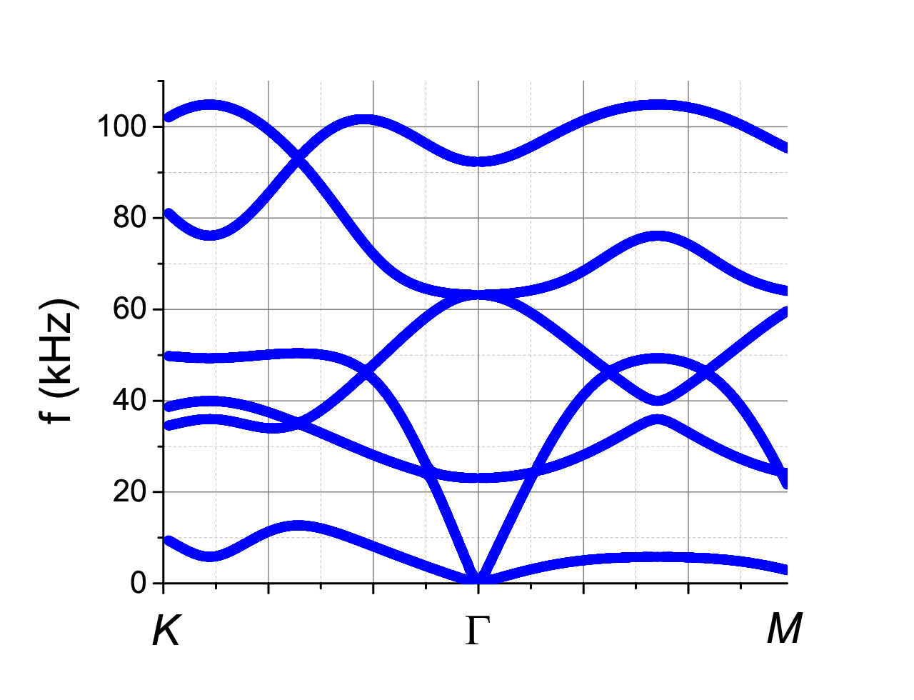
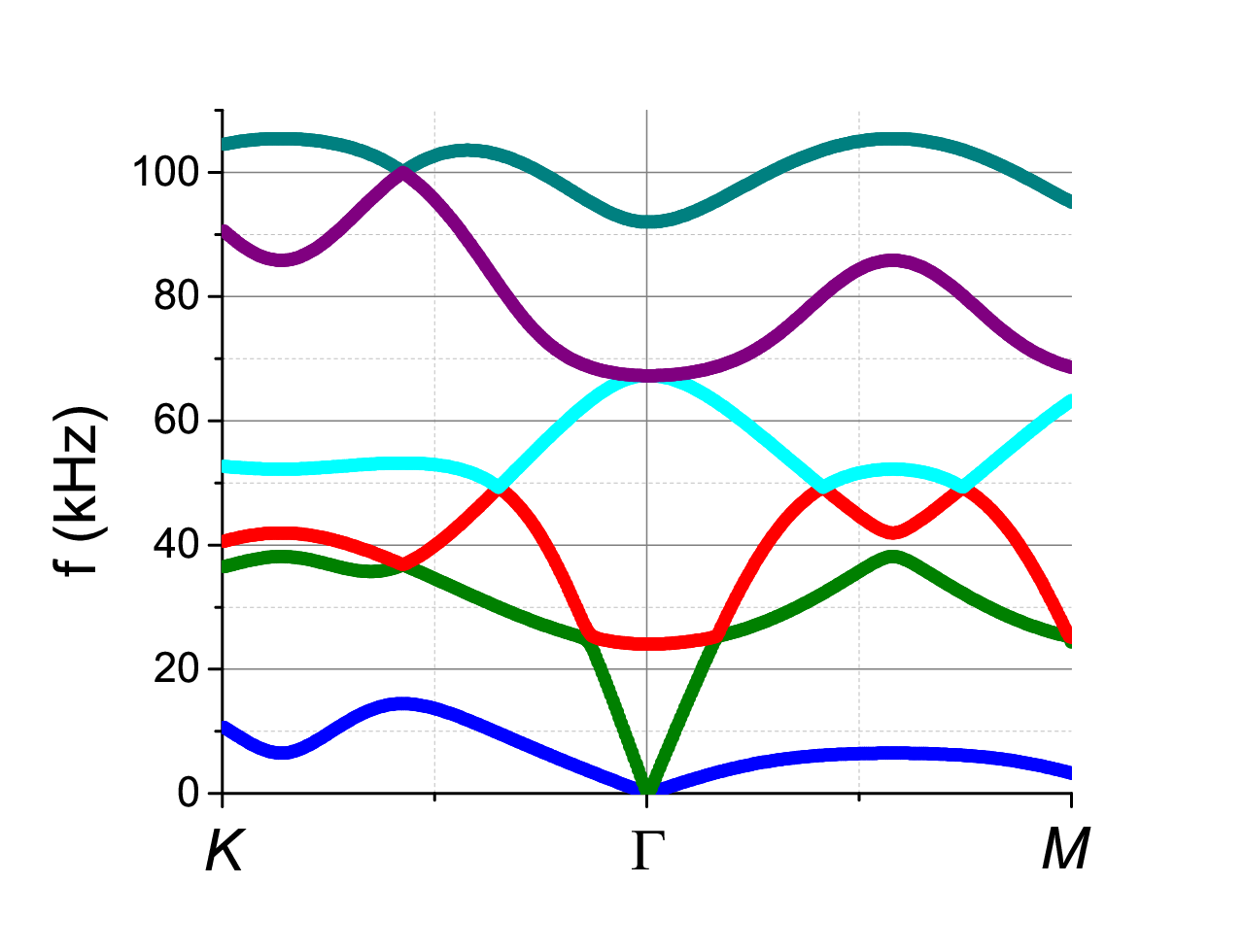
We consider an example for which all members have the same uniform properties and are arranged in a regular hexagonal lattice. The numeric computations are based on the properties in Table 2 and the path of the wave vector taken is along the perimeter of the Brillouin zone shown in Fig. 5b.

Table 2: Hexagonal lattice parameters.

$E$ (GPa)	$\nu$	$\rho^{V}$ (kg/m3)	$l$ (mm)	$t$ (mm)
70	.33	2.7 $\cdot$ 103	10	1

The dispersion curves in Fig. 6(a) were obtained from eq. (9) using a combination of minimum value threshold and minimum peak finding methods for the $6\times 6$ determinant evaluated on a discretized grid of wave vector and frequency. This provides a fast solution technique, which can be refined by taking smaller grid steps. Figure 6 shows that the dispersion curves computed by the present simplified theory agree well with those found using FEM. A close comparison shows some small deviations from the FEM results (which can safely be considered as an accurate benchmark) but the overall agreement is remarkable considering the simplicity of the present approach. The hexagonal system displays a strong one-wave effect between approximately 15 and 30 kHz. In this range the dispersion is weak, as indicated by the almost straight line branches. Furthermore, the hexagonal symmetry ensures isotropy in the long-wavelength limit, which is the original reason [15] for our interest in this particular structure.

Note that the roots obtained in Fig. 6(a) were numerically checked using a symbolic algebra -generated expression for the determinant of eq. (9). Although significant speedup in computing time was not observed, this was not the primary purpose and future work could use such very lengthy but precise expressions to better computational advantage.

(a)

(b)

Figure 6: Dispersion curves of the regular hexagonal lattice with properties in Table 2. (a) The first six Floquet branches for wave-vector along the perimeter of the Brillouin zone. (b) Dispersion curves calculated using FEM (COMSOL). Note the almost non-dispersive one-wave behaviour between 15 and 30 kHz.

6 3D Examples

6.1 Cubic lattice

₀a₁a₅a₂a₆a₄a₃

Figure 7: Cubic unit cell

6.1.1 Dispersion relations

Similar to the rectangular lattice, the equation of motion can be written as

$$\sum\limits_{j=1,2,3,4,5,6}\big({\bf P}_{0j}^{(1)}-{\bf P}_{0j}^{(2)}{\bf e}^{i{\bf k}\cdot{\bf g}_{j}}\big){\bf u}_{0}=\omega^{2}{\bf M}_{0}{\bf u}_{0},\ \ {\bf M}_{0}=\mathrm{diag}(m_{0},m_{0},m_{0},I_{0},I_{0},I_{0}).$$ (65)

We assume the members are of three types: 1, 2, 3 for the $x$, $y$, and $z$-directions, respectively, with parameters denoted by $\rho_{j}$, ${\bf K}^{(j)}$, etc. $j=1,2,3$, then eq. (65) becomes,

$$\begin{pmatrix}\zeta_{1}&0&0&0&i\lambda_{3}K^{(3)}_{14}\sin\tilde{k}_{z}&-i\lambda_{2}K^{(2)}_{14}\sin\tilde{k}_{y}\\ 0&\zeta_{2}&0&-i\lambda_{3}K^{(3)}_{14}\sin\tilde{k}_{z}&0&i\lambda_{1}K^{(1)}_{14}\sin\tilde{k}_{x}\\ 0&0&\zeta_{3}&i\lambda_{2}K^{(2)}_{14}\sin\tilde{k}_{y}&-i\lambda_{1}K^{(1)}_{14}\sin\tilde{k}_{x}&0\\ 0&i\lambda_{3}K^{(3)}_{14}\sin\tilde{k}_{z}&-i\lambda_{2}K^{(2)}_{14}\sin\tilde{k}_{y}&\zeta_{4}&0&0\\ -i\lambda_{3}K^{(3)}_{14}\sin\tilde{k}_{z}&0&i\lambda_{1}K^{(1)}_{14}\sin\tilde{k}_{x}&0&\zeta_{5}&0\\ i\lambda_{2}K^{(2)}_{14}\sin\tilde{k}_{y}&-i\lambda_{1}K^{(1)}_{14}\sin\tilde{k}_{x}&0&0&0&\zeta_{6}\end{pmatrix}2{\bf u}_{0}$$

$$\hskip 17.00024pt\hskip 17.00024pt=\omega^{2}{\bf M}_{0}{\bf u}_{0},$$ (66)

where ${\bf k}=(k_{x},k_{y},k_{z})$, $(\tilde{k}_{x},\tilde{k}_{y},\tilde{k}_{z})=(l_{1}k_{x},l_{2}k_{y},l_{3}k_{z})$ and

$$\zeta_{1}=\lambda_{2}(K^{(2)}_{11}+K^{(2)}_{13}\cos\tilde{k}_{y})+\lambda_{3}(K^{(3)}_{11}+K^{(3)}_{13}\cos\tilde{k}_{z})+\tilde{\mu}_{1}\tilde{s}_{1}(\cot\tilde{s}_{1}-\csc\tilde{s}_{1}\cos\tilde{k}_{x}),$$ (67)

$$\zeta_{2}=\lambda_{3}(K^{(3)}_{11}+K^{(3)}_{13}\cos\tilde{k}_{z})+\lambda_{1}(K^{(1)}_{11}+K^{(1)}_{13}\cos\tilde{k}_{x})+\tilde{\mu}_{2}\tilde{s}_{2}(\cot\tilde{s}_{2}-\csc\tilde{s}_{2}\cos\tilde{k}_{y}),$$

$$\zeta_{3}=\lambda_{1}(K^{(1)}_{11}+K^{(1)}_{13}\cos\tilde{k}_{x})+\lambda_{2}(K^{(2)}_{11}+K^{(2)}_{13}\cos\tilde{k}_{y})+\tilde{\mu}_{3}\tilde{s}_{3}(\cot\tilde{s}_{3}-\csc\tilde{s}_{3}\cos\tilde{k}_{z}),$$

$$\zeta_{4}=\lambda_{2}(K^{(2)}_{22}+K^{(2)}_{24}\cos\tilde{k}_{y})+\lambda_{3}(K^{(3)}_{22}+K^{(3)}_{24}\cos\tilde{k}_{z}),$$

$$\zeta_{5}=\lambda_{3}(K^{(3)}_{22}+K^{(3)}_{24}\cos\tilde{k}_{z})+\lambda_{1}(K^{(1)}_{22}+K^{(1)}_{24}\cos\tilde{k}_{x}),$$

$$\zeta_{6}=\lambda_{1}(K^{(1)}_{22}+K^{(1)}_{24}\cos\tilde{k}_{x})+\lambda_{2}(K^{(2)}_{22}+K^{(2)}_{24}\cos\tilde{k}_{y}).$$

6.1.2 Quasi-static effective elastic moduli for the cubic lattice

Considering wave propagation in the $(100)$ and $(110)$ directions of the lattice with pure cubic symmetry ($l_{1}=l_{2}=l_{3}$ etc.) and taking the low frequency limit, we obtain

$$C_{11}={EA}/{l^{2}},\ \ C_{66}={6EI}/{l^{4}},\ \ C_{12}=0,\ \ \rho_{\text{eff}}=(3\rho Al+3m_{0})/l^{3}.$$ (68)

The moduli are in agreement with known results, e.g. [2], and the effective mass density is, as expected, identical to the actual density. $C_{12}=0$ indicates that Poisson’s ratio $\nu_{12}=0$ which can be interpreted as applying a displacement in the $(100)$ direction does not cause deformation in the $(010)$ direction.

6.1.3 Example: wave propagation in the $x-$direction

We consider wave propagation along one axis of a lattice structure with uniform material and structural properties as given in Table 3 and with members of square cross-section.

Table 3: Cubic lattice parameters.

$E$ (GPa)	$\nu$	$\rho^{V}$ (kg/m3)	$l$ (mm)	$t$ (mm)
70	.33	2.7 $\cdot$ 103	10	1

Setting $\tilde{k}_{y}=\tilde{k}_{z}=0$, we find that the first pure-longitudinal solution ${\bf u}_{0}=(1,0,0,0,0,0)^{T}$ of (66), has wavenumber $\tilde{k}_{x}$ in terms of $\omega$ as

$$\cos\tilde{k}_{x}=\cos\tilde{s}+\Big(2\lambda(K_{11}+K_{13})-\frac{1}{2}m_{0}\omega^{2}\Big)\frac{\ \sin\tilde{s}}{\tilde{\mu}\tilde{s}}.$$ (69)

The flexural solution ${\bf u}_{0}=(0,1,l,0,\alpha,\beta)^{T}$ reduces the $6\times 6$ equation of motion matrix to a $4\times 4$ one.

$$\begin{pmatrix}B-m_{0}\omega^{2}&0&0&D\\ 0&B-m_{0}\omega^{2}&-D&0\\ 0&D&C-I_{0}\omega^{2}&0\\ -D&0&0&C-I_{0}\omega^{2}\end{pmatrix}\begin{pmatrix}1\\ l\\ \alpha\\ \beta\end{pmatrix}={\bf 0},$$ (70)

where

$$B=2\tilde{\mu}\tilde{s}(\cot\tilde{s}-\csc\tilde{s})+2\lambda\big(2K_{11}+K_{13}(\cos\tilde{k}_{x}+1)\big),$$ (71)

$$C=2\lambda\big(2K_{22}+K_{24}(\cos\tilde{k}_{x}+1)\big),$$

$$D=i2\lambda K_{14}\sin\tilde{k}_{x}.$$

Then calculate the determinant to obtain the flexural dispersion relation

$$\Big(\lambda\big(2K_{11}+K_{13}(\cos\tilde{k}_{x}+1)\big)+\tilde{\mu}\tilde{s}(\cot\tilde{s}-\csc\tilde{s})-\frac{1}{2}m_{0}\omega^{2}\Big)$$ (72)

$$\times\Big(\lambda\big(2K_{22}+K_{24}(\cos\tilde{k}_{x}+1)\big)-\frac{1}{2}I_{0}\omega^{2}\Big)-\big(\lambda K_{14}\sin\tilde{k}_{x}\big)^{2}=0.$$

In addition to the propagating wave branches the model also displays pure resonances. These are modes that are independent of $k_{x}$ and hence non-propagating, i.e. with zero group velocity. They correspond to the generalized displacement ${\bf u}_{0}=(0,0,0,1,0,0)^{T}$ which represents flexural resonances (deflection in $x$-direction) of the beams oriented in the $y$- and $z$-directions. The mode is a solution of eq. (66) at resonance frequencies that satisfy

$$2\lambda\big(K_{22}+K_{24}\big)-\omega^{2}I_{0}=0.$$ (73)

In the case considered with $I_{0}=0$, eq. (73) reduces to

$$\Big(\sin\frac{\gamma l}{2}\cosh\frac{\gamma l}{2}+\cos\frac{\gamma l}{2}\sinh\frac{\gamma l}{2}\Big)\,\sin\frac{\gamma l}{2}=0$$ (74)

where $\gamma$ is the flexural wavenumber of Euler beam theory. The first two lowest solutions of eq. (74) are $\gamma l=1.5000\pi$ and $2\pi$.

The dispersion curves for the cubic lattice are shown in Fig. 8. The analytic results for the propagating wave branches eqs. (69) and (72) match with the FEM simulation. The first two resonance frequencies of eq. (74) are at $51.949$ kHz and $92.354$ kHz, and are shown as flat branches in Fig. 8(a). The first/lowest solution corresponds to the flat branch in Fig. 8(b). The branch in Fig. 8(b) corresponding to the $92.354$ kHz resonance shows slight variation with wavenumber, but is well approximated by the flat branch in Fig. 8(a). We can conclude from the comparison in Fig. 8 that the analytical model predicts the first eight branches to a remarkable degree of approximation.

(a)

(b)

Figure 8: Dispersion curves of the cubic lattice of Table 3. (a) The green lines are dispersion curves of longitudinal waves, the black and red lines are dispersion curves of shear waves, and the blue curves are flexural resonances of the beams oriented in the $y$- and $z$-directions. (b) Dispersion curves calculated using FEM (COMSOL).

6.2 Tetrahedral lattice

(a)

(b)

Figure 9: Tetrahedral lattice. (a) The unit cell. (b) The irreducible Brillouin zone [16].

6.2.1 Numerical result

We consider an example for which all members are rods of radius $t$ and have the same uniform properties and are arranged in a regular tetrahedral lattice. The numerical computations are based on the properties in Table 4 and the path of the wave vector taken is along $\Gamma-{\text{L}}$ of the Brillouin zone shown in Fig. 9b.

Table 4: Tetrahedral lattice parameters.

$E$ (GPa)	$\nu$	$\rho^{V}$ (kg/m3)	$l$ (mm)	$t$ (mm)
70	.33	2.7 $\cdot$ 103	10	.5

The dispersion curves in Fig. 10(a) were obtained by finding the smallest eigenvalue of a positive definite matrix, and plotting the corresponding wave number and frequency of the discretized grid where the smallest eigenvalue is smaller than $\epsilon$ (a small value). Figure 10 shows that the dispersion curves computed by the present simplified theory agree well with those found using FEM. As with the 2D hexagonal structure, the tetrahedral lattice displays a broad frequency range with one-wave behaviour: 5 to 20 kHz. The wave is almost non-dispersive, and isotropic in the long-wavelength regime on account of the symmetry of the lattice.

(a)

(b)

Figure 10: Dispersion curves of the regular tetrahedral lattice with properties in Table 4. (a) The first seven Floquet branches for wave-vector along the perimeter of the Brillouin zone. (b) Dispersion curves calculated using FEM (COMSOL). Note the clear one-wave behaviour between about 5 and 20 kHz.

7 Conclusions

Dynamic modeling of 2D and 3D lattices can be accurately modeled using a low order model with minimal degrees of freedom described by thin beam members. The dispersion relations for rectangular and cubic lattices have been derived analytically by imposing the Bloch-Floquet periodicity condition, yielding an Hermitian eigenvalue problem for the unknown frequencies. Numerical methods were used to compute the band-diagrams for hexagonal and tetrahedral lattices. The semi-analytical approach allowed us to extract the low frequency asymptotics. In particular, the closed-form explicit expressions for the Christoffel matrix in the quasistatic regime for rectangular, hexagonal and cubic lattices were presented. Numerical comparisons of wave dispersion diagrams with FEM simulations indicate that the beam model provides good accuracy for lower modes. The semi-analytical nature of the present model makes it the natural extension of purely static methods for periodic lattice structures, e.g. [2]. It accurately predicts the one-wave behaviour in the hexagonal and tetrahedral lattices. These particular structures are distinct in that they provide effective in the long-wavelength limit, and hence quasi-acoustic wave effects in the one-wave regions. By breaking the symmetry one can extend the scalar one-wave effect to display anisotropy, an important subject for future investigation with the semi-analytic model. In summary, our beam model provides a novel and fast approach to calculate the band-diagrams for 2D and 3D lattices. This semi-analytical method may prove useful in designing phononic crystals and pentamode structures.

References

- [1] G. W. Milton and A. V. Cherkaev. Which elasticity tensors are realizable? J. Eng. Mat. Tech., 117(4):483–493, 1995.
- [2] A. N. Norris. Mechanics of elastic networks. Proc. R. Soc. A, 470:20140522+, 2014.
- [3] P. G. Martinsson and A. B. Movchan. Vibrations of lattice structures and phononic band gaps. Q. J. Mech. Appl. Math., 56(1):45–64, 2003.
- [4] A. S. Phani, J. Woodhouse, and N. A. Fleck. Wave propagation in two-dimensional periodic lattices. J. Acoust. Soc. Am., 119(4):1995–2005, 2006.
- [5] S. Gonella and M. Ruzzene. Analysis of in-plane wave propagation in hexagonal and re-entrant lattices. J. Sound. Vib., 312(1-2):125–139, 2008.
- [6] W. H. Wittrick and F. W. Williams. A general algorithm for computing natural frequencies of elastic structures. Q J Mechanics Appl Math, 24(3):263–284, 1971.
- [7] A. Spadoni, M. Ruzzene, S. Gonella, and F. Scarpa. Phononic properties of hexagonal chiral lattices. Wave Motion, 46(7):435–450, 2009.
- [8] M. J. Leamy. Exact wave-based Bloch analysis procedure for investigating wave propagation in two-dimensional periodic lattices. J. Sound. Vib., 331(7):1580–1596, 2012.
- [9] P. G. Martinsson and I. Babuška. Homogenization of materials with periodic truss or frame micro-structures. Math. Models Methods Appl. Sci., 17(5):805–832, 2007.
- [10] S. Gonella and M. Ruzzene. Homogenization and equivalent in-plane properties of two-dimensional periodic lattices. Int. J. Solids Struct., 45(10):2897–2915, 2008.
- [11] D. J. Colquitt, I. S. Jones, N. V. Movchan, and A. B. Movchan. Dispersion and localization of elastic waves in materials with microstructure. Proc. R. Soc. A, 467(2134):2874–2895, 2011.
- [12] D. J. Colquitt, M. J. Nieves, I. S. Jones, N. V. Movchan, and A. B. Movchan. Localisation for a line defect in an infinite square lattice. Proc. R. Soc. A, 469(2150):20120579, 2013.
- [13] F. W. Williams and J. R. Banerjee. Free vibration of composite beams - An exact method using symbolic computation. Journal of Aircraft, 32(3):636–642, May 1995.
- [14] Martin Maldovan and Edwin L. Thomas. Periodic Materials and Interference Lithography: For Photonics, Phononics and Mechanics. Wiley-VCH, 2009.
- [15] A.N. Norris and A.J. Nagy. Metal Water: A metamaterial for acoustic cloaking. In Proceedings of Phononics 2011, Santa Fe, NM, USA, May 29-June 2, pages 112–113, Paper Phononics–2011–0037, 2011.
- [16] W. Setyawana and S. Curtarolo. High-throughput electronic band structure calculations: Challenges and tools. Comp. Mat. Sc., 49:299–312, 2010.