Wasserstein Discriminant Analysis Thanks:  This work was supported in part by grants from the ANR OATMIL ANR-17-CE23-0012, Normandie Region, Feder, CNRS PEPS DESSTOPT, Chaire d’excellence de l’IDEX Paris Saclay.
The authors also want to thank Alexandre Saint-Dizier, Charles Bouveyron and Julie Delon for fruitful discussion and for pointing out the class weights in Fisher Discriminant.

Abstract

Wasserstein Discriminant Analysis (WDA) is a new supervised linear dimensionality reduction algorithm. Following the blueprint of classical Fisher Discriminant Analysis, WDA selects the projection matrix that maximizes the ratio of the dispersion of projected points pertaining to different classes and the dispersion of projected points belonging to a same class. To quantify dispersion, WDA uses regularized Wasserstein distances. Thanks to the underlying principles of optimal transport, WDA is able to capture both global (at distribution scale) and local (at samples’ scale) interactions between classes. In addition, we show that WDA leverages a mechanism that induces neighborhood preservation. Regularized Wasserstein distances can be computed using the Sinkhorn matrix scaling algorithm; the optimization problem of WDA can be tackled using automatic differentiation of Sinkhorn’s fixed-point iterations. Numerical experiments show promising results both in terms of prediction and visualization on toy examples and real datasets such as MNIST and on deep features obtained from a subset of the Caltech dataset.

1 Introduction

Feature learning is a crucial component in many applications of machine learning. New feature extraction methods or data representations are often responsible for breakthroughs in performance, as illustrated by the kernel trick in support vector machines (Schölkopf and Smola, 2002) and their feature learning counterpart in multiple kernel learning (Bach et al, 2004), and more recently by deep architectures (Bengio, 2009).

Among all the feature extraction approaches, one major family of dimensionality reduction methods (Van Der Maaten et al, 2009; Burges, 2010) consists in estimating a linear subspace of the data. Although very simple, linear subspaces have many advantages. They are easy to interpret, and can be inverted, at least in a lest-squares way. This latter property has been used for instance in PCA denoising (Zhang et al, 2010). Linear projection is also a key component in random projection methods (Fern and Brodley, 2003) or compressed sensing and is often used as a first pre-processing step, such as the linear part in a neural network layer. Finally, linear projections only imply matrix products and stream therefore particularly well on any type of hardware (CPU, GPU, DSP).

Linear dimensionality reduction techniques come in all flavors. Some of them, such as PCA, are inherently unsupervised; some can consider labeled data and fall in the supervised category. We consider in this paper linear and supervised techniques. Within that category, two families of methods stand out: Given a dataset of pairs of vectors and labels $\{(\mathbf{x}_{i},y_{i})\}_{i}$, with $\mathbf{x}_{i}\in\mathbb{R}^{d}$, the goal of Fisher Discriminant Analysis (FDA) and variants is to learn a linear map $\mathbf{P}:\mathbb{R}^{d}\rightarrow\mathbb{R}^{p}$, $p\ll d$, such that the embeddings of these points $\mathbf{P}\mathbf{x}_{i}$ can be easily discriminated using linear classifiers. Mahalanobis metric learning (MML) follows the same approach, except that the quality of the embedding $\mathbf{P}$ is judged by the ability of a $k$-nearest neighbor algorithm (not a linear classifier) to obtain good classification accuracy.

FDA and MML, in both Global and Local Flavors.

FDA attempts to maximize w.r.t. $\mathbf{P}$ the sum of all distances $|\!|\mathbf{P}\mathbf{x}_{i}-\mathbf{P}\mathbf{x}_{j^{\prime}}|\!|$ between pairs of samples from different classes $c,c^{\prime}$ while minimizing the sum of all distances $|\!|\mathbf{P}\mathbf{x}_{i}-\mathbf{P}\mathbf{x}_{j}|\!|$ between pairs of samples within the same class $c$ (Friedman et al, 2001, §4.3). Because of this, it is well documented that the performance of FDA degrades when class distributions are multimodal. Several variants have been proposed to tackle this problem (Friedman et al, 2001, §12.4). For instance, a localized version of FDA was proposed by Sugiyama (2007), which boils down to discarding the computation for all pairs of points that are not neighbors.

Figure 1: Weights used for inter/intra class variances for FDA, Local FDA and WDA for different regularizations $\lambda$. Only weights for two samples from class 1 are shown. The color of the link darkens as the weight grows. FDA computes a global variance with uniform weight on all pairwise distances, whereas LFDA focuses only on samples that lie close to each other. WDA relies on an optimal transport matrix $\mathbf{T}$ that matches all points in one class to all other points in another class (most links are not visible because they are colored in white as related weights are too small). WDA has both a global (due to matching constraints) and local (due to transportation cost minimization) outlook on the problem, with a tradeoff controlled by the regularization strength $\lambda$.

On the other hand, the first techniques that were proposed to learn metrics (Xing et al, 2003) used a global criterion, namely a sum on all pairs of points. Later on, variations that focused instead exclusively on local interactions, such as LMNN (Weinberger and Saul, 2009), were shown to be far more efficient in practice. Supervised dimensionality approaches stemming from FDA or MML consider thus either global or local interactions between points, namely, either all differences $|\!|\mathbf{P}\mathbf{x}_{i}-\mathbf{P}\mathbf{x}_{j}|\!|$ have an equal footing in the criterion they optimize, or, on the contrary, $|\!|\mathbf{P}\mathbf{x}_{i}-\mathbf{P}\mathbf{x}_{j}|\!|$ is only considered for points such that $\mathbf{x}_{i}$ is close to $\mathbf{x}_{j}$.

WDA: Global and Local.

We introduce in this work a novel approach that incorporates both a global and local perspective. WDA can achieve this blend through the mathematics of optimal transport ( see for instance the recent book of Peyré and Cuturi (2018) for an introduction and exposition of some of the computational we will use in this paper). Optimal transport provides a powerful toolbox to compute distances between two empirical probability distributions. Optimal transport does so by considering all probabilistic couplings between these two measures, to select one, denoted $T$, that is optimal for a given criterion. This coupling now describes interactions at both a global and local scale, as reflected by the transportation weight $T_{ij}$ that quantifies how important the distance $|\!|\mathbf{P}\mathbf{x}_{i}-\mathbf{P}\mathbf{x}_{j}|\!|$ should be to obtain a good projection matrix $\mathbf{P}$. Indeed, such weights are decided by (i) making sure that all points in one class are matched to all points in the other class (global constraint, derived through marginal constraints over the coupling); (ii) making sure that points in one class are matched only to few similar points of the other class (local constraint, thanks to the optimality of the coupling, that is a function of local costs). Our method has the added flexibility that it can interpolate, through a regularization parameter, between an exclusively global viewpoint (identical, in that case, to FDA), to a more local viewpoint with a global matching constraint (different, in that sense, to that of purely local tools such as LMNN or Local-FDA). In mathematical terms, we adopt the ratio formulation of FDA to maximize the ratio of the regularized Wasserstein distances between inter class populations and between the intra-class population with itself, when these points are considered in their projected space:

$$\max_{\mathbf{P}\in\Delta}\quad\frac{\sum_{c,c^{\prime}>c}W_{\lambda}(\mathbf{P}\mathbf{X}^{c},\mathbf{P}\mathbf{X}^{c^{\prime}})}{\sum_{c}W_{\lambda}(\mathbf{P}\mathbf{X}^{c},\mathbf{P}\mathbf{X}^{c})}$$ (1)

where $\Delta=\{\mathbf{P}=[\mathbf{p_{1}},\dots,\mathbf{p}_{p}]\quad|\quad\mathbf{p}_{i}\in\mathbb{R}^{d},\|\mathbf{p}_{i}\|_{2}=1\quad\text{ and }\mathbf{p}_{i}^{\top}\mathbf{p}_{j}=0\text{ for }i\neq j\}$ is the Stiefel manifold (Absil et al, 2009), the set of orthogonal $d\times p$ matrices; $\mathbf{P}\mathbf{X}^{c}$ is the matrix of projected samples from class $c$. $W_{\lambda}$ is the regularized Wasserstein distance proposed by Cuturi (2013), which can be expressed as $W_{\lambda}(\mathbf{X},\mathbf{Z})=\sum_{i,j}T^{\star}_{i,j}\|\mathbf{x}_{i}-\mathbf{z}_{j}\|^{2}_{2}$, $T^{\star}_{i,j}$ being the coordinates of the entropic-regularized Optimal Transport (OT) matrix $\mathbf{T}^{\star}$ (see §2). These entropic-regularized Wasserstein distances measure the dissimilarity between empirical distributions by considering pairwise distances between samples. The strength of the regularization $\lambda$ controls the local information involved in the distance computation. Further analyses and intuitions on the role on the within-class distances in the optimization problem are given in the Discussion section.

When $\lambda$ is small, we will show that WDA boils down to FDA. When $\lambda$ is large, WDA tries to split apart distributions of classes by maximizing their optimal transport distance. In that process, for a given example $\mathbf{x}_{i}$ in one class, only few components $T_{i,j}$ will be activated so that $\mathbf{x}_{i}$ will be paired with few examples. Figure 1 illustrates how pairing weights $T_{i,j}$ are defined when comparing Wasserstein discriminant analysis (WDA, with different regularization strengths) with FDA (purely global), and Local-FDA (purely local) (Sugiyama, 2007). Another strong feature brought by regularized Wasserstein distances is that relations between samples (as given by the optimal transport matrix $\mathbf{T}$) are estimated in the projected space. This is an important difference compared to all previous local approaches which estimate local relations in the original space and make the hypothesis that these relations are unchanged after projection.

Paper outline.

Section 2 provides background on regularized Wasserstein distances. The WDA criterion and its practical optimization is presented in Section 3. Section 4 by discusses properties of WDA and related works. Numerical experiments are provided in Section 5. Section 6 concludes the paper and introduces perspectives.

2 Background on Wasserstein distances

Wasserstein distances, also known as earth mover distances, define a geometry over the space of probability measures using principles from optimal transport theory (Villani, 2008). Recent computational advances (Cuturi, 2013; Benamou et al, 2015) have made them scalable to dimensions relevant to machine learning applications.

Notations and Definitions.

Let $\mu=\frac{1}{n}\sum_{i}\delta_{\mathbf{x}_{i}}$, $\nu=\frac{1}{m}\sum_{i}\delta_{\mathbf{z}_{i}}$ be two empirical measures with locations in $\mathbb{R}^{d}$ stored in matrices $\mathbf{X}=[\mathbf{x}_{1},\cdots,\mathbf{x}_{n}]$ and $\mathbf{Z}=[\mathbf{z}_{1},\cdots,\mathbf{z}_{m}]$. The pairwise squared Euclidean distance matrix between samples in $\mu$ and $\nu$ is defined as $\mathbf{M}_{\mathbf{X},\mathbf{Z}}:=[|\!|\mathbf{x}_{i}-\mathbf{z}_{j}|\!|_{2}^{2}]_{ij}\in\mathbb{R}^{n\times m}.$ Let $U_{nm}$ be the polytope of $n\times m$ nonnegative matrices such that their row and column marginals are equal to $\mathbf{1}_{n}/n$ and $\mathbf{1}_{m}/m$ respectively. Writing ${\mathbf{1}}_{n}$ for the $n$-dimensional vector of ones, we have:

$$U_{nm}:=\{\mathbf{T}\in\mathbb{R}_{+}^{n\times m}\;:\;\mathbf{T}\mathbf{1}_{m}=\mathbf{1}_{n}/n,\,\mathbf{T}^{T}\mathbf{1}_{n}=\mathbf{1}_{m}/m\}.$$

Regularized Wassersein distance.

Let $\langle\mathbf{A},\mathbf{B}\,\rangle:=\tr(\mathbf{A}^{T}\mathbf{B})$ be the Frobenius dot-product of matrices. For $\lambda\geq 0$, the regularized Wasserstein distance we adopt in this paper between $\mu$ and $\nu$ is (and with a slight abuse of notation):

$$W_{\lambda}(\mu,\nu):=W_{\lambda}(\mathbf{X},\mathbf{Z}):=\langle\mathbf{T}_{\lambda},\mathbf{M}_{\mathbf{X},\mathbf{Z}}\,\rangle,$$ (2)

where $\mathbf{T}_{\lambda}$ is the solution of an entropy-smoothed optimal transport problem,

$$\mathbf{T}_{\lambda}:=\argmin_{\mathbf{T}\in U_{nm}}\,\lambda\langle\mathbf{T},\mathbf{M}_{\mathbf{X},\mathbf{Z}}\,\rangle-\Omega(\mathbf{T}),$$ (3)

where $\Omega(\mathbf{T})$ is the entropy of $\mathbf{T}$ seen as a discrete joint probability distribution, namely $\Omega(\mathbf{T}):=-\sum_{ij}t_{ij}\log(t_{ij}).$ Note that problem (3) can be solved very efficiently using Sinkhorn’s fixed-point iterations (Cuturi, 2013). The solution of the optimization problem can be expressed as:

$${\color[rgb]{0,0,0}\mathbf{T}=\diag(\mathbf{u})\mathbf{K}\diag(\mathbf{v})=\mathbf{u}{\mathbf{1}}_{m}^{T}\circ\mathbf{K}\circ{\mathbf{1}}_{n}{\mathbf{v}}^{T},}$$ (4)

where $\circ$ stands for elementwise multiplication and $\mathbf{K}$ is the matrix whose elements are $K_{i,j}=e^{-\lambda M_{i,j}}$. The Sinkhorn iterations consist in updating left/right scaling vectors $\mathbf{u}^{k}$ and $\mathbf{v}^{k}$ of the matrix $\mathbf{K}=e^{-\lambda\mathbf{M}}$. These updates take the following form for iteration $k$:

$$\mathbf{v}^{k}=\frac{{\mathbf{1}}_{m}/m}{{\mathbf{K}}^{T}\mathbf{u}^{k-1}},\quad\mathbf{u}^{k}=\frac{{\mathbf{1}}_{n}/n}{\mathbf{K}\mathbf{v}^{k}}$$ (5)

with an initialization which will be fixed to $\mathbf{u}^{0}={\mathbf{1}}_{n}$. Because it only involves matrix products, the Sinkhorn algorithm can be streamed efficiently on parallel architectures such as GPGPUs.

3 Wasserstein Discriminant Analysis

In this section we discuss optimization problem (1) and propose an efficient approach to compute the gradient of its objective.

3.1 Optimization problem.

To simplify notations, let us define a separate empirical measure for each of the $C$ classes: samples of class $c$ are stored in matrices $\mathbf{X}^{c}$; the number of samples from class $c$ is $n_{c}$. Using the definition (2) of regularized Wasserstein distance, we can write the Wasserstein Discriminant Analysis optimization problem as

$$\max_{\mathbf{P}\in\Delta}\quad \left\{J(\mathbf{P},\mathbf{T}(\mathbf{P}))=\frac{\sum_{c,c^{\prime}>c}\langle\mathbf{P}^{T}\mathbf{P},\mathbf{C}^{c,c^{\prime}}\,\rangle}{\sum_{c}\langle\mathbf{P}^{T}\mathbf{P},\mathbf{C}^{c,c}\,\rangle}\right\}$$ (6)

$$\vskip-5.69054pt\text{s.t. }\mathbf{C}^{c,c^{\prime}} =\sum_{i,j}T^{c,c^{\prime}}_{i,j}(\mathbf{x}^{c}_{i}-\mathbf{x}^{c^{\prime}}_{j})(\mathbf{x}^{c}_{i}-\mathbf{x}^{c^{\prime}}_{j})^{T},\quad\forall c,c^{\prime}$$

$$\text{and }\mathbf{T}^{c,c^{\prime}} =\small\argmin_{\mathbf{T}\in U_{n_{c}n_{c^{\prime}}}}\,\lambda\langle\mathbf{T},\mathbf{M}_{\mathbf{P}\mathbf{X}^{c},\mathbf{P}\mathbf{X}^{c^{\prime}}}\,\rangle-\Omega(\mathbf{T}),$$

which can be reformulated as the following bilevel problem

$$\max_{\mathbf{P}\in\Delta}\quad\quad J(\mathbf{P},\mathbf{T}(\mathbf{P}))$$ (7)

$$\text{s.t. }\mathbf{T}(\mathbf{P})=\argmin_{\mathbf{T}\in U_{n_{c}n_{c^{\prime}}}}\quad E(\mathbf{T},\mathbf{P})$$ (8)

where $\mathbf{T}=\{\mathbf{T}^{c,c^{\prime}}\}_{c,c^{\prime}}$ contains all the transport matrices between classes and the inner problem function $E$ is defined as

$$E(\mathbf{T},\mathbf{P})=\sum_{c,c>=c^{\prime}}\lambda\langle\mathbf{T}^{c,c^{\prime}},\mathbf{M}_{\mathbf{P}\mathbf{X}^{c},\mathbf{P}\mathbf{X}^{c^{\prime}}}\,\rangle-\Omega(\mathbf{T}^{c,c^{\prime}}).$$ (9)

The objective function $J$ can be expressed as

$$J(\mathbf{P},\mathbf{T}(\mathbf{P}))=\frac{\langle\mathbf{P}^{T}\mathbf{P},\mathbf{C}_{b}\,\rangle}{\langle\mathbf{P}^{T}\mathbf{P},\mathbf{C}_{w}\,\rangle}$$

where $\mathbf{C}_{b}=\sum_{c,c^{\prime}>c}\mathbf{C}_{c,c^{\prime}}$ and $\mathbf{C}_{w}=\sum_{c}\mathbf{C}_{c,c}$ are the between and within cross-covariance matrices that depend on $\mathbf{T}(\mathbf{P})$. Optimization problem (7)-(8) is a bilevel optimization problem, which can be solved using gradient descent (Colson et al, 2007). Indeed, $J$ is differentiable with respect to $\mathbf{P}$. This comes from the fact that optimization problems in Equation (8) are all strictly convex, making solutions of the problems unique, hence $\mathbf{T}(\mathbf{P})$ is smooth and differentiable (Bonnans and Shapiro, 1998).

Thus, one can compute the gradient of $J$ directly w.r.t. $\mathbf{P}$ using the chain rule as follows

$$\small\nabla_{\mathbf{P}}J(\mathbf{P},\mathbf{T}(\mathbf{P}))=\frac{\partial J(\mathbf{P},\mathbf{T})}{\partial\mathbf{P}}+\sum_{c,c^{\prime}\geq c}\frac{\partial J(\mathbf{P},\mathbf{T})}{\partial\mathbf{T}^{c,c^{\prime}}}\frac{\partial\mathbf{T}^{c,c^{\prime}}}{\partial\mathbf{P}}$$ (10)

The first term in gradient (10) suppose that $\mathbf{T}$ is constant and can be computed (Eq. 94-95 (Petersen et al, 2008)) as

$$\frac{\partial J(\mathbf{P},\mathbf{T})}{\partial\mathbf{P}}=\mathbf{P}\left(\frac{2}{\sigma_{w}^{2}}\mathbf{C}_{b}-\frac{2\sigma_{b}^{2}}{\sigma_{w}^{4}}\mathbf{C}_{w}\right)$$ (11)

with $\sigma_{w}^{2}=\langle\mathbf{P}^{T}\mathbf{P},\mathbf{C}_{w}\,\rangle$ and $\sigma_{b}^{2}=\langle\mathbf{P}^{T}\mathbf{P},\mathbf{C}_{b}\,\rangle$. In order to compute the second term in (10), we will separate the cases when $c=c^{\prime}$ and $c\neq c^{\prime}$ as it corresponds to their position in the fraction of Equation (6). Their partial derivative is obtained directly from the scalar product and is a weighted vectorization of the transport cost matrix

$$\frac{\partial J(\mathbf{P},\mathbf{T})}{\partial\mathbf{T}^{c,c^{\prime}\neq c}}=\text{vec}\Big(\frac{1}{{\sigma_{w}^{2}}}\mathbf{M}_{\mathbf{P}\mathbf{X}^{c},\mathbf{P}\mathbf{X}^{c^{\prime}}}\Big)\quad\text{and}\quad\frac{\partial J(\mathbf{P},\mathbf{T})}{\partial\mathbf{T}^{c,c}}=-\text{vec}\Big({\frac{\sigma_{b}^{2}}{\sigma_{w}^{4}}}\mathbf{M}_{\mathbf{P}\mathbf{X}^{c},\mathbf{P}\mathbf{X}^{c}}\Big).$$ (12)

We will see in the remaining that the main difficulty stands in computing the Jacobian ${\partial\mathbf{T}^{c,c^{\prime}}}/{\partial\mathbf{P}}$ since the optimal transport matrix is not available as a closed form. We solve this problem using instead an automatic differentiation approach wrapped around the Sinkhorn fixed point iteration algorithm.

3.2 Automatic Differentiation.

A possible way to compute the Jacobian $\partial\mathbf{T}^{c,c^{\prime}}/\partial\mathbf{P}$ is to use the implicit function theorem as in hyperparameter estimation in ML (Bengio, 2000; Chapelle et al, 2002). We detail that approach in the appendix but it requires inverting a very large matrix, and does not scale in practice. It also assumes that the exact optimal transport $\mathbf{T}_{\lambda}$ is obtained at each iteration, which is clearly an approximation since we only have the computational budget for a finite, and usually small, number of Sinkhorn iterations.

Following the gist of Bonneel et al (2016), which do not differentiate Sinkhorn iterations but a more complex fixed point iteration designed to compute Wasserstein barycenters, we propose in this section to differentiate the transportation matrices obtained after running exactly $L$ Sinkhorn iterations, with a predefined $L$. Writing $\mathbf{T}^{k}(\mathbf{P})$, for the solution obtained after $k$ iterations as a function of $\mathbf{P}$ for a given $c,c^{\prime}$ pair,

$$\mathbf{T}^{k}(\mathbf{P})=\diag(\mathbf{u}^{k})e^{-\lambda\mathbf{M}}\diag(\mathbf{v}^{k})$$

where $\mathbf{M}$ is the distance matrix induced by $\mathbf{P}$. $\mathbf{T}^{L}(\mathbf{P})$ can then be directly differentiated:

$$\frac{\partial\mathbf{T}^{k}}{\partial\mathbf{P}} =\frac{\partial[\mathbf{u}^{k}{\mathbf{1}}_{m}^{T}]}{\partial\mathbf{P}}\circ e^{-\lambda\mathbf{M}}\circ{\mathbf{1}}_{n}{\mathbf{v}^{k}}^{T}$$ (13)

$$+ \mathbf{u}^{k}{\mathbf{1}}_{m}^{T}\circ\frac{\partial e^{-\lambda\mathbf{M}}}{\partial\mathbf{P}}\circ{\mathbf{1}}_{n}{\mathbf{v}^{k}}^{T}+\mathbf{u}^{k}{\mathbf{1}}_{m}^{T}\circ e^{-\lambda\mathbf{M}}\circ\frac{\partial{[{\mathbf{1}}_{n}\mathbf{v}^{k}}^{T}]}{\partial\mathbf{P}}$$

Note that the recursion occurs as $\mathbf{u}^{k}$ depends on $\mathbf{v}^{k}$ whose is also related to $\mathbf{u}^{k-1}$. The Jacobians that we need can then be obtained from Equation (5). For instance, the gradient of one component of $\mathbf{u}^{k}{\mathbf{1}}_{m}^{T}$ at the $j$-th line is

$$\frac{\partial\mathbf{u}^{k}_{j}}{\partial\mathbf{P}}=-\frac{1/n}{[\mathbf{K}\mathbf{v}^{k}]_{j}^{2}}\Big(\sum_{i}\frac{\partial\mathbf{K}_{j,i}}{\partial\mathbf{P}}\mathbf{v}_{i}^{k}+\sum_{i}\mathbf{K}_{j,i}\frac{\partial\mathbf{v}_{i}^{k}}{\partial\mathbf{P}}\Big),$$ (14)

while for $\mathbf{v}^{k}$, we have

$$\frac{\partial\mathbf{v}^{k}_{j}}{\partial\mathbf{P}}=-\frac{1/m}{[\mathbf{K}^{T}\mathbf{u}^{k-1}]_{j}^{2}}\Big(\sum_{i}\frac{\partial\mathbf{K}_{i,j}}{\partial\mathbf{P}}\mathbf{u}_{i}^{k-1}+\sum_{i}\mathbf{K}_{i,j}\frac{\partial\mathbf{u}_{i}^{k-1}}{\partial\mathbf{P}}\Big),$$ (15)

and finally

$$\frac{\partial\mathbf{K}_{i,j}}{\partial\mathbf{P}}=-2K_{i,j}\mathbf{P}(\mathbf{x}_{i}-\mathbf{x}_{j}^{\prime})(\mathbf{x}_{i}-\mathbf{x}_{j}^{\prime})^{T}.$$

The Jacobian $\frac{\partial\mathbf{T}^{k}}{\partial\mathbf{P}}$ can be thus obtained by keeping track of all the Jacobians at each iteration and then by successively applying those equations. This approach is far cheaper than the implicit function theorem approach. Indeed, in this case, the computation of $\frac{\partial\mathbf{T}}{\partial\mathbf{P}}$ is dominated by the complexity of computing $\frac{\partial\mathbf{K}}{\partial\mathbf{P}}$ whose costs for one iteration is $O(pn^{2}d^{2})$ for $n=m$. The complexity is then linear in $L$ and quadratic in $n$.

3.3 Algorithm

In the above subsections, we have reformulated the WDA optimization problem so as to make it tractable. We have derived closed-form expressions of some elements of the gradient as well as an automatic differentiation strategy for computing gradients of the transport plans $\mathbf{T}^{c,c^{\prime}}$ with respects to $\mathbf{P}$.

Now that all these partial derivatives are computed, we can compute the gradient $\mathbf{G}^{k}=\nabla_{\mathbf{P}}J(\mathbf{P}^{k},\mathbf{T}(\mathbf{P}^{k}))$ at iteration $k$ and apply classical manifold optimization tools such as projected gradient of Schmidt (2008) or a trust region algorithm as implemented in Manopt/Pymanopt (Boumal et al, 2014; Koep and Weichwald, 2016). The latter toolbox includes tools to optimize over the Stiefel manifold, notably automatic conversions from Euclidean to Riemannian gradients. Algorithm 1 provide the steps of a projected gradient approach for solving WDA. We noted in there that at each iteration, we need to compute all the transport plans $\mathbf{T}^{c,c^{\prime}}$, which are needed for computing $\mathbf{C}_{b}$ and $\mathbf{C}_{w}$. Automatic differentiation in the last steps of Algorithm 2 takes advantage of these transport plan computations for calculating and storing partial derivatives needed for Equation 13.

From a computational complexity point of view, for each projected gradient iteration, we have the following complexity, considering that all classes are composed of $n$ samples. For one iteration of the Sinkhorn -Knopp algorithm given in Algorithm 2, $\mathbf{u}^{k}$ and $\mathbf{v}^{k}$ are of complexity $\mathcal{O}(n^{2})$ while $\{\frac{\partial\mathbf{v}_{j}^{k}}{\partial\mathbf{P}}\}_{j}$ and $\{\frac{\partial\mathbf{u}_{j}^{k}}{\partial\mathbf{P}}\}_{n}$ are both $\mathcal{O}(n^{2}dp)$. In this algorithm, complexity is dominated by the one of $\frac{\partial\mathbf{K}_{i,j}}{\partial\mathbf{P}}$ which costs is $\mathcal{O}(n^{2}d^{2}p)$, although it is computed only once. In Algorithm 1, the costs of $\mathbf{C}_{b}$ and $\mathbf{C}_{w}$ are $\mathcal{O}(n^{2}d^{2})$ and Equation (11) and (12) yields respectively a complexity of $\mathcal{O}(pd^{2})$ and $\mathcal{O}(n^{2}d^{2}p)$. Note that the cost of computing $\frac{\partial\mathbf{T}^{k}}{\partial\mathbf{P}}$ is dominated by those of $\{\frac{\partial\mathbf{v}_{j}^{k}}{\partial\mathbf{P}}\}_{j}$ and $\{\frac{\partial\mathbf{u}_{j}^{k}}{\partial\mathbf{P}}\}_{n}$. Finally, the cost computing the sum in $\mathbf{G}^{k}=\nabla_{\mathbf{P}}J(\mathbf{P}^{k},\mathbf{T}(\mathbf{P}^{k})$ achieves a global complexity of $\mathcal{O}(C^{2}n^{2}dp)$. In conclusion, our algorithm is quadratic in both the number of samples in the classes and in the original dimension of the problem.

Algorithm 1 Projected gradient algorithm for WDA

0:  $\Pi_{\Delta}$ : projection on the Stiefel manifold

1:  Initialize $k=0$, $\mathbf{P}^{0}$

2:  repeat

3:   compute all the $\mathbf{T}^{c,c^{\prime}}$ as given in Equation (8) by means of Algorithm 2

4:   compute $\mathbf{C}_{b}$ and $\mathbf{C}_{w}$

5:   compute Equation (11) for $\mathbf{P}^{k}$

6:   compute Equation (12) for $\mathbf{P}^{k}$

7:   compute $\frac{\partial\mathbf{T}^{k}}{\partial\mathbf{P}}$ using automatic differentiation based on Equations (13), (14) and (15)

8:   compute gradient $\mathbf{G}^{k}=\nabla_{\mathbf{P}}J(\mathbf{P}^{k},\mathbf{T}(\mathbf{P}^{k})$ using all above elements

9:   compute descent direction $\mathbf{D}^{k}=\Pi_{\Delta}(\mathbf{P}^{k}-\mathbf{G})-\mathbf{P}^{k}$

10:   linesearch on the step-size $\alpha_{k}$

11:   $\mathbf{P}^{k+1}\leftarrow\Pi_{\Delta}(\mathbf{P}^{k}+\alpha_{k}\mathbf{D}^{k}$)

12:   $k\leftarrow k+1$

13:  until convergence

Algorithm 2 Sinkhorn-Knopp algorithm with automatic differentiation

0:  $\mathbf{K}=e^{-\lambda\mathbf{M}_{\mathbf{P}\mathbf{X}^{c},\mathbf{P}\mathbf{X}^{c^{\prime}}}}$, $L$ the number of iterations

1:  Initialize $k=0$, $\mathbf{u}^{0}=\mathbf{1}_{n}$, $\frac{\partial\mathbf{u}_{j}^{0}}{\partial\mathbf{P}}=\mathbf{0}$ for all $j$

2:  compute $\frac{\partial\mathbf{K}_{i,j}}{\partial\mathbf{P}}$ {store these gradients for computing $\frac{\partial\mathbf{T}^{k}}{\partial\mathbf{P}}$}

3:  for $k=1$ to $L$ do

4:   compute $\mathbf{v^{k}}$ and $\mathbf{u^{k}}$ as given in Equation (5)

5:   compute $\frac{\partial\mathbf{v}_{j}^{k}}{\partial\mathbf{P}}$ for all $j$ {store these gradients for computing $\frac{\partial\mathbf{T}^{k}}{\partial\mathbf{P}}$}

6:   compute $\frac{\partial\mathbf{u}_{j}^{k}}{\partial\mathbf{P}}$ for all $j$ {store these gradients for computing $\frac{\partial\mathbf{T}^{k}}{\partial\mathbf{P}}$}

7:  end for

7:  $\mathbf{u}^{k}$, $\mathbf{v}$ and all the gradients

4 Discussions

4.1 Wasserstein Discriminant analysis : local and global.

As we have stated, WDA allows construction of both a local and global interaction of the empirical distributions to compare. Globality naturally results from the Wasserstein distance, which is a metric on probability measures, and as such it measures discrepancy between distributions at whole level. Note however that this property would have been shared by any other metric on probability measures. Locality comes as a specific feature of regularized Wasserstein distance. Indeed as made clear by the solution in Equation (4) of the entropy-smoothed optimal transport problem, weights $T_{ij}$ tend to be larger for nearby points with an exponential decrease with respect to distance between $\mathbf{P}\mathbf{x}_{i}$ and $\mathbf{P}\mathbf{x}_{j^{\prime}}$.

4.2 Regularized Wasserstein Distance and Fisher criterion.

Fisher criterion for measuring separability stands on the ratio of inter-class and intra-class variability of samples. However, this intra-class variability can be challenging to evaluate when information regarding probability distributions come only through empirical examples. Indeed, the classical $(\lambda=\infty)$ Wasserstein distance of a discrete distribution with itself is $0$, as with any other metrics for empirical distributions. Recent result by Mueller and Jaakkola (2015) also suggests that even splitting examples from one given class and computing Wasserstein distance between resulting empirical distributions will result in arbitrary small distance with high probability. This is why entropy-regularized Wasserstein distance plays a key role in our algorithm, as to the best of our knowledge, no other metrics on empirical distributions would lead to relevant intra-class measures. Indeed, $W_{\lambda}(\mathbf{P}\mathbf{X},\mathbf{P}\mathbf{X})=\langle\mathbf{P}^{\top}\mathbf{P},\mathbf{C}\rangle$ with $\mathbf{C}=\sum_{i,j}T_{i,j}(\mathbf{x}_{i}-\mathbf{x}_{j})(\mathbf{x}_{i}-\mathbf{x}_{j})^{T}$. Hence, since $\lambda<\infty$ ensures that mass of a given sample is split among its neighbours by the transport map $\mathbf{T}$, $W_{\lambda}(\mathbf{P}\mathbf{X},\mathbf{P}\mathbf{X})$ is thus non-zero and interestingly, it depends on a weighted covariance matrix $\mathbf{C}$ which, because it depends on $\mathbf{T}$, will put more emphasis on couples of neighbour examples.

More formally, we can show that minimizing $W_{\lambda}(\mathbf{P}\mathbf{X},\mathbf{P}\mathbf{X})$ with respect to $\mathbf{P}$ induces a neighbourhood preserving map $\mathbf{P}$. This means that if an example $i$ is closer to an example $j$ than an example $k$ in the original space, this relation should be preserved in the projected space. This implies that $\|\mathbf{P}\mathbf{x}_{i}-\mathbf{P}\mathbf{x}_{j}\|_{2}$ should be smaller than $\|\mathbf{P}\mathbf{x}_{i}-\mathbf{P}\mathbf{x}_{k}\|_{2}$. Then, this neighbourhood preservation can be enforced if $K_{i,j}>K_{i,k}$, which is equivalent to $M_{i,j}<M_{i,k}$, implies $T_{i,j}>T_{i,k}$. Hence, since $W_{\lambda}(\mathbf{P}\mathbf{X},\mathbf{P}\mathbf{X})=\sum_{i,j}T_{i,j}\|\mathbf{P}\mathbf{x}_{i}-\mathbf{P}\mathbf{x}_{j}\|_{2}^{2}$, the inequality $T_{i,j}>T_{i,k}$ means that examples that are close in the input space are encouraged to be close in the projected space. We show next that there exists situation in which this condition is guaranteed.

Proposition 1

Given $\mathbf{T}$ the solution of the entropy-smoothed optimal transport problem, as defined in Eq. (3), between the empirical distribution $\mathbf{P}\mathbf{X}$ on itself, $\forall i,j,k$:

$$\exists\alpha\geq 1,K_{i,j}>\alpha K_{i,k}\quad\Rightarrow\quad T_{i,j}>T_{i,k}$$

Proof

Because, we are interested in transporting $\mathbf{P}\mathbf{X}$ on $\mathbf{P}\mathbf{X}$, the resulting matrix $\mathbf{K}$ is symmetric non-negative. Then, according to Lemma 1 (see appendix), the solution matrix $\mathbf{T}$ is also symmetric. Owing to this symmetry and the properties of the Sinkhorn-Knopp algorithm, it can be shown (Knight, 2008) that there exists a non-negative vector $\mathbf{v}$ such that $T_{i,j}=K_{i,j}v_{i}v_{j}$. In addition, because this vector is the limit of a convergent sequence obtained by the Sinkhorn-Knopp algorithm, it is bounded. Let us denoted as $A$, a constant such that $\forall i,v_{i}\geq A$. Furthermore, in Lemma 2 (see appendix), we show that $\forall i,1\geq v_{i}$. Now, it is easy to prove that

$$A>\frac{K_{i,k}}{K_{i,j}}\implies v_{j}\frac{K_{i,k}}{K_{i,j}}\implies K_{i,j}v_{j}-K_{i,k}>0$$

and because $\forall j,\,v_{j}\leq 1$ and by definition $T_{i,j}=v_{i}K_{i,j}v_{j}$, we thus have $K_{i,j}v_{j}-K_{i,k}v_{k}>0\implies T_{i,j}>T_{i,k}$. in Proposition 1 we take $\alpha=\frac{1}{A}$ since $A<1$.

Note that this proposition provides us with a guarantee on a ratio $\frac{K_{i,k}}{K_{i,j}}$ between examples that induces preservation of neighbourhood. However, the constant $A$ we exhibit here is probably loose and thus, a larger ratio may still preserve locality.

4.3 Connection to Fisher Discriminant Analysis.

We show next that WDA encompasses Fisher Discriminant analysis in the limit case where $\lambda$ approaches $0$. In this case, we can see from Eq. (3) that the matrix $\mathbf{T}$ does not depends on the data. The solution $\mathbf{T}$ for each Wasserstein distance is the matrix that maximizes entropy, namely the uniform probability distribution $\mathbf{T}=\frac{1}{nm}{\mathbf{1}}_{n,m}$. The cross-covariance matrices become thus

$$\mathbf{C}^{c,c^{\prime}}=\frac{1}{n_{c}n_{c^{\prime}}}\sum_{i,j}(\mathbf{x}^{c}_{i}-\mathbf{x}^{c^{\prime}}_{j})(\mathbf{x}^{c}_{i}-\mathbf{x}^{c^{\prime}}_{j})^{T}$$

and the matrices $\mathbf{C}_{w}$ and $\mathbf{C}_{b}$ correspond then to intra- and inter-class covariances as used in FDA. Since these matrices do not depend on $\mathbf{P}$, the optimization problem (1) boils down to the usual Rayleigh quotient which can be solved using a generalized eigendecomposition of $\mathbf{C}_{w}^{-1}\mathbf{C}_{b}$ as in FDA. Note that WDA is equivalent to FDA when the classes are balanced (in the unbalanced case one needs to weight the covariances/Wasserstein distances in (1) with the class ratios). Again, we stress out that beyond this limit case and when $\lambda>0$, the smoothed optimal transport matrix $\mathbf{T}$ promotes cross-covariance matrices that are estimated from local relations as illustrated in Figure 1.

Following this connection, we want to stress again the role played by the within-class Wasserstein distances in WDA. At first, from a theoretical point of view, optimizing the ratio instead of just maximizing the between-class distance allows us to encompass well-known method such as FDA. Secondly, as we have shown in the previous subsection, minimizing the within-class distance provides interesting features such as neighbourhood preservation under mild condition.

Another intuitive benefit of minimizing the within-class distance is the following. Suppose we have several projection maps that lead to the same optimal transport matrix $\mathbf{T}$. Since $W_{\lambda}(\mathbf{P}\mathbf{X},\mathbf{P}\mathbf{X})=\sum_{i,j}T_{i,j}\|\mathbf{P}\mathbf{x}_{i}-\mathbf{P}\mathbf{x}_{j}\|_{2}^{2}$ for any $\mathbf{P}$, minimizing $W_{\lambda}(\mathbf{P}\mathbf{X},\mathbf{P}\mathbf{X})$ with respect to $\mathbf{P}$ means preferring the projection map that yields to the smaller weighted (according to $\mathbf{T}$) pairwise distance of samples in the projected space. Since for an example $i$, $\{T_{i,j}\}_{j}$ are mainly non-zero among neighbours of $i$, minimizing the within-class distance favours projection maps that tend to tighly cluster points in the same class.

4.4 Relation to other information-theoretic discriminant analysis.

Several information-theoretic criteria have been considered for discriminant analysis and dimensionality reduction. Compared to Fisher’s criteria, these ones have the advantage of going beyond a simple sketching of the data pdf based on second-order statistics. Two recent approaches are based on the idea of maximizing distance of probability distributions of data in the projection subspaces. They just differ in the choice of the metrics of pdf (one being a $L_{2}$ distance (Emigh et al, 2015) and the second one being a Wasserstein distance (Mueller and Jaakkola, 2015)). While our approach also seeks at finding projection that maximizes pdf distance, it has also the unique feature of finding projections that preserves neighbourhood. Other recent approaches have addressed the problem of supervised dimensionality reduction algorithms still from an information theoretic learning perspective but without directly maximizing distance of pdf in the projected subpaces. We discuss two methods to which we have compared with in the experimental analysis. The approach of Suzuki and Sugiyama (2013), denoted as LSDR, seeks at finding a low-rank subspace of inputs that contains sufficient information for predicting output values. In their works, the authors define the notion of sufficiency through conditional independence of the outputs and the inputs given the projected inputs and evaluate this measure through squared-loss mutual information. One major drawback of their approach is that they need to estimate a density ratio introducing thus an extra layer of complexity and an error-prone task. Similar idea has been investigated by Tangkaratt et al (2015) as they used quadratic mutual information for evaluating statistical dependence between projected inputs and outputs (the method has been named LSQMI). While they avoid the estimation of density ratio, they still need to estimate derivatives of quadratic mutual information. Like our approach, the method of Giraldo and Principe (2013) avoids density estimation for performing supervised metric learning. Indeed, the key aspect of their work is to show that the Gram matrix of some data samples can be related to some information theoretic quantities such as conditional entropy without the need of estimating pdfs. Based on this finding, they introduced a metric learning approach, coined CEML, by minimizing conditional entropy between labels and projected samples. While their approach is appealing, we believe that a direct criterion such as Fisher’s is more relevant and robust for classification purposes, as proved in our experiments.

4.5 Wasserstein distances and machine learning.

Wasserstein distances are mainly derived from the theory of optimal transport (Villani, 2008), and provide a useful way to compare probability measures. Its practical deployment in machine learning problems has been alleviated thanks to regularized versions of the original problem (Cuturi, 2013; Benamou et al, 2015). The geometry of the space of probability measures endowed with the Wasserstein metric allows to consider various objects of interest such as means or barycenters (Cuturi and Doucet, 2014; Benamou et al, 2015), and has led to generalization of PCA in the space of probability measures (Seguy and Cuturi, 2015). It has been considered in the problem of semi-supervised learning (Solomon et al, 2014), domain adaptation (Courty et al, 2016), or definition of loss functions (Frogner et al, 2015). More recently, it has also been considered in a subspace identification problem for analyzing the differences between distributions (Mueller and Jaakkola, 2015), but contrary to our approach, they only consider projections to univariate distributions, and as such do not permit to find subspaces with dimension $>1$. More recent works have proposed to use Wasserstein for measuring similarity between documents in Huang et al (2016) and propose to learn a metric that encodes class information between samples. Note that in our work we use Wasserstein between the empirical distributions and not the training samples yielding a very different approach.

Figure 2: Illustration of subspace learning methods on a nonlinearly separable 3-class toy example of dimension $d=10$ with 2 discriminant features (shown on the upper left) and 8 Gaussian noise features. Projections onto $p=2$ of the test data are reported for several subspace estimation methods.

5 Numerical experiments

In this section we illustrate how WDA works on several learning problems. First, we evaluate our approach on a simple simulated dataset with a 2-dimensional discriminative subspace. Then, we benchmark WDA on MNIST and Caltech datasets with some pre-defined hyperparameter settings for methods having some. Unless specified and justified, for LFDA and LMNN, we have set the number of neighours to $5$. For CEML, Gaussian kernel width $\sigma$ has been fixed to $\sqrt{p}$, which is the value used by Giraldo and Principe (2013) across all their experiments. For WDA, we have chosen $\lambda=0.01$ except for the toy problem. The final experiment compares performance of WDA and competitors on some UCI dataset problems, in which relevant parameters have been validated.

Note that in the spirit of reproducible research the code will be made available to the community and the Python implementation of WDA is available as part of the POT for Python Optimal Transport Toolbox (Flamary and Courty, 2017) on Github.

5.1 Practical implementation.

In order to make the method less sensitive to the dimension and scaling of the data, we propose to use a pre-computed adaptive regularization parameter for each Wasserstein distances in (1). Denote as $\lambda_{c,c^{\prime}}$ such parameter yielding thus to a distance $W_{\lambda_{c,c^{\prime}}}$. In practice, we initialize $\mathbf{P}$ with the PCA projection, and define $\lambda_{c,c^{\prime}}$ as $\lambda_{c,c^{\prime}}=\lambda(\frac{1}{n_{c}n_{c^{\prime}}}\sum_{i,j}\|\mathbf{P}x_{i}^{c}-\mathbf{P}x_{j}^{c^{\prime}}\|^{2})^{-1}$ between class $c$ and $c^{\prime}$. These values are computed a priori and fixed in the remaining iterations. They have the advantage to promote a similar regularization strength between inter and intra-class distances.

We have compared our WDA algorithms to some classical dimensionality reduction algorithms like PCA and FDA, to some locality preserving methods such as LFDA and LMNN and to some recent mutual information-based supervised dimensionality and metric learning algorithms such as LSDR and CEML mentioned above. For the last three methods, we have used the author’s implementations. We have also considered LSQMI as a competitor but did not report its performances as they were always worse than those of LSDR.

5.2 Simulated dataset.

Figure 3: Prediction error on the simulated dataset (left) with projection dimension fixed to $p=2$ and error for varying $K$ in the KNN classifier. (right) evolution of performance with different projection dimension $p$ and best $K$ in the KNN classifier.

Figure 4: Comparison of WDA performances on the simulated dataset (left) as a function of $\lambda$. (right) as a function of $\lambda$ and with different number of fixed point iterations.

This dataset has been designed for evaluating the ability of a subspace method to uncover a discrimative linear subspace when the classes are non-linearly separable. It is a 3-class problem in dimension $d=10$ with two discriminative dimensions, the remaining $8$ containing Gaussian noise. In the $2$ discriminant features, each class is composed of two modes as illustrated in the upper left part of Figure 2.

Figure 2 also illustrates the projection of test samples in two-dimensional subspaces obtained from the different approaches. We can see that for this dataset WDA, LDSR and CEML lead to a good discriminant subspace. This illustrate the importance of estimating relations between samples in the projected space as opposed to the original space as done in LMNN and LFDA. Quantitative results are illustrated in Figure 3 (left) where we reported prediction error for a K-Nearest-Neighbors classifier (KNN) for $n=100$ training examples and $n_{t}=5000$ test examples. In this simulation, all prediction errors are averaged over 20 data generations and the neighbors parameters of LMNN and LFDA have been selected empirically to maximize performances (respectively $5$ for LMNN and $1$ for LFDA). We can see in the left part of the figure that WDA, LDSR and CEML and to a lesser extent LMNN can estimate the relevant subspace, when the optimal dimension value is given to them,that is robust to the choice of $K$. Note that slightly better performances are achieved by LSDR and CEML. In the right plot of Figure 3, we show the performances of all algorithms when varying the dimension of the projected space. We note that WDA, LMNN, LSDR and LFDA achieve their best performances for $p=2$ and that prediction errors rapidly increase as $p$ is misspecified. Instead, CEML performs very well for $p\geq 2$. Being sensitive to the correct projected space dimensionality can be considered as an asset, as typically this dimension is to be optimized (e.g by cross-validation), making it easier to spot the best dimension reduction. At the contrary, CEML is robust to projected space dimensionality mis-specification at the expense of under-estimating the best reduction of dimension.

In the left plot for Figure 4 , we illustrate the sensitivity of WDA w.r.t. the regularization parameter $\lambda$. WDA returns equivalently good performance on almost a full order of magnitude of $\lambda$. This suggests that a coarse validation can be performed in practice. The right panel of Figure 4 shows the performance of the WDA for different number of inner Sinkhorn iterations $L$. We can see that even if this parameter leads to different performances for large values of $\lambda$, it is still possible find some $\lambda$ that yield near best performance even for small value of $L$.

Figure 5: Averaged prediction error on MNIST with projection dimension (left) $p=10$. (right) $p=20$.  In these plots, LSQMID has been omitted due to poor performances.

Figure 6: Averaged prediction error on the Caltech dataset along the projection dimension. In these plots, LSQMID has been omitted due to poor performances.

Figure 7: 2D tSNE of the MNIST samples projected on $p=10$ for different approaches. (first and third lines) training set ( second and fourth lines) test set.

5.3 MNIST dataset.

Our objective with this experiment is to measure how robust our approach is with only few training samples despite high-dimensionality of the problem. To this end, we draw $n=1000$ samples for training and report the KNN prediction error as a function of $k$ for the different subspace methods when projecting onto $p=10$ and $p=20$ dimensions (resp. left and right plots of Figure 5). The reported scores are averages of 20 realizations of the same experiment. We also limit the analysis to $L=10$ as the number of Sinkhorn fixed point iterations and $\lambda=0.01$. For both $p$, WDA finds a better subspace than the original space which suggests that most of the discriminant information available in the training dataset has been correctly extracted. Conversely, the other approaches struggle to find a relevant subspace in this configuration. In addition to better prediction performance, we want to emphasize that in this configuration, WDA leads to a dramatic compression of the data from 784 to 10 or 20 features while preserving most of the discriminative information.

To gain a better understanding of the corresponding embedding, we have further projected the data from the 10-dimensional space to a 2-dimensional one using t-SNE Van der Maaten and Hinton (2008). In order to make the embeddings comparable, we have used the same initializations of t-SNE for all methods. The resulting 2D projections on the test samples are shown in Figure 7. We can clearly see the overfitting behaviour of FDA, LFDA, LMNN and LDSR that separate accurately the training samples but fail to separate the test samples. Instead, WDA is able to disentangle classes in the training set while preserving generalization abilities.

5.4 Caltech dataset.

In this experiment, we use a subset described by Donahue et al (2014) of the Caltech-256 image collection Griffin et al (2007). The dataset uses features that are the output of the DeCAF deep learning architecture Donahue et al (2014). More precisely, they are extracted as the sparse activation of the neurons from the 6th fully connected layer of a convolutional network trained on ImageNet and then fine-tuned for the considered visual recognition task. As such, they form vectors of 4096 dimensions and we are looking for subspace as small as $15$. In this setting, $500$ images are considered for training, and the remaining portion of the dataset for testing ($623$ images). There are 9 different classes in this dataset. We examine in this experiment how the proposed dimensionality reduction performs when changing the subspace dimensionality. For this problem, the regularization parameter $\lambda$ of WDA was empirically set to $10^{-2}$. The K in KNN was set to $3$ which is a common standard setting for this classifier. The reported results reported in Figure 6 are averaged over 10 realizations of the same experiment. When $p\geq 5$, WDA already finds a subspace which gathers relevant discriminative information from the original space. In this experiment, LMNN yields to a better subspace for small $p$ values while WDA is the best performing method for $p\geq 6$. Those results highlight the potential interest for using WDA as linear dimensionality reduction layers in neural-nets architecture.

5.5 Running-time

For the above experiments on MNIST and Caltech, we have also evaluated the running times of the compared algorithms. The LFDA, LMNN, LDSR and CEML codes are the Matlab code that have been released by the authors. Our WDA code is Python-based and relies on the POT toolbox ( ) . All these codes have been runned on a $16$-core Intel Xeon E5-2630 CPU, operating at 2.4 GHz with GNU/Linux and 144 Gb of RAM.

Running times needed for computing learned subspaces are reported in Table 1. We first remark that LSDR is not scalable. For instance, ot needs several tenths of hour for computing the projection from $4096$ to $14$ dimensions on Caltech. More generally, we can note that our WDA algorithm scales well and is cheaper to compute than LMNN and is far less expensive than CEML on our machine. We believe our WDA algorithm better leverages multi-core machines owing the large amount of matrix-vector multiplications needed for computing Sinkorhn iterations.

Datasets	PCA	FDA	LFDA	LMNN	LSDR	CEML	WDA
Mnist (10)	0.39(0.1)	0.69(0.2)	0.55(0.4)	20.55(14.2)	29813(5048)	87.02(8.7)	6.28(0.3)
Mnist (20)	0.38(0.0)	0.58(0.0)	0.54(0.2)	18.27(17.0)	60147(11176)	90.22(8.8)	6.15(0.1)
Caltech (14)	0.53(0.3)	21.38(6.1)	11.43(2.0)	39.56(6.3)	140776(53036)	14.59(7.6)	5.29(0.1)

Table 1: Averaged running time in seconds of the different algorithms for computing the learned subspaces.

5.6 UCI datasets.

Datasets	Orig.	PCA	FDA	LFDA	LMNN	LSDR	LSQMI	CEML	WDA
wines	24.33	26.57	37.87	29.21	32.81	32.81	46.29	15.34	16.91
iris	42.07	40.60	19.27	25.13	21.67	37.93	56.27	20.87	20.87
glass	54.01	58.16	57.45	59.53	54.25	50.85	65.42	34.86	45.99
vehicles	58.68	57.26	48.57	48.25	40.84	51.86	65.09	48.46	51.13
credit	28.90	25.57	18.67	17.69	23.73	24.71	39.01	17.65	17.39
ionosphere	26.14	26.90	29.63	27.64	30.80	31.08	36.42	22.87	20.40
isolet	17.50	17.60	15.12	13.96	11.13	13.33	21.76	30.19	14.41
usps	7.59	7.66	11.63	12.76	6.05	8.77	14.83	10.15	6.50
mnist	17.26	14.16	33.85	29.92	13.95	26.53	60.05	24.68	13.07
caltechpca	23.39	13.93	12.03	18.19	11.55	36.08	100.00	13.65	11.45
Aver. Rank	5.4	5.5	5.2	5.2	3.4	5.7	8.9	3.5	2.2

Table 2: Average test errors over $20$ trials on UCI datasets. In bold, the lower test error accross algorithms. Underlined averaged test errors that are statistically non-significantly different according to a signrank test with p-val = 0.05. Result of LSQMI on caltech has not been reported due to lack of convergence after few days of computation.

We have also compared the performances of the dimensionality reduction algorithms on some UCI benchmark datasets Lichman (2013). The experimental setting is similar to the one proposed by the authors of LSQMI Tangkaratt et al (2015). For these UCI datasets, we have appended the original input features with some noise features of dimensionality $100$. We have split the examples $50\%-50\%$ in a training and test set. Hyper-parameters such as the number of neighbours for the KNN and and the dimensionality of the projection has been cross-validated on the training set and choosed respectively among the values $[1:2:19]$ (in Matlab notation) and $[5,10,15,20,25]$. Splits have been performed $20$ times. Note that we have also added experiments with Isolet, USPS, MNIST and Caltech datasets under this validation setting but without the additional noisy features. Table 2 presents the performance of competing methods. We note that our WDA is more robust than all other methods and is able to capture relevant information in the learned subspaces. Its average ranking on all datasets is $2.2$ while the second best, LMNN is $3.4$. There is only one dataset (vehicles) for which WDA performs significantly worse than top methods. Interestingly LSDR and LSQMI seem to be less robust than LMNN and FDA, against which they have not been compared in the original paper (Tangkaratt et al, 2015).

6 Conclusion

This work presents the Wasserstein Discriminant Analysis, a new and original linear discriminant subspace estimation method. Based on the framework of regularized Wasserstein distances, which measure a global similarity between empirical distributions, WDA operates by separating distributions of different classes in the subspace, while maintaining a coherent structure at a class level. To this extent, the use of regularization in the Wasserstein formulation allows to effectively bridge a gap between a global coherency and the local structure of the class manifold. This comes at a cost of a difficult optimization of a bi-level program, for which we proposed an efficient method based on automatic differentiation of the Sinkhorn algorithm. Numerical experiments show that the method performs well on a variety of features, including those obtained with a deep neural architecture. Future work will consider stochastic versions of the same approach in order to enhance further the ability of the method to handle large volume of high-dimensional data.

Appendix A Illustration of the transport $\mathbf{T}^{c,c^{\prime}}$

In this Section, we provide intuition on how the transport $\mathbf{T}^{c,c^{\prime}}$ between class $c$ and $c^{\prime}$ behaves in 2D toy problem. Remind that this matrix plays an essential role on how the covariance matrix $\mathbf{C}$ is estimated in Equation (6).

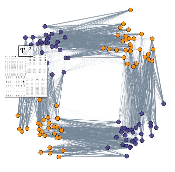
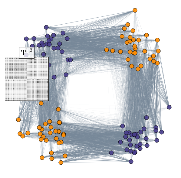
In this example, illustrated in Figure 8, two bi-modal Gaussian distributions are sampled to produce two distributions representing two classes. We illustrate in Figure 9 the transport $\mathbf{T}^{1,2}$ (inter-class) and $\{\mathbf{T}^{1,1}\mathbf{T}^{2,2}\}$ (intra-class). The corresponding transport matrices are either displayed in matrix form as inserts, or as connections between the samples. Those connections have a width parametrized by the magnitude of the connection (i.e. a small $t_{i,j}$ value will be displayed as a very thin connection). We note that for visualization purpose, the magnitude of the $\mathbf{T}$ elements displayed in matrix form are normalized by the the largest magnitude in the matrix. The transport maps can be observed in Figure 9 for three different values of the $\lambda$ parameter ($\lambda=1,0.5,0.1$). One can notice the locality induced by large values of $\lambda$, which allows to concentrate the connections on specific modes of the distributions. When $\lambda$ is smaller, inter-modes connections start to appear, which allows to consider the data distributions at a larger scale when computing $\mathbf{C}$. Regarding the inter-class transport $\mathbf{T}^{1,2}$ , one can also observe the specific relations induced by the optimal transport maps, that do not associate modes together, but rather dispatch one mode of each class onto the two modes of the other.

Figure 8: Illustration of the evolution of the transport for two classes $c=1$ and $c^{\prime}=2$

Figure 9: Illustration of the evolution of the transport for two classes for three values of the $\lambda$ parameter (first row) $\lambda=1$ (second row) $\lambda=0.5$ (last row) $\lambda=0.1$. The left column illustrates inter-class relations, while the right column illustrates intra-class relations.

Appendix B Implicit function gradient computation

In this section, we propose to compute this Jacobian based on the implicit function theorem.

For clarity’s sake, in this subsection we will not use the $c,c^{\prime}$ indices and $\mathbf{T}$ represents an optimal transport matrix between $n$ and $m$ samples projected with $\mathbf{P}$. First, we express the function $\mathbf{T}(\mathbf{P})$ as an implicit function using the optimality conditions of the equation defining the optimal $\mathbf{T}$ in Equation 6. The Lagrangian of this problem can be expressed as Cuturi (2013):

$$\small\mathcal{L}= \sum_{i,j}\left(t_{i,j}m_{i,j}(\mathbf{P})+t_{i,j}\log(t_{i,j})\right)$$

$$+\sum_{i}\alpha_{i}\left(\sum_{j}t_{i,j}-r_{i}\right)+\sum_{j}\beta_{j}\left(\sum_{i}t_{i,j}-c_{j}\right)$$

where $\boldsymbol{\alpha}$ and $\boldsymbol{\beta}$ are the dual variables associated to the sum constraints, $m_{i,j}=\|\mathbf{P}\mathbf{x}_{i}-\mathbf{P}\mathbf{z}_{j}\|^{2}$ and in our particular case $r_{i}=\frac{1}{n}$ and $c_{j}=\frac{1}{m},\forall i,j$. One can define an implicit fonction $g(\mathbf{P},\mathbf{T},\boldsymbol{\alpha},\boldsymbol{\beta}):\mathbb{R}^{p\times d+n\times m+n+m}\rightarrow\mathbb{R}^{n\times m+n+m}$ from the above lagrangian by computing its gradient w.r.t. ($\mathbf{T},\boldsymbol{\alpha},\boldsymbol{\beta}$) and setting it to zero owing to optimality. The implicit function theorem gives us the following relation:

$$\nabla_{\mathbf{P}}g=\frac{\partial g}{\partial\mathbf{P}}+\frac{\partial g}{\partial\mathbf{T}}\frac{\partial\mathbf{T}}{\partial\mathbf{P}}+\frac{\partial g}{\partial\boldsymbol{\alpha}}\frac{\partial\boldsymbol{\alpha}}{\partial\mathbf{P}}+\frac{\partial g}{\partial\boldsymbol{\beta}}\frac{\partial\boldsymbol{\beta}}{\partial\mathbf{P}}=\mathbf{0}$$

which can be reformulated as

$$\begin{bmatrix}\displaystyle\frac{\partial\mathbf{T}}{\partial\mathbf{P}}\\ \displaystyle\frac{\partial\boldsymbol{\alpha}}{\partial\mathbf{P}}\\ \displaystyle\frac{\partial\boldsymbol{\beta}}{\partial\mathbf{P}}\end{bmatrix}=-\mathbf{E}^{-1}\frac{\partial g}{\partial\mathbf{P}},\quad\text{ with }\quad\mathbf{E}=\begin{bmatrix}\displaystyle\frac{\partial g}{\partial\mathbf{T}}&\displaystyle\frac{\partial g}{\partial\boldsymbol{\alpha}}&\displaystyle\frac{\partial g}{\partial\boldsymbol{\beta}}\end{bmatrix}$$ (16)

when the function is well defined and $\mathbf{E}$ is invertible. The derivative $\frac{\partial\mathbf{T}}{\partial\mathbf{P}}$ can be deduced from the upper part of the term on the left. Note that all the partial derivatives in Equ. (16) are easy to compute. Additionally, $\mathbf{E}$ is a $(pd+nm+n+m)\times(pd+nm+n+m)$ matrix which is very sparse, as shown in the sequel. However, assuming for instance that the number of points in each class $m=n$ is the same, using this technique would amount to solve a large $n^{2}\times n^{2}$ linear system with a worst case complexity of $O(n^{6})$.

We now detail the computation of the gradient using the implicit function theorem. Note that we use the notation of the paper and that we want to compute the Jacobian $\frac{\partial\mathbf{T}}{\partial\mathbf{P}}$. First we compute the implicit function $g(\mathbf{P},\mathbf{T},\boldsymbol{\alpha},\boldsymbol{\beta}):\mathbb{R}^{p\times d+n\times m+n+m}\rightarrow\mathbb{R}^{n\times m+n+m}$ from the Lagrangian function given in the paper by computing the OT problem optimality conditions:

$$\frac{\partial\mathcal{L}}{\partial t_{k,l}} =\lambda(\mathbf{x}_{k}-\mathbf{z}_{l})^{\top}\mathbf{P}^{\top}\mathbf{P}(\mathbf{x}_{k}-\mathbf{z}_{l})+\log(t_{k,l})$$

$$\quad+1+\alpha_{k}+\beta_{l}=0$$

$$\frac{\partial\mathcal{L}}{\partial\alpha_{i}} =\sum_{j}t_{i,j}-r_{i}=0$$

$$\frac{\partial\mathcal{L}}{\partial\beta_{j}} =\sum_{i}t_{i,j}-c_{j}=0$$

$\forall k,l,i,j$. The Jacobian $\frac{\partial\mathbf{T}}{\partial\mathbf{P}}$ can be computed using the implicit function by solving the following linear problem:

$$\begin{bmatrix}\displaystyle\frac{\partial\mathbf{T}}{\partial\mathbf{P}}\\ \displaystyle\frac{\partial\boldsymbol{\alpha}}{\partial\mathbf{P}}\\ \displaystyle\frac{\partial\boldsymbol{\beta}}{\partial\mathbf{P}}\end{bmatrix}=-\mathbf{E}^{-1}\frac{\partial g}{\partial\mathbf{P}},\quad\text{ with }\quad\mathbf{E}=\begin{bmatrix}\displaystyle\frac{\partial g}{\partial\mathbf{T}}&\displaystyle\frac{\partial g}{\partial\boldsymbol{\alpha}}&\displaystyle\frac{\partial g}{\partial\boldsymbol{\beta}}\end{bmatrix}$$ (17)

First $\mathbf{t}=\text{vec}(\mathbf{T})$ is vectorized as in Matlab with column major format.

$$\frac{\partial g}{\partial\mathbf{T}}=\begin{bmatrix}\text{diag}(\frac{1}{\mathbf{t}})\\ \mathbf{I}_{n}\mathbf{I}_{n},\dots,\mathbf{I}_{n}\\ \mathbf{L}_{m,n}^{1}\mathbf{L}_{m,n}^{2},\dots,\mathbf{L}_{m,n}^{m}\end{bmatrix}$$ (18)

where $\mathbf{L}_{m,n}^{k}$ is $\mathbb{R}^{m\times n}$ matrix of $0$ with all coefficients on line $k$ equal to 1.

$$\frac{\partial g}{\partial\boldsymbol{\alpha}}=\begin{bmatrix}{\mathbf{I}_{n}}\\ {\mathbf{I}_{n}}\\ \ldots\\ {\mathbf{I}_{n}}\\ \mathbf{0}_{n,n}\\ \mathbf{0}_{m,n}\end{bmatrix}\quad\quad\quad\frac{\partial g}{\partial\boldsymbol{\beta}}=\begin{bmatrix}{\mathbf{L}_{m,n}^{1}}^{\top}\\ {\mathbf{L}_{m,n}^{2}}^{\top}\\ \ldots\\ {\mathbf{L}_{m,n}^{m}}^{\top}\\ \mathbf{0}_{n,n}\\ \mathbf{0}_{m,n}\end{bmatrix}$$ (19)

Now we compute the last element $\frac{\partial g}{\partial\mathbf{P}}$ using a vectorization $\mathbf{p}=\text{vec}(\mathbf{P})$ and $\Delta_{i,j}=\mathbf{x}_{i}-\mathbf{z}_{j}$ First note that

$$\frac{\partial\mathbf{x}^{\top}\mathbf{P}^{\top}\mathbf{P}\mathbf{x}}{\partial p_{m,l}}=2x_{l}\sum_{i}x_{i}p_{m,i}=2x_{l}(\mathbf{P}(m,:)\mathbf{x})$$

which leads to the following Jacobian

$$\frac{\partial g}{\partial\mathbf{P}}=2\lambda\begin{bmatrix}\Delta_{1,1}^{\top}\otimes\Delta_{1,1}^{\top}\mathbf{P}^{\top}\\ \Delta_{2,1}^{\top}\otimes\Delta_{2,1}^{\top}\mathbf{P}^{\top}\\ \ldots\\ \Delta_{n,m}^{\top}\otimes\Delta_{n,m}^{\top}\mathbf{P}^{\top}\\ \mathbf{0}_{n+m,dp}\end{bmatrix}$$ (20)

where the upper part of the matrix can be seen as a column-only Kroenecker product between $\Delta$ and $\mathbf{P}\Delta$.

All the elements are now in place for the linear system (17), which can be solved using any efficient method for sparse linear system.

Appendix C Lemmas

Lemma 1

If the matrix $\mathbf{M}\in\mathbb{R}^{n\times n}$ is non-negative symmetric then the matrix $\mathbf{T}$ defined as in

$$\argmin_{\mathbf{T}\in U_{n,n}}\lambda\langle\mathbf{T},\mathbf{M}\rangle-\Omega(\mathbf{T})$$

is also symmetric non-negative. Here, $\Omega$ is the entropy of the matrix $\mathbf{T}$

Proof

As this optimization problem is strictly convex for $\lambda<\infty$, and thus admits an unique solution. We show in the sequel that $\mathbf{T}^{\top}$ achieves the same objective value than $\mathbf{T}$ and thus $\mathbf{T}^{\top}$ is also a minimizer, which naturally leads to $\mathbf{T}^{\top}=\mathbf{T}$.

First note that the constraints are symmetric thus, $\mathbf{T}^{\top}$ is feasible. In addition because the entropy only depends on single entries of the matrix hence $\Omega(\mathbf{T})=\Omega(\mathbf{T}^{\top})$. Finally,

$$\langle\mathbf{T}^{\top},\mathbf{M}\rangle =\sum_{i,j}M_{i,j}T^{\top}_{i,j}=\sum_{i,j}M_{i,j}T_{j,i}=\sum_{i,j}M_{j,i}T_{j,i}$$

$$=\langle\mathbf{T},\mathbf{M}\rangle$$

which proves that both matrices lead to the same objective values.

Lemma 2

Suppose that $\mathbf{T}$ is the solution of an entropy-smoothed optimal transport problem, with matrix $\mathbf{K}$ being symmetric and such that $\forall i,K_{i,i}=1$. There exists a vector $\mathbf{v}$ such that $\forall i,j,\mathbf{T}_{i,j}=\mathbf{K}_{i,j}\mathbf{v}_{i}\mathbf{v}_{j}$ and $\forall i,\mathbf{v}_{i}\leq 1$.

Proof

Existence of the $\mathbf{v}$ such that $\mathbf{T}_{i,j}=\mathbf{K}_{i,j}\mathbf{v}_{i}\mathbf{v}_{j}$ comes from the fact that the optimization problem can be solved using the Sinkhorn-Knopp algorithm. Through the constraints of the optimal transport problem, we have

$$\forall i,j\,\,\mathbf{T}_{i,j}=\mathbf{K}_{i,j}\mathbf{v}_{i}\mathbf{v}_{j}\leq\frac{1}{n}.$$

When, $i=j$, as $\mathbf{K}_{i,i}=1$, we have $\mathbf{v}_{i}^{2}\leq\frac{1}{n}$ and thus $\mathbf{v}_{i}\leq 1$.

References

- Absil et al (2009) Absil PA, Mahony R, Sepulchre R (2009) Optimization algorithms on matrix manifolds. Princeton University Press
- Bach et al (2004) Bach FR, Lanckriet GR, Jordan MI (2004) Multiple kernel learning, conic duality, and the smo algorithm. In: Proceedings of the twenty-first international conference on Machine learning, ACM, p 6
- Benamou et al (2015) Benamou JD, Carlier G, Cuturi M, Nenna L, Peyré G (2015) Iterative bregman projections for regularized transportation problems. SIAM Journal on Scientific Computing 37(2):A1111–A1138
- Bengio (2000) Bengio Y (2000) Gradient-based optimization of hyperparameters. Neural computation 12(8):1889–1900
- Bengio (2009) Bengio Y (2009) Learning deep architectures for ai. Foundations and trends® in Machine Learning 2(1):1–127
- Bonnans and Shapiro (1998) Bonnans JF, Shapiro A (1998) Optimization problems with perturbations: A guided tour. SIAM review 40(2):228–264
- Bonneel et al (2016) Bonneel N, Peyré G, Cuturi M (2016) Wasserstein barycentric coordinates: Histogram regression using optimal transport. ACM Transactions on Graphics 35(4)
- Boumal et al (2014) Boumal N, Mishra B, Absil PA, Sepulchre R (2014) Manopt, a matlab toolbox for optimization on manifolds. The Journal of Machine Learning Research 15(1):1455–1459
- Burges (2010) Burges CJ (2010) Dimension reduction: A guided tour. Now Publishers
- Chapelle et al (2002) Chapelle O, Vapnik V, Bousquet O, Mukherjee S (2002) Choosing multiple parameters for support vector machines. Machine learning 46(1-3):131–159
- Colson et al (2007) Colson B, Marcotte P, Savard G (2007) An overview of bilevel optimization. Annals of operations research 153(1):235–256
- Courty et al (2016) Courty N, Flamary R, Tuia D, Rakotomamonjy A (2016) Optimal transport for domain adaptation. Pattern Analysis and Machine Intelligence, IEEE Transactions on
- Cuturi (2013) Cuturi M (2013) Sinkhorn distances: Lightspeed computation of optimal transport. In: NIPS, pp 2292–2300
- Cuturi and Doucet (2014) Cuturi M, Doucet A (2014) Fast computation of wasserstein barycenters. In: ICML
- Donahue et al (2014) Donahue J, Jia Y, Vinyals O, Hoffman J, Zhang N, Tzeng E, Darrell T (2014) DeCAF: a deep convolutional activation feature for generic visual recognition. In: Proceedings of The 31st International Conference on Machine Learning, pp 647–655
- Emigh et al (2015) Emigh M, Kriminger E, Prîncipe JC (2015) Linear discriminant analysis with an information divergence criterion. In: 2015 International Joint Conference on Neural Networks (IJCNN), IEEE, pp 1–6
- Fern and Brodley (2003) Fern XZ, Brodley CE (2003) Random projection for high dimensional data clustering: A cluster ensemble approach. In: ICML, vol 3, pp 186–193
- Flamary and Courty (2017) Flamary R, Courty N (2017) Pot python optimal transport library
- Friedman et al (2001) Friedman J, Hastie T, Tibshirani R (2001) The elements of statistical learning. Springer series in statistics Springer, Berlin
- Frogner et al (2015) Frogner C, Zhang C, Mobahi H, Araya M, Poggio T (2015) Learning with a wasserstein loss. In: NIPS, pp 2044–2052
- Giraldo and Principe (2013) Giraldo LGS, Principe JC (2013) Information theoretic learning with infinitely divisible kernels. In: Proceedings of the first International Conference on Representation Learning (ICLR), pp 1–8
- Griffin et al (2007) Griffin G, Holub A, Perona P (2007) Caltech-256 Object Category Dataset. Tech. Rep. CNS-TR-2007-001, California Institute of Technology
- Huang et al (2016) Huang G, Guo C, Kusner MJ, Sun Y, Sha F, Weinberger KQ (2016) Supervised word mover’s distance. In: Advances in Neural Information Processing Systems, pp 4862–4870
- Knight (2008) Knight PA (2008) The sinkhorn–knopp algorithm: convergence and applications. SIAM Journal on Matrix Analysis and Applications 30(1):261–275
- Koep and Weichwald (2016) Koep N, Weichwald S (2016) Pymanopt: A python toolbox for optimization on manifolds using automatic differentiation. Journal of Machine Learning Research 17:1–5
- Lichman (2013) Lichman M (2013) UCI machine learning repository. URL http://archive.ics.uci.edu/ml
- Van der Maaten and Hinton (2008) Van der Maaten L, Hinton G (2008) Visualizing data using t-sne. Journal of Machine Learning Research 9(2579-2605):85
- Mueller and Jaakkola (2015) Mueller J, Jaakkola T (2015) Principal differences analysis: Interpretable characterization of differences between distributions. In: NIPS, pp 1693–1701
- Petersen et al (2008) Petersen KB, Pedersen MS, et al (2008) The matrix cookbook. Technical University of Denmark 7:15
- Peyré and Cuturi (2018) Peyré G, Cuturi M (2018) Computational Optimal Transport. To be published in Foundations and Trends in Computer Science, URL https://optimaltransport.github.io
- Schmidt (2008) Schmidt M (2008) Minconf-projection methods for optimization with simple constraints in matlab
- Schölkopf and Smola (2002) Schölkopf B, Smola AJ (2002) Learning with kernels: Support vector machines, regularization, optimization, and beyond. MIT press
- Seguy and Cuturi (2015) Seguy V, Cuturi M (2015) Principal geodesic analysis for probability measures under the optimal transport metric. In: NIPS, pp 3294–3302
- Solomon et al (2014) Solomon J, Rustamov R, Leonidas G, Butscher A (2014) Wasserstein propagation for semi-supervised learning. In: ICML, pp 306–314
- Sugiyama (2007) Sugiyama M (2007) Dimensionality reduction of multimodal labeled data by local fisher discriminant analysis. The Journal of Machine Learning Research 8:1027–1061
- Suzuki and Sugiyama (2013) Suzuki T, Sugiyama M (2013) Sufficient dimension reduction via squared-loss mutual information estimation. Neural computation 25(3):725–758
- Tangkaratt et al (2015) Tangkaratt V, Sasaki H, Sugiyama M (2015) Direct estimation of the derivative of quadratic mutual information with application in supervised dimension reduction. arXiv preprint arXiv:150801019
- Van Der Maaten et al (2009) Van Der Maaten L, Postma E, Van den Herik J (2009) Dimensionality reduction: a comparative review. Journal of Machine Learning Research 10:66–71
- Villani (2008) Villani C (2008) Optimal transport: old and new, vol 338. Springer Science & Business Media
- Weinberger and Saul (2009) Weinberger KQ, Saul LK (2009) Distance metric learning for large margin nearest neighbor classification. The Journal of Machine Learning Research 10:207–244
- Xing et al (2003) Xing EP, Ng AY, Jordan MI, Russell S (2003) Distance metric learning with application to clustering with side-information. Advances in neural information processing systems 15:505–512
- Zhang et al (2010) Zhang L, Dong W, Zhang D, Shi G (2010) Two-stage image denoising by principal component analysis with local pixel grouping. Pattern Recognition 43(4):1531–1549
Appendix A Illustration of the transport