On Takens’ Last Problem:
tangencies and time averages near heteroclinic networks Thanks: CMUP (UID/MAT/00144/2013) is supported by the European Regional Development Fund through the programme COMPETE and by the Portuguese Government through the Fundação para a Ciência e a Tecnologia (FCT) under the partnership agreement PT2020. A.A.P. Rodrigues was supported by the grant SFRH/BPD/84709/2012 of FCT. Part of this work has been written during AR stay in Nizhny Novgorod University partially supported by the grant RNF 14-41-00044.

Abstract

We obtain a robust family of smooth ordinary differential equations exhibiting heteroclinic tangencies for a dense subset of parameters. We use this to find dense subsets of parameter values such that the set of solutions with historic behaviour contains an open set. This provides an affirmative answer to Taken’s Last Problem (F. Takens (2008) Nonlinearity, 21(3) T33–T36). A limited solution with historic behaviour is one for which the time averages do not converge as time goes to infinity. Takens’ problem asks for dynamical systems where historic behaviour occurs persistently for initial conditions in a set with positive Lebesgue measure.

The family appears in the unfolding of a degenerate differential equation whose flow has an asymptotically stable heteroclinic cycle involving two-dimensional connections of non-trivial periodic solutions. We show that the degenerate problem also has historic behaviour, since for an open set of initial conditions starting near the cycle, the time averages approach the boundary of a polygon whose vertices depend on the centres of gravity of the periodic solutions and their Floquet multipliers.

We illustrate our results with an explicit example where historic behaviour arises in the unfolding of an SO(2)-equivariant vector field.

Keywords: Heteroclinic cycle, Time averages, Historic behaviour, Heteroclinic tangencies, Newhouse phenomena.

2010 — AMS Subject Classifications

Primary: 34C28; Secondary: 34C37, 37C29, 37D05, 37G35

1 Introduction

Chaotic dynamics makes it difficult to give a geometric description of an attractor in many situations, when probabilistic and ergodic analysis becomes relevant. In a long record of a chaotic signal generated by a deterministic time evolution, for suitable initial conditions the expected time average exists — see [29, 30]. However, there are cases where the time averages do not converge no matter how long we wait. This historic behaviour is associated with intermittent dynamics, which happens typically near heteroclinic networks.

The aim of this article is to explore the persistence of this behaviour for a deterministic class of systems involving robust heteroclinic cycles, leading to an answer to Taken’s Last Problem [34]. More precisely, we study non-hyperbolic heteroclinic attractors such that the time averages of all solutions within their basin of attraction do not converge, and for which this holds persistently.

This is done by first studying a one-parameter family of vector fields having periodic solutions connected in a robust cycle. We show that under generic conditions there are parameter values for which the invariant manifolds of a pair of periodic solutions have a heteroclinic tangency. This implies the Newhouse property of existence of infinitely many sinks. Results by Kiriki and Soma [18] may then be used to provide an affirmative answer to the problem proposed by Takens in [34].

1.1 Takens’ last problem

Let $M$ be a compact three-dimensional manifold without boundary and consider a vector field $f:M\rightarrow TM$ defining a differential equation

$$\dot{x}=f(x),\qquad x(0)=x_{0}\in M$$ (1.1)

and denote by $\phi(t,x_{0})$, with $t\in{\rm\bf R}$, the associated flow with initial condition $x_{0}\in M$. The following terminology has been introduced by Ruelle [29] (see also Sigmund [30]).

Definition 1

We say that the solution $\phi(t,x_{0})$, $x_{0}\in M$, of (1.1) has historic behaviour if there is a continuous function $g:M\rightarrow{\rm\bf R}$ such that the time average

$$\frac{1}{T}\int_{0}^{T}g(\phi(t,x_{0}))dt$$ (1.2)

fails to converge.

A solution $\phi(t,x_{0})$, $x_{0}\in M$ with historic behaviour retains informations about its past. This happens, in particular, if there are at least two different sequences of times, say $(T_{i})_{i\in{\rm\bf N}}$ and $(S_{j})_{j\in{\rm\bf N}}$, such that the following limits exist and are different:

$$\lim_{i\rightarrow+\infty}\frac{1}{T_{i}}\int_{0}^{T_{i}}\phi(t,x_{0})dt\quad\neq\quad\lim_{j\rightarrow+\infty}\frac{1}{S_{j}}\int_{0}^{S_{j}}\phi(t,x_{0})dt.$$

The consideration of the limit behaviour of time averages with respect to a given measure has been studied since Sinai [31], Ruelle [28] and Bowen [4]. Usually, historic behaviour is seen as an anomaly. Whether there is a justification for this belief is the content of Takens’ Last Problem [18, 33, 34]: are there persistent classes of smooth dynamical systems such that the set of initial conditions which give rise to orbits with historic behaviour has positive Lebesgue measure? In ergodic terms, this problem is equivalent to finding a persistent class of systems admitting no physical measures [11, 29], since roughly speaking, these measures are those that give probabilistic information on the observable asymptotic behaviour of trajectories.

The class may become persistent if one considers differential equations in manifolds with boundary as in population dynamics [11, 13]. The same happens for equivariant or reversible differential equations [10]. The question remained open for systems without such properties until, recently, Kiriki and Soma [18] proved that any Newhouse open set in the $C^{r}$-topology, $r\geq 2$, of two-dimensional diffeomorphisms is contained in the closure of the set of diffeomorphisms which have non-trivial wandering domains whose forward orbits have historic behaviour.

1.2 Non-generic historic behaviour

In this section, we present some non generic examples that, however, occur generically in families of discrete dynamical systems depending on a small number of parameters. The first example has been given in Hofbauer and Keller [12], where it has been shown that the logistic family contains elements for which almost all orbits have historic behaviour. This example has codimension one in the space of $C^{3}$ endomorphisms of the interval; the $C^{3}$ regularity is due to the use of the Schwarzian derivative operator.

The second example is due to Bowen, who described a codimension two system of differential equations on the plane whose flow has a heteroclinic cycle consisting of a pair of saddle-equilibria connected by two trajectories. As referred by Takens [33, 34], apparently Bowen never published this result. We give an explicit example in 7.2 below. The eigenvalues of the derivative of the vector field at the two saddles are such that the cycle attracts solutions that start inside it. In this case, each solution in the domain has historic behaviour. In ergodic terms, it is an example without SRB measures. Breaking the cycle by a small perturbation, the equation loses this property. This type of dynamics may become persistent for dynamical systems in manifolds with boundary or in the presence of symmetry. We use Bowen’s example here as a first step in the construction of a generic example. Other examples of high codimension with heteroclinic attractors where Lebesgue almost all trajectories fail to converge have been given by Gaunersdorfer [8] and Sigmund [30].

Ergodicity implies the convergence of time averages along almost all trajectories for all continuous observables [17]. For non-ergodic systems, time averages may not exist for almost all trajectories. In Karabacak and Ashwin [17, Th 4.2], the authors characterise conditions on the observables that imply convergent time averages for almost all trajectories. This convergence is determined by the behaviour of the observable on the statistical attractors (subsets where trajectories spend almost all time). Details in [17, §4].

1.3 General examples

The paradigmatic example with persistent historic behaviour has been suggested by Colli and Vargas in [6], in which the authors presented a simple non-hyperbolic model with a wandering domain characterised by the existence of a two-dimensional diffeomorphism with a Smale horseshoe whose stable and unstable manifolds have persistent tangencies under arbitrarily small $C^{2}$ perturbations. The authors of [6] suggest that this would entail the existence of non-wandering domains with historic behaviour, in a robust way. This example has been carefully described in [18, §2.1].

The final answer has been given by Kiriki and Soma [18], where the authors used ideas suggested in [6] to find a nontrivial non-wandering domain (the interior of a specific rectangle) where the diffeomorphism is contracting. In particular, in a robust way, they obtain an open set of initial conditions for which the time averages do not converge. Basically, the authors linked two subjects: homoclinic tangencies studied by Newhouse, Palis and Takens and non-empty open regions exhibiting historic behaviour. An overview of the proof has been given in §2 of [18]. We refer those that are unfamiliar with Newhouse regions to the book [24].

1.4 The results

The goal of this article is twofold. First, we extend the results by Takens [33] and by Gaunersdorfer [8] to heteroclinic cycles involving periodic solutions with real Floquet multipliers. The first main result is Theorem 10, with precise hypotheses given in Section 3:

1${}^{\rm\bf\underline{st}}$ result:

Consider an ordinary differential equation in ${\rm\bf R}^{3}$ having an attracting heteroclinic cycle involving periodic solutions with two-dimensional heteroclinic connections. Any neighbourhood of this cycle contains an open set of initial conditions, for which the time averages of the corresponding solutions accumulate on the boundary of a polygon, and thus, fail to converge.

This situation has high codimension because each heteroclinic connection raises the codimension by one, but this class of systems is persistent in equivariant differential equations. The presence of symmetry creates flow-invariant fixed-point subspaces in which heteroclinic connections lie — see for example the example constructed in [27, §8]. Another example is constructed in Section 7.4 below.

The second main result, Theorem 13, concerns tangencies:

2${}^{\rm\bf\underline{nd}}$ result:

Consider a generic one-parameter family of structurally stable differential equations in the unfolding of an equation for which the 1${}^{\rm\underline{st}}$ result holds. Then there is a sequence of parameter values for which there is a heteroclinic tangency of the invariant manifolds of two periodic solutions.

We use this result to obtain Theorem 14:

3${}^{\rm\bf\underline{rd}}$ result:

Consider a generic one-parameter family of structurally stable differential equations in the unfolding of an equation for which the 1${}^{\rm\underline{st}}$ result holds. Then there is an open set of initial conditions for which the solutions of the differential equations have historic behaviour, for values of the parameter dense in an open interval.

In other words, we obtain a persistent class of differential equations exhibiting historic behaviour for an open set of initial conditions. The idea behind the proof goes back to the works of [15, 16, 18] about Newhouse domains near heteroclinic tangencies. Furthermore, in the spirit of the example by Bowen described in [33]:

4${}^{\rm\bf\underline{th}}$ result:

We construct explicitly a class of systems where historic behaviour arises in the unfolding of a fully symmetric vector field. In contrast to the findings of Bowen and Kleptsyn [19], our example is robust due the hyperbolicity of the periodic solutions and the transversality of the original connections.

The results in this article are stated for vector fields in ${\rm\bf R}^{3}$, but they hold for vector fields in a three-dimensional Riemannian manifold and, with some adaptation, in higher dimensions.

1.5 An ergodic point of view

Concerning the first result, the outstanding fact in the degenerate case is that the time averages diverge precisely in the same way: they approach a $k$-polygon. This is in contrast with ergodic and hyperbolic strange attractors admitting a physical measure, where almost all initial conditions lead to converging time averages, in spite of the fact that the observed dynamics may undergo huge variations.

If a flow $\phi(t,.)$ admits an invariant probability measure $\mu$ that is absolutely continuous with respect to the Lebesgue measure and ergodic, then $\mu$ is a physical measure for $\phi(t,.)$, as a simple consequence of the Birkhoff Ergodic Theorem. In other words if $h:M\rightarrow{\rm\bf R}$ is a $\mu$-integrable function, then for $\mu$-almost all points in $M$ the time average:

$$\lim_{T\rightarrow+\infty}\frac{1}{T}\int_{0}^{T}h\circ\phi(t,x_{0})dt$$

exists and equals the space average $\int hd\mu$. In the conservative context, historic behaviour has zero Lebesgue measure.

Physical measures need not be unique or even exist in general. When they exist, it is desirable that the set of points whose asymptotic time averages are described by physical measures be of full Lebesgue measure. It is unknown in how much generality do the basins of physical measures cover a subset of $M$ of full Lesbegue measure. There are examples of systems admitting no physical measure but the only known cases are not robust, ie, there are systems arbitrarily close (in the $C^{2}$ Whitney topology) that admit physical measures. In the present article, we exhibit a persistent class of smooth dynamical systems that does not have global physical measures. In the unfolding of $f_{0}$, there are no physical measures whose basins intersect $B(\Gamma_{0})$. Our example confirms that physical measures need not exist for all vector fields. Existence results are usually difficult and are known only for certain classes of systems.

1.6 Example without historic behaviour

Generalised Lotka-Volterra systems has been analysed by Duarte et al in [7]. Results about the convergence of time averages are known in two cases: either if there exists a unique interior equilibrium point, or in the conservative setting (see [7]), when there is a heteroclinic cycle. In the latter case, if the solution remains limited and does not converge to the cycle, then its time averages converge to an equilibrium point. The requirement is that the heteroclinic cycle is stable but not attracting, and the limit dynamics has been extended to polymatrix replicators in [25]. This is in contrast to our findings in the degenerate case, emphasising the importance of the hypothesis that the cycle is attracting in order to obtain convergence to a polygon.

1.7 Framework of the article

Preliminary definitions are the subject of Section 2 and the statement of the main hypothesis in Section 3. We introduce the notation for the rest of the article in Section 4 after a linearisation of the vector field around each periodic solution, whose details are given in Appendix A. We use precise control of the times of flight between cross-sections in Section 5, to show that for an open set of initial conditions in a neighbourhood of asymptotically stable heteroclinic cycles involving non-trivial periodic solutions, the time averages fail to converge. Instead, the time averages accumulate on the boundary of a polygon, whose vertices may be computed from local information on the periodic solutions in the cycle.

In Section 6, we obtain a persistent class of smooth dynamical systems such that an open set of initial conditions corresponds to trajectories with historic behaviour. Symmetry-breaking techniques are used to obtain a heteroclinic cycle associated to two periodic solutions and we find heteroclinic tangencies and Newhouse phenomena near which the result of [18] may be applied. This is followed in Section 7 by an explicit example where historic behaviour arise in the unfolding of an SO(2)-equivariant vector field.

2 Preliminaries

To make the paper self-contained and readable, we recall some definitions.

2.1 Heteroclinic attractors

Several definitions of heteroclinic cycles and networks have been given in the literature. In this paper we consider non-trivial periodic solutions of (1.1) that are hyperbolic and that have one Floquet multiplier with absolute value greater than 1 and one Floquet multiplier with absolute value less than 1. A connected component of $W^{s}(\mathcal{P})\backslash\mathcal{P}$, for a periodic solution $\mathcal{P}$, will be called a branch of $W^{s}(\mathcal{P})$, with a similar definition for a branch of $W^{u}(\mathcal{P})$. Given two periodic solutions $\mathcal{P}_{a}$ and $\mathcal{P}_{b}$ of (1.1), a heteroclinic connection from $\mathcal{P}_{a}$ to $\mathcal{P}_{b}$ is a trajectory contained in $W^{u}(\mathcal{P}_{a})\cap W^{s}(\mathcal{P}_{b})$, that will be denoted $[\mathcal{P}_{a}\to\mathcal{P}_{b}]$.

Let $\mathcal{S=}\{\mathcal{P}_{a}:a\in\{1,\ldots,k\}\}$ be a finite ordered set of periodic solutions of saddle type of (1.1). The notation for $\mathcal{P}_{a}$ is cyclic, we indicate this by taking the index $a$ in ${\rm\bf Z}_{k}$. Suppose

$$\forall a\in{\rm\bf Z}_{k}\quad W^{u}(\mathcal{P}_{a})\cap W^{s}(\mathcal{P}_{a+1})\neq\emptyset.$$

A heteroclinic cycle $\Gamma$ associated to $\mathcal{S}$ is the union of the saddles in $\mathcal{S}$ with a heteroclinic connection $[\mathcal{P}_{a}\rightarrow\mathcal{P}_{a+1}]$ for each $a\in{\rm\bf Z}_{k}$. We refer to the saddles defining the heteroclinic cycle as nodes. A heteroclinic network is a connected set that is the union of heteroclinic cycles. When a branch of $W^{u}(\mathcal{P}_{a})$ coincides with a branch of $W^{s}(\mathcal{P}_{a+1})$, we also refer to it as a two-dimensional connection $[\mathcal{P}_{a}\rightarrow\mathcal{P}_{a+1}]$.

2.2 Basin of attraction

For a solution of (1.1) passing through $x\in M$, the set of its accumulation points as $t$ goes to $+\infty$ is the $\omega$-limit set of $x$ and will be denoted by $\omega(x)$. More formally,

$$\omega(x)=\bigcap_{T=0}^{+\infty}\overline{\left(\bigcup_{t>T}\phi(t,x)\right)}.$$

It is well known that $\omega(x)$ is closed and flow-invariant, and if $M$ is compact, then $\omega(x)$ is non-empty for every $x\in M$. If $\Gamma\subset M$ is a flow-invariant subset for (1.1), the basin of attraction of $\Gamma$ is given by

$$\mathcal{B}(\Gamma)=\{x\in M\backslash\Gamma:\mbox{all accumulation points of }\phi(t,x)\mbox{ as }t\to+\infty\mbox{ lie in }\Gamma\}.$$

Note that, with this definition, the set $\Gamma$ is not contained in $\mathcal{B}(\Gamma)$.

3 The setting

3.1 The hypotheses

Our object of study is the dynamics around a heteroclinic cycle associated to $k$ periodic solutions, $k\in{\rm\bf N}$, $k>1$, for which we give a rigorous description here. Specifically, we study $C^{2}$-vector fields $f_{\lambda}$ in ${\rm\bf R}^{3}$ whose flow has the following properties:

1. For $\lambda\in{\rm\bf R}$, there are $k$ hyperbolic periodic solutions $\mathcal{P}_{a}$, $a\in{\rm\bf Z}_{k}$, of minimal period $\xi_{a}>0$. The Floquet multipliers of $\mathcal{P}_{a}$ are real and given by $e^{e_{a}}>1$ and $e^{-c_{a}}<1$ where $c_{a}>e_{a}>0$.

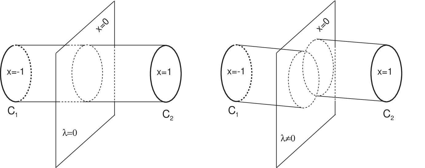
2. For each $a\in{\rm\bf Z}_{k}$, the manifolds $W^{s}_{loc}(\mathcal{P}_{a})$ and $W^{u}_{loc}(\mathcal{P}_{a})$ are smooth surfaces homeomorphic to a cylinder – see Figure 1.

3. For each $a\in{\rm\bf Z}_{k}$, and for $\lambda=0$, one branch of $W^{u}(\mathcal{P}_{a})$ coincides with a branch of $W^{s}(\mathcal{P}_{a+1})$, forming a heteroclinic network, that we call $\Gamma_{0}$, and whose basin of attraction contains an open set.

4. [Transversality] For $\lambda\neq 0$ and for each $a\in{\rm\bf Z}_{k}$, a branch of the two-dimensional manifold $W^{u}(\mathcal{P}_{a})$ intersects transverselly a branch of $W^{s}(\mathcal{P}_{a+1})$ at two trajectories, forming a heteroclinic network $\Gamma_{\lambda}$, consisting of two heteroclinic cycles.

For $\lambda\neq 0$, any one of the two trajectories of (P4) in $W^{u}(\mathcal{P}_{a})\cap W^{s}(\mathcal{P}_{a+1})$ will be denoted $[\mathcal{P}_{a}\to\mathcal{P}_{a+1}]$. A more technical assumption (P5) will be made in Section 4.1 below, after we have established some notation.

For $a\in{\rm\bf Z}_{k}$, define the following constants:

$$\delta_{a}=\frac{c_{a}}{e_{a}}>1,\qquad\mu_{a+1}=\frac{c_{a}}{e_{a+1}}\qquad\text{and}\qquad\delta=\prod_{a=1}^{k}\delta_{a}.$$ (3.3)

Also denote by $\overline{x}_{a}\in{\rm\bf R}^{4}$ the centre of gravity of $\mathcal{P}_{a}$, given by

$$\overline{x}_{a}=\frac{1}{\xi_{a}}\int_{0}^{\xi_{a}}\mathcal{P}_{a}(t)dt\in{\rm\bf R}^{4}.$$

Without loss of generality we assume that the minimal period $\xi_{a}=1$, for all $a\in{\rm\bf Z}_{k}$. It will be explicitly used in system (4.4) below.

3.2 The dynamics

The dynamics of this kind of heteroclinic structures involving periodic solutions has been studied before in [1, 3, 22, 27], in different contexts.

Since $f_{0}$ satisfies (P1)–(P3) then, adapting the Krupa and Melbourne criterion [20, 21], any solution starting sufficiently close to $\Gamma_{0}$ will approach it in positive time; in other words $\Gamma_{0}$ is asymptotically stable. As a trajectory approaches $\Gamma_{0}$, it visits one periodic solution, then moves off to visit the other periodic solutions in the network. After a while it returns to visit the initial periodic solution, and the second visit lasts longer than the first. The oscillatory regime of such a solution seems to switch into different nodes, at geometrically increasing times.

For $\lambda\neq 0$, by (P4), the invariant manifolds of the nodes meet transversally, and the network is no longer asymptotically stable due to the presence of suspended horseshoes in its neighbourhood. As proved in [27], there is an infinite number of heteroclinic and homoclinic connections between any two periodic solutions and the dynamics near the heteroclinic network is very complex. The route to chaos corresponds to an interaction of robust switching with chaotic cycling. The emergence of chaotic cycling does not depend on the magnitude of the multipliers of the periodic solutions. It depends only on the geometry of the flow near the cycle.

In Table 1, we summarise some information about the type of heteroclinic structure of $\Gamma_{\lambda}$ and the type of dynamics nearby.

$\lambda$	Structure of $V_{\Gamma_{\lambda}}$	Dynamics near $\Gamma_{\lambda}$	References
zero	torus of genus $k$	Attractor	[22, 27]
non-zero	torus of genus $>k$	Chaos (Switching and Cycling)	[1, 3, 27]

Table 1: Heteroclinic structure of $\Gamma_{\lambda}$, for $\lambda=0$ and $\lambda\neq 0$.

4 Local and global dynamics near the network

Given a heteroclinic network of periodic solutions $\Gamma_{\lambda}$ with nodes $\mathcal{P}_{a}$, $a\in{\rm\bf Z}_{k}$, let $V_{\Gamma_{\lambda}}$ be a compact neighbourhood of $\Gamma_{\lambda}$ and let $V_{a}$ be pairwise disjoint compact neighbourhoods of the nodes $\mathcal{P}_{a}$, such that each boundary $\partial V_{a}$ is a finite union of smooth manifolds with boundary, that are transverse to the vector field everywhere, except at their boundary. Each $V_{a}$ is called an isolating block for $\mathcal{P}_{a}$ and, topologically, it consists of a hollow cylinder. Topologically, $V_{\Gamma_{0}}$ may be seen as a solid torus with genus $k$ (see Table 1).

4.1 Suspension and local coordinates

For $a\in{\rm\bf Z}_{k}$, let $\Sigma_{a}$ be a cross section transverse to the flow at $p_{a}\in\mathcal{P}_{a}$. Since $\mathcal{P}_{a}$ is hyperbolic, there is a neighbourhood $V^{*}_{a}$ of $p_{a}$ in $\Sigma_{a}$ where the first return map to $\Sigma_{a}$, denoted by $\pi_{a}$, is $C^{1}$ conjugate to its linear part. Moreover, for each $r\geq 2$ there is an open and dense subset of ${\rm\bf R}^{2}$ such that, if the eigenvalues $(c_{a},e_{a})$ lie in this set, then the conjugacy is of class $C^{r}$ — see [32] and Appendix A. The eigenvalues of $d\pi_{a}$ are $e^{e_{a}}$ and $e^{-c_{a}}$. Suspending the linear map gives rise, in cylindrical coordinates $(\rho,\theta,z)$ around $\mathcal{P}_{a}$, to the system of differential equations:

$$\left\{\begin{array}[]{l}\dot{\rho}=-c_{a}(\rho-1)\\ \dot{\theta}=1\\ \dot{z}=e_{a}z\end{array}\right.$$ (4.4)

which is equivalent, after reparametrising the time variable, to the original flow near $\mathcal{P}_{a}$. In these coordinates, the periodic solution $\mathcal{P}_{a}$ is the circle defined by $\rho=1$ and $z=0$, its local stable manifold, $W^{s}_{loc}(\mathcal{P}_{a})$, is the plane defined by $z=0$ and $W^{u}_{loc}(\mathcal{P}_{a})$ is the surface defined by $\rho=1$ as in Figure 1.

Figure 1: Local coordinates on the boundary of the neighbourhood $V_{a}$ of a periodic solution $\mathcal{P}_{a}$ where $a\in{\rm\bf Z}_{k}$. Double bars mean that the sides are identified.

We will work with a hollow three-dimensional cylindrical neighbourhood $V_{a}(\varepsilon)$ of $\mathcal{P}_{a}$ contained in the suspension of $V^{*}_{a}$ given by:

$$V_{a}(\varepsilon)=\left\{(\rho,\theta,z):\quad 1-\varepsilon\leq\rho\leq 1+\varepsilon,\quad-\varepsilon\leq z\leq\varepsilon\quad\text{and}\quad\theta\in{\rm\bf R}\pmod{2\pi}\right\}\ .$$

When there is no ambiguity, we write $V_{a}$ instead of $V_{a}(\varepsilon)$. Its boundary is a disjoint union

$$\partial V_{a}=In(\mathcal{P}_{a})\cup Out(\mathcal{P}_{a})\cup\Omega(\mathcal{P}_{a})$$

such that :

• $In(\mathcal{P}_{a})$ is the union of the walls, defined by $\rho=1\pm\varepsilon$, of the cylinder, locally separated by $W^{u}(\mathcal{P}_{a})$. Trajectories starting at $In(\mathcal{P}_{a})$ go inside the cylinder $V_{a}$ in small positive time.

• $Out(\mathcal{P}_{a})$ is the union of two anuli, the top and the bottom of the cylinder, defined by $z=\pm\varepsilon$, locally separated by $W^{s}(\mathcal{P}_{a})$. Trajectories starting at $Out(\mathcal{P}_{a})$ go inside the cylinder $V_{a}$ in small negative time.

• The vector field is transverse to $\partial V_{a}$ at all points except possibly at the four circles: $\Omega(\mathcal{P}_{a})=\overline{In(\mathcal{P}_{a})}\cap\overline{Out(\mathcal{P}_{a})}$.

The two cylinder walls, $In(\mathcal{P}_{a})$ are parametrised by the covering maps:

$$(\theta,z)\mapsto(1\pm\varepsilon,\theta,z)=(\rho,\theta,z),$$

where $\theta\in\textbf{R}\pmod{2\pi}$, $|z|<\varepsilon$. In these coordinates, $In(\mathcal{P}_{a})\cap W^{s}(\mathcal{P}_{a})$ is the union of the two circles $z=0$. The two anuli $Out(\mathcal{P}_{a})$ are parametrised by the coverings:

$$(\varphi,r)\mapsto(r,\varphi,\pm\varepsilon)=(\rho,\theta,z),$$

for $1-\varepsilon<r<1+\varepsilon$ and $\varphi\in{\rm\bf R}\pmod{2\pi}$ and where $Out(\mathcal{P}_{a})\cap W^{u}(\mathcal{P}_{a})$ is the union of the two circles $r=1$. In these coordinates $\Omega(\mathcal{P}_{a})=\overline{In(\mathcal{P}_{a})}\cap\overline{Out(\mathcal{P}_{a})}$ is the union of the four circles defined by $\rho=1\pm\varepsilon$ and $z=\pm\varepsilon$.

The portion of the unstable manifold of $\mathcal{P}_{a}$ that goes from $\mathcal{P}_{a}$ to $In(\mathcal{P}_{a+1})$ without intersecting $V_{a+1}$ will be denoted $W^{u}_{loc}(\mathcal{P}_{a})$. Similarly, $W^{s}_{loc}(\mathcal{P}_{a})$ will denote the portion of the stable manifold of $\mathcal{P}_{a}$ that is outside $V_{a-1}$ and goes directly from $Out(\mathcal{P}_{a-1})$ to $\mathcal{P}_{a}$. With this notation, we formulate the following technical condition:

1. For $a\in{\rm\bf Z}_{k}$, and $\lambda\neq 0$ close to zero, the manifolds $W^{u}_{loc}(\mathcal{P}_{a})$ intersect the cylinders $In(\mathcal{P}_{a+1})$ on a closed curve. Similarly, $W^{u}_{loc}(\mathcal{P}_{a})$ intersects the annulus $In(\mathcal{P}_{a+1})$ on a closed curve.

The previous hypothesis complements (P4) and corresponds to the expected unfolding from the coincidence of the manifolds $W^{s}(\mathcal{P}_{a+1})$ and $W^{u}(\mathcal{P}_{a})$ at $f_{0}$, see Chilingworth [5]. Note that (P4) and (P5) are satisfied in an open subset of the set of unfoldings $f_{\lambda}$ of $f_{0}$ satisfying (P1)–(P3).

In order to distinguish the local coordinates near the periodic solutions, we sometimes add the index $a$ with $a\in{\rm\bf Z}_{k}$.

4.2 Local map near the periodic solutions

For each $a\in{\rm\bf Z}_{k}$, in the coordinates introduced before, note that the trajectory whose initial condition $(\theta_{a},z_{a})\in In(\mathcal{P}_{a})\backslash W^{s}(\mathcal{P}_{a})$, with $z_{a}>0$, arrives at $Out(\mathcal{P}_{a})$ at time

$$\tau_{a}(\theta_{a},z_{a})=\frac{1}{e_{a}}\ln\left(\frac{\varepsilon}{z_{a}}\right).$$ (4.5)

Integrating (4.4), we may define local maps $\Phi_{a}$ from a connected component of $In(\mathcal{P}_{a})$, with $z_{a}>0$, into a connected component of $Out(\mathcal{P}_{a})$, given by:

$$\Phi_{a}(\theta_{a},z_{a})=\left(\theta_{a}-\frac{1}{e_{a}}\ln\left(\frac{z_{a}}{\varepsilon}\right),1\pm\varepsilon\left(\frac{z_{a}}{\varepsilon}\right)^{\delta_{a}}\right)=(\varphi_{a},r_{a})\qquad\mbox{where}\quad\delta_{a}=\frac{c_{a}}{e_{a}}>1.$$ (4.6)

The signs $\pm$ depend on the component of $In(\mathcal{P}_{a})$ we started at, $+$ for trajectories starting with $r_{a}>1$ and $-$ for $r_{a}<1$. We will discuss the case $r_{a}>1$, $z_{a}>0$, the behaviour on the other components is analogous.

4.3 Flight times for $\lambda=0$

Here we introduce some terminology that will be used in Section 5; see Figure 2. For $X\in\mathcal{B}(\Gamma_{0})$, let $T_{1}(X)$ be the smallest $t\geq 0$ such that $\phi(t,X)\in In(\mathcal{P}_{1})$. For $j\in{\rm\bf N}$, $j>1$, we define $T_{j}(X)$ inductively as the smallest $t>T_{j-1}(X)$ such that $\phi(t,X)\in In(\mathcal{P}_{\langle j\rangle})$, where

$$\left\langle j\right\rangle=j-\left[\frac{j}{k}\right]k$$

is the remainder in the integer division by $k$ and $[x]$ is the greatest integer less than or equal to $x$.

In order to simplify the computations, we may assume that the transition from $Out(\mathcal{P}_{a})$ to $In(\mathcal{P}_{a+1})$ is instantaneous. This is reasonable because, as $t\to\infty$, the time of flight inside each $V_{a}$ tends to infinity, whereas the time of flight from $Out(\mathcal{P}_{a})$ to $In(\mathcal{P}_{a+1})$ remains limited. In the proof of Proposition 1 below, we will see that this assumption does not affect the validity of our results. With this assumption, the time of flight $\tau_{a+nk}(X)$ inside $V_{a}$ at the $n$-th pass of the trajectory through $V_{a}$ will be

$$\tau_{a+nk}(X)=T_{a+1+nk}(X)-T_{a+nk}(X),$$

thus extending the notation $\tau_{a}$ introduced in 4.2 above to $X\in\mathcal{B}(\Gamma_{0})$ and any index $a+nk\in{\rm\bf N}$.

Figure 2: For $X\in\mathcal{B}(\Gamma_{0})$, the solution $\phi(t,X)$ remains in ${V}_{a}$ for a time interval of length $\tau_{a}(X)$, then spends $\tau_{a+1}(X)$ units of time near $\mathcal{P}_{a+1}$, and , after $n$ full turns, stays again in ${V}_{a}$ for $\tau_{a+nk}(X)$ units of time, and so on. The representation is done for $k=3$.

For each $a\in{\rm\bf Z}_{k}$, and for $\lambda=0$, we define the transition map $\Psi_{a}^{0}:Out(\mathcal{P}_{a})\rightarrow In(\mathcal{P}_{a+1})$

$$\Psi_{a}^{0}(\varphi_{a},r_{a})=(\varphi_{a},r_{a}-1)=({\theta}_{a+1},{z}_{a+1}).$$ (4.7)

The transition maps for $\lambda\neq 0$ will be discussed in Section 6.1.

5 The $k$-polygon at the organising centre

Let $f_{0}$ be a vector field in ${\rm\bf R}^{3}$ satisfying (P1)–(P3). All the results of this section assume $\lambda=0$. Suppose, from now on, that $\phi(t,X)$ is a solution $\dot{x}=f_{0}(x)$ with initial condition $X=\phi(0,X)$ in $\mathcal{B}(\Gamma_{0})$, the basin of attraction of $\Gamma_{0}$.

5.1 The statistical limit set of $f_{0}$

The statistical limit set $\Lambda_{stat}(f_{0})$ associated to the basin of attraction of $\Gamma_{0}$ is the smallest closed subset where Lebesgue almost all trajectories spend almost all time. More formally, following Ilyashenko [14] and Karabacak and Ashwin [17], we define:

Definition 2

For an open set $U\subset{\rm\bf R}^{3}$ and a solution $\phi(t,x)$ of (1.1) with $x\in{\rm\bf R}^{3}$:

1. the frequency of the solution being in $U$ is the ratio:

   $$\rho_{f}(x,U,T)=\frac{Leb\{t\in[0,T]:\phi(t,x)\in U\}}{T}.$$

   where $Leb$ denotes the Lebesgue measure in ${\rm\bf R}$.

2. the statistical limit set, denoted by $\Lambda_{stat}({f})$, is the smallest closed subset of ${\rm\bf R}^{3}$ for which any open neighbourhood of $U$ of $\Lambda_{stat}$ satisfies the equality:

   $$\lim_{t\rightarrow+\infty}\rho_{f}(x,U,t)=1,\qquad\text{for almost all }x\in{\rm\bf R}^{3}.$$

Since the transitions between the saddles of $\Gamma_{0}$ are very fast compared with the times of sojourn near the periodic solutions $\mathcal{P}_{a}$, $a\in{\rm\bf Z}_{k}$ (see 4.3) we may conclude that:

Proposition 1

Let $f_{0}$ be a vector field in ${\rm\bf R}^{3}$ satisfying (P1)–(P3). Then:

$$\Lambda_{stat}({f_{0}})=\bigcup_{a=1}^{k}\mathcal{P}_{a}\subset\Gamma_{0}.$$

Proof: The flow from $Out(\mathcal{P}_{a})$ to $In(\mathcal{P}_{a+1})$ is non-singular as in a flow-box. Since both $Out(\mathcal{P}_{a})$ and $In(\mathcal{P}_{a+1})$ are compact sets, the time of flight between them has a positive maximum. On the other hand, for each $a\in{\rm\bf Z}_{k}$, the time of flight inside $V_{a}$ from $In(\mathcal{P}_{a})\backslash W^{s}_{loc}(\mathcal{P}_{a})$ to $Out(\mathcal{P}_{a})$ tends to infinity as $t$ approach the stable manifold of $\mathcal{P}_{a}$, $W^{s}_{loc}(\mathcal{P}_{a})$, or equivalently as the trajectory accumulates on $\Gamma_{0}$.

Remark 1

It follows from Proposition 1 that, for each $a\in{\rm\bf Z}_{k}$, the time intervals in which trajectories are travelling from $Out(\mathcal{P}_{a})$ to $In(\mathcal{P}_{a+1})$ do not affect the accumulation points of the time averages of a solution that is accumulating on $\Gamma_{0}$. This result will be useful in the proof of the Theorem 10 because it shows that the duration of the journeys between nodes may be statistically neglected.

5.2 Estimates of flight times

In this section, we obtain relations between flight times of a trajectory in consecutive isolating blocks as well as other estimates that will be used in the sequel.

Lemma 2

For all $j\in{\rm\bf N}$ and any initial condition $X\in\mathcal{B}(\Gamma_{0})$ we have:

$$\frac{\tau_{j+1}(X)}{\tau_{j}(X)}=\frac{c_{\langle j\rangle}}{e_{\langle j+1\rangle}}.$$ (5.8)

In particular the ratio ${\tau_{j+1}(X)}/{\tau_{j}(X)}$ does not depend on $X$.

Proof: Given $j\in{\rm\bf N}$, let $X_{j}=\left(\theta_{j},z_{j}\right)=\phi\left(T_{j}(X),X\right)\in In(\mathcal{P}_{\langle j\rangle})$. Using the expressions (4.5), (4.6) and the expression for $\Psi_{\langle j\rangle}^{0}$ in (4.7), we have:

$$\tau_{j+1}(X)=\frac{1}{e_{\langle j+1\rangle}}\ln\left(\frac{\varepsilon}{\varepsilon\left(\frac{z_{j}}{\varepsilon}\right)^{\delta_{\langle j\rangle}}}\right)=\frac{1}{e_{\langle j+1\rangle}}\delta_{\langle j\rangle}\left[\ln(\varepsilon)-\ln(z_{j})\right]$$

Thus

$$\frac{\tau_{j+1}(X)}{\tau_{j}(X)}=\frac{\frac{1}{e_{\langle j+1\rangle}}\delta_{\langle j\rangle}\left[\ln(\varepsilon)-\ln(z_{j})\right]}{\frac{1}{e_{\langle j\rangle}}\left[\ln(\varepsilon)-\ln(z_{j})\right]}=\frac{e_{\langle j\rangle}}{e_{\langle j+1\rangle}}\delta_{\langle j\rangle}=\frac{c_{\langle j\rangle}}{e_{\langle j+1\rangle}}.$$

Recall from (3.3) that $\displaystyle\mu_{a+1}=\frac{c_{a}}{e_{a+1}}$, $a\in{\rm\bf Z}\pmod{k}$. With this notation we obtain:

Corollary 3

For $i,j\in{\rm\bf N}$ such that $j>i>1$, and for any $X\in\mathcal{B}(\Gamma_{0})$, we have:

1. $\frac{\tau_{j+k}(X)}{\tau_{j}(X)}=\prod_{a=1}^{k}\mu_{a+1}=\prod_{j=1}^{k}\delta_{j}=\delta>1$.

2. $\tau_{j+1}(X)=\tau_{i}(X)\prod^{j+1}_{l=i+1}\mu_{\langle l\rangle}$.

Lemma 4

For $a\in{\rm\bf Z}_{k}$, and for any $X\in\mathcal{B}(\Gamma_{0})$, the following equalities hold:

1. $T_{a+nk}(X)=T_{a}(X)+\frac{\delta^{n}-1}{\delta-1}\left(\mu_{a}+\mu_{a}\mu_{a+1}+\ldots+\prod_{l=0}^{k-1}\mu_{a+l}\right)\tau_{a-1}(X);$

2. $\tau_{a+nk}(X)=T_{a+1+nk}(X)-T_{a+nk}(X)=\delta^{n}\mu_{a}\tau_{a-1}(X)$.

Proof:

1. If $n=0$ ($n$ corresponds to the number of loops around the cycle $\Gamma_{0}$), it is trivial. For $n\geq 1$, we may write the following equality, omitting the dependence on $X$:

   $$T_{a+nk}= T_{a} +\quad\tau_{a}+\tau_{a+1}+\ldots\tau_{a+k-1}+$$

   $$+\quad\tau_{a+k}+\tau_{a+k+1}+\ldots\tau_{a+2k-1}+\ldots$$

   $$+\quad\tau_{a+(n-1)k}+\tau_{a+(n-1)k+1}+\ldots\tau_{a+nk-1}$$

   Using Corollary 3, the previous equality yields:

   $$T_{a+nk}= T_{a} +\mu_{a}\tau_{a-1}+\mu_{a}\mu_{a+1}\tau_{a-1}+\ldots\prod_{l=0}^{k-1}\mu_{a+l}\tau_{a-1}+$$

   $$+\delta\mu_{a}\tau_{a-1}+\delta\mu_{a}\mu_{a+1}\tau_{a-1}+\ldots\delta\left(\prod_{l=0}^{k-1}\mu_{a+l}\right)\tau_{a-1}+\ldots$$

   $$+\delta^{n-1}\mu_{a}\tau_{a-1}+\delta^{n-1}\mu_{a}\mu_{a+1}\tau_{a-1}+\ldots\delta^{n-1}\left(\prod_{l=0}^{k-1}\mu_{a+l}\right)\tau_{a-1}=$$

   $$= T_{a} +\frac{\delta^{n}-1}{\delta-1}\left(\mu_{a}+\mu_{a}\mu_{a+1}+\ldots+\prod_{l=0}^{k-1}\mu_{a+l}\right)\tau_{a-1}$$

2. This item follows from Corollary 3. Indeed, we have:

   $$\tau_{a+nk}(X)=\mu_{a}\tau_{a+nk-1}(X)=\mu_{a}\mu_{a-1}\tau_{a+nk-2}(X)=\ldots=\delta^{n}\tau_{a}(X)=\delta^{n}\mu_{a}\tau_{a-1}(X).$$

5.3 The vertices of the $k$-polygon

In this section, we show that in $\mathcal{B}(\Gamma_{0})$ the time averages fail to converge, by finding several accumulation points for them. For each $a\in{\rm\bf Z}_{k}$, define the point

$$A_{a}=\frac{\overline{x}_{a}+\mu_{a+1}\overline{x}_{a+1}+\mu_{a+1}\mu_{a+2}\overline{x}_{a+2}+\ldots+\prod_{l=1}^{k-1}\mu_{a+l}\overline{x}_{a+k-1}}{1+\mu_{a+1}+\mu_{a+1}\mu_{a+2}+\ldots+\prod_{l=1}^{k-1}\mu_{a+l}}=\frac{num(A_{a})}{den(A_{a})}$$ (5.9)

Note that $A_{a}$ and $num(A_{a})$ lie in ${\rm\bf R}^{4}$ and $den(A_{a})\in{\rm\bf R}$. Later we will see that these points are the vertices of a polygon of accumulation points. First we show that they are accumulation points for the time averages.

Proposition 5

Let $a\in{\rm\bf Z}_{k}$, let $f_{0}$ be a vector field in ${\rm\bf R}^{3}$ satisfying (P1)–(P3) and let $\phi(t,X)$ a solution of $\dot{x}=f_{0}(x)$ with $X\in\mathcal{B}(\Gamma_{0})$. Then

$$\lim_{n\rightarrow+\infty}\left[\frac{1}{T_{a+nk}}\int_{0}^{T_{a+nk}}\phi(t,X)dt\right]=A_{a}$$

We divide the proof in two lemmas. First we show in Lemma 6 that it is sufficient to consider the limit when $n\to\infty$ of the averages over one turn around $\Gamma_{0}$. Then in Lemma 7 we show that these averages tend to $A_{a}$.

Lemma 6

Let $T_{\ell}$, $\ell\in{\rm\bf N}$ be a sequence $0=T_{0}<T_{\ell}<T_{\ell+1}$ with $\lim_{\ell\to\infty}T_{\ell}=\infty$. Given $g:{\rm\bf R}\rightarrow{\rm\bf R}^{m}$ an integrable map,

$$\mbox{if }\lim_{\ell\to\infty}\frac{1}{T_{\ell+1}-T_{\ell}}\int_{T_{\ell}}^{T_{\ell+1}}g(t)dt=\omega,\qquad\mbox{then}\qquad\lim_{\ell\to\infty}\frac{1}{T_{\ell}}\int_{0}^{T_{\ell}}g(t)dt=\omega.$$

Proof: First note that

$$\frac{1}{T_{\ell}}\int_{0}^{T_{\ell}}g(t)dt-\omega=\frac{1}{T_{\ell}}\int_{0}^{T_{\ell}}(g(t)-\omega dt=\sum_{j=1}^{\ell}\left(\frac{T_{j}-T_{j-1}}{T_{\ell}}\right)\left[\frac{1}{T_{j}-T_{j-1}}\int_{T_{j-1}}^{T_{j}}(g(t)-\omega)dt\right].$$

From the hypothesis, given $\varepsilon>0$ there exists $N_{1}$ such that $\ell>N_{1}$ implies

$$\frac{1}{T_{\ell}-T_{\ell-1}}\left|\int_{T_{\ell-1}}^{T_{\ell}}(g(t)-\omega)dt\right|<\frac{\varepsilon}{2}.$$

Let $A=\displaystyle\left|\int_{0}^{T_{N_{1}}}(g(t)-\omega)dt\right|$. Since $T_{\ell}\to\infty$ then there exists $N_{2}$ such that $T_{N_{2}}>2A/\varepsilon$. Let $N_{0}=\max\left\{N_{1},N_{2}\right\}$. If $\ell>N_{0}$ then

$$\left|\frac{1}{T_{\ell}}\int_{0}^{T_{\ell}}(g(t)-\omega)dt\right| \leq \frac{1}{T_{\ell}}\left|\int_{0}^{T_{N_{1}}}(g(t)-\omega)dt\right|+\frac{1}{T_{\ell}}\left|\int_{T_{N_{1}}}^{T_{\ell}}(g(t)-\omega)dt\right|$$

$$\leq \frac{A}{T_{\ell}}+\sum_{j=N_{1}}^{\ell}\left(\frac{T_{j}-T_{j-1}}{T_{\ell}}\right)\ \frac{1}{T_{j}-T_{j-1}}\left|\int_{T_{j-1}}^{T_{j}}(g(t)-\omega)dt\right|$$

$$\leq \frac{\varepsilon}{2}+\sum_{j=N_{1}}^{\ell}\left(\frac{T_{j}-T_{j-1}}{T_{\ell}}\right)\frac{\varepsilon}{2}\leq\frac{\varepsilon}{2}\left(1+\sum_{j=1}^{\ell}\frac{T_{j}-T_{j-1}}{T_{\ell}}\right)=\varepsilon.$$

Lemma 7

Let $f_{0}$ be a vector field in ${\rm\bf R}^{3}$ satisfying (P1)–(P3). For each $a\in{\rm\bf Z}_{k}$, and for each $X\in\mathcal{B}(\Gamma_{0})$, the limit of the spatial average of of $\phi(t,X)$ over one full turn around the heteroclinic cycle $\Gamma_{0}$ starting at $In(\mathcal{P}_{j})$ is $A_{j}$. More precisely:

$$\lim_{n\to\infty}\frac{1}{T_{a+(n+1)k}(X)-T_{a+nk}(X)}\int_{T_{a+(n+1)k}(X)}^{T_{a+nk}(X)}\phi(t,X)dt=A_{a}.$$

Proof: First, recall that we are assuming that, for all $a\in{\rm\bf Z}_{k}$, the jumps from $Out(\mathcal{P}_{a})$ to $In(\mathcal{P}_{a+1})$ are instantaneous (see Remark 1). Since $X\in\mathcal{B}(\Gamma_{0})$, then for $t\in\left[T_{a+nk},T_{a+1+nk}\right]$ with large $n$, the trajectory $\phi(t,X)$ gets very close to $\mathcal{P}_{a}$. Therefore, omitting the $(X)$ for shortness, we have:

$$\lim_{n\to\infty}\frac{1}{T_{a+1+nk}-T_{a+nk}}\int_{T_{a+nk}}^{T_{a+1+nk}}\phi(t,X)dt=\lim_{n\to\infty}\frac{1}{\tau_{a+nk}}\int_{T_{a+nk}}^{T_{a+1+nk}}\phi(t,X)dt=\overline{x_{a}}.$$ (5.10)

Without loss of generality, from now on we take $a=1$. Then

$$\frac{1}{T_{k+1+nk}-T_{1+nk}}\int_{T_{1+nk}}^{T_{k+1+nk}}\phi(t,X)dt$$

$$= \frac{1}{T_{k+1+nk}-T_{1+nk}}\left[\int_{T_{1+nk}}^{T_{2+nk}}\phi(t,X)dt+\int_{T_{2+nk}}^{T_{3+nk}}\phi(t,X)dt+\cdots+\int_{T_{k+nk}}^{T_{k+1+nk}}\phi(t,X)dt\right]$$

$$= \sum_{b=1}^{k}\frac{T_{b+1+nk}-T_{b+nk}}{T_{k+1+nk}-T_{1+nk}}\left[\frac{1}{T_{b+1+nk}-T_{b+nk}}\int_{T_{b+nk}}^{T_{b+1+nk}}\phi(t,X)dt\right].$$

Recall that $T_{2+nk}-T_{1+nk}=\tau_{1+nk}$, and by Corollary 3, for any $b\in\{2,\ldots,k\}$

$$\frac{T_{b+1+nk}-T_{b+nk}}{T_{k+1+nk}-T_{1+nk}} = \frac{\tau_{b+nk}}{\tau_{1+nk}+\tau_{2+nk}+\ldots+\tau_{k+nk}}$$

$$= \frac{\mu_{b}\mu_{b-1}\ldots\mu_{2}\tau_{1+nk}}{\tau_{1+nk}+\mu_{2}\tau_{1+nk}+\ldots+\mu_{k}\mu_{k-1}\ldots\mu_{2}\tau_{1+nk}}$$

$$= \frac{\mu_{b}\mu_{b-1}\ldots\mu_{2}}{denA_{1}}.$$

Therefore, the value of

$$\lim_{n\rightarrow+\infty}\frac{1}{T_{k+1+nk}-T_{1+nk}}\int_{T_{1+nk}}^{T_{k+1+nk}}\phi(t,X)dt$$

is, by (5.10),

$$\lim_{n\rightarrow+\infty}\frac{1}{denA_{1}}\left[\frac{1}{T_{2+nk}-T_{1+nk}}\int_{T_{1+nk}}^{T_{2+nk}}\phi(t,X)dt+\sum_{b=2}^{k}\frac{\mu_{b}\mu_{b-1}\ldots\mu_{2}}{T_{b+1+nk}-T_{b+nk}}\int_{T_{b+nk}}^{T_{b+1+nk}}\phi(t,X)dt\right]$$

$$= \frac{\overline{x}_{1}+\mu_{2}\overline{x}_{2}+\ldots+\mu_{k}\mu_{k-1}\ldots\mu_{2}\overline{x}_{k}}{1+\mu_{2}+\ldots+\mu_{k}\mu_{k-1}\ldots\mu_{2}}=A_{1}.$$

5.4 The sides of the $k$-polygon

In Section 5.3 we have shown that for $a\in{\rm\bf Z}\pmod{k}$, the time average over the sequences $T_{a+nk}$ of times accumulate, as $n\to\infty$ in the $A_{a}$. In this section we describe accumulation points for intermediate sequences of times $t_{n}$. For this, it will be useful to know how $A_{a}$ and $A_{a+1}$ are related:

Lemma 8

For all $a\in{\rm\bf Z}\pmod{k}$, the following equalities hold:

$$\mu_{a+1}den(A_{a+1})=den(A_{a})-(1-\delta)\qquad\mbox{and}\qquad\mu_{a+1}num(A_{a+1})=num(A_{a})-(1-\delta)\overline{x}_{a}.$$ (5.11)

Proof: Expanding $den(A_{a})$ and $den(A_{a+1})$, yields:

$$den(A_{a})={1+\mu_{a+1}+\mu_{a+1}\mu_{a+2}+\cdots+\prod_{l=1}^{k-1}\mu_{l+a}}\qquad den(A_{a+1})={1+\mu_{a+2}+\mu_{a+2}\mu_{a+2}+\cdots+\prod_{l=1}^{k-1}\mu_{l+a+1}}$$

hence, since $\prod_{l=0}^{k-1}\mu_{l+a+1}=\delta$,

$$\mu_{a+1}den(A_{a+1}) = {\mu_{a+1}+\mu_{a+1}\mu_{a+2}+\mu_{a+1}\mu_{a+2}\mu_{a+2}+\cdots+\mu_{a+1}\prod_{l=1}^{k-1}\mu_{l+a+1}}$$

$$= \mu_{a+1}+\mu_{a+1}\mu_{a+2}+\mu_{a+1}\mu_{a+2}\mu_{a+2}+\cdots+\prod_{l=1}^{k-1}\mu_{l+a}+\delta$$

$$= den(A_{a})-(1-\delta).$$

For $num(A_{a})$ and $num(A_{a+1})$ we obtain

$$num(A_{a})=\overline{x}_{a}+\mu_{a+1}\overline{x}_{a+1}+\mu_{a+1}\mu_{a+2}\overline{x}_{a+2}+\cdots+\left(\prod_{l=1}^{k-1}\mu_{l+a}\right)\overline{x}_{a+k-1}$$

$$num(A_{a+1})=\overline{x}_{a+1}+\mu_{a+2}\overline{x}_{a+2}+\mu_{a+2}\mu_{a+3}\overline{x}_{a+3}+\cdots+\left(\prod_{l=1}^{k-1}\mu_{l+a+1}\right)\overline{x}_{a+k}$$

and, since $\overline{x}_{a+k}=\overline{x}_{a}$, we get

$$\mu_{a+1}num(A_{a+1}) = \mu_{a+1}\overline{x}_{a+1}+\mu_{a+1}\mu_{a+2}\overline{x}_{a+2}+\mu_{a+1}\mu_{a+2}\mu_{a+3}\overline{x}_{a+3}+\cdots+\mu_{a+1}\left(\prod_{l=1}^{k-1}\mu_{l+a+1}\right)\overline{x}_{a+k}$$

$$= \mu_{a+1}\overline{x}_{a+1}+\mu_{a+1}\mu_{a+2}\overline{x}_{a+2}+\mu_{a+1}\mu_{a+2}\mu_{a+3}\overline{x}_{a+3}+\cdots+\left(\prod_{l=1}^{k-1}\mu_{l+a}\right)\overline{x}_{a+k-1}+\delta\overline{x}_{a}$$

$$= num(A_{a})-(1-\delta)\overline{x}_{a}$$

and the lemma is proved.

Proposition 9

If $f_{0}$ is a vector field in ${\rm\bf R}^{3}$ satisfying (P1)–(P3), then for each $a\in{\rm\bf Z}_{k}$ the point $A_{a+1}$ lies in the segment connecting $A_{a}$ to $\overline{x}_{a}$.

Proof: We use Lemma 8 to obtain

$$num(A_{a+1})=\frac{1}{\mu_{a+1}}num(A_{a})+\frac{\delta-1}{\mu_{a+1}}\overline{x}_{a}$$

and hence

$$A_{a+1}=\frac{num(A_{a+1})}{den(A_{a+1})}=\left(\frac{den(A_{a})}{\mu_{a+1}den(A_{a+1})}\right)\frac{num(A_{a})}{den(A_{a})}+\left(\frac{\delta-1}{\mu_{a+1}den(A_{a+1})}\right)\overline{x}_{a}=\alpha A_{a}+\beta\overline{x}_{a}.$$

Again from Lemma 8 we have $den(A_{a})=\mu_{a+1}den(A_{a+1})-(\delta-1)$, and therefore

$$\alpha=\frac{den(A_{a})}{\mu_{a+1}den(A_{a+1})}=1-\frac{\delta-1}{\mu_{a+1}den(A_{a+1})}=1-\beta$$

hence $A_{a+1}$ lies in the line through $A_{a}$ and $\overline{x}_{a}$. From the expression in Lemma 8 it follows that $\mu_{a+1}den(A_{a+1})-den(A_{a})=\delta-1<0$, hence $0<\alpha<1$ and thus $A_{a+1}$ lies in the segment from $A_{a}$ to $\overline{x}_{a}$, proving the result.

Figure 3: Representation of the sequence of times $\lambda_{n}\tau_{a+nk}$, where $a\in{\rm\bf Z}_{k}$, is fixed and $n\in{\rm\bf N}$.

We now come to the main result of this section:

Theorem 10

If $f_{0}$ is a vector field in ${\rm\bf R}^{3}$ satisfying (P1)–(P3), then for any $X\in\mathcal{B}(\Gamma_{0})$, the set of accumulation points of the time average $\frac{1}{T}\int_{0}^{T}\phi(t,X)dt$ is the boundary of the $k$-polygon defined by $A_{1},\ldots,A_{k}\in{\rm\bf R}^{3}$. Moreover, when $\delta\rightarrow 1$ the polygon collapses into a point.

Proof: First we show that all points in the boundary of the polygon are accumulation points. Given $L\in[0,1]$ and $a\in{\rm\bf Z}_{k}$, consider the sequence $t_{n}=T_{a+nk}+L\tau_{a+nk}$, we want the accumulation points of $\mathcal{L}_{n}=\frac{1}{t_{n}}\int_{0}^{t_{n}}\phi(t,X)dt$ as $n\to\infty$. For this we write

$$\mathcal{L}_{n}=\frac{1}{t_{n}}\int_{0}^{t_{n}}\phi(t,X)dt = \frac{1}{t_{n}}\int_{0}^{T_{a+nk}}\phi(t,X)dt+\frac{1}{t_{n}}\int_{T_{{a+nk}}}^{t_{n}}\phi(t,X)dt$$

$$= \alpha_{n}\left(\frac{1}{T_{{a+nk}}}\int_{0}^{T_{a+nk}}\phi(t,X)dt\right)+\beta_{n}\left(\frac{1}{t_{n}-T_{{a+nk}}}\int_{T_{{a+nk}}}^{t_{n}}\phi(t,X)dt\right),$$

where

$$0<\alpha_{n}=\frac{T_{a+nk}}{t_{n}}\leq 1\qquad 0\leq\beta_{n}=\frac{t_{n}-T_{{a+nk}}}{t_{n}}\leq 1\qquad\alpha_{n}+\beta_{n}=1.$$

Since both $\alpha_{n}$ and $\beta_{n}$ are limited, each one of them contains a converging subsequence. We analyse separately each of the terms in the expression for $\mathcal{L}_{n}$ above.

We have already seen in Proposition 5 that, if $X\in\mathcal{B}(\Gamma_{0})$, then $\lim_{n\to\infty}\frac{1}{T_{a+nk}}\int_{0}^{T_{a+nk}}\phi(t,X)dt=A_{a}$. In particular, if $L=0$, then $\alpha_{n}=1$, $\beta_{n}=0$ and $\lim_{n\to\infty}\mathcal{L}_{n}=A_{a}$.

We claim that if $L\neq 0$, then $\lim_{n\to\infty}\frac{1}{t_{n}-T_{a+nk}}\int_{T_{{a+nk}}}^{t_{n}}\phi(t,X)dt=\overline{x}_{a}$. To see this, note that $\phi(t,X)\in V_{a}$ for $t\in[T_{a+nk},t_{n}]$. Moreover, since $\lim_{n\to\infty}\tau_{a+nk}=\infty$, then for large $n$, we have that $t_{n}-T_{a+nk}=L\tau_{a+nk}$ is much larger than $\xi_{a}$, the period of $\mathcal{P}_{a}$. Since $X\in\mathcal{B}(\Gamma_{0})$, then $\phi(t,X)$, with $t\in[T_{a+nk},t_{n}]$, tends to $\mathcal{P}_{a}$ when $n\to\infty$ and the average of $\phi(t,X)$ tends to $\overline{x}_{a}$, the average of $\mathcal{P}_{a}$.

At this point we have established that any accumulation point of $\mathcal{L}_{n}$ lies in the segment connecting $A_{a}$ to $\overline{x}_{a}$. We have shown in Proposition 9 that this segment also contains $A_{a+1}$. By Proposition 5 we have that $\lim_{n\to\infty}\mathcal{L}_{n}=A_{a+1}$ for $L=1$. On the other hand, $\beta_{n}$ is an increasing function of $L$, so, as $L$ increases from 0 to 1, the accumulation points of $\mathcal{L}_{n}$ move from $A_{a}$ to $A_{a+1}$ in the segment connecting them.

Conversely, any accumulation point lies on the boundary of the polygon. To see this, let $A$ be an accumulation point of the time average. This means that there is an increasing sequence of times $s_{n}$, tending to infinity, and such that $\lim_{n\to\infty}\mathcal{L}_{n}=A$, where $\mathcal{L}_{n}=\frac{1}{s_{n}}\int_{0}^{s_{n}}\phi(t,x)dt$. Since $s_{n}$ tends to infinity, then it may be partitioned into subsequences of the form $s_{n_{j}}=T_{a+n_{j}k}+L_{n_{j}}\tau_{a+n_{j}k}$ for each $a\in{\rm\bf Z}_{k}$, and some $L_{n_{j}}\in[0,1]$. The arguments above, applied to this subsequence, show that the accumulation points of $\mathcal{L}_{n_{j}}$ lie in the segment connecting $A_{a}$ to $A_{a+1}$. Therefore, since $\mathcal{L}_{n}$ converges, there are two possibilities. The first is that all the $s_{n}$ (except possibly finitely many) are of the form above for a fixed $a\in{\rm\bf Z}_{k}$, and hence $A$ lies in the the segment connecting $A_{a}$ to $A_{a+1}$. The second possibility is that all the $s_{n}$ (except maybe a finite number) are of one of the forms $s_{n_{j}}=T_{a+n_{j}k}+L_{n_{j}}\tau_{a+n_{j}k}$ or $s_{n_{i}}=T_{a+1+n_{i}k}+L_{n_{i}}\tau_{a+1+n_{i}k}$, and that $A=A_{a+1}$. In both cases, the accumulation point of the time average will lie on the boundary of the polygon.

Finally, when $\delta\to 1$, the expressions (5.11) in Lemma 8 become $\mu_{a+1}den(A_{a+1})=den(A_{a})$ and $\mu_{a+1}num(A_{a+1})=num(A_{a})$, hence

$$A_{a}=\frac{num(A_{a})}{den(A_{a})}=\frac{\mu_{a+1}num(A_{a+1})}{\mu_{a+1}den(A_{a+1})}=A_{a+1}$$

and the polygon collapses to a point at the same time as $\Gamma_{0}$ stops being attracting.

Figure 4: The polygon in Theorem 10 with $k=3$: the accumulation points of the time average $\frac{1}{T}\int_{0}^{T}\phi(t,x)dt$ lie on the boundary of the triangle defined by $A_{1},A_{2}$ and $A_{3}.$

Corollary 11

If $f_{0}$ is a vector field in ${\rm\bf R}^{3}$ satisfying (P1)–(P3), then all points in the basin of attraction of $\Gamma_{0}$ have historic behaviour. In particular the set of initial conditions with historic behaviour has positive Lebesgue measure.

The points of $\Gamma_{0}$ do not have historic behaviour. Indeed, if $X\in\Gamma_{0}$ then either $X\in\mathcal{P}_{a}$ or $\phi(t,X)$ accumulates on $\mathcal{P}_{a}$ for some $a\in\{1,\ldots,k\}$. In both cases, $\lim_{T\to\infty}\frac{1}{T}\int_{0}^{T}\phi(t,X)dt=\overline{x}_{a}$.

The previous proofs have been done for a piecewise continuous trajectory; when $t=T_{a}$, the trajectory jumps from $V_{a-1}$ to $V_{a}$, whereas the real solutions have a continuous motion from $V_{a-1}$ to $V_{a}$ along the corresponding heteroclinic connection, during a bounded interval of time. As shown in Proposition 1, the statistical limit set of $\Gamma_{0}$ is $\bigcup_{a=1}^{k}\mathcal{P}_{a}$ meaning that trajectories spend Lebesgue almost all time near the periodic solutions, and not along the connections. Therefore, the intervals in which the transition occurs do not affect the accumulation points of the time averages of the trajectories and the result that was shown for a piecewise continuous trajectory holds.

6 Persistence of historic behaviour

From now on, we discuss he differential equation $\dot{x}=f_{\lambda}(x)$ satisfying (P1)–(P5), with $\lambda\neq 0$. In this case it was shown in Rodrigues et al [27] that the simple dynamics near $\Gamma_{0}$ jumps to chaotic behaviour near $\Gamma_{\lambda}$.

6.1 Invariant manifolds for $\lambda>0$

Figure 5: For $\lambda$ close to zero, both $W^{s}_{loc}(\mathcal{P}_{a+1})\cap Out(\mathcal{P}_{a})$ and $W^{u}_{loc}(\mathcal{P}_{a})\cap In(\mathcal{P}_{a+1})$ are closed curves, given in local coordinates as the graphs of periodic functions; this is the expected unfolding from the coincidence of the invariant manifolds at $\lambda=0$.

We describe the geometry of the two-dimensional local invariant manifolds of $\mathcal{P}_{a}$ and $\mathcal{P}_{a+1}$ for $\lambda\neq 0$, under the assumptions (P1)–(P5).

For this, let $f_{\lambda}$ be an unfolding of $f_{0}$ satisfying (P1)–(P5). For $\lambda\neq 0$, we introduce the notation:

• $(O_{a}^{1},0)$ and $(O_{a}^{2},0)$ with $0<O_{a}^{1}<O_{a}^{2}<2\pi$ are the coordinates of the two points where the connections $[\mathcal{P}_{a}\rightarrow\mathcal{P}_{a+1}]$ of Properties (P4)–(P5) meet $Out(\mathcal{P}_{a})$;

• $(I_{a}^{1},0)$ and $(I_{a}^{2},0)$ with $0<I_{a}^{1}<I_{a}^{2}<2\pi$ are the coordinates of the two points where $[\mathcal{P}_{a-1}\rightarrow\mathcal{P}_{a}]$ meets $In(\mathcal{P}_{a})$;

• $(O_{a}^{i},0)$ and $(I_{a+1}^{i},0)$ are on the same trajectory for each $i\in\{1,2\}$ and $a\in{\rm\bf Z}_{k}$.

By (P5), for small $\lambda>0$, the curves $W^{s}_{loc}(\mathcal{P}_{a+1})\cap Out(\mathcal{P}_{a})$ and $W^{u}_{loc}(\mathcal{P}_{a})\cap In(\mathcal{P}_{a+1})$ can be seen as graphs of smooth periodic functions, for which we make the following conventions (see Figure 5):

• $W^{s}_{loc}(\mathcal{P}_{a+1})\cap Out(\mathcal{P}_{a})$ is the graph of $y=g_{a}^{\lambda}(\varphi)$, with $g_{a}^{\lambda}(O_{a}^{i})=1$, for $i\in\{1,2\}$ and $a\in{\rm\bf Z}_{k}$.

• $W^{u}_{loc}(\mathcal{P}_{a-1})\cap In(\mathcal{P}_{a})$ is the graph of $y=h_{a}^{\lambda}(\theta)$, with $h_{a}^{\lambda}(I_{a}^{i})=0$, for $i\in\{1,2\}$ and $a\in{\rm\bf Z}_{k}$.

• omitting the superscript $\lambda$, we have: $h_{a}^{\prime}(I_{a}^{1})>0$, $h_{a}^{\prime}(I_{a}^{2})<0$, $g_{a}^{\prime}(O_{a}^{2})>0$ and $g_{a}^{\prime}(O_{a}^{1})<0$, for $i\in\{1,2\}$.

The two points $(O_{a}^{1},0)$ and $(O_{a}^{2},0)$ divide the closed curve $W^{s}_{loc}(\mathcal{P}_{a+1})\cap Out(\mathcal{P}_{a})$ in two components, corresponding to different signs of $r_{a}-1$. With the conventions above, we get $g_{a}^{\lambda}(\varphi)>1$ for $\varphi\in\left(O_{a}^{2},O_{a}^{1}\right)$. More specifically, the region in $Out(\mathcal{P}_{a})$ between $W_{loc}^{s}(\mathcal{P}_{a+1})$ and $W_{loc}^{u}(\mathcal{P}_{a})$ given by

$$A=\{(\varphi_{a},r_{a})\in Out(\mathcal{P}_{a}):1<r_{a}<g_{a}^{\lambda}(\varphi_{a})\}$$

is mapped by $\Psi_{a}$ into the lower ($z_{a}<0$) part of $In(\mathcal{P}_{a+1})$. Similarly, the region

$$B=\{(\varphi_{a},r_{a})\in Out(\mathcal{P}_{a}):r_{a}>1\}\backslash A=\{(\varphi_{a},r_{a})\in Out(\mathcal{P}_{a}):1<r_{a}\ \mbox{ and }\ g_{a}^{\lambda}(\varphi_{a})<r_{a}\}$$

(see Figure 6) is mapped into the $z_{a}>0$ component of $In(\mathcal{P}_{a+1})$.

Figure 6: The component $A$ of $Out(\mathcal{P}_{a})$ between $W_{loc}^{s}(\mathcal{P}_{a+1})$ and $W_{loc}^{u}(\mathcal{P}_{a})$ is mapped by $\Psi_{a}$ into the lower ($z_{a+1}<0$) part of $In(\mathcal{P}_{a+1})$, its complement $B$ in the $r_{a}>1$ component of $Out(\mathcal{P}_{a})$ is mapped by $\Psi_{a}$ into the upper ($z_{a+1}>0$) part of $In(\mathcal{P}_{a+1})$.

The maximum value of $g_{a}^{\lambda}(\varphi)$ is attained at some point

$$(\varphi_{a},r_{a})=(\varphi_{a}^{O}(\lambda),M_{a}^{O}(\lambda))\qquad\text{with}\qquad O_{a}^{2}<\varphi_{a}^{O}(\lambda)<O_{a}^{1}.$$

We denote by $M^{I}_{a}(\lambda)$ the maximum value of $h_{a}^{\lambda}$.

6.2 Geometrical preliminaries

We will need to introduce some definitions.

Figure 7: A spiral is defined on a covering of the annulus $Out(\mathcal{P}_{a})$ by a smooth curve that turns around the annulus infinitely many times as its radius tends to $\nu\in[0,1]$. It contains a fold point and a point of maximum radius.

Definition 3

A spiral on the annulus $\mathcal{A}$ accumulating on the circle $r=\nu$ is a curve on $\mathcal{A}$, without self-intersections, that is the image, by the parametrisation $(\varphi,r)$ of the annulus, of a continuous map $H:(b,c)\rightarrow{\rm\bf R}\times[0,1]$,

$$H(s)=\left(\varphi(s),r(s)\right),$$

such that:

1. there are $\tilde{b}\leq\tilde{c}\in(b,c)$ for which both $\varphi(s)$ and $r(s)$ are monotonic in each of the intervals $(b,\tilde{b})$ and $(\tilde{c},c)$;

2. either $\lim_{s\to b^{+}}\varphi(s)=\lim_{s\to c^{-}}\varphi(s)=+\infty$ or $\lim_{s\to b^{+}}\varphi(s)=\lim_{s\to c^{-}}\varphi(s)=-\infty,$

3. $\lim_{s\to b^{+}}r(s)=\lim_{s\to c^{-}}r(s)=\nu$.

It follows from the assumptions on the function $\varphi(s)$ that it has either a global minimum or a global maximum, and that $r(s)$ always has a global maximum. The point where the map $\varphi(s)$ has a global minimum or a global maximum will be called a fold point of the spiral. The global maximum value of $r(s)$ will be called the maximum radius of the spiral.

6.3 Geometry of the transition maps $\Phi_{a}$

Proposition 12

Under the conventions of Section 6.1, for each $a\in{\rm\bf Z}_{k}$, the local map $\Phi_{a}$ transforms the part of the graph of $h_{a}$ with $I_{a}^{1}<\theta<I_{a}^{2}$ into a spiral on $Out(\mathcal{P}_{a})$ accumulating on the circle $Out(\mathcal{P}_{a})\cap W^{u}_{loc}(\mathcal{P}_{a})$. This spiral has maximum radius $1+\varepsilon^{1-\delta_{a}}(M_{a}^{I})^{\delta_{a}}$; it has a fold point that, as $\lambda$ tends to zero, turns around $Out(\mathcal{P}_{a})$ infinitely many times.

Proof: The curve $\Phi_{a}\left(W^{u}_{loc}(\mathcal{P}_{a-1})\cap In(\mathcal{P}_{a}\right)$ is given by $H_{a}(\theta)=\Phi_{a}(\theta,h_{a}(\theta))=(\varphi_{a}(\theta),r_{a}(\theta))$ where:

$$H_{a}(\theta)=\Phi_{a}(\theta,h_{a}(\theta))=\left(\theta-\frac{1}{e_{a}}\ln\left(\frac{h_{a}(\theta)}{\varepsilon}\right),1+\varepsilon\left(\frac{h_{a}(\theta)}{\varepsilon}\right)^{\delta_{a}}\right)=(\varphi_{a}(\theta),r_{a}(\theta)).$$ (6.12)

From this expression if follows immediately that

$$\lim_{\theta\rightarrow I_{a}^{1}}\varphi_{a}(\theta)=\lim_{x\rightarrow I_{a}^{2}}\varphi_{a}(\theta)=+\infty\quad\mbox{and}\quad\lim_{\theta\rightarrow I_{a}^{1}}r_{a}(\theta)=\lim_{\theta\rightarrow I_{a}^{2}}r_{a}(\theta)=1$$

hence, conditions ii) and iii) of the definition of spiral hold. Condition i) holds trivially near $I_{a}^{2}$ since $h_{a}^{\prime}(I_{a}^{2})<0$, hence there is $\tilde{I_{a}^{2}}<I_{a}^{2}$ such that $\varphi_{a}^{\prime}(\theta)>1$ for all $\theta\in\left(\tilde{I_{a}^{2}},I_{a}^{2}\right)$. On the other hand, since $h_{a}^{\prime}(I_{a}^{1})>0$ and $\lim_{\theta\rightarrow I_{a}^{1}}h_{a}(\theta)=0$, there is $\tilde{I_{a}^{1}}<\theta_{a}^{M}$, where $\varphi_{a}^{\prime}(\theta)<0$ for all $\theta\in\left(I_{a}^{1},\tilde{I_{a}^{1}}\right)$.

The statement about the maximum radius follows immediately from (6.12) and the conventions of Section 6.1.

Let $H_{a}(\theta_{a}^{\star}(\lambda))$ be a fold point of the spiral. Its first coordinate is given by $\varphi_{a}^{\star}=\theta_{a}^{\star}-\frac{1}{e_{a}}\ln\left(\frac{h_{a}(\theta_{a}^{\star}(\lambda))}{\varepsilon}\right)$ and $h_{a}(\theta_{a})\leq M^{I}_{a}(\lambda)$. Since $f_{\lambda}$ unfolds $f_{0}$, then $\lim_{\lambda\to 0}M^{I}_{a}(\lambda)=0$ and therefore $\lim_{\lambda\to 0}\varphi_{a}^{\star}=+\infty$. Hence, the fold point turns around the cylinder $Out(\mathcal{P}_{a})$ infinitely many times, as $\lambda$ tends to zero.

6.4 A set of one-parameter families of vector fields

For any unfolding $f_{\lambda}$ of $f_{0}$, as we have seen in Sections 6.1 and 6.3, the maximum radius $M_{a}^{O}(\lambda)$ of $W^{s}_{loc}(\mathcal{P}_{a+1})\cap Out(\mathcal{P}_{a})$, and the maximum height $M_{a}^{I}(\lambda)$ of $W^{u}_{loc}(\mathcal{P}_{a-1})\cap In(\mathcal{P}_{a})$, satisfy:

$$\lim_{\lambda\to 0}M_{a}^{I}(\lambda)=0\qquad\lim_{\lambda\to 0}\left(1+\varepsilon^{1-\delta_{a}}(M_{a}^{I}(\lambda))^{\delta_{a}}\right)=\lim_{\lambda\to 0}M_{a}^{O}(\lambda)=1.$$

We make the additional assumption that $1+\varepsilon^{1-\delta_{a}}(M_{a}^{I}(\lambda))^{\delta_{a}}$ tends to zero faster than $M_{a}^{O}(\lambda)$ for at least one $a\in{\rm\bf Z}_{k}$. This condition defines the open set ${\mathcal{C}}$ of generic unfoldings $f_{\lambda}$ that we need for the statement of Theorem 13. More precisely,

$${\mathcal{C}}=\left\{f_{\lambda}\mbox{ satisfying (P\ref{P1}) -- (P\ref{P5})}:\exists a\in{\rm\bf Z}_{k}\ \exists\lambda_{0}>0:\ \ 0<\lambda<\lambda_{0}\ \Rightarrow 1+\varepsilon^{1-\delta_{a}}(M_{a}^{I}(\lambda))^{\delta_{a}}<M_{a}^{O}(\lambda)\right\}.$$ (6.13)

The set ${\mathcal{C}}$ is open in the Whitney $C^{2}$ topology.

6.5 Heteroclinic tangencies

Theorem 13

For any family $f_{\lambda}$ of vector fields in the set ${\mathcal{C}}$ defined in (6.13) there is $a\in{\rm\bf Z}_{k}$ such that:

1. there is a sequence $\lambda_{i}>0$ of real numbers with $\lim_{i\to\infty}\lambda_{i}=0$ such that for $\lambda=\lambda_{i}$ the manifolds $W^{u}(\mathcal{P}_{a-1})$ and $W^{s}(\mathcal{P}_{a+1})$ are tangent; for $\lambda>\lambda_{i}$, there are two heteroclinic connections in $W^{u}(\mathcal{P}_{a-1})\cap W^{s}(\mathcal{P}_{a+1})$ that collapse into the tangency at $\lambda=\lambda_{i}$ and then disappear for $\lambda<\lambda_{i}$;

2. arbitrarily close to the connection $[\mathcal{P}_{a-1}\to\mathcal{P}_{a}]$ there are hyperbolic periodic solutions at points $x_{i}$ and infinitely many values $\lambda_{n,i}$ for which the periodic solution has a homoclinic tangency of its invariant manifolds.

Figure 8: When $\lambda$ decreases, the fold point of the spiral $\Phi_{a}\left(W^{u}_{loc}(\mathcal{P}_{a-1})\cap In(\mathcal{P}_{a})\right)$ moves to the right and for $\lambda=\lambda_{i}$, it is tangent to $W^{s}(\mathcal{P}_{a+1})$ creating a heteroclinic tangency.

Note that for $k=2$, the tangency of assertion 1. is a homoclinic connection.

Proof: Let $\theta_{a}=\theta_{a}^{\star}(\lambda)$ correspond to a fold point of the spiral $\Phi_{a}\left(W^{u}_{loc}(\mathcal{P}_{a-1})\cap In(\mathcal{P}_{a})\right)$ given by (6.12). Since $f_{\lambda}\in{\mathcal{C}}$ and using Proposition 12 and (6.13), for $\lambda<\lambda_{0}$ all points in the spiral have second coordinate less than $M_{a}^{O}$, this is true, in particular, for the fold point $H_{a}(\theta_{a}^{\star}(\lambda))$. Also by Proposition 12 the fold point turns around $Out(\mathcal{P}_{a})$ infinitely many times as $\lambda$ goes to zero. This means that there is a positive value $\lambda_{A}<\lambda_{0}$ such that $H_{a}(\theta_{a}^{\star}(\lambda_{R}))$ lies in the region $A$ that will be mapped to $z_{a}<0$ (see Section 6.1) and there is a positive value $\lambda_{B}<\lambda_{A}$ such that $H_{a}(\theta_{a}({\lambda_{L}}))$ lies in the region $B$ that goes to $z_{a}>0$, as in Figure 8. Therefore, the curve $H_{a}(\theta_{j}(\lambda))$ is tangent to the graph of $g_{a}^{\lambda}$ at some point $H_{a}(\theta_{a}^{\star}(\lambda_{1}))$ with $\lambda_{1}\in\left(\lambda_{B},\lambda_{A}\right)$.

As $\lambda$ decreases from $\lambda_{B}$, the fold point enters and leaves the region $A$, creating a sequence of tangencies to the graph of $g_{a}^{\lambda}$. At each tangency, two points where $H_{a}(\theta_{a}^{\star}(\lambda))$ intersects the graph of $g_{a}^{\lambda}$ come together, corresponding to the pair of transverse heteroclinic connections that collapse at the tangency. This completes the proof of 1.

For assertion 2., note that by the results of [27] there is a suspended horseshoe near the connection $[\mathcal{P}_{a-1}\to\mathcal{P}_{a}]$. Hence, there are hyperbolic fixed points of the first return map to $In(\mathcal{P}_{a-1})$ arbitrarily close to the connection; let $x_{i}$ be one of them. Denote by $\eta_{a}$ the map $\Psi_{a}\circ\Phi_{a}$. The image by $\Phi_{a-1}$ of an interval contained in $W^{u}(x_{i})$ accumulates on $W^{u}(\mathcal{P}_{a-1})$, in particular, it is mapped by $\eta_{a}\circ\Phi_{a-1}$ into infinitely many spirals in $Out(\mathcal{P}_{a})$, each one having a fold point — see Figure 9. Since the fold points turn around $Out(\mathcal{P}_{a+1})$ infinitely many times as $\lambda$ varies, this curve is tangent to $W^{s}(x_{i})$ at a sequence $\lambda_{n,i}$ of values of $\lambda$.

Figure 9: The unstable manifold of a fixed point $x_{i}$ of the first return map to $In(\mathcal{P}_{a-1})$ accumulates on $W^{u}(\mathcal{P}_{a-1})$ and defines a family of curves in $Out(\mathcal{P}_{a})$ with a fold point. When $\lambda$ decreases, the fold point moves to the right and for $\lambda=\lambda_{n,i}$, it is tangent to $W^{s}(x_{i})$ creating a homoclinic tangency.

The hypothesis (P3) in the definition of $\mathcal{C}$ for Theorem 13, that the family $f_{\lambda}$ unfolds the degeneracy $f_{0}$, may be replaced by the assumption that the flow of $f_{\lambda}$ turns in opposite directions around two successive nodes $\mathcal{P}_{a}$ and $\mathcal{P}_{a+1}$, as in [15], ie, by the assumption that two successive nodes have different chirality. This is because, in the proof of Theorem 13, the heteroclinic tangency is obtained from the presence of a fold pont in the curve $\Phi_{a}\left(W^{u}_{loc}(\mathcal{P}_{a-1})\cap In(\mathcal{P}_{a})\right)$ and from the control of the angular coordinate $\varphi$ of the fold. This is the content of Proposition 12, where we use the fact that $W^{u}_{loc}(\mathcal{P}_{a-1})\cap In(\mathcal{P}_{a})$ is the graph of a function with a maximum, a consequence of (P3) and (P4). If we assume instead that successive nodes have different chirality as in [15], then the image by $\Phi_{a}$ of the curve $W^{u}_{loc}(\mathcal{P}_{a-1})\cap In(\mathcal{P}_{a})$ will have infinitely many fold points whose coordinates $\varphi$ will form a dense subset of $[0,2\pi]$, and hence, as in [15], an arbitrarily small change in the parameter $\lambda$ will create a heteroclinic tangency.

6.6 Historic behaviour

The next result is the core of this section. It locates trajectories with historic behaviour in the unfolding of a degenerate equation, as a consequence of the tangencies found in Theorem 13.

Theorem 14

For any family $f_{\lambda}$ of vector fields in the open set ${\mathcal{C}}$ defined in (6.13) there are sequences $0<\xi_{i}<\zeta_{i}<\xi_{i+1}$, with $\lim\zeta_{i}=0$, such that for $\lambda$ in a dense subset of $(\xi_{i},\zeta_{i})$, there is an open set of initial conditions for which the solution of $\dot{x}=f_{\lambda}(x)$ has historic behaviour.

In the proof we will use the following concept:

Definition 4

Let $M$ be a smooth surface and let $\mathrm{Diff}^{r}(M)$ be the set of its local diffeomorphisms of class $C^{r}$, $r\geq 2$. An open subset $\mathcal{N}\subset\mathrm{Diff}^{r}(M)$ is a Newhouse domain if any element of $\mathcal{N}$ is $C^{r}$-approximated by a diffeomorphism $g$ with a homoclinic tangency associated with a dissipative saddle fixed point $p_{g}$, and moreover $g$ has a $C^{r}$-persistent tangency associated with some basic sets $\Lambda_{g}$ containing $p_{g}$ in the sense that there is a $C^{r}$-neighbourhood of $g$ any element of which has a homoclinic tangency for the continuation of $\Lambda_{g}$.

Newhouse has shown in [23] that any $C^{2}$ diffeomorphism containing a homoclinic tangency to a dissipative saddle point lies in the closure of a Newhouse domain in the $C^{2}$ topology.

Proof of Theorem 14: For $\lambda=0$, the derivative of the first return map to $In(\mathcal{P}_{a})$ has determinant of the form $Cz_{a}^{\delta-1}$ for some constant $C>0$. Thus, for sufficiently small $\lambda>0$, and at points near $W^{s}(\mathcal{P}_{a})$, the first return map to $In(\mathcal{P}_{a})$ is also contracting, since the determinant of its derivative has absolute value less than 1. Moreover, the family $f_{\lambda}$ unfolds each one of the homoclinic tangencies of Theorem 13 generically. Hence the arguments of Newhouse, Palis & Takens, Yorke & Alligood [23, 24, 35] revived in [16] may be applied here to show that near each one of the homoclinic tangencies there is a sequence of intervals $(\xi_{i},\zeta_{i})$ in the set of parameters $\lambda$ corresponding to a Newhouse domain.

By Theorem A of Kiriki & Soma [18], each Newhouse domain for the first return map is contained in the closure of the set of diffeomorphisms having an open set of points with historic behaviour. By Theorem 13 the family $f_{\lambda}$ unfolds the heteroclinic tangencies generically. Hence, from the results of [18], it follows that there is a dense subset of each one of the intervals $(\xi_{i},\zeta_{i})$ such that each $f_{\lambda}$ with $\lambda$ in this subset there is an open set of initial conditions whose forward orbits have historic behaviour, which is the condition required in Takens’ Last Problem.

In the proof of Theorem 14, the conditions defining the set $\mathcal{C}$ are only used to obtain Theorem 13. Hence, for Theorem 14, condition (P3) may be replaced in the definition of $\mathcal{C}$ by the assumption that two successive nodes have different chirality, as remarked after the proof of Theorem 13.

Heteroclinic tangencies also create new tangencies near them in phase space and for nearby parameter values. Related to this subject, we conjecture: when $\lambda\rightarrow 0$, the periodic solutions that support the Dirac measures of the solutions with historic behaviour (see [18]) converge in the Haussdorf metric to the $k$-polygon of Theorem 10. Yet another conjecture is that based on [26, 33], it should be possible to obtain a topological interpretation of the asymptotic properties of these non-converging time averages and obtain a complete set of moduli for the attracting cycle.

7 An example

In this section we construct a family of vector fields in ${\rm\bf R}^{3}$ satisfying properties (P1)–(P5). Thus, via Theorem 14, we provide an explicit example where trajectories with historic behaviour have positive Lebesgue measure. Our example relies on Bowen’s example described in [33]. This is a vector field in the plane with structurally unstable connections. We use the techniques developed by Aguiar et al [2, 27] combined with symmetry breaking, to lift Bowen’s example to a vector field in ${\rm\bf R}^{3}$ with periodic solutions having robust connections arising from transverse intersections of invariant manifolds.

7.1 The starting point

Consider the differential equation $(\dot{x},\dot{y})=g(x,y)$ given by

$$\left\{\begin{array}[]{l}\dot{x}=-y\\ \dot{y}=x-x^{3}\end{array}\right.$$ (7.14)

that is equivalent to the second order equation $\ddot{x}=x-x^{3}$. Its equilibria are $O=(0,0)$ and $P^{\pm}=(\pm 1,0)$. This is a conservative system, with first integral $\displaystyle{\rm\bf v}(x,y)=\frac{x^{2}}{2}\left(1-\frac{x^{2}}{2}\right)+\frac{y^{2}}{2}$. From the graph of ${\rm\bf v}$ (see Figure 10 (a) it follows that the origin $O$ is a centre and the equilibria $P^{\pm}$ are saddles. The equilibria $P^{\pm}$ are contained in the ${\rm\bf v}$-energy level ${\rm\bf v}(x,y)=1/4$ hence there are two one-dimensional connections, one from $P^{+}$ to $P^{-}$ and another from $P^{-}$ to $P^{+}$. Denote this cycle by $\Gamma_{1}$. The region bounded by this cycle, that is filled by closed trajectories, will be called the invariant fundamental domain. For $(x,y)\neq(0,0)$ inside the fundamental domain we have $0\leq{\rm\bf v}(x,y)<1/4$ and the boundary of the fundamental domain intersects the $x=0$ axis at the points $(0,\pm\sqrt{2}/2)$.

Figure 10: (a): First integral and energy level of ${\rm\bf v}(x,0)$. (b) First perturbation. (c) Numerics for $\varepsilon=0$ and $\varepsilon=0.05$.

7.2 An expression for Bowen’s example

For a given $\varepsilon$, such that $0<\varepsilon<\!\!<1$, consider the following perturbation of (7.14):

$$\left\{\begin{array}[]{l}\dot{x}=-y\\ \dot{y}=x-x^{3}-\varepsilon y\left({\rm\bf v}(x,y)-\frac{1}{4}\right)\end{array}\right.$$ (7.15)

Lemma 15

In the flow of equation (7.15), the cycle $\Gamma_{1}$ persists and is asymptotically stable with respect to the invariant fundamental domain.

Proof: The term $-({\rm\bf v}(x,y)-1/4)$ is zero on $\Gamma_{1}$ and positive in the interior of the fundamental domain. Therefore, the perturbing term $-y({\rm\bf v}(x,y)-1/4)$ has the same sign as $y$. Hence the heteroclinic connections $[P^{+}\rightarrow P^{-}]$ and $[P^{-}\rightarrow P^{+}]$ are preserved and solutions starting away from the origin inside the fundamental domain approach the cycle when time goes to infinity as in Figure 10 (b) and (c).

7.3 Translating the cycle

For $z^{2}=y+1$, Bowen’s example (7.15) takes the form

$$\left\{\begin{array}[]{l}\dot{x}=2z^{2}(1-z^{2})\\ \dot{z}=z\left(x-x^{3}-\varepsilon\left(\frac{x^{2}}{2}-\frac{x^{4}}{4}+\frac{(z^{2}-1)^{2}}{2}-\frac{1}{4}\right)(z^{2}-1)\right)\end{array}\right.$$ (7.16)

Lemma 16

The following assertions hold for equation (7.16):

1. it is ${\rm\bf Z}_{2}$-equivariant under the reflection on the $z=0$ axis;

2. the $z=0$ axis is flow-invariant;

3. the dynamics of (7.16) in the $z>0$ half-plane is orbitally equivalent to that of (7.15) in the $y>-1$ half-plane.

Proof: Assertion 1. is a simple calculation, and it implies assertion 2. For 3. with $z>0$, use $z^{2}=y+1$ and $\dot{z}=\frac{\dot{y}}{2z}$ to put equation (7.15) in the form:

$$\left\{\begin{array}[]{l}\dot{x}=1-z^{2}\\ \dot{z}=\frac{1}{2z}\left(x-x^{3}-\varepsilon\left(\frac{x^{2}}{2}-\frac{x^{4}}{4}+\frac{(z^{2}-1)^{2}}{2}-\frac{1}{4}\right)(z^{2}-1)\right).\end{array}\right.$$

Multiplying both equations by the positive term $2z^{2}$ does not affect the phase portrait and thus (7.15) with $y>-1$ is orbitally equivalent to (7.16) with $z>0$.

7.4 The lifting

Now we are going to use a technique presented in [2, 22, 27] which consists essentially in three steps:

1. Start with a vector field on ${\rm\bf R}^{2}$ with a heteroclinic cycle where $\dim Fix(\gamma)=1$, $\gamma\in\mathbf{O}(2)$. The heteroclinic cycle involves two equilibria in $Fix(\gamma)$ and one-dimensional heteroclinic connections that do not intersect the line $Fix(\gamma)$.

2. Lift this to a vector field on ${\rm\bf R}^{3}$ by rotating it around $Fix(\gamma)$. This transforms one-dimensional heteroclinic connections into two-dimensional heteroclinic connections. The resulting vector field is ${\mathbf{SO}}(2)$-equivariant under a 3-dimensional representation of ${\mathbf{SO}}(2)$. The attracting character of the cycle is preserved by the lifting.

3. Perturb the vector field to destroy the ${\mathbf{SO}}(2)$-equivariance and so that the two-dimensional heteroclinic connections perturb to transverse connections.

Take $(x,z,\theta)$ to be cylindrical coordinates in ${\rm\bf R}^{3}$ with radial component $z$ and let $(x,z_{1},z_{2})=(x,z\cos\theta,z\sin\theta)$ be the corresponding Cartesian coordinates. Adding $\dot{\theta}=1$ to (7.16) we obtain:

$$\left\{\begin{array}[]{l}\dot{x}=2(1-z_{1}^{2}-z_{2}^{2})(z_{1}^{2}+z_{2}^{2})\\ \dot{z}_{1}=z_{1}\left[x-x^{3}-\varepsilon(z_{1}^{2}+z_{2}^{2}-1)\left(\frac{x^{2}}{2}-\frac{x^{4}}{4}+\frac{(z_{1}^{2}+z_{2}^{2}-1)}{2}-\frac{1}{4}\right)\right]-z_{2}\\ \\ \dot{z}_{2}=z_{2}\left[x-x^{3}-\varepsilon(z_{1}^{2}+z_{2}^{2}-1)\left(\frac{x^{2}}{2}-\frac{x^{4}}{4}+\frac{(z_{1}^{2}+z_{2}^{2}-1)}{2}-\frac{1}{4}\right)\right]+z_{1}.\end{array}\right.$$ (7.17)

Lemma 17

The flow of (7.17) for $\varepsilon>0$ has a heteroclinic cycle $\Gamma_{0}$ that satisfies (P1)–(P3), consisting of two hyperbolic closed trajectories and two surfaces homeomorphic to cylinders. The cycle $\Gamma_{0}$ is asymptotically stable with respect to the lifting of the fundamental domain of (7.15).

Proof: We follow the arguments of [2, 27]. The periodic solutions are defined by:

$$\mathcal{C}_{1}:\quad x=1,\quad z_{1}^{2}+z_{2}^{2}=1\qquad\mbox{and}\qquad\mathcal{C}_{2}:\quad x=-1,\quad z_{1}^{2}+z_{2}^{2}=1.$$

The connections are the lift of the one-dimensional connections, rotated around the fixed-point subspace of the symmetry. It follows that the heteroclinic connections are two-dimensional manifolds diffeomorphic to cylinders and a branch of the stable manifold of each periodic solution coincides with a branch of the unstable manifold of the other. As remarked above, the stability of the cycle is preserved.

7.5 Time averages

Theorem 10 applied to (7.17) says that if $\phi(t,X)\subset\mathcal{B}(\Gamma_{0})$ is a non-trivial solution of the differential equation, then the accumulation points of the time average $\frac{1}{T}\int_{0}^{T}\phi(t,X)dt$ lie in the boundary of the segment joining the points

$$A_{1}=\left(\frac{e_{2}-{c_{1}}}{e_{2}+{c_{1}}},0,0\right)\qquad\text{and}\qquad A_{2}=\left(\frac{e_{1}-{c_{2}}}{e_{1}+{c_{2}}},0,0\right).$$ (7.18)

Since $e_{1}=c_{1}=e_{2}=c_{2}=\sqrt{2}$, the points $A_{1}$ and $A_{2}$ coincide, although the centres of gravity of $\mathcal{C}_{1}$ and $\mathcal{C}_{2}$ do not. The polygon ensured by Theorem 10 degenerates into a single point, the origin. This is in contrast to the example constructed in [27]where the polygon is degenerate because the centres of gravity of the nodes coincide. Usually, for initial conditions in the basin of attraction of heteroclinic cycles, the time averages do not converge as $t\rightarrow+\infty$. However, if the vector field has symmetry, some non-generic properties appear. To destroy this degeneracy and obtain historic behaviour, it is enough to replace in (7.14) the first integral by:

$$\tilde{{\rm\bf v}}(x,y)=-(x-1)^{2}(x+1)^{2}\left(1+\frac{x^{2}}{2}+x^{2}\right)+\frac{y^{2}}{2}.$$

For this case, the contracting and expanding eigenvalues at the two equilibria satisfy the conditions:

$$\mu_{1}=\frac{\sqrt{5}}{\sqrt{3}}\qquad\text{and}\qquad\mu_{2}=\frac{\sqrt{3}}{\sqrt{5}}$$

and thus, for the lift of the corresponding system, $A_{1}\neq A_{2}$. In particular, the Birkhoff time averages do not converge and thus they have historic behaviour. The next step, the second perturbation, will be performed for (7.17), constructed using the first integral ${\rm\bf v}$, but it could also be done starting with $\tilde{{\rm\bf v}}$.

7.6 The second perturbation

We perturb (7.16) by adding to the equation for $\dot{z}_{1}$ a term depending on $\lambda$, as follows:

$$\left\{\begin{array}[]{l}\dot{x}=2(1-z_{1}^{2}-z_{2}^{2})(z_{1}^{2}+z_{2}^{2})\\ \dot{z}_{1}=z_{1}\left[x-x^{3}-\varepsilon(z_{1}^{2}+z_{2}^{2}-1)\left(\frac{x^{2}}{2}-\frac{x^{4}}{4}+\frac{(z_{1}^{2}+z_{2}^{2}-1)^{2}}{2}-\frac{1}{4}\right)\right]-z_{2}+\lambda(x^{2}-1)\\ \\ \dot{z}_{2}=z_{2}\left[x-x^{3}-\varepsilon(z_{1}^{2}+z_{2}^{2}-1)\left(\frac{x^{2}}{2}-\frac{x^{4}}{4}+\frac{(z_{1}^{2}+z_{2}^{2}-1)^{2}}{2}-\frac{1}{4}\right)\right]+z_{1}.\end{array}\right.$$ (7.19)

A geometric argument is used to show that the invariant manifolds of the periodic solutions of (7.19) intersect transversely.

Lemma 18

For small $\lambda>0$ and $\varepsilon>0$, the flow of (7.19) has a heteroclinic cycle associated to two hyperbolic periodic solutions, $\mathcal{C}_{1}$ and $\mathcal{C}_{2}$, satisfying properties (P1)–(P5).

Proof: Properties (P1)–(P3) follow from the construction and from Lemma 17. The perturbing term $\lambda(x^{2}-1)$ is zero on the planes $x=\pm 1$ that contain the cycles $\mathcal{C}_{1}$ and $\mathcal{C}_{2}$, so the periodic solutions persist. Since $\lambda(x^{2}-1)$ is positive for $-1<x<1$, then when $\lambda$ increases from zero, $W^{u}(\mathcal{C}_{a})$, $a\in{\rm\bf Z}_{2}$, moves towards larger values of $z_{1}$, while $W^{s}(\mathcal{C}_{a+1})$ moves in the opposite direction. In particular, on the plane $x=0$, for $\lambda\neq 0$, each pair of invariant manifolds meets transversely at two points (Figure 11). Hence, there are two curves where each pair of invariant manifolds of the periodic solutions meets transversely and properties (P4)–(P5) hold.

Let $f_{\lambda}$ be the family of vector fields of (7.19). Theorem 13 says that for each $a\in{\rm\bf Z}_{2}$ there is a sequence of values of $\lambda$ for which $W^{u}(\mathcal{C}_{a})$ is tangent to $W^{s}(\mathcal{C}_{a+1})$, and that for other values of $\lambda$ arbitrarily close to the connections there are closed trajectories with homoclinic tangencies. It follows that for these values of $\lambda$ the vector field $f_{\lambda}$ lies in the closure of a Newhouse domain. Theorem 14 ensures the existence of open intervals in $\lambda$ containing a dense subset where the family $f_{\lambda}$ has historic behaviour.

Figure 11: Sketch of the invariant manifolds of $\mathcal{C}_{1}$ and $\mathcal{C}_{2}$ in (7.19). For $\lambda=0$ (left) pairs of branches of invariant manifolds of the closed trajectories coincide. For $\lambda\neq 0$ (right) each pair of invariant manifolds meets transversely at two curves corresponding to two points on the plane $x=0$.

Appendix A Appendix: $C^{2}$-Linearizing the hyperbolic periodic solution

For $a\in\{1,\ldots,k\}$, let $\Pi_{a}$ be a cross section transverse to the flow at $p_{a}\in\mathcal{P}_{a}$. Since $\mathcal{P}_{a}$ is hyperbolic, there is a neighbourhood of $p_{a}$ where the first return map to $p_{a}$, denoted by $\pi_{a}$, is $C^{1}$-conjugate to its linear part. Moreover:

Lemma 19

Let $\pi_{a}$ be the first return map to $\Pi_{a}$. For each $r\geq 2$ there is an open and dense subset of ${\rm\bf R}^{2}$ such that, if the eigenvalues $(c_{a},e_{a})$ of $d\pi_{a}$ lie in this set, then there is a neighbourhood $V^{*}_{a}$ of $p_{a}$ in $\Pi_{a}$ where $\pi_{a}$ is $C^{r}$ conjugate to its linear part.

Proof: Let $r\geq 2$. In order to ensure the existence of a $C^{r}$ conjugacy between $d\pi_{a}$ and the first return map to $\Pi_{a}$, we use the Takens’ criterion [32, Sections 1 and 5] which asks for the Sternberg $\alpha\left(d\pi_{a},k\right)$-condition. Following Takens’ terminology [32], let us define:

$$\lambda_{1}=\lambda_{c}=e^{-c_{a}}<1,\quad\lambda_{2}=\lambda_{e}=e^{e_{a}}>1,\quad s=u=1,h=2$$

and

$$\overline{M}=\lambda_{e}=\overline{m}>1,\quad\overline{N}=\lambda_{c}^{-1}=\overline{n}>1.$$

In order to apply the criterion, we should define the function $\alpha\left(d\pi_{a},k\right)$. The definition will depends on an auxiliary function $\beta\left(d\pi_{a},k\right)$. This proof will be divided in three steps: characterisation of $\beta$, characterisation of $\alpha$ and application of the criterion.

1. The function $\beta$: The value of $\beta\left(d\pi_{a},k\right)$ is that of the smallest $j\in{\rm\bf N}$ for which:

   $$\forall r<k,\qquad\overline{N}\overline{M}^{r}\overline{n}^{r-j}<1.$$

   In other words, $\beta\left(d\pi_{a},k\right)$ is the smallest $j\in{\rm\bf N}$ for which:

   $$\forall r<k,\qquad\Phi(\lambda_{c},\lambda_{e},r)\lambda_{c}^{j}<1,\qquad\text{where}\qquad\Phi(\lambda_{c},\lambda_{e},r)=\left(\frac{1}{\lambda_{c}}\right)^{1+r}\lambda_{e}^{r}.$$ (A.20)

   Thus $\beta$ depends on $d\pi_{a}$ through the latter’s eigenvalues. In particular, $\beta\left(d\pi_{a},k\right)>1+r$ for $r<k$. Moreover, for $j-(r+1)\in{\rm\bf N}$ large enough, the map $\Phi(\lambda_{c},\lambda_{e},r)$ increases with $r$. Therefore, it is sufficient to check condition (A.20) for $r=k$. Indeed, the value of $\beta\left(d\pi_{a},k\right)$ is that of the smallest $j\in{\rm\bf N}$ for which:

   $$(\lambda_{c}^{-1}\lambda_{e})^{k}\lambda_{c}^{-1}\lambda_{c}^{j}<1\quad\Longleftrightarrow\quad(\lambda_{c}^{-1})^{k+1}\lambda_{c}^{k+1}\lambda_{e}^{k}\lambda_{c}^{j-(k+1)}<1\quad\Longleftrightarrow\quad\lambda_{e}^{k}\lambda_{c}^{j-(k+1)}<1.$$

   Define $j-(k+1)=l$. Then it is easy to see that $\beta\left(d\pi_{a},k\right)$ is the smallest $j\in{\rm\bf N}$ such that $\lambda_{e}^{k}\lambda_{c}^{l}<1$. Taking logarithms, it follows that this is equivalent to:

   $$k\ln\lambda_{e}+l\ln\lambda_{c}<0\quad\Longleftrightarrow\quad l>-k\frac{\ln\lambda_{e}}{\ln\lambda_{c}}.$$

   Since $l\in{\rm\bf N}$, its minimum value will be

   $$l=1+\left[-k\frac{\ln\lambda_{e}}{\ln\lambda_{c}}\right]\quad\Longleftrightarrow\quad\beta\left(d\pi_{a},k\right)=k+2+\left[-k\frac{\ln\lambda_{e}}{\ln\lambda_{c}}\right],$$

   where $[x]$ represents the largest integer less than or equal to $x\in{\rm\bf R}$.

2. The function $\alpha$: The value of $\alpha\left(d\pi_{a},k\right)$ is that of the smallest $j\in{\rm\bf N}$ for which:

   $$\forall r<\beta\left(d\pi_{a},k\right),\qquad\overline{M}\overline{N}^{r}\overline{m}^{r-j}<1.$$

   In other words, $\alpha\left(d\pi_{a},k\right)$ is the smallest $j\in{\rm\bf N}$ for which:

   $$\forall r<\beta\left(d\pi_{a},k\right),\qquad\Phi(\lambda_{c},\lambda_{e},r)\lambda_{e}^{-j+1}<1,\qquad\text{with}\qquad\Phi(\lambda_{c},\lambda_{e},r)=\left(\frac{1}{\lambda_{c}}\right)^{r}\lambda_{e}^{r}.$$

   Since $\Phi(\lambda_{c},\lambda_{e},r)$ increases with $r$, we would like to find the smallest $j\in{\rm\bf N}$ for which

   $$(\lambda_{c}^{-1}\lambda_{e})^{\beta\left(d\pi_{a},k\right)}\lambda_{e}^{-j+1}<1.$$

   If $j=\beta\left(d\pi_{a},k\right)+1+l$, then:

   $$(\lambda_{c}^{-1})^{\beta\left(d\pi_{a},k\right)}\lambda_{e}^{(\beta\left(d\pi_{a},k\right)+1)}<\lambda_{e}^{(\beta\left(d\pi_{a},k\right)+1)}\lambda_{e}^{l}\quad\Longleftrightarrow\quad\lambda_{c}^{-\beta\left(d\pi_{a},k\right)}<\lambda_{e}^{l}$$

   that happens if and only if $-\beta\left(d\pi_{a},k\right)\ln(\lambda_{c})<l\ln(\lambda_{e})$. Therefore, $\alpha\left(d\pi_{a},k\right)=\beta\left(d\pi_{a},k\right)+1+l$ where $l$ is the smallest integer $l$ such that $-\beta\left(d\pi_{a},k\right)\ln(\lambda_{c})<l\ln(\lambda_{e})$. Noting that $\ln(\lambda_{c})<0$ and $l\in{\rm\bf N}$, we have:

   $$l>-\frac{\beta\left(d\pi_{a},k\right)\ln\lambda_{c}}{\ln\lambda_{e}}\quad\mbox{with minimum value}\quad l=1+\left[-\frac{\beta\left(d\pi_{a},k\right)\ln\lambda_{c}}{\ln\lambda_{e}}\right].$$

   In conclusion, since $\ln\lambda_{c}=-c_{a}$ and $\ln\lambda_{e}=e_{a}$, it follows that:

   $$\beta\left(d\pi_{a},k\right)=k+2+\left[\frac{ke_{a}}{c_{a}}\right]$$

   and

   $$\alpha\left(d\pi_{a},k\right)=\beta\left(d\pi_{a},k\right)+1+l=k+4+\left[\frac{ke_{a}}{c_{a}}\right]+\left[\left(k+2+\left[\frac{ke_{a}}{c_{a}}\right]\right)\frac{c_{a}}{e_{a}}\right].$$

3. Applying the Sternberg condition: In order to have $C^{r}$ conjugacy between $\pi_{a}$ and its linear part, the eigenvalues of $d\pi_{a}$ must satisfy the $\alpha\left(d\pi_{a},r\right)$-condition, that we proceed to explain in this context. For all $\nu_{1},\nu_{2}\geq 0$ such that $2\leq\nu_{1}+\nu_{2}\leq\alpha\left(d\pi_{a},r\right)$ we should have:

   $$\lambda_{c}^{\nu_{1}-1}\lambda_{e}^{\nu_{2}}\neq 1,\qquad\lambda_{e}^{\nu_{2}-1}\lambda_{c}^{\nu_{1}}\neq 1\quad\text{and}\quad|\lambda_{c}^{\nu_{1}}\lambda_{e}^{\nu_{2}}|\neq 1$$

   Indeed, $\lambda_{c}^{\nu_{1}}\lambda_{e}^{\nu_{2}}=e^{-\nu_{1}c_{a}}e^{-\nu_{2}e_{a}}=1$ if and only if $-\nu_{1}c_{a}=\nu_{2}e_{a}$. In summary, for all $\nu_{1},\nu_{2}\geq 0$ such that $2\leq\nu_{1}+\nu_{2}\leq\alpha\left(d\pi_{a},r\right)$, the following conditions should hold:

   • $(\nu_{1}-1)c_{a}\neq\nu_{2}e_{a}$

   • $(\nu_{1})c_{a}\neq(\nu_{2}-1)e_{a}$

   • $\nu_{1}c_{a}\neq\nu_{2}e_{a}$.

The set of smooth vector fields that satisfy the Sternberg $\alpha\left(d\pi_{a},r\right)$-condition, for each $r\geq 2$, is open and dense in the set of vector fields satisfying (P1) – (P5). Hence, generically the assumptions are satisfied.

References

- [1] M. Aguiar, S. B. Castro, I. S. Labouriau, Dynamics near a heteroclinic network, Nonlinearity 18, 2005
- [2] M. A. D. Aguiar, S. B. S. D. Castro, I. S. Labouriau. Simple Vector Fields with Complex Behavior, Int. Jour. of Bif. and Chaos, Vol. 16 No. 2, 2006
- [3] M.A.D. Aguiar, I.S. Labouriau, A.A.P. Rodrigues, Switching near a heteroclinic network of rotating nodes, Dyn. Syst., Vol. 25(1), 75–95, 2010
- [4] R. Bowen, Equilibrium states and Ergodic Theory of Anosov Diffeomorphisms, Lectures Notes in Mathematics, 470, Springer-Berlin, 1975
- [5] D. R. J. Chilingworth, Generic multiparameter bifurcation from a manifold, Dynamical Systems, Vol. 15, 2, 101–137, 2000
- [6] E. Colli, E. Vargas, Non-trivial wandering domains and homoclinic bifurcations, Ergod. Th. & Dynam. Sys., 21, 1657–1681, 2001
- [7] P. Duarte, R. Fernandes, W. Oliva, Dynamics of the attractor in the Lotka-Volterra equations, J. Diff. Equations, 149, 143–189, 1998
- [8] A. Gaunersdorfer, Time averages for heteroclinic attractors, SIAM J. Math. Anal. 52 1476–89, 1992
- [9] M. I. Golubitsky, I. Stewart, D. G. Schaeffer, Singularities and Groups in Bifurcation Theory , Vol. II, Springer, 2000
- [10] J. Guckenheimer, P. Holmes, Structurally stable heteroclinic cycles, Math. Proc. Camb. Phil. Soc., No. 103,1988
- [11] J. Hofbauer, Heteroclinic cycles in ecological differential equations, Tatra Mount. Math. Publ. 4, 105–116, 1994
- [12] F. Hofbauer, G. Keller, Quadratic maps without asymptotic measure, Commun. Math. Phys. 127 319–37, 1990
- [13] J. Hofbauer, K. Sigmund, Evolutionary Game Dynamics, Bulletin of the American Mathematical Society, Vol. 40, 2003
- [14] Y. Ilyashenko, Minimal attractors. In EQUADIFF 2003, 421–428 World Scientific Publishing, 2005
- [15] I.S. Labouriau, A.A.P. Rodrigues, Dense heteroclinic tangencies near a Bykov cycle, J. Diff. Eqs., 259, 5875–5902, 2015
- [16] I.S. Labouriau, A.A.P. Rodrigues, Global bifurcations close to symmetry, Preprint CMUP 2015, ArXiv 1504.01659 [math.DS] to appear in J. Math. Anal. Appl.
- [17] O. Karabacak, P. Ashwin, On statistical attractors and the convergence of time averages, Math. Proc. Camb. Phil. Soc., 1–13, 2011
- [18] S. Kiriki, T. Soma, Takens’ last problem and existence of non-trivial wandering domains, Tokai University, Preprint, 2015
- [19] V. Kleptsyn, An example of non-coincidence of minimal and statistical attractors, Ergod. Th. & Dynam. Sys, 26, 759–768, 2006
- [20] M. Krupa, I. Melbourne, Asymptotic stability of heteroclinic cycles in systems with symmetry, Ergod. Th. & Dynam. Sys., 15, 121–147, 1995
- [21] M. Krupa, I. Melbourne, Asymptotic Stability of Heteroclinic Cycles in Systems with Symmetry II, Proc. Roy. Soc. Edinburgh, No. 134A, 219–232, 2004
- [22] I. Melbourne, Intermittency as a Codimension-Three Phenomenon, Journal of Dynamics and Differential Equations, No. 4, 1989
- [23] S.E. Newhouse, The abundance of wild hyperbolic sets and non-smooth stable sets for diffeomorphisms, Publ. Math. Inst. Hautes Etudes Sci. 50, 101–151, 1979
- [24] J. Palis, F. Takens, Hyperbolicity and sensitive chaotic dynamics at homoclinic bifurcations, Cambridge University Press, Cambridge Studies in Advanced Mathematics 35, 1993
- [25] T. Peixe, Lotka-Volterra systems and Polymatrix Replicators, Ph.D. Thesis, Fac. Ciências da Universidade de Lisboa, 2015
- [26] A. A. P. Rodrigues, Moduli for heteroclinic connections involving saddle-foci and periodic solutions, Disc. Conti. Dynam. Systems A, 35(7), 3155–3182, 2015
- [27] A. A. P. Rodrigues, I. S. Labouriau, M. A. D. Aguiar, Chaotic Double Cycling, Dynamical Systems: an International Journal, Vol. 26 (2), 199–233, 2011
- [28] D. Ruelle, A measure associated with Axiom A attractors, Amer. J. Math., 98, 619–654, 1976
- [29] D. Ruelle, Historic behaviour in smooth dynamical systems, Global Analysis of Dynamical Systems ed H W Broer et al (Bristol: Institute of Physics Publishing), 2001
- [30] K. Sigmund, Time Averages for unpredictable orbits of determinist systems, Annals of Operations Research, 37, 217–228, 1992
- [31] Ya. Sinai, Gibbs measures in ergodic theory, Russ. Math. Surveys, 27, 21–60, 1972
- [32] F. Takens, Parially hyperbolic fixed points, Topology, 10, 133–147, 1971
- [33] F. Takens, Heteroclinic attractors: Time averages and moduli of topological conjugacy, Bol. Soc. Brasil. Mat., 25, 107–120, 1994
- [34] F. Takens, Orbits with historic behaviour, or non-existence of averages, Nonlinearity, 21 , no. 3, T33–T36, 2008
- [35] J. A. Yorke, K. T. Alligood, Cascades of period-doubling bifurcations: A prerequisite for horseshoes, Bull. Am. Math. Soc. (N.S.) 9(3), 319–322, 1983
Appendix A Appendix: -Linearizing the hyperbolic periodic solution
For , let be a cross section transverse to the flow at . Since is hyperbolic, there is a neighbourhood of where the first return map to , denoted by , is -conjugate to its linear part. Moreover:
Lemma 19
Let be the first return map to . For each there is an open and dense subset of such that, if the eigenvalues of lie in this set, then there is a neighbourhood of in where is conjugate to its linear part.
Proof: Let . In order to ensure the existence of a conjugacy between and the first return map to , we use the Takens’ criterion [32, Sections 1 and 5] which asks for the Sternberg -condition. Following Takens’ terminology [32], let us define: