arXiv is now an independent nonprofit! Learn more
License: arXiv.org perpetual non-exclusive license
arXiv:1604.03394v2 [math.AP] 28 Oct 2016

Some isoperimetric results concerning undirectional flows in microchannels

Grant Keady    Benchawan Wiwatanapataphee Affiliation: Department of Mathematics and Statistics Affiliation: Curtin University, Bentley, 6102 Affiliation: Western Australia
August 24, 2026

Abstract

Three isoperimetric results are treated. (i) At a given pressure gradient, for all channels with given (cross-sectional) area that which maximises the steady flow QsteadyQ_{\rm steady} has a circular cross-section. (ii) Consider flows starting from prescribed initial conditions developing from a prescribed imposed pressure gradient, either periodic or steady. For such flows, amongst all channels with given area, that which generically has the slowest approach to the long-term, periodic or steady, flow is the circular disk cross-section. (iii) Similar results for polygonal, nn-gon, channels, with the optimising shape being the regular nn-gon are discussed.
This arXiv preprint will supplement the journal paper (submitted just before this supplement): the journal paper reports, concisely, the isoperimetric results of Theorems 1, 2 and 3. Items here additional to the journal paper include further isoperimetric results, estimates involving geometric functionals besides area such as perimeter and moment of inertia, perturbation analysis of nearly circular domains, and reporting on some previously published conjectures.

1 Introduction

1.1 Overview

General remarks on microchannels and applications are given in many papers, in particular [49, 74, 75, 85]. The papers just cited develop explicit exact solutions of pde problems, similar to those of §1.2, for various simple geometries for the cross-sectional shape Ω\Omega of the microchannel; rectangles in [85], circular cross-section in [74]. This paper has a different focus, namely that of describing qualitative properties and bounds on solutions to functionals of solutions of the pde problem. The bounds in the main theorems of this paper are universally known as ‘isoperimetric’ inequalities, though we remark that here they are actually ‘iso-area’. Both explicit solutions and bounds are useful for checking the results from numeric codes used by engineers.

The new announcements in this paper concern slip boundary conditions, equation (1.2) with β>0\beta>0. The no-slip case has β=0\beta=0. The results stated in the abstract are well-known, from around 1950, for no-slip boundary conditions. See  [71]. Although some engineers have assumed – correctly as it turned out – that they are also true with slip boundary conditions, the proof that this is the case is relatively recent. The papers containing the proofs of Theorems 1 and 2 have other applications in mind – heat flow with Newton’s law of cooling, for example – and the main new element in this paper is to call attention to the results in connection with microchannels. Theorem 3 – a further observation concerning rectangular microchannels – is new, but its proof is merely calculation, building from calculations similar to those in [85]. The result of Theorem 3 is important mostly as evidence that some open problems already stated in the literature may be answered affirmatively.

The proofs for the no-slip case use symmetrisation: see [71]. However symmetrisation is not appropriate for the slip-flow case. Partly to reassure engineer readers who may find the proofs of the theorems difficult, but who know the explicit exact solutions, we use these to illustrate the main results. Those readers who just want the main results need only read §1, §4.1 and §5.1 and can omit all the explicit solutions. Some of the explicit solution work is perhaps helpful in connection with some of the details in the discussion and open questions of §11 and §A.1.2.

1.2 The pde problem

Batchelor’s classic book on fluid mechanics [6] §4.3 gives a number of solutions for unsteady unidirectional flows of a viscous fluid with no-slip boundary conditions. See also [80]. (Steady solutions with no slip are treated in [6] §4.2 and many papers, e.g. [76], and in the context of microchannels with slip in [2, 3, 24, 53, 77, 82, 83].) We use coordinates in which zz is in the direction of the flow, and xx and yy transverse to it, (x,y)(x,y) varying over a cross-section Ω\Omega. The pressure gradient pz​(t)p_{z}(t) is prescribed. Then equations (4.2.2) and (4.2.3) from [6] become

ρ​∂u∂t=pz​(t)+μ⁡(∂2u∂x2+∂2u∂y2)for (x,y)∈Ωand t>0.\rho\frac{\partial u}{\partial t}={p_{z}}(t)+\mu\left(\frac{\partial^{2}u}{\partial x^{2}}+\frac{\partial^{2}u}{\partial y^{2}}\right)\quad{\mbox{\rm for }}\ \ (x,y)\in\Omega\ \ {\mbox{\rm and }}\ \ t>0. (1.1)

The notation is as in [6]: uu is the fluid velocity, ρ\rho density and μ\mu viscosity. The boundary condition we treat is, with β≥0\beta\geq{0},

u+β​∂u∂n=0on ∂Ω,u+\beta\frac{\partial u}{\partial n}=0\qquad{\mbox{\rm on }}\ \ \partial\Omega, (1.2)

where nn denotes the outward normal to the boundary. In the context of flows this boundary condition is called a slip boundary condition or Navier’s boundary condition; in the wider mathematical literature it is called a Robin boundary condition. In [6] it is just the β=0\beta=0 case that is studied.

It is appropriate here to note that how well the Navier (Robin) boundary condition fits real microchannel flows is problematic, see [64]. It is an open question as to how one might generalize to obtain results similar to those of Theorems 1 and 2 when boundary conditions more accurately modelling real flows are used.

Absorb the ρ\rho and μ\mu into space and time variables so that we take ρ=1\rho=1 and μ=1\mu=1.

There are several functionals of interest, for example the volume flux

Q⁡(β,t)=∫Ωu.Q(\beta,t)=\int_{\Omega}u. (1.3)

Of course the same pde problem arises in other contexts. One of these is heat flow where the Robin boundary condition is known as Newton’s law of cooling.

The special cases of pz​(t){p_{z}}(t) we study here are
∙\bullet steady flows, where pzp_{z} is positive and constant in time, and uu is also constant in time;
∙\bullet periodic flows (which can be found by superposition of solutions) when pz=exp⁡(i​ω​t)p_{z}=\exp(i\omega t) and u⁡(x,y,t)=up​(x,y)​exp⁡(i​ω​t)u(x,y,t)=u_{p}(x,y)\exp(i\omega t) is also periodic with the same period (and the steady flow case is that of ω=0\omega=0);
∙\bullet transient flows where pzp_{z} is a Heaviside step function in time multiplying the functions above and initial data u⁡(x,y,0)u(x,y,0) is also prescribed. When pzp_{z} is a Heaviside step function, pz​(t)=Δ​p​Heaviside​(t)p_{z}(t)={\Delta{p}}\ {\rm Heaviside}(t) with Δ​p>0{\Delta{p}}>0, and u⁡(x,y,0)=0u(x,y,0)=0 we refer to this as a ‘starting flow’. For a starting flow, and the details of the initial data do not matter, Qsteady​(β)=Q⁡(β,∞)Q_{\rm steady}(\beta)=Q(\beta,\infty).

What is new in the main part of this paper is not the Theorems 1 and 2 stated here – these were proved by others – but noting their application to microchannel flows with slip. The same pde problems, but in polygonal domains, are treated in the appendices: Theorem 3 concerns transient flows in rectangular microchannels.

1.3 Eigenfunction expansions

The linear constant coefficient pde problems here are standard undergraduate applied mathematical exercises, the methods being treated in many text books, e.g. Courant and Hilbert [18], Lebedev at al. [55], etc.

Sturm-Liouville style eigenvalue problems arise on seeking solutions of the heat equation in the form exp⁡(−λn​t)​ϕn​(x,y)\exp(-{\lambda_{n}}t)\phi_{n}(x,y). This leads to the Helmholtz eigenvalue problem to find the (λn,ϕn)(\lambda_{n},\phi_{n}), with ϕn\phi_{n} not identically zero, satisfying

(∂2ϕn∂x2+∂2ϕn∂y2)+λn​ϕn=0.\left(\frac{\partial^{2}\phi_{n}}{\partial x^{2}}+\frac{\partial^{2}\phi_{n}}{\partial y^{2}}\right)+\lambda_{n}\phi_{n}=0. (1.4)

The λn\lambda_{n} are ordered so that λn+1≥λn\lambda_{n+1}\geq{\lambda_{n}}. Completeness of the eigenfunctions and expansions in terms of them is treated in classical mathematical methods books such as [18].

1.3.1 Periodic and steady flows

Suppose pz​(t)=exp⁡(i​ω​t){p_{z}}(t)=\exp(i\omega t). Then seek solutions in the form

u⁡(x,y,t)=∑j=1∞Cj​exp⁡(i​ω​t)​ϕj​(x,y),u(x,y;t)=\sum_{j=1}^{\infty}C_{j}\exp(i\omega t)\phi_{j}(x,y),

where here ϕj\phi_{j} is normalized in the usual way. On substituting this into equation (1.1) one gets

i​ω​Cj=⟨1,ϕj⟩−λj​Cji\omega C_{j}=\langle 1,\phi_{j}\rangle-\lambda_{j}C_{j}

so that

Cj=∫Ωϕjλj+i​ω.C_{j}=\frac{\int_{\Omega}\phi_{j}}{\lambda_{j}+i\omega}.

Hence

Q(β,t)=(∑j=1∞1λj+i​ω(∫Ωϕj)2∫Ωϕj2.)exp(iωt).Q(\beta,t)=\left(\sum_{j=1}^{\infty}\frac{1}{\lambda_{j}+i\omega}\frac{(\int_{\Omega}\phi_{j})^{2}}{\int_{\Omega}\phi_{j}^{2}}.\right)\exp(i\omega t). (1.5)

On letting ω\omega tend to zero, we get the steady-flow case

usteady​(x,y)Δ​p=∑j=1∞∫Ωϕjλj​∫Ωϕj2​ϕj​(x,y).\frac{u_{\rm steady}(x,y)}{{\Delta{p}}}=\sum_{j=1}^{\infty}\frac{\int_{\Omega}\phi_{j}}{\lambda_{j}\int_{\Omega}\phi_{j}^{2}}\phi_{j}(x,y)\ . (1.6)

Integrating equation (1.6) or letting ω\omega tend to zero in equation (1.5) gives, with

Qj=(∫Ωϕj)2λj​∫Ωϕj2,Q_{j}=\frac{(\int_{\Omega}\phi_{j})^{2}}{\lambda_{j}\int_{\Omega}\phi_{j}^{2}}\ , (1.7)

that

Qsteady​(β)Δ​p=∑j=1∞Qj.\frac{Q_{\rm steady}(\beta)}{{\Delta{p}}}=\sum_{j=1}^{\infty}Q_{j}\ . (1.8)

There are methods other than this eigenfunction method to solve for periodic and for steady flows. These lead to rather different formulae, as exemplified in the examples of Ω\Omega circular or rectangular or equilateral triangular given later in this paper. It then becomes an exercise to demonstrate that these formulae agree with the eigenfunction expansions.

1.3.2 Transients

We now treat initial boundary-value problems. After subtracting off the flow that would be achieved at large time, the time-dependent remainder urem​(x,y,t)u_{\rm rem}(x,y,t) satisfies the heat equation

∂urem∂t=(∂2urem∂x2+∂2urem∂y2)for (x,y)∈Ωand t>0,\frac{\partial u_{\rm rem}}{\partial t}=\left(\frac{\partial^{2}u_{\rm rem}}{\partial x^{2}}+\frac{\partial^{2}u_{\rm rem}}{\partial y^{2}}\right)\quad{\mbox{\rm for }}\ \ (x,y)\in\Omega\ \ {\mbox{\rm and }}\ \ t>0, (1.9)

together with the slip boundary condition (1.2) and given initial values.

This leads to developing the solution uremu_{\rm rem} as an eigenfunction expansion

OPENurem​(x,y,t)=∑j=1∞∫Ωurem​(x,y,0)​ϕjλj​∫Ωϕj2​ϕj​(x,y)​exp⁡(−λj​t)).{u_{\rm rem}}(x,y,t)=\sum_{j=1}^{\infty}\frac{\int_{\Omega}{u_{\rm rem}}(x,y,0)\phi_{j}}{\lambda_{j}\int_{\Omega}\phi_{j}^{2}}\phi_{j}(x,y)\exp(-\lambda_{j}t))\ . (1.10)

One particular example is that of ‘starting flows’ where the step-function pressure gradient is turned on at t=0t=0 acting on an initially still liquid:

u⁡(x,y,t)=usteady​(x,y)−Δ​p​∑j=1∞∫Ωϕjλj​∫Ωϕj2​exp⁡(−λj​t)​ϕj​(x,y).u(x,y,t)=u_{\rm steady}(x,y)-{{\Delta{p}}}\sum_{j=1}^{\infty}\frac{\int_{\Omega}\phi_{j}}{\lambda_{j}\int_{\Omega}\phi_{j}^{2}}\exp(-{\lambda_{j}}t)\phi_{j}(x,y)\ . (1.11)

From equation (1.6) one finds

Q⁡(β,t)=Q⁡(β,∞)−Δ​p​∑j=1∞exp⁡(−λj​t)​Qj.Q(\beta,t)=Q(\beta,\infty)-{\Delta{p}}\sum_{j=1}^{\infty}\exp(-{\lambda_{j}}t)Q_{j}. (1.12)

(We remark that the normalisation of ϕ\phi is not needed in equations (1.11-1.12).) The function Q⁡(β,⋅)Q(\beta,\cdot) is positive, increasing, concave for t∈[0,∞)t\in[0,\infty).
For large time we have

Q⁡(β,t)∼Q⁡(β,∞)−Δ​p​exp⁡(−λ1​t)​Q1​as​t→∞,Q(\beta,t)\sim Q(\beta,\infty)-{\Delta{p}}\exp(-{\lambda_{1}}t)Q_{1}\ {\rm as\ }t\rightarrow\infty\ , (1.13)

with Q1Q_{1} being as in equation (1.7) with j=1j=1. The series (1.8) for Qsteady​(β)Q_{\rm steady}(\beta) is evident from equation (1.12) on setting t=0t=0 and noting Q⁡(0,β)=0Q(0,\beta)=0: See also [71]p106 equation (12) (and for Ω\Omega a circle, p109, equation (21)). Some analytic solutions for starting flows in simple geometric shapes are given in [65].

More generally, the large-time asymptotics is dominated by the periodic or steady flow at large time and, generically, the term in exp⁡(−λ1​t)\exp(-\lambda_{1}t), λ1\lambda_{1} determines the rate at which the large time solution is approached. The generic qualification is because in very exceptional circumstances the coefficient of exp⁡(−λ1​t)\exp(-\lambda_{1}t) in equation (1.10) might be zero.

Some analytic solutions for starting flows in simple geometric shapes are given in [65].

1.4 Overview, ctd.

Our main results are Theorems 1 to 3.

  • •

    Theorem 1 is in §4, Theorem 2 in §5.
    We remark that all the sections of the main part from §7 to §10 record matters related to attempts to extend the results in various directions.

  • •

    Also of note, though concerning just λ1\lambda_{1} for rectangles, is Theorem 3 in Appendix B.1.
    As this is a new result, we have attempted different proofs of it, and also allowed ourselves to establish other inequalities on λ1\lambda_{1}.

The table below provides a short and partial ‘index’ of these notes, intended for reference after some study of the notes.

§ geometry Comments Q⁡(t)Q(t) QsteadyQ_{\rm steady} λ1\lambda_{1}
§2 Circle §2.1 §2.2
§3 EquilateralTriangle §3.1 §3.2
§3 Rectangle §3.3 §3.4
§4 Theorem 1 *
§5 Theorem 2 *
§6 Circle *

As noted above, the sections of the main part from §7 to §10 record matters related to attempts to extend the results in various directions. Specifically §7 notes that symmetrisation is appropriate when β=0\beta=0, but inappropriate when β>0\beta>0. After this §8 introduces the following two sections and notes that improvements to some isoperimetric inequalities can be effected using moments of inertia about the centroid. The next section §9 addresses the question of how the departure of the domain functional, especially Qsteady​(Ω)Q_{\rm steady}(\Omega) and λ1​(Ω)\lambda_{1}(\Omega) (but also simpler functionals such as polar moments of inertia about the centroid) might be estimated in terms of simple geometric quantities – modulus of asymmetry and isoperimetric deficit being examples. We use the ellipse as an example. In §10 we treat domains which are nearly circular. Again, the main example we treat is the ellipse. There is a discussion and mention of some open questions in §11.

The appendices treat polygonal domains. Open questions concerning general polygons, nn-gons, some due to Polya and Szego [71] for β=0\beta=0, are described in Appendix A. When β=0\beta=0 [71] have results for n=3n=3, triangles, and n=4n=4 quadrilaterals. A small result towards n=4n=4 and β>0\beta>0, for rectangles is given in our Theorem 3 proved in Appendix B. The final appendix C treats some technicalities arising from side-issues to Theorem 3

2 Circular channels

We don’t actually need the explicit formulae of this section (or the next) for the theorems below, in §4.1 and in §5.1. We offer the following partial justification. (i) Our theorems compare flows in different cross-sections to those in circular channels. (ii) The formulae (2.7,2.9) below do provide an example of the eigenfunction expansions used in this paper. (iii) Ratios of domain functionals (QsteadyQ_{\rm steady} and λ1\lambda_{1}) comparing other shapes (e.g. the rectangular shapes of  [85]) with those of the circle with the same area are given in §3 and provide some indication that the theorems with β>0\beta>0 are more delicate than the classical, 1950s, results at β=0\beta=0.

The isoperimetric inequalities of this paper are in connection with some functional being extreme when the problem is solved in a circular domain. A classic reference on isoperimetric inequalities is [71] and the results in that book establish the theorems mentioned in this paper when β=0\beta=0.

2.1 Circular cross-section: ultimate behaviour

When Ω\Omega is a circular disk of radius aa, the solutions are readily found using polar coordinates r=x2+y2r=\sqrt{x^{2}+y^{2}}. The periodic flow is u⁡(r,t)=u⁡(r)​exp⁡(i​ω​t)u(r,t)=u(r)\exp(i\omega t) where u⁡(r)u(r) satisfies the o.d.e.

i​ω​u=1+1r​∂∂r​r​∂u∂r.i\omega u=1+\frac{1}{r}\frac{\partial}{\partial r}r\frac{\partial u}{\partial r}.

Define

σ=(1−i)2​ωso that ​σ2=−i​ω,ω=i​σ2.\sigma=\frac{\left(1-\,i\right)}{\sqrt{2}}\sqrt{\omega}\qquad{\mbox{\rm so\ that\ }}\sigma^{2}=-i\,\omega,\qquad\omega=i\sigma^{2}.

Using the boundary conditions that u⁡(0)u(0) is bounded, this and the o.d.e. are satisfied by

u⁡(r)=C​J0​(σ​r)−J0​(σ​a)J0​(σ​a)​σ2=C​J0​(σ​r)J0​(σ​a)​σ2−1σ2.u(r)=\frac{{CJ_{0}\left(\sigma r\right)}-{J_{0}\left(\sigma a\right)}}{{J_{0}\left(\sigma a\right)}\sigma^{2}}=\frac{{CJ_{0}\left(\sigma r\right)}}{{J_{0}\left(\sigma a\right)}\sigma^{2}}-\frac{1}{\sigma^{2}}. (2.1)

There is less clutter in the no-slip case, i.e. when β=0\beta=0, is The solution of the preceding ode using the boundary conditions u⁡(0)u(0) bounded and u⁡(a)=0u(a)=0 is obtained by setting C=C0=1C=C_{0}=1 in equation (2.1). The oscillatory volume flux is Q⁡(t)=q​exp⁡(i​ω​t)Q(t)=q\exp(i\omega t) where

q\displaystyle q =\displaystyle= 2​π​∫0au⁡(r)​r​𝑑r\displaystyle 2\pi\int_{0}^{a}u(r)r\,dr
=\displaystyle= −π​a​(−2​J1​(σ​a)+a​σ​J0​(σ​a))σ3​J0​(σ​a)when ​β=0.\displaystyle-{\frac{\pi\,a\,\left(-2\,{J_{1}\left(\sigma\,a\right)}+a\,\sigma\,{J_{0}\left(\sigma\,a\right)}\right)}{{\sigma}^{3}{J_{0}\left(\sigma\,a\right)}}}\quad\mbox{\rm when\ }\beta=0\ .

When β>0\beta>0 the solution is given by equation (2.1) where now

C=Cβ=J0​(σ​a)J0​(σ​a)−β​σ​J1​(σ​a).C=C_{\beta}=\frac{J_{0}(\sigma{a})}{J_{0}(\sigma{a})-\beta\sigma J_{1}(\sigma{a})}.

Now the volume flux parameter qq is

q=π​a​(−2​J1​(σ​a)+a​σ​J0​(σ​a)−σ2​a​β​J1​(σ​a))σ3​(J0​(σ​a)−β​σ​J1​(σ​a)).q={\frac{\pi\,a\,\left(-2\,{J_{1}\left(\sigma\,a\right)}+a\,\sigma\,{J_{0}\left(\sigma\,a\right)}-\sigma^{2}a\beta J_{1}\left(\sigma a\right)\right)}{{\sigma}^{3}({J_{0}\left(\sigma\,a\right)}-\beta\sigma J_{1}\left(\sigma\,a\right))}}. (2.2)

The steady flow is most simply derived directly, but it can also be obtained as the limit of the preceding periodic solutions when ω\omega tends to zero. The steady flow is

usteadyΔ​p=14​(a2−r2)+β​a2.\frac{u_{\rm steady}}{{\Delta{p}}}=\frac{1}{4}\left(a^{2}-r^{2}\right)+\frac{\beta a}{2}. (2.3)

When β=0\beta=0 this is Poiseuille flow.

For general β≥0\beta\geq{0} we have

Qsteady​(β)=Q⁡(β,∞)=π​a38​(a+4​β)​Δ​p.Q_{\rm steady}(\beta)=Q(\beta,\infty)=\frac{\pi a^{3}}{8}(a+4\beta){\Delta{p}}. (2.4)

See also [52]§331, p586. Equation (2.4) is very well-known and is used in the experimental determination of β\beta.

2.2 Circular Cross-Section: Transients

The eigenvalues corresponding to radial eigenfunctions are found by separation of variables. These eigenvalues are λj=(γj/a)2\lambda_{j}=(\gamma_{j}/a)^{2} where the γj\gamma_{j} are consecutive positive roots of

J0​(γ)=βa​γ​J1​(γ).J_{0}(\gamma)=\frac{\beta}{a}\gamma J_{1}(\gamma). (2.5)

It is the least positive solution γ1\gamma_{1} , which dominates at large time: with

λ1=(γ1a)2.\lambda_{1}=\left(\frac{\gamma_{1}}{a}\right)^{2}. (2.6)

A plot showing the behaviour of λ1\lambda_{1} as β\beta varies is given in Figure 1. When β=0\beta=0, λ1=(j0/a)2\lambda_{1}=(j_{0}/a)^{2} and as β\beta tends to infinity, λ1\lambda_{1} tends to zero. We have

(γ1a)2=λ1∼|∂Ω|β​|Ω|=2β​aasβ→∞.\left(\frac{\gamma_{1}}{a}\right)^{2}=\lambda_{1}\sim\frac{|\partial\Omega|}{\beta|\Omega|}=\frac{2}{\beta a}\qquad{\rm as\ }\ \beta\rightarrow\infty.

Refer to caption

Figure 1: Plot of a2​λ1=γ12a^{2}\lambda_{1}=\gamma_{1}^{2} against β/a\beta/a.

As a simple example of flows involving transients, consider starting flows, with the fluid initially at rest. The series solution, when β=0\beta=0 is given in Batchelor [6] §4.3 equation (4.3.19). The series solution when β≥0\beta\geq{0} is given (in the context of heat flow) in Problem 247 of [55], and results there include the following:

u⁡(r,t)2​a2​Δ​p=18​(1−r2a2)+β4​a−∑j=1∞J0​(γj​ra)γj2​(1+(βa​γj)2)​J1​(γj)​exp⁡(−γj2​ta2).\frac{u(r,t)}{{2a^{2}\Delta{p}}}=\frac{1}{8}(1-\frac{r^{2}}{a^{2}})+\frac{\beta}{4a}-\sum_{j=1}^{\infty}\frac{J_{0}(\gamma_{j}\frac{r}{a})}{\gamma_{j}^{2}(1+(\frac{\beta}{a}\gamma_{j})^{2})J_{1}(\gamma_{j})}\exp(-\gamma_{j}^{2}\frac{t}{a^{2}}). (2.7)

Integrating (2.7) gives

∫0ar​J0​(γ​r)​𝑑r=a2​J1​(γ)γ,\int_{0}^{a}rJ_{0}(\gamma r)\,dr=\frac{a^{2}\,J_{1}(\gamma)}{\gamma}, (2.8)

and hence

Qa2​Δ​p=π​a8​(a+4​β)−4​π​a2​∑j=1∞exp(−γj2t/a2)γj3​(1+(βa​γj)2).\frac{Q}{{a^{2}\Delta{p}}}=\frac{\pi a}{8}(a+4\beta)-4\pi a^{2}\sum_{j=1}^{\infty}\frac{\exp(-\gamma_{j}^{2}t/a^{2})}{\gamma_{j}^{3}(1+(\frac{\beta}{a}\gamma_{j})^{2})}. (2.9)

3 Triangular and rectangular cross-sections

The formulae in this section are used to compare their domain functionals with those of a circle with the same area. (The results are briefly reviewed in §4.2 and in §5.2 in connection with illustrating theorems. They are also referenced in §6.1.) They are also used in Appendix A where we consider triangles with a given area and rectangles with a given area.

3.1 QsteadyQ_{\rm steady} for equilateral triangles

There is a simple polynomial solution for the steady flow when Ω\Omega is an equilateral triangle. We suspect that it may date from the nineteenth century, but, unlike the situation for λ1\lambda_{1} we do not know papers treating it. We treat the triangle with vertices (−a,0),(a,0),(0,a​3)(-a,0),(a,0),(0,a\sqrt{3}). The elastic torsion β=0\beta=0 solution has been known for centuries:

uΔ,0Δ​p=y⁡(y−3​(a+x))​(y−3​(a−x))4​3​afor ​β=0.\frac{u_{\Delta,0}}{\Delta{p}}=\frac{y\left(y-\sqrt{3}(a+x)\right)\left(y-\sqrt{3}(a-x)\right)}{4\sqrt{3}a}\qquad{\mbox{\rm for }}\ \beta=0.

See equation (3.12) of [60]. Define

uΔ,∞Δ​p=(a26−14​(x2+(y−a3)2)).\frac{u_{\Delta,\infty}}{\Delta{p}}=\left(\frac{a^{2}}{6}-\frac{1}{4}\left(x^{2}+(y-\frac{a}{\sqrt{3}})^{2}\right)\right).

Then, as in equation (3.16) of [60],

usteadyΔ​p=uΔ,βΔ​p=a3​uΔ,0+β​uΔ,∞+a2​3​β​(a3+β)a3+β.\frac{u_{\rm steady}}{\Delta{p}}=\frac{u_{\Delta,\beta}}{\Delta{p}}=\frac{\frac{a}{\sqrt{3}}u_{\Delta,0}+\beta u_{\Delta,\infty}+\frac{a}{2\sqrt{3}}\beta(\frac{a}{\sqrt{3}}+\beta)}{\frac{a}{\sqrt{3}}+\beta}.

The solution has been found, independently, many times and reported frequently: e.g. [81, 82].

Formulae for QsteadyQ_{\rm steady} have been found several times. When β=0\beta=0 it is a classical formula for the torsional rigidity of an equilateral triangle, due to St Venant, and we denote it here, as in [60] by S0S_{0}, and

S0=3​a420=|Ω|220​3.S_{0}=\frac{\sqrt{3}a^{4}}{20}=\frac{|\Omega|^{2}}{20\sqrt{3}}.

The formula for QsteadyQ_{\rm steady} is conveniently written in terms of S0S_{0} and S∞S_{\infty} where S∞S_{\infty} is the integral of u∞u_{\infty} over Ω\Omega:

S∞=a44​3=|Ω|212​3.S_{\infty}=\frac{a^{4}}{4\sqrt{3}}=\frac{|\Omega|^{2}}{12\sqrt{3}}.

Finally, with the area |Ω|=a2​3|\Omega|=a^{2}\sqrt{3} and perimeter |∂Ω|=6​a|\partial\Omega|=6a,

QsteadyΔ​p=β​|Ω|2|∂Ω|+S0+βc0+β​(S∞−S0),where​c0=a3=2​|Ω||∂Ω|.\frac{Q_{\rm steady}}{\Delta{p}}=\frac{\beta|\Omega|^{2}}{|\partial\Omega|}+S_{0}+\frac{\beta}{c_{0}+\beta}\left(S_{\infty}-S_{0}\right),\qquad\mbox{\rm where}\ c_{0}=\frac{a}{\sqrt{3}}=2\frac{|\Omega|}{|\partial\Omega|}. (3.1)

See equations (3.19) and (3.15) of  [60].

Denote by Qsteady⊙Q_{{\rm steady}\odot} the steady volume flow for the circle as given in equation (2.4). Denote by Qsteady​ΔQ_{{\rm steady}\Delta} the steady volume flow for the equilateral triangle as given in equation (3.1). Now set Δ​p{\Delta{p}} to be the same for both and als the areas of both to be the same, and we usually take the circle to have unit radius. One can readily plot, as a function of β\beta, (the rational function of β\beta giving) the ratio Qsteady​Δ/Qsteady⊙Q_{{\rm steady}\Delta}/Q_{{\rm steady}\odot} when both shapes have area π\pi. It is of course a consequence of the St Venant inequality that at β=0\beta=0 the ratio is less than one. It happens that when β>0\beta>0 the ratio is always greater than that which it is at β=0\beta=0. This can be established by routine algebra. Another simple piece of algebra involves noting that the rational function of β\beta (1−Qsteady​Δ/Qsteady⊙)(1-Q_{{\rm steady}\Delta}/Q_{{\rm steady}\odot}) has two linear factors in its numerator, both of which are positive for β≥0\beta\geq{0} and a numerator which is quadratic in β\beta and positive for all real β\beta. This accords, of course, with the recent result given in Theorem 1 below, that the ratio Qsteady​Δ/Qsteady⊙Q_{{\rm steady}\Delta}/Q_{{\rm steady}\odot} remains less than one for all β\beta.

Refer to caption

Figure 2: For domains with area π\pi, the ratio Qsteady​Δ/Qsteady⊙Q_{{\rm steady}\Delta}/Q_{{\rm steady}\odot} plotted against β\beta. For domains both with the same area, but different from π\pi, the curves are different but remain less than 1

3.2 λ1\lambda_{1} for equilateral triangles

When β=0\beta=0, for an equilateral triangle of side 2​a2a, from [71] p256, λ1​Δ=4​π2/(3​a2)\lambda_{1\Delta}=4\pi^{2}/(3a^{2}). Thus

λ1​Δ=4​π23​|Ω|≈22.8|Ω|while λ1⊙=π​j02|Ω|≈18.2|Ω|\lambda_{1\Delta}=\frac{4\pi^{2}}{\sqrt{3}|\Omega|}\approx\frac{22.8}{|\Omega|}\qquad\mbox{\rm while\ }\lambda_{1\odot}=\frac{\pi j_{0}^{2}}{|\Omega|}\approx\frac{18.2}{|\Omega|}

We remark that Lamé in 1833 discovered the Dirichlet eigenvalues and eigenfunctions of the equilateral triangle, not just the fundamental which is the main concern in this paper.

We now consider β>0\beta>0. This problem was also solved by Lamé in 1833, though the numerical study waited until better computing became available. The history is mentioned in [59]. We begin by reporting the solution in [60] where the equilateral triangle treated has vertices (−1,0),(1,0),(0,3)(-1,0),(1,0),(0,\sqrt{3}). The function

v=sin⁡(a+b​3​x+b​y)+sin⁡(a−b​3​x+b​y)+sin⁡(a+b​3−2​b​y)v=\sin(a+b\sqrt{3}x+by)+\sin(a-b\sqrt{3}x+by)+\sin(a+b\sqrt{3}-2by)

satisfies the Helmholtz equation with λ=4​b2\lambda=4b^{2}. It also satisfies the Robin boundary condition on the 3 sides when the transcendental equation

tan⁡(t​3β)=3​t2​t2−1and​a=arctan⁡(t),b=tβ.\tan\left(\frac{t\sqrt{3}}{\beta}\right)=\frac{3t}{2t^{2}-1}\ \ {\rm and\ }a=\arctan(t),\quad b=\frac{t}{\beta}. (3.2)

See (3.23) and (3.24) of [60]. We comment that the function satisfies the pde over the whole plane, and the Robin boundary conditions on the 3 (infinite) lines through the vertices. The critical points on the triangle medians and line extensions of them can be calculated. Thus

vy​(0,y)=4​b​sin⁡(3​b2​(13−y))​sin⁡(a+b2​(3−y)).v_{y}(0,y)=4b\sin\left(\frac{3b}{2}(\frac{1}{\sqrt{3}}-y)\right)\sin\left(a+\frac{b}{2}(\sqrt{3}-y)\right).

The centroid, in-centre, of the triangle, y=1/3y=1/\sqrt{3}, is a critical point. More generally, y=1/3+2​n​π/(3​b)y=1/\sqrt{3}+2n\pi/(3b) for integer nn are critical points. There are other critical points at y=(2​a+b​3−2​n​π)/by=(2a+b\sqrt{3}-2n\pi)/b for integer nn.

To find λ1(=λ1​Δ)\lambda_{1}(=\lambda_{1\Delta}) we need the smallest root t1t_{1} of the transcendental equation (3.2) and then

λ1=(2​t1β)2.\lambda_{1}=(\frac{2t_{1}}{\beta})^{2}. (3.3)

Both the left and right-hand sides of the transcendental equation are odd functions of tt so if tjt_{j} is a solution so is −tj-t_{j}. The equation can be rewritten to determine λ1\lambda_{1} directly:

tan⁡(3​λ12)=1β​3​λ1(λ1−2β2)\tan\left(\frac{\sqrt{3\lambda_{1}}}{2}\right)=\frac{1}{\beta}\frac{3\sqrt{\lambda_{1}}}{\left(\lambda_{1}-\frac{2}{\beta^{2}}\right)} (3.4)

The account above suffices for calculating λ1\lambda_{1}: see the further development following this paragraph. The set of all eigenvalues and eigenfunctions are determined in [59, 29]. The approach in McCartin [59] leads to a coupled pair of transcendental equations which we now show is equivalent to our equation (3.2) as follows. First our interest is in McCartin’s ‘symmetric modes’ and the eigenvalue is given by his (5.3)

λ1=427​(πr)2​(μ2+μ​ν+ν2),\lambda_{1}=\frac{4}{27}\left(\frac{\pi}{r}\right)^{2}(\mu^{2}+\mu\nu+\nu^{2}),

where rr is the inradius of the triangle and μ\mu and ν\nu are described below. They are found in terms of quantities LL, MM and NN solutions of coupled transcendental equations given in McCartin’s equations (5.7) where, for our fundamental mode we can set m=n=0m=n=0 and M=NM=N arriving at

2​(L−M)​tan⁡(L)\displaystyle 2(L-M)\tan(L) =\displaystyle= 3​rβ,\displaystyle\frac{3r}{\beta},
−(L−M)​tan⁡(M)\displaystyle-(L-M)\tan(M) =\displaystyle= 3​rβ.\displaystyle\frac{3r}{\beta}.

Since

tan⁡(L−M)=tan⁡(L)−tan⁡(M)1+tan⁡(L)​tan⁡(M)\tan(L-M)=\frac{\tan(L)-\tan(M)}{1+\tan(L)\tan(M)}

the coupled equations can be wtitten as a single equation for (L−M)(L-M) in which tan⁡(L−M)\tan(L-M) is equal to a simple rational function of (L−M)(L-M). Then setting (L−M)=t​3/β(L-M)=t\sqrt{3}/\beta in the single equation and using r=1/3r=1/\sqrt{3} we recover the transcendental equation given in our equation (3.2). McCartin’s formula (5.8) gives, for our fundamental mode,

μ=ν=−L−Mπ\mu=\nu=-\frac{L-M}{\pi}

and hence

λ1=49​(πr)2​μ2=49​(1r)2​(L−M)2=43​(L−M)2\lambda_{1}=\frac{4}{9}\left(\frac{\pi}{r}\right)^{2}\mu^{2}=\frac{4}{9}\left(\frac{1}{r}\right)^{2}(L-M)^{2}=\frac{4}{3}(L-M)^{2}

on using r=1/3r=1/\sqrt{3}. Finally, substituting (L−M)=t​3/β(L-M)=t\sqrt{3}/\beta gives

λ1=4​t2β2\lambda_{1}=\frac{4t^{2}}{\beta^{2}}

as previously given in equation (3.3).

There are several approaches to equation (3.4) which yield information (some of which may be in Lamé’s paper).

  • •

    It is easy to solve for β\beta as a function of λ1\lambda_{1} though considerations of branches of solutions do enter:

    β⁡(λ)={3+9+8tan(3​λ/2)22​λ​tan⁡(3​λ/2),for ​0≤λ<π36π,for ​λ=π33−9+8tan(3​λ/2)22​λ​tan⁡(3​λ/2),for ​π3<λ\beta(\lambda)=\left\{\begin{array}[]{ll}\frac{3+\sqrt{9+8\tan(\sqrt{3\lambda}/2)^{2}}}{2\sqrt{\lambda}\tan(\sqrt{3\lambda}/2)},&\text{for }0\leq\sqrt{\lambda}<\frac{\pi}{\sqrt{3}}\\ \frac{\sqrt{6}}{\pi},&\text{for }\sqrt{\lambda}=\frac{\pi}{\sqrt{3}}\\ \frac{3-\sqrt{9+8\tan(\sqrt{3\lambda}/2)^{2}}}{2\sqrt{\lambda}\tan(\sqrt{3\lambda}/2)},&\text{for }\frac{\pi}{\sqrt{3}}<\sqrt{\lambda}\end{array}\right. (3.5)

    Asymptotics are easily found. For example

    β⁡(λ)∼2​3λasλ→0.\beta(\lambda)\sim\frac{2\sqrt{3}}{\lambda}\qquad{\rm as\ }\ \lambda\rightarrow 0.

    This is consistent with the general result that

    λ1∼|∂Ω|β​|Ω|asβ→∞.\lambda_{1}\sim\frac{|\partial\Omega|}{\beta|\Omega|}\qquad{\rm as\ }\ \beta\rightarrow\infty.
  • •

    By differentiating equation (3.4) one finds;

    d​λd​β=−12​λ​(β2​λ+2)3​β4​λ2+β2​(5​3+6​β)​λ+4​3+12​β.\frac{d\lambda}{d\beta}=\frac{-12\lambda(\beta^{2}\lambda+2)}{\sqrt{3}\beta^{4}\lambda^{2}+\beta^{2}(5\sqrt{3}+6\beta)\lambda+4\sqrt{3}+12\beta}\ . (3.6)

    Solving the initial-value problem starting from λ1​(β=0)=(4​π2)/3\lambda_{1}(\beta=0)=(4\pi^{2})/3 finds the λ1\lambda_{1} at larger values of β\beta. For any positive starting value for λ⁡(0)\lambda(0), λ⁡(β)\lambda(\beta) decreases as β>0\beta>0 increases.

Asymptotics for β\beta large and for β\beta small can be found. We have

λ1∼2​3βfor​β→∞.\lambda_{1}\sim\frac{2\sqrt{3}}{\beta}\qquad{\rm for}\ \beta\rightarrow\infty.

Also

λ1∼4​π23−8​π23​βfor​β→0.\lambda_{1}\sim\frac{4\pi^{2}}{3}-\frac{8\pi^{2}}{\sqrt{3}}\beta\qquad{\rm for}\ \beta\rightarrow{0}.

Refer to caption

Figure 3: For domains with area 3\sqrt{3}, the ratio λ1​Δ/λ1⊙\lambda_{1\Delta}/\lambda_{1\odot} plotted against β\beta. For domains both with the same area, but different from 3\sqrt{3}, the curves are different but remain greater than 1

3.3 QsteadyQ_{\rm steady} for rectangle

The pulsatile flow in a rectangular channel is treated in detail in this journal: see [85]. Our main concern is isoperimetric results appropriate to QsteadyQ_{\rm steady}, the steady flow (limit of the pulsatile flow as the frequency tends to zero) and, in later subsection, with λ1\lambda_{1} which determines the speed transients die out.

Consider the rectangle (−a,a)×(−b,b)(-a,a)\times(-b,b).

QsteadyQ_{\rm steady} is given by formula (40) with (26) and (27) of [85]. There are different approaches, and earlier derivations. See [26, 83] and [60]. A very slight adaptation of material in [60] is as follows.

Let

usteady=a2−x22+β​a−∑p=1∞Cp​cosh⁡(Xp​ya)​cos⁡(Xp​xa),u_{\rm steady}=\frac{a^{2}-x^{2}}{2}+\beta a-\sum_{p=1}^{\infty}C_{p}\cosh\left(\frac{X_{p}y}{a}\right)\cos\left(\frac{X_{p}x}{a}\right), (3.7)

with XpX_{p} satisfying

cos⁡(Xp)=βa​Xp​sin⁡(Xp)\cos(X_{p})=\frac{\beta}{a}X_{p}\sin(X_{p})

so that the boundary conditions at x=±ax=\pm{a} are satisfied. To satisfy the boundary conditions at y=±by=\pm{b}, we calculate that at y=+by=+b

u+β​∂u∂y=a2−x22+β​a−∑p=1∞Cp​(cosh⁡(Xp​ba)+βa​sinh⁡(Xp​ba))​cos⁡(Xp​xa).u+\beta\frac{\partial u}{\partial y}=\frac{a^{2}-x^{2}}{2}+\beta a-\sum_{p=1}^{\infty}C_{p}\left(\cosh\left(\frac{X_{p}b}{a}\right)+\frac{\beta}{a}\sinh\left(\frac{X_{p}b}{a}\right)\right)\cos\left(\frac{X_{p}x}{a}\right).

We find CpC_{p} as follows. Write

a2−x22+β​a=∑p=1∞Ap​cos⁡(Xp​xa)soAp=2​(aXp)3​sin⁡(Xp)(βsin(Xp)2+a).\frac{a^{2}-x^{2}}{2}+\beta a=\sum_{p=1}^{\infty}A_{p}\cos\left(\frac{X_{p}x}{a}\right)\ \ {\rm so}\ \ A_{p}=2\left(\frac{a}{X_{p}}\right)^{3}\frac{\sin(X_{p})}{(\beta\sin(X_{p})^{2}+a)}.

Then

Cp=Apcosh⁡(Xp​ba)+βa​sinh⁡(Xp​ba).C_{p}=\frac{A_{p}}{\cosh\left(\frac{X_{p}b}{a}\right)+\frac{\beta}{a}\sinh\left(\frac{X_{p}b}{a}\right)}.

Integrating (3.7) gives

Qsteady=43​a3​b+4​β​a2​b−4​a2​∑p=1∞Cp​sin⁡(Xp)​sinh⁡(b​Xpa)Xp2.Q_{\rm steady}=\frac{4}{3}a^{3}b+4\beta a^{2}b-4a^{2}\sum_{p=1}^{\infty}C_{p}\frac{\sin(X_{p})\sinh\left(\frac{bX_{p}}{a}\right)}{X_{p}^{2}}.

Figure 4 indicates that, for domains with the same area, Qsteady​(square)Q_{\rm steady}({\rm square}) is less than Qsteady​(circle)Q_{\rm steady}({\rm circle}). The ratio shown there varies only by about 10% over the whole range of β\beta. Qsteady​(circle)Q_{\rm steady}({\rm circle}) is linear in β\beta, and plots of Qsteady​(square)Q_{\rm steady}({\rm square}) are approximately linear in β\beta. Plots, for other rectangles also indicate that QsteadyQ_{\rm steady} is approximately linear in β\beta. This is in agreement with the statement in the Conclusion of [85].

Refer to caption

Figure 4: For domains with area π\pi, the ratio Qsteady​(square)/Qsteady​(circle)Q_{\rm steady}({\rm square})/Q_{\rm steady}({\rm circle}) plotted against β\beta. For domains both with the same area, but different from π\pi, the curves are different but remain less than 1

3.4 λ1\lambda_{1} for rectangles generally

The function u=cos⁡(μX​x)​cos⁡(μY​y)u=\cos(\mu_{X}x)\cos(\mu_{Y}y) satisfies

Δ​u+λ​u=0,with​λ=μX2+μY2.\Delta u+\lambda u=0,\qquad{\rm with}\ \lambda=\mu_{X}^{2}+\mu_{Y}^{2}.

The Robin boundary conditions are satisfied if

μX​tan⁡(μX​a)=1β,μY​tan⁡(μY​b)=1β.\mu_{X}\tan(\mu_{X}a)=\frac{1}{\beta},\qquad\mu_{Y}\tan(\mu_{Y}b)=\frac{1}{\beta}. (3.8)

A ‘dimensionless’ form of the equation is

μ^​tan⁡(c^​μ^)=1,where ​μ^=β​μ,c^=cβ.{\hat{\mu}}\tan({\hat{c}}{\hat{\mu}})=1,\qquad{\mbox{\rm where\ \ }}{\hat{\mu}}=\beta\mu,\ {\hat{c}}=\frac{c}{\beta}\ . (3.9)

The transcendental equations have been widely studied, e.g. [17, 57, 56]. Numerical values, often used for checks, are given in Table 4.20 of Abramowitz and Stegun, Handbook of Mathematical Functions (1964, Dover: 1965).

We have an interest in the smallest positive solutions,

0<μX<π/(2​a),0<μY<π/(2​b),0<μ<π/(2​c).0<\mu_{X}<\pi/(2a),\qquad 0<\mu_{Y}<\pi/(2b),\qquad 0<\mu<\pi/(2c).

Because it is the square of μ\mu which occurs in λ1\lambda_{1} (as in equation (3.12)), we also define μ(2)=μ2\mu_{(2)}=\mu^{2}.

  • •

    At fixed c>0c>0, μ\mu decreases as β\beta increases.

    For β\beta small, μ∼π⁡(1−β/c)/(2​c)\mu\sim\pi(1-\beta/c)/(2c)
    for β\beta large,

    μ∼1/c​βfor​β→∞.\mu\sim{1/\sqrt{c\beta}}\qquad{\rm for}\ \beta\rightarrow\infty. (3.10)
  • •

    At fixed β>0\beta>0, μ\mu decreases as cc increases:

    d​μd​c=−μ⁡(1+β2​μ2)β+c⁡(1+β2​μ2),d​μ(2)d​c=−2​μ(2)​(1+β2​μ(2))β+c⁡(1+β2​μ(2)).\frac{d\mu}{dc}=-\ \frac{\mu(1+\beta^{2}\mu^{2})}{\beta+c(1+\beta^{2}\mu^{2})},\qquad\frac{d\mu_{(2)}}{dc}=-\ \frac{2\mu_{(2)}(1+\beta^{2}\mu_{(2)})}{\beta+c(1+\beta^{2}\mu_{(2)})}. (3.11)

    The μ(2)\mu_{(2)} de can be written

    d​μ^(2)d​c^=−2​μ^(2)​(1+μ^(2))1+c^​(1+μ^(2)).\frac{d{\hat{\mu}}_{(2)}}{d{\hat{c}}}=-\ \frac{2{\hat{\mu}}_{(2)}(1+{\hat{\mu}}_{(2)})}{1+{\hat{c}}(1+{\hat{\mu}}_{(2)})}.

    Also μ⁡(c)\mu(c) is convex in cc:

    d2​μd​c2=2​μ​(1+β2​μ2)​(2​β3​μ2+c​β4​μ4+2​c​β2​μ2+β+c)(β+c⁡(1+β2​μ2))3.\frac{d^{2}\mu}{dc^{2}}=\ \frac{2\mu(1+\beta^{2}\mu^{2})(2\beta^{3}\mu^{2}+c\beta^{4}\mu^{4}+2c\beta^{2}\mu^{2}+\beta+c)}{(\beta+c(1+\beta^{2}\mu^{2}))^{3}}.

    Continuing calculations we see that log⁡(μ⁡(c))\log(\mu(c)) is convex in cc:

    d2​log⁡(μ⁡(c))d​c2\displaystyle\frac{d^{2}\log(\mu(c))}{dc^{2}} =\displaystyle= μ⁡(c)​μ′′​(c)−μ′​(c)2μ​(c)2\displaystyle\frac{\mu(c)\mu^{\prime\prime}(c)-\mu^{\prime}(c)^{2}}{\mu(c)^{2}}
    =\displaystyle= (1+β2​μ2)​(3​β3​μ2+c​β4​μ4+2​c​β2​μ2+β+c)(β+c⁡(1+β2​μ2))3.\displaystyle\ \frac{(1+\beta^{2}\mu^{2})(3\beta^{3}\mu^{2}+c\beta^{4}\mu^{4}+2c\beta^{2}\mu^{2}+\beta+c)}{(\beta+c(1+\beta^{2}\mu^{2}))^{3}}.

    On the basis of having calculated a few more higher derivatives dj​μd​cj\frac{d^{j}\mu}{dc^{j}} of μ⁡(c)\mu(c) with respect to cc there are indications that μ⁡(c)\mu(c) may be completely monotone. (Any completely monotone function is both nonincreasing and logconvex.) In Lemma 1 of §B.1 we show that c⁡(μ)c(\mu) is completely monotone.

    For cc small, μ∼π/(2​c​β)\mu\sim{\pi/(2\sqrt{c\beta})}.
    For cc large, μ∼π/(2​(c+β))\mu\sim{\pi/(2({c+\beta}))}.

The fundamental Robin eigenvalue for the rectangle is, with μX\mu_{X} and μY\mu_{Y} each the smallest root of their defining transcendental equations,

λ1=μX2+μY2.\lambda_{1}=\mu_{X}^{2}+\mu_{Y}^{2}. (3.12)

We have, for a fixed rectangle, the following asymptotics, where we write a=r​ha=rh and b=h/rb=h/r:

λ1\displaystyle\lambda_{1} ∼\displaystyle\sim π24​(1a2+1b2−2​βa3−2​βb3)asβ→0\displaystyle\frac{\pi^{2}}{4}\left(\frac{1}{a^{2}}+\frac{1}{b^{2}}-\frac{2\beta}{a^{3}}-\frac{2\beta}{b^{3}}\right)\qquad{\rm as\ \ }\beta\rightarrow{0} (3.13)
∼\displaystyle\sim π24​h2​((1r⁡(1+βh​r))2+(r(1+β​rh))2)asβ→0\displaystyle\frac{\pi^{2}}{4h^{2}}\left(\left(\frac{1}{r\left(1+\frac{\beta}{hr}\right)}\right)^{2}+\left(\frac{r}{\left(1+\frac{\beta r}{h}\right)}\right)^{2}\right)\qquad{\rm as\ \ }\beta\rightarrow{0} (3.14)
λ1\displaystyle\lambda_{1} ∼\displaystyle\sim |∂Ω|β​|Ω|=1β​(1a+1b)=1β​h​(1r+r)asβ→∞.\displaystyle\frac{|\partial\Omega|}{\beta|\Omega|}=\frac{1}{\beta}\left(\frac{1}{a}+\frac{1}{b}\right)=\frac{1}{\beta h}\left(\frac{1}{r}+r\right)\qquad{\rm as\ \ }\beta\rightarrow\infty. (3.15)

In the case of a square μX=μY=μ\mu_{X}=\mu_{Y}=\mu and λ1​□=λ1​(square)=2​μ2\lambda_{1\square}=\lambda_{1}({\rm square})=2\mu^{2} so the transcendental equation for μ\mu is readily re-written in terms of λ1\lambda_{1}. Also, with a=b=ha=b=h,

d​λ1​□d​β=−2​λ1​□β+h⁡(1+β2​λ1​□/2),λ1​□​(β=0)=π22​h2,\frac{d\lambda_{1\square}}{d\beta}=\frac{-2\lambda_{1\square}}{\beta+h(1+\beta^{2}\lambda_{1\square}/2)},\qquad\lambda_{1\square}(\beta=0)=\frac{\pi^{2}}{2h^{2}},

which, for a square, corresponds to an equation (3.6) for an equilateral triangle. In both cases one sees that λ1​(β)\lambda_{1}(\beta) decreases as β\beta increases. For a square one can show that λ1​□​(β)\lambda_{1\square}(\beta) is log-convex in β\beta. The terms in 3rd derivatives and higher involve both signs. For more on λ1​□\lambda_{1\square} see the next subsection §3.5. For rectangles more generally there does not appear to be a single transcendental equation, or differential equation, for λ1​(β)\lambda_{1}(\beta) but coupled equations involving μX\mu_{X} and μY\mu_{Y} appear to be needed.

It is generally true that amongst domains with the same area, that which has the smallest fundamental eigenvalue is a disk. A numerical illustration of this fact, for the square, is given in Figure 5 .
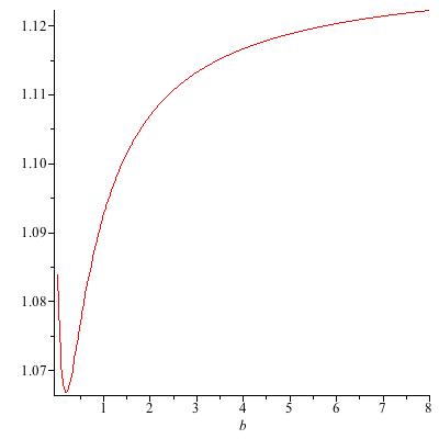
Refer to caption

Figure 5: For domains with area π\pi, the ratio λ1​(square)/λ1​(circle)\lambda_{1}({\rm square})/\lambda_{1}({\rm circle}) plotted against β\beta. For domains both with the same area, but different from π\pi, the curves are different but remain greater than 1

Various checks of the results shown in Figure 5 are possible. When β=0\beta=0, λ1​(circle)=j02≈5,783\lambda_{1}({\rm circle})=j_{0}^{2}\approx 5,783 with j0j_{0} the smallest zero of J0J_{0}, and λ1​(square)=2​π\lambda_{1}({\rm square})=2\pi, so the ratio is approximately 1.086.

We also compare λ1\lambda_{1} for rectangles of the same area with each other. See §A.1.2, in particular, Figure 8. In this connection, further development from equation (3.12) is given in Theorem 3 in §B.

3.5 Inequalities for λ1​□\lambda_{1\square} for a square, side 2​h2h

The formula for μ□2\mu_{\square}^{2} can be rewritten

1β=λ1​□2​tan⁡(|Ω|2​λ1​□2).\frac{1}{\beta}=\sqrt{\frac{\lambda_{1\square}}{2}}\tan\left(\frac{\sqrt{|\Omega|}}{2}\frac{\lambda_{1\square}}{2}\right). (3.16)

(Compare this with equation (3.5).)

Several items are immediate consequences of items in the previous subsection. Equation (3.10) gives

λ□=2​μ2∼2h​β=|∂Ω|β​|Ω|asβ→∞.\lambda_{\square}=2\mu^{2}\sim\frac{2}{h\beta}=\frac{|\partial\Omega|}{\beta|\Omega|}\qquad{\rm as\ }\ \beta\rightarrow\infty.

The following inequalities on tan⁡(x)\tan(x)

8​xπ2−4​x2<tan⁡(x)<x​π2π2−4​x2\frac{8x}{\pi^{2}-4x^{2}}<\tan(x)<\frac{x\pi^{2}}{\pi^{2}-4x^{2}} (3.17)

are established in [86].

Upper bounds on the tan function lead to lower bounds on μ⁡(r)\mu(r) while lower bounds on the tan function lead to upper bounds on μ⁡(r)\mu(r). Inequalities (3.17) lead to

μLB​(c,β)=πc⁡(4​c+π2​β)<μ⁡(c,β)<μUB​(c,β)=π4​β​(−1+1+4​βc).\mu_{\rm LB}(c,\beta)={\frac{\pi}{\sqrt{c\left(4\,c+{\pi}^{2}\beta\right)}}}<\mu(c,\beta)<\mu_{\rm UB}(c,\beta)=\frac{\pi}{4\beta}\,\left(-1+\sqrt{1+4\,{\frac{\beta}{c}}}\right). (3.18)

In particular, the formula for μLB​(h,β)\mu_{\rm LB}(h,\beta) gives

λ□>2β​h+4​h2/π2.\lambda_{\square}>\frac{2}{\beta h+4h^{2}/\pi^{2}}.

Other bounds can be established. For example, for all r>0r>0,

λ□>2h​β−2β2−4​r​(r2+1)β​h​(r4+1),soλ□>2h​β−2β2.\lambda_{\square}>\frac{2}{h\beta}-\frac{2}{\beta^{2}}-\frac{4r(r^{2}+1)}{\beta h(r^{4}+1)},\qquad{\rm so\ }\ \lambda_{\square}>\frac{2}{h\beta}-\frac{2}{\beta^{2}}.

This follows from equation (B.7) on using that 𝒱x>0{\cal V}_{x}>0 and 𝒱y>0{\cal V}_{y}>0.

3.6 The modulus of asymmetry for the equilateral triangle and for rectangles

See [28] for some calculations of the modulus of asymmetry (see §9.1) for various domains. The interest here is in how it might relate to quantitative estimates of the difference between the functionals for Ω\Omega and for the disk of the same area Ω∗\Omega^{*}.

4 Steady flows

4.1 The main theorem

There have been many studies of these, sometimes oriented towards exact solutions, sometimes numerical approximations, and sometimes checking theory against experiment: see e.g. [3, 77, 82, 83] and [81].

For given Ω\Omega and Δ​p>0\Delta{p}>0 there is a unique solution for uu and it is positive in Ω\Omega (Theorem 2.3 of  [47], but well known before this). The solutions at different β\beta vary monotonically with β\beta (as shown in Theorem 2.4 of  [47]). The effects of varying the domains Ω\Omega are more difficult to study: there is monotonicity with domain inclusion when β=0\beta=0 (Theorem 2.6 of  [47]) but not generally when β≠0\beta\neq{0}.

We now reference the proof of the first sentence in the Abstract. The area of Ω\Omega is denoted by |Ω||\Omega|. When β=0\beta=0 the result is called the St Venant inequality. The proof techniques for non-zero β\beta differ from the ‘symmetrisation’ proof techniques used for the earlier proofs for β=0\beta=0. The pure mathematical papers write that they denote by Ω∗\Omega^{*} the ‘ball’ with the same ‘volume’ as Ω\Omega: in our 2-dimensional case, Ω∗\Omega^{*} is the (circular) disk of radius |Ω|/π\sqrt{|\Omega|/\pi}.

Theorem 1.

For every β>0\beta>0, for every bounded Lipschitz set Ω⊂RN\Omega\subset{R^{N}}, the following inequality holds

Qsteady​(Ω,β)≤Qsteady​(Ω∗,β).Q_{{\rm steady}}(\Omega,\beta)\leq Q_{\rm steady}({\Omega^{*}},\beta). (4.1)

This is Theorem 1.1 of [16]. (Caution. The β\beta of [16] is the reciprocal of our β\beta.) The expression on the right hand side of equation (4.1) is given by equation (2.4) with a=|Ω|/πa=\sqrt{|\Omega|/\pi}.

Formulae for Qsteady​(β)Q_{\rm steady}(\beta) for various shapes are given in [60]. Other inequalities, for general Ω\Omega, are given in [47]. Related work is presented in [8].

4.2 QsteadyQ_{\rm steady}: circle compared with equilateral triangle and square

The formula for Qsteady​(circle)Q_{\rm steady}({\rm circle}) is given in equation (2.4). Figures 2 (for the triangle) and 4 (for the square) provide examples consistent with Theorem 1.

5 Transient Flows

5.1 An isoperimetric result

The second sentence of the Abstract follows from the representation (1.11), noting that λ1\lambda_{1} is the least of the eigenvalues, and the following theorem.

Theorem 2.

For every β>0\beta>0, for every bounded open Lipschitz set Ω⊂RN\Omega\subset{R^{N}}

λ1​(Ω,β)≥λ1​(Ω∗,β).\lambda_{1}(\Omega,\beta)\geq\lambda_{1}({\Omega^{*}},\beta). (5.1)

with equality if and only if Ω=Ω∗\Omega=\Omega^{*}.

This is the N=2N=2, q=2q=2 case of Theorem 2.1 of [16]. (The paper [16] titles Theorem 2.1 as A family of Faber-Krahn inequalities.) The theorem was first proved, in the N=2N=2 case in [11] (see also [10, 12], and the general NN case in [21]. Related work is presented in [13, 14, 15, 20, 21]. The expression on the right hand side of equation (5.1) is given by equation (2.6) with a=|Ω|/πa=\sqrt{|\Omega|/\pi}.

5.2 λ1\lambda_{1}: circle compared with equilateral triangle and square

Figures 3(for the triangle) and 5 (for the square) provide examples consistent with Theorem 2.

6 Illustrative examples of, and notes on, time-dependent flows

6.1 β=0\beta=0 and starting flows

The results of Theorems 1 and 2 have been known in the β=0\beta=0 case since 1949 and 1923 respectively. We suspect that graphical illustration of the kind shown in Figure 6 will be available in older literature, perhaps a century ago. The separation-of-variables, eigenfunction expansions are straightforward to find in several domain shapes, circles and rectangles being common examples. We have already cited [6] for the circle while the rectangle is treated, for example, in [27], though we expect the first publication of these might well be over a century ago. In Figure 6 we show plots of Q⁡(t)Q(t) for a circle of unit radius and a square with sides π\sqrt{\pi}.

Figure 6: The left hand plots are of Q⁡(t)Q(t): the right hand plots are of Q⁡(t)/Q⁡(∞)Q(t)/Q(\infty). The plots for the circular cross section are shown by the solid (red) curve: those for the square cross section are shown dotted (blue) with a small square symbol.

The left hand plots illustrate that the disk has the larger Q⁡(∞)Q(\infty). The right hand plots illustrate that the approach to Q⁡(∞)Q(\infty) is slower for the circular cross section than for others.

It is also easy to plot Q⁡(t,square)/Q⁡(t,circle)Q(t,{\rm square})/Q(t,{\rm circle}). The values in [71] can be used to check the behaviour at very large time as, for domains with area π\pi, Qsteady​(circle)=π/8≈0.3927Q_{\rm steady}({\rm circle})=\pi/8\approx{0.3927} and Qsteady​(square)≈0.3469Q_{\rm steady}({\rm square})\approx{0.3469}.

6.2 β>0\beta>0: comparing λ1\lambda_{1}

The results are less striking for large β\beta. In particular, when β\beta is very large the situation is essentially like that when unu_{n} is an appropriate constant around the boundary, uu is constant across Ω\Omega and Q⁡(t)Q(t) is approximately t​|Ω|​Δ​pt|\Omega|\Delta{p}, and there is no dependence on the shape of Ω\Omega (at the lowest order in the approximation for β\beta large).

6.3 A few more results valid for β>0\beta>0

6.3.1 Other checks on ϕn\phi_{n}

See [71] p107:

|Ω|=∑n=1∞(∫Ωϕn)2∫Ωϕn2.|\Omega|=\sum_{n=1}^{\infty}\frac{\left(\int_{\Omega}\phi_{n}\right)^{2}}{\int_{\Omega}\phi_{n}^{2}}.

Similarly the polar moment of inertia about the centroid satisfies

Ic=∑n=1∞∫Ω|z−zc|2​ϕn​(z)​∫Ωϕn∫Ωϕn2.I_{c}=\sum_{n=1}^{\infty}\frac{\int_{\Omega}|z-z_{c}|^{2}\phi_{n}(z)\int_{\Omega}\phi_{n}}{\int_{\Omega}\phi_{n}^{2}}.

6.3.2 QsteadyQ_{\rm steady}

𝐂𝐨𝐧𝐣𝐞𝐜𝐭𝐮𝐫𝐞Qsteady​(Ω∗,β)−Qsteady​(Ω,β)Qsteady​(Ω∗,β)→0asβ→∞.

6.3.3 The decay rate λ1\lambda_{1} when β>0\beta>0

Some monotonicity results for the principal eigenvalue of the generalized Robin problem are established in [35]. Their α=−1/β\alpha=-1/\beta; their λ\lambda has the opposite sign to ours, and it is our sign we use in this report. Before treating monotonicity aspects we repeat items they report: The eigenvalue λ1​(β)\lambda_{1}(\beta) is simple, and that an eigenfunction ϕ1(.,β)\phi_{1}(.,\beta) can be chosen with a single sign and normalized by letting the integral of its square over Ω\Omega being 1. In addition, as β→0\beta\rightarrow{0}, λ1​(β)\lambda_{1}(\beta) converges to the principal eigenvalue for the Dirichlet problem. Also

limβ→∞λ1​(β)​β=|∂Ω||Ω|.\lim_{\beta\rightarrow\infty}{\lambda_{1}(\beta)}{\beta}=\frac{|\partial\Omega|}{|\Omega|}.

There are partial monotonicity results.

  • •

    Let B⊂RnB\subset{R^{n}} n≥2n\geq{2} be a ball and Ω⊂B\Omega\subset{B}. If α<0\alpha<0 then λ1​(Ω1,α)>λ1​(B,α)>0\lambda_{1}(\Omega_{1},\alpha)>\lambda_{1}(B,\alpha)>0.

  • •

    Again, let α<0\alpha<0. If Ω⊂Rn\Omega\subset{R^{n}}, n≥2n\geq{2}, is a convex domain that contains a ball BB, then

    λ1​(B,α)≥λ1​(Ω,α)>0.\lambda_{1}(B,\alpha){\geq}\lambda_{1}(\Omega,\alpha)>0.

    (See Theorem 2 and Corollary 3 of  [35].)

  • •

    Let α<0\alpha<0 and Ω1⊂B⊂Ω2\Omega_{1}\subset{B}\subset{\Omega_{2}} where B⊂RnB\subset{R^{n}} n≥2n\geq{2} is a ball and Ω1\Omega_{1}, Ω2\Omega_{2} are convex domains, we have that λ1​(Ω1,α)≥λ1​(Ω2,α)>0\lambda_{1}(\Omega_{1},\alpha){\geq}\lambda_{1}(\Omega_{2},\alpha)>0

6.4 Further results applicable when β=0\beta=0

6.4.1 Isoperimetric results for some geometric functionals

Strictly speaking this subsubsection doesn’t require β=0\beta=0. However, at present our applications of the geometric functionals in connection with QsteadyQ_{\rm steady} and λ1\lambda_{1} are just for the case β=0\beta=0.

In this version of these notes, the other geometric domain functionals we consider are, the perimeter |∂Ω||\partial\Omega|, the polar moment of inertia IcI_{c} and BB defined – for star-shaped domains – by equation (6.1).

B⁡(z0)=∫∂Ωd​sn⋅(z−z0)andB=minz0∈Ω⁡B⁡(z0).B(z_{0})=\int_{\partial\Omega}\frac{ds}{n\cdot(z-z_{0})}\qquad{\rm and\ }\qquad B=\min_{z_{0}\in\Omega}B(z_{0}). (6.1)

For domains in the plane, see [71] for Polya’s proof that

2​Icπ≤(|∂Ω|2​π)4\frac{2I_{c}}{\pi}\leq\bigl(\frac{|\partial\Omega|}{2\pi}\bigr)^{4} (6.2)

Equality is attained only for disks. (Hadwiger gave a different proof, one which generalizes to RnR^{n}. For references, see [46].) We remark that a combination of this (6.2) and another easier-to-prove inequality, represents a refinement of the classical (|Ω|,|∂Ω|)(|\Omega|,|\partial\Omega|), area-perimeter, isoperimetric inequality:

(|Ω|π)2≤2​Icπ≤(|∂Ω|2​π)4.\bigl(\frac{|\Omega|}{\pi}\bigr)^{2}\leq\frac{2I_{c}}{\pi}\leq\bigl(\frac{|\partial\Omega|}{2\pi}\bigr)^{4}. (6.3)

We first note that connectedness is essential for inequality (6.2). For, if we let the domain be the union of two equal disjoint disks, symmetically placed either side of the origin so that the centroid is at the origin, we have a counterexample. By taking the components further apart we can increase IcI_{c} indefinitely, while |∂Ω||\partial\Omega| stays fixed. However, on joining the disks by a straight line the perimeter increases and this dumbell shaped domain does satisfy inequality (6.2).

Polya’s proof begins with conformal mapping, and requires the domain to be simply connected. Inequality (6.2) can be shown to be true for multiply-connected ones too: see [46].

6.4.2 Physical functionals: isoperimetric results applicable when β=0\beta=0

It was conjectured by Polya and Szego that among sets with given torsional rigidity QsteadyQ_{\rm steady}, balls minimize λ1\lambda_{1}. specifically

Qsteady​λ12≥π8​j4.Q_{\rm steady}\lambda_{1}^{2}\geq\frac{\pi}{8}j^{4}. (6.4)

This is proved in [50, 51].

The Payne-Rayner inequality, proved in [69], s relevant to estimating Q1​(β=0)Q_{1}(\beta=0). It states

Q1≥4​πλ12.Q_{1}\geq\frac{4\pi}{\lambda_{1}^{2}}.

Furthermore, there is equality when Ω\Omega is a disk. We remark that for the unit disk

Qn​(disk)=4​πjn4,Q_{n}(\rm disk)=\frac{4\pi}{j_{n}^{4}},

where jnj_{n} is the nn-th positive zero of J0J_{0}.

There are many more isoperimetric inequalities. With BB defined – for star-shaped domains – by equation (6.1), [71] p93 and p94 give

Qsteady≥|Ω|24​B,λ1≤j2​B2​|Ω|.Q_{\rm steady}\geq\frac{|\Omega|^{2}}{4B},\qquad\lambda_{1}\leq\frac{j^{2}B}{2|\Omega|}.

The first of these is an equality when Ω\Omega is an ellipse: see [71] p262. Other inequalities involving BB include

λ1≤j2​B2​|Ω|,\lambda_{1}\leq j^{2}\frac{B}{2|\Omega|},

(see [71]) which gives an equality when Ω\Omega is a disk. The functional BB occurs in an inequality involving Q1Q_{1},

Q1≤4​Bλ12.Q_{1}\leq\frac{4B}{\lambda_{1}^{2}}.

See [19, 44].

6.4.3 Some other results when β=0\beta=0 and Ω\Omega is convex

When Ω\Omega is convex,

  • •

    the steady solution, torsion function, has a square root which is concave;

  • •

    the principal eigenfunction ϕ1>0\phi_{1}>0 is such that log⁡(ϕ1)\log(\phi_{1}) is concave.

Let Ω0\Omega_{0} and Ω1\Omega_{1} be convex, and define the Minkowski sum

Ωt=(1−t)​Ω0+t​Ω1.\Omega_{t}=(1-t)\Omega_{0}+t\Omega_{1}.
  • •

    Qsteady​(0,Ωt)1/4Q_{\rm steady}(0,\Omega_{t})^{1/4} is concave. See [9].

  • •

    λ1(0,Ωt)−1/2\lambda_{1}(0,\Omega_{t})^{-1/2} is concave.

7 Symmetrisation

Theorem [71] Symmetrization of a plane domain with respect to a line leaves the area unchanged, but decreases the perimeter, polar moment of inertia about the centroid.
See [71]p6. In connection with moments of inertia, Steiner symmetrization about the line through the centroid reduces the moment associated with the direction perpendicular to the line, and leaves unchanged that associated with the direction of the line.

See [71] for the use of symmetrisation in proving

  • •

    for β=0\beta=0, QsteadyQ_{\rm steady} increases,

  • •

    for β=0\beta=0, λ1\lambda_{1} decreases.

The methods are only applicable in the case β=0\beta=0. See also the Appendix to this paper.

8 Overview: Perturbations from circular domains

Theorems 1 and 2 say nothing about by how much the quantities for some cross-section differ from those of a circular channel of the same cross-sectional area. Furthermore for domains Ω\Omega with given area |Ω||\Omega|, Theorem 1 is an upper bound on Qsteady​(Ω)Q_{\rm steady}(\Omega), while Theorem 2 is an lower bound on λ1​(Ω)\lambda_{1}(\Omega). Also of interest are bounds on the other side with various forms of geometric restrictions. And there are many other improvements that are possible, and many more that have been conjectured but remain unproven. For example, when β=0\beta=0, [71]p112 report a result (of Nicolai) from the 1920s that

Qsteady≤Imax​IminImax+Imin,Q_{\rm steady}\leq\frac{I_{\rm max}I_{\rm min}}{I_{\rm max}+I_{\rm min}}, (8.1)

where ImaxI_{\rm max} and IminI_{\rm min} are the principal moments of inertia about the centroid of Ω\Omega. Inequality (8.1) is an equality for any ellipse. With Ic=Imax+IminI_{c}=I_{\rm max}+I_{\rm min} from this we readily see

Qsteady≤Imax​IminImax+Imin≤Ic4,Q_{\rm steady}\leq\frac{I_{\rm max}I_{\rm min}}{I_{\rm max}+I_{\rm min}}\leq\frac{I_{c}}{4},

with the latter inequality an equality only for disks.

This section, and the next two, are primarily intended as a literature survey of items which seem relevant to these topics. There is an historical component to this. Rayleigh supported his conjecture on what has become known as the Faber-Krahn inequality with Fourier series approximations appropriate to nearly circular domains: this is described in [71]. Such asymptotics are the topic of §10.1. Before this we treat, in §9, methods less dependent on the perturbations being small. In §9.1 we indicate an area-based measure of asymmetry, one of many used in improving isoperimetric inequalities. In §9.2 we review bounds in terms of the classical geometric isoperimetric deficit. After these we consider nearly circular domains, first for the case β=0\beta=0 in §10.2, then, in work that hasn’t previously been published, for ellipses with β>0\beta>0 in §10.3,

9 Measuring the effect of departures from circular

9.1 A measure of asymmetry

Several decades ago Fraenkel defined a modulus of asymmetry

α⁡(Ω)=minz∈Ω​|Ω∖Ω∗​(z)||Ω|,\alpha(\Omega)={\rm min}_{z\in\Omega}\frac{|\Omega\setminus\Omega^{*}(z)|}{|\Omega|},

where Ω∗​(z)\Omega^{*}(z) is the disk centred at zz with the same area as Ω\Omega. See [30, 28]. Of course 0≤α⁡(Ω)≤10\leq\alpha(\Omega)\leq{1}. Since Ω\Omega and Ω∗​(z)\Omega^{*}(z) have the same area

|Ω∖Ω∗​(z)|=|Ω∗​(z)∖Ω|.|\Omega\setminus\Omega^{*}(z)|=|\Omega^{*}(z)\setminus\Omega|.

Note that some authors, perhaps most, use a symmetric difference, and hence have a modulus which is twice that of the definition above.

α⁡(Ω)\alpha(\Omega) for ellipses (x/a)2+(y​a)2=1(x/a)^{2}+(ya)^{2}=1, a≥1a\geq{1}.

The asymmetry α⁡(Ω)\alpha(\Omega) for an ellipse has been calculated several times, e.g. [28] but this might be susceptible to improvement, absolute values used as needed, as I would expect α⁡(ellipse⁡(a))=α⁡(ellipse⁡(1/a))\alpha({\rm ellipse}(a))=\alpha({\rm ellipse}(1/a)), and we would expect an even function of aa:

α⁡(ellipse)\displaystyle\alpha({\rm ellipse}) =2π​(arcsin​(a1+a2)−arcsin​(11+a2)),\displaystyle=\frac{2}{\pi}\left({\rm arcsin}\left(\frac{a}{\sqrt{1+a^{2}}}\right)-{\rm arcsin}\left(\frac{1}{\sqrt{1+a^{2}}}\right)\ \right),
=2π​(arctan⁡(a)−arctan⁡(1a))=2π​arctan​(a−1/a2),\displaystyle=\frac{2}{\pi}\left({\rm arctan}(a)-{\rm arctan}(\frac{1}{a})\ \right)=\frac{2}{\pi}{\rm arctan}\left(\frac{a-1/a}{2}\right),
∼1π​(2​(a−1)−(a−1)2+13​(a−1)3+…)as​a→1.\displaystyle\sim\frac{1}{\pi}\left(2(a-1)-(a-1)^{2}+\frac{1}{3}(a-1)^{3}+\dots\ \right)\qquad{\rm as\ }a\rightarrow{1}.

These expressions can be written in terms of ϵ\epsilon:

ϵ=a2−a−2a2+a−2∼2​(a−1)asa→1,\epsilon=\frac{a^{2}-a^{-2}}{a^{2}+a^{-2}}\sim 2(a-1)\qquad{\rm\ as\ }\ a\rightarrow{1},

As

(a−1a)2=a2+a−2−2=21−ϵ2−2,\left(a-\frac{1}{a}\right)^{2}=a^{2}+a^{-2}-2=\frac{2}{\sqrt{1-\epsilon^{2}}}-2,

we have

α⁡(ellipse)=2π​arctan​(12​(11−ϵ2−1)).\alpha({\rm ellipse})=\frac{2}{\pi}{\rm arctan}\left(\sqrt{\frac{1}{2}\left(\frac{1}{\sqrt{1-\epsilon^{2}}}-1\right)}\right).

The ellipse is also treated in [37], p89.

9.1.1 Improving the isoperimetric inequality for IcI_{c} in terms of α\alpha

This subsubsection is here in spite of the fact that, with the inequalities on QsteadyQ_{\rm steady} and λ1\lambda_{1} presented in this note to date, very few have any connection with IcI_{c}. However, the section is included as it illustrates, perhaps with the easiest domain functional for the purpose, that improvements to isoperimetric inequalities are possible.

One domain functional for which the isoperimetric inequality can be easily improved using this modulus of asymmetry is IcI_{c}, the polar moment of inertia about the centroid. The isoperimetric inequality is

Ic​(Ω∗)=|Ω|22​π≤Ic​(Ω).I_{c}(\Omega^{*})=\frac{|\Omega|^{2}}{2\pi}\leq I_{c}(\Omega)\ .

In 1986 (see [37], p87) the first author proved

Ic​(Ω∗)​(1+2​α​(Ω)2)≤Ic​(Ω),I_{c}(\Omega^{*})\left(1+2\alpha(\Omega)^{2}\right)\leq I_{c}(\Omega), (9.1)

which we have now seen, with a different proof, at page 198 of [38].

Consider polar moments about any point zz of Ω\Omega, and denote the disk centred zz with the same area as Ω\Omega by Ωz∗\Omega^{*}_{z}. Now, with the integrals being w.r.t area in the z′z^{\prime} variables (i.e. d​x′​d​y′dx^{\prime}dy^{\prime})

Iz(Ω)=∫Ω|z−z′|2,Ic(Ω)=minz∈ΩIz(Ω)and∫Ωz∗|z−z′|2=|Ω|22​π.I_{z}(\Omega)=\int_{\Omega}|z-z^{\prime}|^{2},\qquad I_{c}(\Omega)={\rm min}_{z\in\Omega}\ I_{z}(\Omega)\qquad{\rm and}\ \ \int_{\Omega^{*}_{z}}|z-z^{\prime}|^{2}=\frac{|\Omega|^{2}}{2\pi}.

Here IcI_{c} denotes the moment about the centroid, zcz_{c}, and the Parallel-Axes Theorem (one of several ingredients in the proof in  [38]) states:

Iz​(Ω)=Ic​(Ω)+|z−zc|2​|Ω|.I_{z}(\Omega)=I_{c}(\Omega)+|z-z_{c}|^{2}\,|\Omega|.

Our proof of inequality (9.1) is as follows. Since |Ω|=|Ωz∗||\Omega|=|\Omega_{z}^{*}|,

|Ω∖Ω|=|Ωz∗∖Ω|.|\Omega\setminus\Omega|=|{\Omega_{z}^{*}}\setminus\Omega|. (9.2)

We have

∫Ω|z−z′|2+∫Ωz∗|z−z′|2=∫Ω∪Ωz∗|z−z′|2+∫Ω∩Ωz∗|z−z′|2.\int_{\Omega}|z-z^{\prime}|^{2}+\int_{\Omega^{*}_{z}}|z-z^{\prime}|^{2}=\int_{\Omega\cup{\Omega^{*}_{z}}}|z-z^{\prime}|^{2}+\int_{\Omega\cap{\Omega^{*}_{z}}}|z-z^{\prime}|^{2}.

This is

Iz​(Ω)+|Ω|22​π=∫Ω∪Ωz∗|z−z′|2+∫Ω∩Ωz∗|z−z′|2.I_{z}(\Omega)+\frac{|\Omega|^{2}}{2\pi}=\int_{\Omega\cup{\Omega^{*}_{z}}}|z-z^{\prime}|^{2}+\int_{\Omega\cap{\Omega^{*}_{z}}}|z-z^{\prime}|^{2}.

Both the tems on the right can be bounded using the isoperimetric inequality, so

Iz​(Ω)+|Ω|22​π\displaystyle I_{z}(\Omega)+\frac{|\Omega|^{2}}{2\pi} ≥|Ω∪Ωz∗|2+|Ω∩Ωz∗|22​π\displaystyle\geq\frac{|{\Omega\cup{\Omega^{*}_{z}}}|^{2}+|{\Omega\cap{\Omega^{*}_{z}}}|^{2}}{2\pi}
=(|Ω|+|Ωz∗∖Ω|)2+(|Ω|−|Ω∖Ωz∗|)22​π\displaystyle=\frac{(|\Omega|+|{\Omega^{*}_{z}}\setminus\Omega|)^{2}+(|\Omega|-|\Omega\setminus{\Omega^{*}_{z}}|)^{2}}{2\pi}
=2​|Ω|2+2​|Ω∖Ωz∗|22​π.\displaystyle=\frac{2|\Omega|^{2}+2|\Omega\setminus{\Omega^{*}_{z}}|^{2}}{2\pi}.

In the last line we have used equation (9.2). We are free to choose zz, so take z=zcz=z_{c}, the centroid. Rearranging the last inequality gives

Ic​(Ω)≥|Ω|22​π​(1+2​|Ω∖Ωzc∗|2|Ω|2)≥|Ω|22​π​(1+2​α​(Ω)2),I_{c}(\Omega)\geq\frac{|\Omega|^{2}}{2\pi}\left(1+2\frac{|\Omega\setminus{\Omega^{*}_{z_{c}}}|^{2}}{|\Omega|^{2}}\right)\geq\frac{|\Omega|^{2}}{2\pi}\left(1+2\alpha(\Omega)^{2}\right),

as α⁡(Ω)\alpha(\Omega) is found from minimizing over the centres zz of the disks. This establishes the inequality (9.1). It is perhaps remarkable that repeated uses of the isoperimetric inequality yield an improvement on it. However there are many properties of the polar moment of inertia that enter the proof. First it is an additive domain functional, though only superadditivity is used. The first properties are

D⁡(Ω)+D⁡(Ω∗)≥D⁡(Ω∪Ω∗)+D⁡(Ω∩Ω∗)andD⁡(Ω)≥D⁡(Ω∗)​∀Ω,D(\Omega)+D(\Omega^{*})\geq D(\Omega\cup\Omega^{*})+D(\Omega\cap\Omega^{*})\qquad{\rm and}\qquad D(\Omega)\geq D(\Omega^{*})\ \forall\Omega\ ,

and the final property is the specific form of I⁡(Ω∗)I(\Omega^{*}) in terms of area. (Some slight generalization might be possible, e.g. for higher-order moments

Ip​(Ω,z)=∫Ω|z−z′|p,Ip​(Ω∗)=2​πp+2​(|Ω|π)(p+2)/2,I_{p}(\Omega,z)=\int_{\Omega}|z-z^{\prime}|^{p},\qquad I_{p}(\Omega^{*})=\frac{2\pi}{p+2}\left(\frac{|\Omega|}{\pi}\right)^{(p+2)/2},

satisfies the properties mentioned in general for domain functional DD but a more elaborate relation involving |Ω∖Ω∗||\Omega\setminus\Omega^{*}| arises at the end of the calculation.)

We record the items below as other inequalities can be found. Cauchy-Schwarz gives the rightmost of

(|Ω|−|Ω∖Ωz∗|)22​π=|Ω∩Ωz∗|22​π≤∫Ω∩Ωz∗|z−z′|2=∫|z−z′|​χΩ​|z−z′|​χΩz∗≤Iz​(Ω)​|Ω|22​π,\frac{(|\Omega|-|\Omega\setminus{\Omega^{*}_{z}}|)^{2}}{2\pi}=\frac{|\Omega\cap{\Omega^{*}_{z}}|^{2}}{2\pi}\leq\int_{\Omega\cap{\Omega^{*}_{z}}}|z-z^{\prime}|^{2}=\int|z-z^{\prime}|\chi_{\Omega}\ |z-z^{\prime}|\chi_{\Omega^{*}_{z}}\leq\sqrt{I_{z}(\Omega)\frac{|\Omega|^{2}}{2\pi}},

where the characteristic functions χ\chi have arguments z′z^{\prime}. Making use of the fact that the square of the radius of Ωz∗{\Omega^{*}_{z}} is |Ω|/π|\Omega|/\pi,

α​(Ω)2​|Ω|22​π≤|Ωz∗∖Ω|22​π\displaystyle\alpha(\Omega)^{2}\frac{|\Omega|^{2}}{2\pi}\leq\frac{|{\Omega^{*}_{z}\setminus{\Omega}}|^{2}}{2\pi} ≤∫Ωz∗∖Ω|z−z′|2≤|Ωz∗∖Ω|​|Ω|π,\displaystyle\leq\int_{\Omega^{*}_{z}\setminus{\Omega}}|z-z^{\prime}|^{2}\leq\frac{|{\Omega^{*}_{z}\setminus{\Omega}}||\Omega|}{\pi},
2​α​(Ω)​|Ω|22​π≤|Ω∖Ωz∗|​|Ω|π\displaystyle 2\alpha(\Omega)\frac{|\Omega|^{2}}{2\pi}\leq\frac{|\Omega\setminus{\Omega^{*}_{z}}||\Omega|}{\pi} ≤∫Ω∖Ωz∗|z−z′|2\displaystyle\leq\int_{\Omega\setminus{\Omega^{*}_{z}}}|z-z^{\prime}|^{2}

An aside. Let r¯​(Ω)\overline{r}(\Omega) denote the transfinute diameter (also known as logarithmic capacity or outer mapping radius). It is possible to use this, in tandem with the inequality

Ic≤π2​r¯4equivalently(r⁡(Ω)¯r⁡(Ω∗)¯)4≥Ic​(Ω)Ic​(Ω∗).I_{c}\leq\frac{\pi}{2}{\overline{r}}^{4}\qquad{\rm equivalently}\ \ \left(\frac{\overline{r(\Omega)}}{\overline{r(\Omega^{*})}}\right)^{4}\geq\frac{I_{c}(\Omega)}{I_{c}(\Omega^{*})}.

See [71] p126. (Note the different uses of the overline here to later subsections, e.g. the table.)
Rewriting an earler inequality relating IcI_{c} to the perimeter |∂Ω||\partial\Omega|,

Ic≤π2​(|∂Ω|2​π)4equivalently(|∂Ω|4​π​|Ω|)4≥Ic​(Ω)Ic​(Ω∗).I_{c}\leq\frac{\pi}{2}\,\left(\frac{|\partial\Omega|}{2\pi}\right)^{4}\qquad{\rm equivalently}\ \ \left(\frac{|\partial\Omega|}{\sqrt{4\pi|\Omega|}}\right)^{4}\geq\frac{I_{c}(\Omega)}{I_{c}(\Omega^{*})}.

Hence the classical geometric inequality, concerning the isoperimetric deficit, is improved to

|∂Ω|24​π​|Ω|−1≥1+2​α​(Ω)2−1.\frac{|\partial\Omega|^{2}}{4\pi|\Omega|}-1\geq\sqrt{1+2\alpha(\Omega)^{2}}-1. (9.3)

Regular polygons. (Amongst the domains considered in detail in this paper are equilateral triangles and squares. See also §A.2.) The polar moment of inertia about the centre of a regular nn-gon is

Ic​(n−gon)=|Ω|26​n​(tan⁡(πn)+3​cot⁡(πn)).I_{c}(n{\rm-gon})=\frac{|\Omega|^{2}}{6n}\left(\tan(\frac{\pi}{n})+3\cot(\frac{\pi}{n})\right).

In the literature, e.g. [71] (where n=3n=3, 44 and 66 is given on pages 252, 256 and 258), the functionals are given in terms of side length, there denoted by aa. Then

|Ω|=n​a24​tan⁡(πn).|\Omega|=\frac{na^{2}}{4\tan(\frac{\pi}{n})}.

The isoperimetric deficit satisfies

|∂Ω|2−4​π​|Ω|=a2​n2​(1−π/ntan⁡(π/n))=4​|Ω|​π​tan⁡(π/n)π/n​(1−π/ntan⁡(π/n))∼4​|Ω|​π3​(πn)2,{|\partial\Omega|^{2}}-{4\pi|\Omega|}=a^{2}n^{2}\left(1-\frac{\pi/n}{\tan(\pi/n)}\right)=4|\Omega|\pi\frac{\tan(\pi/n)}{\pi/n}\left(1-\frac{\pi/n}{\tan(\pi/n)}\right)\sim\frac{4|\Omega|\pi}{3}\left(\frac{\pi}{n}\right)^{2},

as nn tends to infinity. The circumradius RR is related to the area by

|Ω|=n​R22​sin⁡(2​πn).|\Omega|=\frac{nR^{2}}{2}\sin(\frac{2\pi}{n}).

The inradius ρ\rho satisfies (by a simple application of Pythagoras’ Theorem)

R2−ρ2=a24,R^{2}-\rho^{2}=\frac{a^{2}}{4},

and hence is given by

ρ=R2−|Ω|​tan⁡(π/n)n.\rho=\sqrt{R^{2}-\frac{|\Omega|\tan(\pi/n)}{n}}.

The modulus of asymmetry has been calculated for various polygons in [28]. As an example

2​α​(square)=4π​(2​arccos⁡(π2)−12​π⁡(4−π))≈0.1810919377.2\alpha({\rm square})=\frac{4}{\pi}\left(2\arccos(\frac{\sqrt{\pi}}{2})-\frac{1}{2}\sqrt{\pi(4-\pi)}\right)\approx 0.1810919377\ .

Below we use the values of α⁡(Ω)\alpha(\Omega) from [28] to compare the left-hand and right-hand sides of the inequality (9.3).

nn 2​α​(Ω)2\alpha(\Omega) |∂Ω|24​π​|Ω|−1\frac{|\partial\Omega|^{2}}{4\pi|\Omega|}-1 2​π​Ic​(Ω)|Ω|−1\frac{\sqrt{2\pi I_{c}(\Omega)}}{|\Omega|}-1 1+2​α​(Ω)2−1\sqrt{1+2\alpha(\Omega)^{2}}-1
3 0.3649426110 3​3π−1=0.653986686\frac{3\sqrt{3}}{\pi}-1=0.653986686 0.099636111 0.032759195
4 0.1810919377 4π−1=0.273239544\frac{4}{\pi}-1=0.273239544 0.023326708 0.008165237
6 0.0744657545 2​3π−1=0.102657791\frac{2\sqrt{3}}{\pi}-1=0.102657791 0.003825838 0.001385327
nn tan⁡(π/n)π/n−1\frac{\tan(\pi/n)}{\pi/n}-1 π3​n​(tan⁡(πn)+3​cot⁡(πn))−1\sqrt{\frac{\pi}{3n}\left(\tan(\frac{\pi}{n})+3\cot(\frac{\pi}{n})\right)}-1
n>>1n>>1 π23​n2\frac{\pi^{2}}{3n^{2}} 2​π445​n4\frac{2\pi^{4}}{45n^{4}}
∞\infty 0 0 0 0

9.1.2 Improving other isoperimetric inequalities in terms of α\alpha

When β=0\beta=0, the modulus of asymmetry α\alpha is used to bound the departure of λ1\lambda_{1} in [34]. In the inequality following their equation (2), for our situation of the ordinary Laplacian and the plane,

λ1​(Ω)≥λ1​(Ω∗)​(1+c​α​(Ω)4)\lambda_{1}(\Omega)\geq\lambda_{1}(\Omega^{*})\left(1+c\,\alpha(\Omega)^{4}\right)

for some constant c>0c>0. (When estimating cc, recall that our modulus of asymmetry differs by a factor of 22 from that in [34].)

The isoperimetric deficit is used to bound the departure of the eigenvalues in [67]. See also [58].

Regular polygons, and β=0\beta=0. Data on these is available in [71], e.g. for λ1\lambda_{1}:

  • •

    equilateral triangle λ1​|Ω|=4​π23=22.793\lambda_{1}|\Omega|=\frac{4\pi^{2}}{\sqrt{3}}=22.793

  • •

    square λ1​|Ω|=2​π2=19.7392\lambda_{1}|\Omega|=2\pi^{2}=19.7392

  • •

    regular hexagon

  • •
  • •

    circle λ1​|Ω|=π​j2=18.168\lambda_{1}|\Omega|=\pi\,j^{2}=18.168

9.2 β=0\beta=0 and bounds in terms of the classical isoperimetric deficit |∂Ω|2−4​π​|Ω||\partial\Omega|^{2}-4\pi|\Omega|

Defining Ψ=1−4​π​|Ω|/|∂Ω|2\Psi=1-4\pi|\Omega|/|\partial\Omega|^{2}, [68] inequality (4.12) gives

Qsteady​(Ω)≥|Ω|28​π​(1−2​Ψ2​(1−Ψ2)−1−4​Ψ4​(1−Ψ2)−2​log⁡(Ψ))when ​β=0.Q_{\rm steady}(\Omega)\geq\frac{|\Omega|^{2}}{8\pi}\left(1-2\Psi^{2}(1-\Psi^{2})^{-1}-4\Psi^{4}(1-\Psi^{2})^{-2}\log(\Psi)\right)\qquad\mbox{\rm when\ }\beta=0.

There are also results for λ1\lambda_{1}, and conjectures, e.g. the following.

Conjecture. (Taken from [31]:see their equation (12).) It is conjectured (in [1]) that for simply-connected plane domains

λ1​(Ω)≤π​j2|Ω|+π24​|∂Ω|2−4​π​|Ω||Ω|2.\lambda_{1}(\Omega)\leq\frac{\pi j^{2}}{|\Omega|}+\frac{\pi^{2}}{4}\,\frac{|\partial\Omega|^{2}-4\pi|\Omega|}{|\Omega|^{2}}.

Equality occurs not only for the disc but also asymptotically on infinite rectangular strips.

9.2.1 Relations between the classical isoperimetric deficit and α⁡(Ω)\alpha(\Omega)

See [33].

10 Nearly circular domains

10.1 Geometric preliminaries, nearly circular domains

The domain functionals QsteadyQ_{\rm steady} and λ1\lambda_{1} involve pde problems, and much effort has been expended seeking to bound these in terms of simpler geometric functionals. Thus Theorems 1 and 2 give inequalities involving the area, |Ω||\Omega|. Besides area, there are other geometric functionals, perimeter, polar moment of inertia about the centroid, etc.

In much of this section we treat boundaries whose equation in polar form is

r=a⁡(1+ρ⁡(θ))with​a=1.r=a(1+\rho(\theta))\qquad{\rm with\ }a=1.

For most of this we consider ρ\rho small. In connection with small perturbations for a circle, we follow the methods given in [71], p53. There the boundary of the domain is given by

r=1+δ​ρ¯​(θ)r=1+\delta{\overline{\rho}}(\theta)

with δ\delta a first-order small quantity. The boundary function is given as a Fourier series

ρ⁡(θ)=a0+∑n=1∞(an​cos⁡(n​θ)+bn​sin⁡(n​θ)).\rho(\theta)=a_{0}+\sum_{n=1}^{\infty}(a_{n}\cos(n\theta)+b_{n}\sin(n\theta)). (10.1)

(Caution. The Fourier coefficients with n≥1n\geq{1} in [71] equation (1) are half ours as they have a factor of 2 outside their sum.)

Various geometric functionals are considered in [71]: perimeter |∂Ω||\partial\Omega|, polar moment of inertia IcI_{c}, etc.. These can be approximated using ρ\rho small: We begin with considerations of the area.

10.1.1 Area |Ω||\Omega|

With the boundary described by equation (10.1) the area of Ω\Omega is given by

|Ω|π=(1+a0)2+12​∑n=1∞(an2+bn2).\frac{|\Omega|}{\pi}=(1+a_{0})^{2}+\frac{1}{2}\sum_{n=1}^{\infty}(a_{n}^{2}+b_{n}^{2}). (10.2)

Ellipse

A test case for the methods is the ellipse x2a2+a2​y2≤1\frac{x^{2}}{a^{2}}+a^{2}y^{2}\leq{1}. In polar coordinates relative to the centre the boundary curve is

r\displaystyle r =1cos⁡(θ)2a2+a2sin(θ)2=2a2+a−2−(a2−a−2)​cos⁡(2​θ)\displaystyle=\frac{1}{\sqrt{\frac{\cos(\theta)^{2}}{a^{2}}+a^{2}\sin(\theta)^{2}}}=\sqrt{\frac{2}{{a}^{2}+{a}^{-2}-\left({a}^{2}-{a}^{-2}\right){\cos(2\theta)}}}
=r(π4)(1−a2−a−2a2+a−2cos(2θ))−1/2wherer(π4)=2a2+a−2\displaystyle=r\left(\frac{\pi}{4}\right)\left(1-\frac{a^{2}-a^{-2}}{a^{2}+a^{-2}}\cos(2\theta)\right)^{-1/2}\ \ {\rm where}\ \ r\left(\frac{\pi}{4}\right)=\sqrt{\frac{2}{{a}^{2}+{a}^{-2}}} (10.3)
=1+tan2⁡(θ)a−2+a2​tan2⁡(θ)\displaystyle=\sqrt{\frac{1+\tan^{2}(\theta)}{a^{-2}+a^{2}\tan^{2}(\theta)}} (10.4)

Without any assumptions on aa, the coefficients in the Fourier series for r⁡(θ)r(\theta) involve elliptic integrals. Our interest is in aa near 1. However (a−1)(a-1) might not be the best perturbation parameter. We have also used, in computations,

ϵ=a2−a−2a2+a−2∼2​(a−1)asa→1,\epsilon=\frac{a^{2}-a^{-2}}{a^{2}+a^{-2}}\sim 2(a-1)\qquad{\rm\ as\ }\ a\rightarrow{1},

and others, e.g. [23], use the eccentricity

e=1−1a4∼2​(a−1)1/2asa→1.e=\sqrt{1-\frac{1}{a^{4}}}\sim 2(a-1)^{1/2}\qquad{\rm\ as\ }\ a\rightarrow{1}.

Including an aa dependence in r⁡(a,θ)r(a,\theta) we remark that r⁡(1/a,θ)=r⁡(a,θ+π/2)r(1/a,\theta)=r(a,\theta+\pi/2) and ϵ⁡(1/a)=−ϵ⁡(a)\epsilon(1/a)=-\epsilon(a). The binomial expansions

r⁡(0)r⁡(π/4)\displaystyle\frac{r(0)}{r(\pi/4)} =(1−ϵ)−1/2=1+∑k=1∞(2​k)!22​k​(k!)2ϵk,\displaystyle=(1-\epsilon)^{-1/2}=1+\sum_{k=1}^{\infty}\frac{(2k)!}{2^{2k}(k!)^{2}}\ \epsilon^{k},
r⁡(θ)r⁡(π/4)\displaystyle\frac{r(\theta)}{r(\pi/4)} =(1−ϵcos(2θ))−1/2=1+∑k=1∞(2​k)!22​k​(k!)2cos(2θ))kϵk,\displaystyle=(1-\epsilon\cos(2\theta))^{-1/2}=1+\sum_{k=1}^{\infty}\frac{(2k)!}{2^{2k}(k!)^{2}}\ \cos(2\theta))^{k}\epsilon^{k}, (10.5)

may be useful in finding higher terms in the perturbation expansions of some domain functionals. The symmetries of the ellipse explain the form of the expansion:

  • •

    It is symmetric about θ=0\theta=0, hence only cosine terms.

  • •

    It is symmetric about θ=π/2\theta=\pi/2 and hence only the even order cosine terms cos⁡(2​m​θ)\cos(2m\theta).

  • •

    When ϵ\epsilon is replaced by −ϵ-\epsilon and θ\theta by θ+π/2\theta+\pi/2 the expression is unchanged and hence the form of the polynomial coefficients in ϵ\epsilon forming the Fourier coefficients. For mm is odd, only odd powers of ϵ\epsilon appear: for mm is even, only even powers of ϵ\epsilon appear.

We will see these symmetries in connection with ϕ1\phi_{1} and usteadyu_{\rm steady}. Returning to the study of the boundary curve, we also need the expansion for r⁡(π/4)r(\pi/4):

a2=1+ϵ1−ϵ,2r⁡(π/4)=a2+a−2=21−ϵ2,r⁡(π4)=(1−ϵ2)1/4.a^{2}=\sqrt{\frac{1+\epsilon}{1-\epsilon}},\qquad\frac{2}{r(\pi/4)}=a^{2}+a^{-2}=\frac{2}{\sqrt{1-\epsilon^{2}}},\qquad r\left(\frac{\pi}{4}\right)=\left(1-\epsilon^{2}\right)^{1/4}.

The first few terms give

r⁡(θ)=1+12​cos⁡(2​θ)​ϵ+(316​cos⁡(4​θ)−116)​ϵ2+O⁡(ϵ3).r(\theta)=1+\frac{1}{2}\,\cos\left(2\,\theta\right)\epsilon+\left(\frac{3}{16}\,\cos\left(4\,\theta\right)-\frac{1}{16}\right){\epsilon}^{2}+O(\epsilon^{3}).

Alternatively we can consider asymptotics as a→1a\rightarrow{1}. Then ρ=rellipse−1\rho=r_{\rm ellipse}-1 satisfies

ρ⁡(θ)\displaystyle\rho(\theta) ∼(a−1)​cos⁡(2​θ)−(14+12​cos⁡(2​θ)−34​cos⁡(4​θ))​(a−1)2+O⁡((a−1)3)\displaystyle\sim(a-1)\cos(2\theta)-(\frac{1}{4}+\frac{1}{2}\cos(2\theta)-\frac{3}{4}\cos(4\theta))(a-1)^{2}+O((a-1)^{3})
=−14​(a−1)2+((a−1)−12​(a−1)2)​cos⁡(2​θ)+34​(a−1)2​cos⁡(4​θ)+O⁡((a−1)3).\displaystyle=-\frac{1}{4}(a-1)^{2}+\left((a-1)-\frac{1}{2}(a-1)^{2}\right)\cos(2\theta)+\frac{3}{4}(a-1)^{2}\cos(4\theta)+O((a-1)^{3}). (10.6)

in the notation of equation (10.1)

a0=−14​(a−1)2+o⁡((a−1)2),a2=(a−1)+o⁡((a−1)),a_{0}=-\frac{1}{4}(a-1)^{2}+o((a-1)^{2}),\qquad a_{2}=(a-1)+o((a-1)),

and all other Fourier coefficients are of sufficiently small order that they are not needed in subsequent calculations in this paper. Of course we already know that the area of our ellipse is π\pi. The Fourier coefficients given in equation (10.6) for the approximation to the ellipse’s boundary inserted into equation (10.2) is consistent with this:

areaEllipseπ\displaystyle\frac{\rm areaEllipse}{\pi} ∼(1−14​(a−1)2)2+12​(a−1)2+O⁡((a−1)3),\displaystyle\sim\left(1-\frac{1}{4}(a-1)^{2}\right)^{2}+\frac{1}{2}(a-1)^{2}+O((a-1)^{3}),
=1+O⁡((a−1)3).\displaystyle=1+O((a-1)^{3}).

For calculations extending the use of higher order terms in the Fourier series (10.6). one might need formulae like

x2​n=21−2​n​(12​(2​nn)+∑j=1n(2​nn−j)​T2​j​(x)),x^{2n}=2^{1-2n}\left(\frac{1}{2}\binom{2n}{n}+\sum_{j=1}^{n}\binom{2n}{n-j}T_{2j}(x)\right),

and we plan, for elliptical Ω\Omega to implement this but have yet to do so.

We now consider general curves close to circular with the a0a_{0}, ana_{n} and bnb_{n} all small, O⁡(δ)O(\delta) or smaller. Equation (10.2) is

|Ω|π=(1+a0)2​(1+∑n=1∞(an2+bn2)2​(1+a0)2),\frac{|\Omega|}{\pi}=(1+a_{0})^{2}\left(1+\frac{\sum_{n=1}^{\infty}(a_{n}^{2}+b_{n}^{2})}{2(1+a_{0})^{2}}\right),

and hence, with the …\dots indicating smaller order terms

|Ω|π\displaystyle\sqrt{\frac{|\Omega|}{\pi}} ∼(1+a0)​(1+∑n=1∞(an2+bn2)4​(1+a0)2+…),\displaystyle\sim(1+a_{0})\left(1+\frac{\sum_{n=1}^{\infty}(a_{n}^{2}+b_{n}^{2})}{4(1+a_{0})^{2}}+\dots\right),
∼(1+a0)+14​∑n=1∞(an2+bn2)+….\displaystyle\sim(1+a_{0})+\frac{1}{4}\sum_{n=1}^{\infty}(a_{n}^{2}+b_{n}^{2})+\dots\ . (10.7)

10.1.2 Perimeter |∂Ω||\partial\Omega|

The approximation for the perimeter when ρ\rho is small is as follows. (Note the Caution given earlier about the difference in notation of our Fourier coefficients and those in [71].)

|∂Ω|\displaystyle|\partial\Omega| =∫02​πr2+(d​rd​θ)2​𝑑θ=∫02​π1+2​ρ+ρ2+(d​ρd​θ)2​𝑑θ\displaystyle=\int_{0}^{2\pi}\sqrt{r^{2}+(\frac{dr}{d\theta})^{2}}\,d\theta=\int_{0}^{2\pi}\sqrt{1+2\rho+\rho^{2}+(\frac{d\rho}{d\theta})^{2}}\ d\theta
∼2​π​∫02​π(1+12​(2​ρ+ρ2+(d​ρd​θ)2)−18​(2​ρ)2)​𝑑θ\displaystyle\sim 2\pi\int_{0}^{2\pi}\left(1+\frac{1}{2}(2\rho+\rho^{2}+(\frac{d\rho}{d\theta})^{2})-\frac{1}{8}(2\rho)^{2}\right)\ d\theta
OPEN∼2​π​∫02​π(1+ρ+12​(d​ρd​θ)2))​𝑑θ\displaystyle\sim 2\pi\int_{0}^{2\pi}\left(1+\rho+\frac{1}{2}(\frac{d\rho}{d\theta})^{2})\right)\ d\theta
|∂Ω|2​π\displaystyle\frac{|\partial\Omega|}{2\pi} ∼1+a0+14​∑n=1∞n2​(an2+bn2).\displaystyle\sim 1+a_{0}+\frac{1}{4}\sum_{n=1}^{\infty}n^{2}\left(a_{n}^{2}+b_{n}^{2}\right). (10.8)

Ellipse

The perimeter of our ellipse, area π\pi, can be given without any approximation of small eccentricity ee, by

|∂Ω|=4aEllipticE(e)∼2πa(1−e24−3​e464…)fora→1.|\partial\Omega|=4a\,{\rm EllipticE}(e)\sim 2\pi a\left(1-\frac{e^{2}}{4}-\frac{3e^{4}}{64}\ \ldots\ \ \right)\ \qquad{\rm for\ }\ \ a\rightarrow 1.

Thus with e2∼2​ϵ−2​ϵ2e^{2}\sim{2\epsilon}-2\epsilon^{2} and a∼1+ϵ/2+ϵ2/8a\sim{1+\epsilon/2+{\epsilon^{2}}/8},

|∂Ω|∼2​π​(1+316​ϵ2+…)forϵ→0.|\partial\Omega|\sim 2\pi(1+\frac{3}{16}\epsilon^{2}+\ \ \ldots)\qquad{\rm for\ }\ \epsilon\rightarrow 0. (10.9)

10.1.3 Polar moment of inertia about the centroid IcI_{c}

The polar moment of inertia is, taking the origin at the centroid is

Ic=∫Ω((x−xc)2+(y−yc)2),I_{c}=\int_{\Omega}\left((x-x_{c})^{2}+(y-y_{c})^{2}\right),

where zc=(xc,yc)z_{c}=(x_{c},y_{c}) is the centroid of Ω\Omega. When the boundaries are given in polar coordinates, this is

Ic=14​∫02​πr​(θ)4​𝑑θ.I_{c}=\frac{1}{4}\int_{0}^{2\pi}r(\theta)^{4}\ d\theta.

Ellipse

For our disk and ellipse these are

Ic​(disk)=π2​a4,Ic​(ellipse)=π4​(a2+a−2)=π2​1−ϵ2.I_{c}({\rm disk})=\frac{\pi}{2}a^{4},\qquad I_{c}({\rm ellipse})=\frac{\pi}{4}(a^{2}+a^{-2})=\frac{\pi}{2\sqrt{1-\epsilon^{2}}}. (10.10)

The asymptotics below check with the entries in the table of  [71] reproduced in a later subsection:

2​Ic​(ellipse)π\displaystyle\frac{2I_{c}({\rm ellipse})}{\pi} ∼1+2​(a−1)2as​a→1,\displaystyle\sim 1+2(a-1)^{2}\qquad{\rm as\ }a\rightarrow 1,
(2​Ic​(ellipse)π)1/4\displaystyle\left(\frac{2I_{c}({\rm ellipse})}{\pi}\right)^{1/4} OPEN∼1+12​(a−1)2+o​(a−1)2)as​a→1,\displaystyle\sim 1+\frac{1}{2}(a-1)^{2}+o(a-1)^{2})\qquad{\rm as\ }a\rightarrow 1,
OPEN∼1+a0+34​a22+o​(a−1)2)as​a→1.\displaystyle\sim 1+a_{0}+\frac{3}{4}a_{2}^{2}+o(a-1)^{2})\qquad{\rm as\ }a\rightarrow 1.

10.2 Nearly circular domains with β=0\beta=0

First we treat the case β=0\beta=0 and seek approximations, notably for QsteadyQ_{\rm steady} and λ1\lambda_{1}. We follow [71] in expressing the asymptotics (at small δ\delta) as

Quantity=1+a0+14​∑n=1∞R⁡(n)​(an2+bn2).{\mbox{\rm Quantity}}=1+a_{0}+\frac{1}{4}\sum_{n=1}^{\infty}R(n)(a_{n}^{2}+b_{n}^{2}).

(The factor 14\frac{1}{4} is because of differing definitions of ana_{n} and bnb_{n}.) Use an overline, as in [71], p33 to denote various radii.

10.2.1 The eigenvalue λ1\lambda_{1} at β=0\beta=0

[71] report that Rayleigh found

jλ1=λ1¯=1+a0−14​∑n=1∞(1+2​j​Jn′​(j)Jn​(j))​(an2+bn2).\frac{j}{\sqrt{\lambda_{1}}}={\overline{\lambda_{1}}}=1+a_{0}-\frac{1}{4}\sum_{n=1}^{\infty}\left(1+\frac{2j{J_{n}}^{\prime}(j)}{J_{n}(j)}\right)(a_{n}^{2}+b_{n}^{2}).

Here the λ1¯\overline{\lambda_{1}} denotes the radius of the disk with principal eigenvalue λ1\lambda_{1}. Numeric values of the nn-th term, involving the Bessel functions, are readily computed. The n=1n=1 term is −1-1. The rest are positive. Furthermore as shown in [71] p133 equation (2)

2​n−3≤(1+2​j​Jn′​(j)Jn​(j))<2​n+1,2n-3\leq\left(1+\frac{2j{J_{n}}^{\prime}(j)}{J_{n}(j)}\right)<2n+1,

with equality (in the left hand expression) only when n=1n=1.
At large nn, we have (1+2​j​Jn′​(j)Jn​(j))∼2​n+1\left(1+\frac{2j{J_{n}}^{\prime}(j)}{J_{n}(j)}\right)\sim 2n+1. The expressions (1+2​j​Jn′​(j)Jn​(j))\left(1+\frac{2j{J_{n}}^{\prime}(j)}{J_{n}(j)}\right) can, at each nn, be written as a rational function of jj.

For an ellipse one finds

jλ1​(ellipse)\displaystyle\frac{j}{\sqrt{\lambda_{1}({\rm ellipse})}} ∼1−14​(a−1)2−14​(1+2​j​J2′​(j)J2​(j))​(a−1)2+o⁡((a−1)2)\displaystyle\sim 1-\frac{1}{4}(a-1)^{2}-\frac{1}{4}\left(1+\frac{2j{J_{2}}^{\prime}(j)}{J_{2}(j)}\right)(a-1)^{2}+o((a-1)^{2})
λ1​(ellipse)j2\displaystyle\frac{\lambda_{1}({\rm ellipse})}{j^{2}} ∼1+12​(a−1)2+12​(1+2​j​J2′​(j)J2​(j))​(a−1)2+o⁡((a−1)2)\displaystyle\sim 1+\frac{1}{2}(a-1)^{2}+\frac{1}{2}\left(1+\frac{2j{J_{2}}^{\prime}(j)}{J_{2}(j)}\right)(a-1)^{2}+o((a-1)^{2})
∼1+(1+j​J2′​(j)J2​(j))​(a−1)2+o⁡((a−1)2)\displaystyle\sim 1+\left(1+\frac{j{J_{2}}^{\prime}(j)}{J_{2}(j)}\right)(a-1)^{2}+o((a-1)^{2})
∼1+(j22−1)​(a−1)2+o⁡((a−1)2),\displaystyle\sim 1+\left(\frac{j^{2}}{2}-1\right)(a-1)^{2}+o((a-1)^{2}), (10.11)
∼1+1.891592982​(a−1)2+o⁡((a−1)2).\displaystyle\sim 1+1.891592982\ (a-1)^{2}+o((a-1)^{2}).

Without the special interest in nearly circular, eigenvalues for elliptical domains have been investigated before, with Mathieu functions in the eigenfunctions: see  [78, 23, 42]. In particular [23] equation (3.5) reports that [42] gave the approximation:

λa=j⁡(1−e4−c4​e4−c6​e6−c8​e8),\frac{\sqrt{\lambda}}{a}=j\left(1-\frac{e}{4}-c_{4}e^{4}-c_{6}e^{6}-c_{8}e^{8}\right),

where ee is the eccentricity, defined above, and the numerical coefficients are

c4=0.034640,c6=0−010355,c8=0.004650.c_{4}=0.034640,\qquad c_{6}=0-010355,\qquad c_{8}=0.004650\ .

This can be rearranged so that it determines λ\lambda

λ\displaystyle\lambda =a2​j2​(1−e4−c4​e4−c6​e6−c8​e8)2,\displaystyle=a^{2}j^{2}\left(1-\frac{e}{4}-c_{4}e^{4}-c_{6}e^{6}-c_{8}e^{8}\right)^{2},
∼j2(1+(3−32c4)(a−1)2+…)asa→1,\displaystyle\sim j^{2}\left(1+(3-32c_{4})\ (a-1)^{2}+\ldots\qquad\right)\qquad{\rm\ as\ }a\rightarrow{1},
∼j2(1+1.89152(a−1)2+…)asa→1\displaystyle\sim j^{2}\left(1+1.89152\ (a-1)^{2}+\ldots\qquad\right)\qquad{\rm\ as\ }a\rightarrow{1}

where we have just indicated the first nontrivial term in the approximation for a→1a\rightarrow{1} and note that, except that the final decimal place is wrong, this agrees with Rayleigh’s result, equation (10.11).

An inequality given in [71] p99 is

j2≤λ1≤j22​(a2+a−2)(∼j2​(1+2​(a−1)2+…)),j^{2}\leq\lambda_{1}\leq\frac{j^{2}}{2}(a^{2}+a^{-2})\ \left(\sim j^{2}(1+2(a-1)^{2}+\ldots)\right),

the asymptotics in the parentheses being for aa tending to 1. The right hand side isn’t asymptotically tight for a→1a\rightarrow{1} as the 22 there differs from the 1.89​…1.89\ldots of Rayleigh’s result equation(10.11).

10.2.2 QsteadyQ_{\rm steady} at β=0\beta=0

Now, at β=0\beta=0,

8​Qsteady​(ellipse)π\displaystyle{\frac{8Q_{\rm steady}(\rm ellipse)}{\pi}} =2(a2+a−2)=1−ϵ2,\displaystyle=\frac{2}{(a^{2}+a^{-2})}=\sqrt{1-\epsilon^{2}},
∼1−2(a−1)2+O((a−1)3)asa→1,\displaystyle\sim 1-2(a-1)^{2}+O((a-1)^{3})\quad{\rm as\ }\ a\rightarrow 1,
∼1−12ϵ2+O(ϵ3)asϵ→0,\displaystyle\sim 1-\frac{1}{2}\epsilon^{2}+O(\epsilon^{3})\quad{\rm as\ }\ \epsilon\rightarrow 0, (10.12)
(8​Qsteady​(ellipse)π)1/4\displaystyle\left({\frac{8Q_{\rm steady}(\rm ellipse)}{\pi}}\right)^{1/4} ∼1−12(a−1)2+O((a−1)3)asa→1.\displaystyle\sim 1-\frac{1}{2}(a-1)^{2}+O((a-1)^{3})\quad{\rm as\ }\ a\rightarrow 1. (10.13)

Applying the formula from [71] with the ellipse’s values, just a0a_{0} and a2a_{2} to the order treated,

(8​Qsteady​(ellipse)π)1/4\displaystyle\left({\frac{8Q_{\rm steady}(\rm ellipse)}{\pi}}\right)^{1/4} ∼1+a0−(4−3)4​a22\displaystyle\sim 1+a_{0}-\frac{(4-3)}{4}a_{2}^{2}
∼1−14(a−1)2−14(a−1)2asa→1\displaystyle\sim 1-\frac{1}{4}(a-1)^{2}-\frac{1}{4}(a-1)^{2}\quad{\rm as\ }\ a\rightarrow 1
∼1−12(a−1)2asa→1..\displaystyle\sim 1-\frac{1}{2}(a-1)^{2}\quad{\rm as\ }\ a\rightarrow 1..

10.2.3 Other domain functionals, mostly geometric

Quantity R⁡(n)R(n) Comments
|∂Ω|2​π\frac{|\partial\Omega|}{2\pi} n2n^{2} see equation (10.8)
r¯\overline{r} 2​n−12n-1 outer mapping radius
transfinite diameter
Ic¯=(2​Icπ)1/4\overline{I_{c}}=\left(\frac{2I_{c}}{\pi}\right)^{1/4} 33
|Ω|¯=|Ω|π\overline{|\Omega|}=\sqrt{\frac{|\Omega|}{\pi}} 11 see equation (10.7)
Qsteady¯=(8​Qsteadyπ)1/4\overline{Q_{\rm steady}}=\left({\frac{8Q_{\rm steady}}{\pi}}\right)^{1/4} −2​n+3-2n+3 Δ​p=1\Delta{p}=1, β=0\beta=0
=P¯=\overline{P} the PP of [71] is 4​Qsteady4Q_{\rm steady}
See [71] p131
λ1¯=jλ1\overline{\lambda_{1}}=\frac{j}{\sqrt{\lambda_{1}}} (−1−2​j​J′n​(j)Jn​(j))\left(-1-\frac{2j{J^{\prime}}_{n}(j)}{J_{n}(j)}\right) due to Rayleigh, β=0\beta=0
See [71] p132
(r˙≤)​rc(\dot{r}\leq)\ r_{c} −2​n−1-2n-1 rcr_{c} is inner mapping radius
with respect to the centroid zcz_{c}

The ordering in the table is that of the isoperimetric inequalities

r˙≤λ1¯≤Qsteady¯≤|Ω|¯=|Ω|π≤Ic¯≤r¯≤|∂Ω|2​π.{\dot{r}}\leq\overline{\lambda_{1}}\leq\overline{Q_{\rm steady}}\leq\overline{|\Omega|}=\sqrt{\frac{|\Omega|}{\pi}}\leq\overline{I_{c}}\leq\overline{r}\leq\frac{|\partial\Omega|}{2\pi}.

See [71] supplemented by equation (6.4).

10.3 Nearly circular ellipses with β>0\beta>0

The symmetries of the ellipse noted in §10.1 are useful to reduce the amount of computation. (Of course assuming more parameters does not stop the calculations proceeding: it merely slows them as one discovers that the unnecessary parameter is zero.) The solution usteadyu_{\rm steady} is of the form:

usteadyΔ​p=14​(1−r2)+β2+∑k=1∞sk​(ϵ)​r2​k​cos⁡(2​k​θ).\frac{u_{\rm steady}}{\Delta{p}}=\frac{1}{4}\left(1-r^{2}\right)+\frac{\beta}{2}+\sum_{k=1}^{\infty}s_{k}(\epsilon)r^{2k}\cos(2k\theta).

Furthermore on integrating this over the ellipse

Qsteady​(β)Δ​p=π8​(1+4​β)+∑k=1∞qk​ϵ2​k.\frac{Q_{\rm steady}(\beta)}{\Delta{p}}=\frac{\pi}{8}(1+4\beta)+\sum_{k=1}^{\infty}q_{k}\epsilon^{2k}. (10.14)

The solution (λ1,ϕ1)(\lambda_{1},\phi_{1}) is, with λ1=γ2\lambda_{1}=\gamma^{2}, of the form

γ\displaystyle\gamma =γ0+∑k=1∞γk​ϵ2​k,\displaystyle=\gamma_{0}+\sum_{k=1}^{\infty}\gamma_{k}\epsilon^{2k},
ϕ1\displaystyle\phi_{1} =J0​(r​γ)+∑k=1∞ak​(ϵ)​J2​k​(r​γ)​cos⁡(2​k​θ),\displaystyle=J_{0}(r\gamma)+\sum_{k=1}^{\infty}a_{k}(\epsilon)J_{2k}(r\gamma)\cos(2k\theta),

where, of course, γ0\gamma_{0} is, as given in §2, the least positive root of

J0​(γ0)=β​γ0​J1​(γ0).J_{0}(\gamma_{0})=\beta\gamma_{0}J_{1}(\gamma_{0}).

That QsteadyQ_{\rm steady} and γ\gamma are even in ϵ\epsilon is evident from the symmetry that changing the sign of ϵ\epsilon is the same as interchanging aa and /1​a/1a: geometrically the ellipse is the same. The cosine series in usteadyu_{\rm steady} and ϕ1\phi_{1} is because of the symmetry across the x−a​x​i​sx-axis, i.e. about θ−0\theta-0. Also the presence of just the even order Fourier cosine coefficients is because of the symmetry across the y−a​x​i​sy-axis, i.e. about θ=π/2\theta=\pi/2. There is also information on the structure of the ak​(ϵ)a_{k}(\epsilon) and sk​(ϵ)s_{k}(\epsilon) associated with the invariance under the simultaneous transformations, ϵ→−ϵ\epsilon\rightarrow{-\epsilon}, θ→θ+π/2\theta\rightarrow{\theta+\pi/2}. This requires that, when kk is odd, the functions ak​(ϵ)a_{k}(\epsilon) and sk​(ϵ)s_{k}(\epsilon) are odd in ϵ\epsilon; when kk is even, the functions ak​(ϵ)a_{k}(\epsilon) and sk​(ϵ)s_{k}(\epsilon) are even in ϵ\epsilon.

10.3.1 Details for the steady solution, β≥0\beta\geq{0}

We present the β=0\beta=0 solution here in order to check against our asymptotics for the solution when β≥0\beta\geq{0}. The β=0\beta=0 solution dates back at least to St Venant. In polar coordinates with the origin at the centroid of the ellipse

u=14​(1−ϵ2−r2+ϵ​r2​cos⁡(2​θ)),u=\frac{1}{4}\left(\sqrt{1-\epsilon^{2}}-r^{2}+\epsilon\,r^{2}\,\cos(2\theta)\,\right),

and

Qsteady​(ellipse,β=0)=π4​(a2+a−2)=π8​1−ϵ2.Q_{\rm steady}({\rm ellipse},\beta=0)=\frac{\pi}{4(a^{2}+a^{-2})}=\frac{\pi}{8}\,\sqrt{1-\epsilon^{2}}.

When ϵ→0\epsilon\rightarrow{0}, this agrees with the asymptotics given earlier in equation (10.12).

Concerning the ellipse when β>0\beta>0, the steady flow is not yet available, exactly, in general. Approximations – some involving series and Mathieu functions – are given in [24, 22]. When ϵ\epsilon is small, uu can be approximated in the form

u=14​(1−r2)+β2+ϵ2​t02+ϵ​t11​r2​cos⁡(2​θ)+ϵ2​t22​r4​cos⁡(4​θ).u=\frac{1}{4}\left(1-r^{2}\right)+\frac{\beta}{2}+\epsilon^{2}\,t_{02}+\epsilon\,t_{11}r^{2}\cos(2\theta)+\epsilon^{2}\,t_{22}\,r^{4}\,\cos(4\theta).

The result of the perturbation analysis is

t11\displaystyle t_{11} =14​1+β1+2​β,\displaystyle=\frac{1}{4}\,\frac{1+\beta}{1+2\beta},
t02\displaystyle t_{02} =−132​4+5​β+6​β21+2​β=−132​(1+3​β+31+2​β),\displaystyle=-\frac{1}{32}\,\frac{4+5\beta+6\beta^{2}}{1+2\beta}=-\frac{1}{32}\,\left(1+3\beta+\frac{3}{1+2\beta}\right),
t22\displaystyle t_{22} =−132​β⁡(1−2​β)(1+4​β)​(1+2​β).\displaystyle=-\frac{1}{32}\,\frac{\beta(1-2\beta)}{(1+4\beta)(1+2\beta)}.

Integrating this over the ellipse gives the coefficients of the expansion in (10.14) for Qsteady​(ellipse)Q_{\rm steady}({\rm ellipse}):

Qsteady​(ellipse)∼π8​(1+4​β)+q1​ϵ2whereq1=−π16​(1−8​t11−16​t02)=−π16​(1+β⁡(1+6​β)2​(2​β+1)).Q_{\rm steady}({\rm ellipse})\sim\frac{\pi}{8}(1+4\beta)+q_{1}\epsilon^{2}\ \ {\rm where}\ \ q_{1}=-\frac{\pi}{16}\left(1-8t_{11}-16t_{02}\right)=-\frac{\pi}{16}\left(1+{\frac{\beta\,\left(1+6\,\beta\right)}{2(2\,\beta+1)}}\right).

When β=0\beta={0}, this agrees with the asymptotics given earlier in equation (10.12). When β\beta is large, QsteadyQ_{\rm steady} is large, as expected.

A task which remains is to check our results against those in [24].

10.3.2 Details for the principal eigenvalue λ1\lambda_{1} and eigenfunction ϕ1\phi_{1} when β≥0\beta\geq{0}

We seek the asymptotic approximation of the form

γ\displaystyle\gamma =γ0+γ2​ϵ2,\displaystyle=\gamma_{0}+\gamma_{2}\,\epsilon^{2},
ϕ1\displaystyle\phi_{1} =J0​(r​γ)+a11​ϵ​J2​(r​γ)​cos⁡(2​θ)+a22​ϵ2​J4​(r​γ)​cos⁡(4​θ),\displaystyle=J_{0}(r\gamma)+a_{11}\,\epsilon J_{2}(r\gamma)\cos(2\theta)+a_{22}\,\epsilon^{2}J_{4}(r\gamma)\cos(4\theta),

where γ0\gamma_{0} is known from the solution for a circular disk. Substituting this into the boundary condition and considering the successive terms of the Taylor series in ϵ\epsilon first yields

a11=γ024​(β2​γ02−β+1)β2​γ02−2​β+1,a_{11}=\frac{{{\gamma_{0}}}^{2}}{4}\,{\frac{\left({\beta}^{2}{{\gamma_{0}}}^{2}-\beta+1\right)}{{\beta}^{2}{{\gamma_{0}}}^{2}-2\,\beta+1}},

then (from simultaneous linear equations) [a22,γ2][a_{22},\gamma_{2}]:

a22\displaystyle a_{22} =γ04128​n22d22,\displaystyle={\frac{{{\gamma_{0}}}^{4}}{128}}\,{\frac{n_{22}}{d_{22}}}\ ,
n22\displaystyle n_{22} =γ04​(γ02−12)​β4−γ02​(2​γ02−31)​β3+(−14−17​γ02+2​γ04)​β2+\displaystyle={{\gamma_{0}}}^{4}\left({{\gamma_{0}}}^{2}-12\right){\beta}^{4}-{{\gamma_{0}}}^{2}\left(2\,{{\gamma_{0}}}^{2}-31\right){\beta}^{3}+\left(-14-17\,{{\gamma_{0}}}^{2}+2\,{{\gamma_{0}}}^{4}\right){\beta}^{2}+
(25−2​γ02)​β+γ02−6,\displaystyle\ \qquad\qquad\left(25-2\,{{\gamma_{0}}}^{2}\right)\beta+{{\gamma_{0}}}^{2}-6\ ,
d22\displaystyle d_{22} =(β2​γ02−2​β+1)​(−12​β2​γ02+γ04​β2−2​β​γ02+24​β+γ02−6),\displaystyle=\left({\beta}^{2}{{\gamma_{0}}}^{2}-2\,\beta+1\right)\left(-12\,{\beta}^{2}{{\gamma_{0}}}^{2}+{{\gamma_{0}}}^{4}{\beta}^{2}-2\,\beta\,{{\gamma_{0}}}^{2}+24\,\beta+{{\gamma_{0}}}^{2}-6\right)\ ,
γ2\displaystyle\gamma_{2} =γ016​(β4​γ06−γ02​(2​γ02−3)​β3+(2​γ02+3)​(−2+γ02)​β2+(5−2​γ02)​β−2+γ02)(β2​γ02−2​β+1)​(β2​γ02+1).\displaystyle=\frac{{\gamma_{0}}}{16}\,{\frac{\left({\beta}^{4}{{\gamma_{0}}}^{6}-{{\gamma_{0}}}^{2}\left(2\,{{\gamma_{0}}}^{2}-3\right){\beta}^{3}+\left(2\,{{\gamma_{0}}}^{2}+3\right)\left(-2+{{\gamma_{0}}}^{2}\right){\beta}^{2}+\left(5-2\,{{\gamma_{0}}}^{2}\right)\beta-2+{{\gamma_{0}}}^{2}\right)}{\left({\beta}^{2}{{\gamma_{0}}}^{2}-2\,\beta+1\right)\left({\beta}^{2}{{\gamma_{0}}}^{2}+1\right)}}\ . (10.15)

A check on the solution is as follows. Equation (10.11) rewritten in terms of ϵ\epsilon is

λ1​(ellipse)j2=1+18​(j2−2)​ϵ2,\frac{\lambda_{1}({\rm ellipse})}{j^{2}}=1+\frac{1}{8}(j^{2}-2)\epsilon^{2},

so that

λ1​(ellipse)j=1+116​(j2−2)​ϵ2,\frac{\sqrt{\lambda_{1}({\rm ellipse})}}{j}=1+\frac{1}{16}(j^{2}-2)\epsilon^{2},

Setting β=0\beta=0 in equation (10.15) gives

γγ0=1+γ2γ0​ϵ2=1+116​(γ02−2)​ϵ2,\frac{\gamma}{\gamma_{0}}=1+\frac{\gamma_{2}}{\gamma_{0}}\epsilon^{2}=1+\frac{1}{16}(\gamma_{0}^{2}-2)\epsilon^{2},

which agrees with equation (10.11) as when β=0\beta=0, γ0=j\gamma_{0}=j.

A further check on the solution is as follows. When β\beta is large, an alternative approach begins with

γ2=λ1∼|∂Ω|β​|Ω|forβ→∞.\gamma^{2}=\lambda_{1}\sim\frac{|\partial\Omega|}{\beta|\Omega|}\qquad{\rm for\ }\ \beta\rightarrow\infty.

Applying this formula to the nearly circular ellipses, with area π\pi, on using equation (10.9), we have, in the double limit

γ2∼2β​(1+316​ϵ2),γγ0∼(1+332​ϵ2).\gamma^{2}\sim\frac{2}{\beta}\,(1+\frac{3}{16}\epsilon^{2}),\qquad\frac{\gamma}{\gamma_{0}}\sim(1+\frac{3}{32}\epsilon^{2}).

On using γ0∼2/β\gamma_{0}\sim\sqrt{2/\beta} in equation (10.15) we find

γ2γ0∼332,\frac{\gamma_{2}}{\gamma_{0}}\sim\frac{3}{32},

which checks.

11 Discussion and open questions

This paper reports isoperimetric results found outside the context of microchannel flows. We hope that the open questions of §A.1.2 and more stated below may be of interest to – and resolved by readers of our paper.

The mathematical literature on this sort of pde problem has value for engineers. Bounds for pde problems allow for checks on numeric computations.

For applied mathematicians there are many challenges. It was noted in §1 that there is considerable uncertainty about modelling of slip flows, and it may be that, under appropriate restrictions on β⁡(u)\beta(u), it may be possible to prove Theorems 1 and 2 when the boundary condition is

u+β⁡(u)​∂u∂n=0.u+\beta(u)\frac{\partial u}{\partial n}=0. (11.1)

Another direction for generalization is replacing the Laplacian in the pde with some other second-order elliptic operator. Indeed some of the isoperimetric results have been established for the pp-Laplacian. There may be non-Newtonian fluids (studied with different goals in [63] for example) for which the results can be established.

There are various related issues. One of the issues is to what extent the isoperimetric inequalities can be improved. For example if the cross-section is in some sense close to circular by how much do the functionals QsteadyQ_{{\rm steady}} and λ1\lambda_{1} depart from those of a circular cross-section of the same area. There is also a tradition of perturbation expansions for nearly circular domains. The Faber-Krahn inequality (the β=0\beta=0 case of Theorem 2) was conjectured by Rayleigh partly on the basis of information concerning nearly circular domains. This is reported in [71].

Appendix A Polygonal cross-sections

A.1 nn-gons: fixing n≥3n\geq{3}, area and β≥0\beta\geq{0}

A.1.1 β=0\beta=0

The following results when β=0\beta=0 are consequences of results in [71].

  • •

    At a given pressure gradient, for all triangular channels with given area, that which maximises the steady flow is equilateral. Consider flows starting from rest developing from a constant imposed pressure gradient: for all triangular channels with given cross-sectional area, that which has the slowest approach to the steady flow is equilateral.

  • •

    At a given pressure gradient, for all quadrilateral channels with given area, that which maximises the steady flow is square. Consider flows starting from rest developing from a constant imposed pressure gradient: for all quadrilaterial channels with given cross-sectional area, that which has the slowest approach to the steady flow is square.

Steiner symmetrisation arguments can be used to prove these. The first sentence is akin to the more familiar St Venant Inequality. The second sentence is akin to the more familiar Faber-Krahn inequality.

See [71] page vii and page 158 where this is set in a larger context.
Define 𝒮⁡(n,functional,⟨smallest|largest⟩){\cal{S}}(n,{\rm functional},\langle{\rm smallest}|{\rm largest}\rangle) as the statement:
Of all polygons with nn sides in some class CC and with a given area, the regular polygon (in CC) has the ⟨smallest|largest⟩\langle{\rm smallest}|{\rm largest}\rangle functional.
A famous conjecture of Polya and Szego is that for any nn
∙\bullet 𝒮⁡(n,functional,smallest){\cal{S}}(n,{\rm functional},{\rm smallest}) is true for the functional being any of perimeter, moment of inertia, … and fundamental Dirichlet eigenvalue λ1\lambda_{1} over the class CC of all nn-gons, and
∙\bullet 𝒮⁡(n,functional,largest){\cal{S}}(n,{\rm functional},{\rm largest}) is true for the functional being (any of inner mapping radius and) torsional rigidity (QsteadyQ_{\rm steady}) over the class CC of all nn-gons.
The underlined result on [71] page 158 states that both the above are true when n=3n=3 (triangles) and when n=4n=4 (quadrilaterals), in each case with the pde functionals using β=0\beta=0.

Further results concerning triangles are given in [73].

Motivated by the unsolved problems when β>0\beta>0, we also consider special cases of what has already been proved for general quadrilaterals. Consider next trapeziums (including parallelograms) whose parallel sides are distance bb apart and symmetrising about a perpendicular to these parallel sides. One has the following.
Amongst all trapeziums whose parallel sides are distance bb apart and whose area is fixed, that which has the least fundamental Dirichlet eigenvalue λ1\lambda_{1} is the symmetric trapezium.
It would be possibe to explore numerically whether there might be a similar result with Robin boundary conditions. There are many other upper and lower bounds on the Dirichlet λ1\lambda_{1}: see for example [43, 41, 32].

A.1.2 β>0\beta>0

As noted before, the exact solutions for equilateral triangles (see §3.1, §3.2) and rectangles (see §3.4) are available for the Robin boundary condition case (Navier slip condition). However symmetrisation techniques are inappropriate when β>0\beta>0, and we do not know if the results for triangles and quadrilaterals stated for β=0\beta=0 in the preceding subsection are also true when β>0\beta>0.

Triangles
Indeed the question for triangles is noted as Open Problem 1 in [54]. Restated in our notation, the problem is:.
Is 𝒮⁡(3,λ1,smallest){\cal{S}}(3,{\lambda_{1}},{\rm smallest}) true with λ1\lambda_{1} the fundamental Robin eigenvalue over the class CC of all triangles?

A corresponding problem for QsteadyQ_{\rm steady} is also open.

Rectangles
The plots and result here are obtained from the formulae from §3.4. In Figures 7 and 8 we consider rectangles of area π\pi as aa varies. The numerics which led to these figures was independent of that in [85]. The Conclusion of [85] presents the observation that there was numerical evidence that, over rectangles of a given area, QsteadyQ_{\rm steady} is maximized by the square.

Refer to caption Refer to caption

Figure 7: β\beta and |Ω||\Omega| fixed. For rectangles with fixed area, the numerical evidence (also noted in  [85]) is that QsteadyQ_{\rm steady} is maximized by the square. Shown are plots of Qsteady/|Ω2|Q_{\rm steady}/|\Omega^{2}| (a) at left against |Ω|/(4​a2)|\Omega|/(4a^{2}) and (b) at right against log⁡(|Ω|/(4​a2))\log(|\Omega|/(4a^{2})).

The expressions for QsteadyQ_{\rm steady} are rather lengthy: the formulae for λ1\lambda_{1} are more tractable, and the following small result, Theorem 3, consistent with the numerical evidence in the plot shown in Figure 8 is found by calculation.

Refer to caption Refer to caption

Figure 8: β\beta. and |Ω||\Omega| fixed. For rectangles with fixed area, λ1\lambda_{1} is minimized by the square. Shown are plots of |Ω|​λ1|\Omega|\lambda_{1} (a) at left, against |Ω|/(4​a2)|\Omega|/(4a^{2}), and (b) at right, against log⁡(|Ω|/(4​a2))\log(|\Omega|/(4a^{2}))

The main item for remainder of this paper is the proof of Theorem 3, which can be restated:
𝒮⁡(4,λ1,smallest){\cal{S}}(4,{\lambda_{1}},{\rm smallest}) is true with λ1\lambda_{1} the fundamental Robin eigenvalue over the class CC of all rectangles. Its proof is in §B.

A.2 Regular nn-gons: fixing area and β≥0\beta\geq{0}, but varying nn

In connection with β=0\beta=0 and λ1\lambda_{1}, see [66]. The conjecture below is stated in [1]:
Conjecture. For all n≥3n\geq{3} the first Dirichlet Laplacian eigenvalue of the regular nn-gon is greater than the one of the regular (n+1)(n+1)-gon of same area.

It is easy to verify this when n=3n=3, as the formulae for both the equilateral triangle, and the square, are available. See equations (3.5) and (3.16). This suggests the question:
Question. Is it true that, for β≥0\beta\geq{0}, for all n≥3n\geq{3} the first Robin Laplacian eigenvalue of the regular nn-gon is greater than the one of the regular (n+1)(n+1)-gon of same area.
Again this is the case for n=3n=3: see Figure 9.

Refer to caption

Figure 9: λ1​Δ\lambda_{1\Delta} (red) and λ1​□\lambda_{1\square} (blue) plotted against β\beta. Both areas are 3\sqrt{3}.

There is a corresponding question for QsteadyQ_{\rm steady}. From the formulae we have for the equilateral triangle and the square:

Qsteady​□>Qsteady​Δ,λ1​□<λ1​Δ.Q_{{\rm steady}\square}>Q_{{\rm steady}\Delta},\qquad\lambda_{1\square}<\lambda_{1\Delta}.

Appendix B Isoperimetric and other bounds on λ1\lambda_{1} for a rectangle

The plots and result here are obtained from the formulae from §3.4. In Figure 8 we consider rectangles of area π\pi as aa varies.

Our result, Theorem 3, is consistent with the numerical evidence in the plot shown in Figure 8.

Much of the remainder of this section concerns the proof of Theorem 3 and related inequalities. We have several approaches to the proof. In all of them β\beta is given.
∙\bullet The first of these in §B.1, is reasonably direct but uses a parametrisation which seems somewhat artificial. (The geometry of the rectangle isn’t give directly, but, μX\mu_{X} and μY\mu_{Y} are the given parameters.) It is, so far, the only approach which has been carried through to complete the proof of Theorem 3.
∙\bullet In §B.2 we begin a variational approach, which, at present, requires some numerics to indicate that it will give a proof of the theorem.
∙\bullet In a further approach, in §B.3, the area is given, 4​h24h^{2}, as is the aspect ratio the rectangles, or at least rr which is closely related to the aspect ratio.

Theorem 3.

Amongst all rectangles with a given area, that which has the smallest fundamental Robin eigenvalue is the square.

Comment. The result, of course, is well known when β=0\beta=0. Then

λ1​(r)=π24​h2​(r2+1r2)when ​β=0,\lambda_{1}(r)=\frac{\pi^{2}}{4h^{2}}\left(r^{2}+\frac{1}{r^{2}}\right)\qquad{\mbox{\rm when \ \ }}\beta=0,

so

λ1​(r)λ1​(1)=12​(r2+1r2)when ​β=0.\frac{\lambda_{1}(r)}{\lambda_{1}(1)}=\frac{1}{2}\left(r^{2}+\frac{1}{r^{2}}\right)\qquad{\mbox{\rm when \ \ }}\beta=0.

The function at the right of the equation above is minimized at r=1r=1, and monotonic either side of this.

One point of view is that we are required to establish that

μ^​(r​h)2+μ^​(hr)2≥μ^​(h)2,{\hat{\mu}}(rh)^{2}+{\hat{\mu}}(\frac{h}{r})^{2}\geq{\hat{\mu}}(h)^{2},

where the μ^{\hat{\mu}} function is only defined implicitly. The inequality above might be rewritten, with f⁡(r)=μ^​(r​h)2f(r)={\hat{\mu}}(rh)^{2} as

f⁡(r)+f⁡(1r)≥f⁡(1).f(r)+f(\frac{1}{r})\geq f(1). (B.1)

It would be a valid, and potentially useful, exercise to find what functions ff, positive and decreasing on 0<r<∞0<r<\infty, withf⁡((,,,))=(0,∞)f((0,\infty))=(0,\infty), satisfy such a (linear homgeneous) functional inequality, and then show that f⁡(r)=μ^​(r​h)2f(r)={\hat{\mu}}(rh)^{2} has properties so that it is in the solution set of (B.1). However an obstacle to this is the implicit definition of μ^\hat{\mu} and our first proof avoids this by noting that equation (3.9) can be solved explicitly for c^\hat{c}.

Our goal in the approach in §B.3 – when hh and rr are prescribed – is to show that the same properties can be established for the more elaborate expression (3.12) applying when β>0\beta>0. Now, with the notation omitting dependence on hh and β\beta, define

E⁡(r)=λ1​(r)λ1​(1)=(μ1​(r)2+μ1​(1r)2)2​μ1​(1)2.E(r)=\frac{\lambda_{1}(r)}{\lambda_{1}(1)}=\frac{\left(\mu_{1}(r)^{2}+\mu_{1}(\frac{1}{r})^{2}\right)}{2\mu_{1}(1)^{2}}.

There is some obvious symmetry, for example λ1​(r)=λ1​(1/r)\lambda_{1}(r)=\lambda_{1}(1/r), and this means it will suffice to establish that E⁡(r)≥1E(r)\geq{1} for 0<r<10<r<1.

Before treating the situation with β\beta general, we look at the asymptotics for β\beta small (3.13) and for β\beta large (3.15). For β\beta small the asymptotics in equation (3.13) are clearly unsatisfactory as r→0r\rightarrow{0} or as r→∞r\rightarrow{\infty} as the approximation to λ1\lambda_{1} so given becomes negative. Thus the approximations require β\beta to be smaller order than rr or 1/r1/r. The situation is more satisfactory with equation (3.15). Then

E∞​(r,β)∼12​(r+1r)=|∂Ω⁡(r)||∂Ω⁡(1)|asβ→∞E_{\infty}(r,\beta)\sim\frac{1}{2}\left(r+\frac{1}{r}\right)=\frac{|\partial\Omega(r)|}{|\partial\Omega(1)|}\qquad{\rm as\ \ }\beta\rightarrow\infty

and E∞E_{\infty} is clearly minimized at r=1r=1.

B.1 Proof of Theorem 3 from explicit formulae in μX\mu_{X}, μY\mu_{Y}

In the approach in this subsection μX\mu_{X} and μY\mu_{Y} are specified, and these determine hh and rr, and μ=μ□\mu=\mu_{\square}.

It will be useful to collect properties of a function occuring in one of the proofs of Theorem 3. The function involves the arctan\arctan function and we note the following bounds on arctan⁡(1/z)\arctan(1/z) obtained by bounding the integrand below:

z1+z2=1z​(11+1z2)<∫01/z11+t2​𝑑t​<1zfor​z>​0.\frac{z}{1+z^{2}}=\frac{1}{z}\,\left(\frac{1}{1+\frac{1}{z^{2}}}\right)<\int_{0}^{1/z}\frac{1}{1+t^{2}}\,dt<\frac{1}{z}\qquad{\rm for\ }z>0. (B.2)

The left hand inequality above is used in one method of proving part of Lemma 1.

Lemma 1. Let

ϕ1​(z)=1z​arctan⁡(1z),ϕ2​(z)=1z​arctan⁡(1z).\phi_{1}(z)=\frac{1}{z}\,\arctan\left(\frac{1}{z}\right),\qquad\phi_{2}(z)=\frac{1}{\sqrt{z}}\,\arctan\left(\frac{1}{\sqrt{z}}\right). (B.3)

Then both ϕ(z)\phi_{(}z) and ϕ2​(z)\phi_{2}(z) are monotonic decreasing on 0<z<∞0<z<\infty, so, in particular,

ϕ1​(μ^−)≥ϕ1​(μ^+)⟹μ^−≤μ^+andϕ2​(μ^−2)≥ϕ2​(μ^+2)⟹μ^−2≤μ^+2.\phi_{1}({\hat{\mu}}_{-})\geq\phi_{1}({\hat{\mu}}_{+})\Longrightarrow\ {\hat{\mu}}_{-}\leq{\hat{\mu}}_{+}\qquad{\rm and\ }\ \ \phi_{2}({\hat{\mu}}_{-}^{2})\geq\phi_{2}({\hat{\mu}}_{+}^{2})\Longrightarrow\ {\hat{\mu}}_{-}^{2}\leq{\hat{\mu}}_{+}^{2}.

Both ϕ1\phi_{1} and ϕ2\phi_{2} are log-convex, and, even stronger, both are completely monotone.

Proof. (This is much longer than needed. Going directly to the inverse Laplace transforms as given below gives the complete monotonicity and thence everything else. However we leave it as first written.) We have

ϕ1′=−ϕ1z−1z⁡(1+z2),\phi_{1}^{\prime}=-\frac{\phi_{1}}{z}-\frac{1}{z(1+z^{2})},

establishing the ϕ1\phi_{1} is decreasing on 0<z<∞0<z<\infty. Continuing, we have

ϕ1′′\displaystyle\phi_{1}^{\prime\prime} =\displaystyle= 2​ϕ1z2+2+4​z2z2​(1+z2)2,\displaystyle\frac{2\phi_{1}}{z^{2}}+\frac{2+4z^{2}}{z^{2}(1+z^{2})^{2}},
ϕ12​(log⁡(ϕ1))′′\displaystyle\phi_{1}^{2}(\log(\phi_{1}))^{\prime\prime} =\displaystyle= ϕ12z2+2​ϕ1(1+z2)2−1z2​(1+z2)2,\displaystyle\frac{\phi_{1}^{2}}{z^{2}}+\frac{2\phi_{1}}{(1+z^{2})^{2}}-\frac{1}{z^{2}(1+z^{2})^{2}},
=\displaystyle= 1z2​(ϕ12−1(1+z2)2)+2​ϕ1(1+z2)2,\displaystyle\frac{1}{z^{2}}\left(\phi_{1}^{2}-\frac{1}{(1+z^{2})^{2}}\right)+\frac{2\phi_{1}}{(1+z^{2})^{2}},

and the expression within the large parentheses in the preceding equation is positive by the left hand side of inequality (B.2). Hence ϕ1\phi_{1} is log-convex on 0<z<∞0<z<\infty.

We also have

ϕ1​(z)=∫0∞exp⁡(−z​t)​Si​(t)​𝑑t,\phi_{1}(z)=\int_{0}^{\infty}\exp(-zt){\rm Si}(t)\,dt,

where Si is the sine integral

Si⁡(t)=∫0tsin⁡(τ)τ​𝑑τ.{\rm Si}(t)=\int_{0}^{t}\frac{\sin(\tau)}{\tau}\,d\tau.

Since Si⁡(t)>0{\rm Si}(t)>0 for t>0t>{0}, ϕ1​(z)\phi_{1}(z) is completely monotone. (Definitions and properties of completely monotone functions are given in the Appendix. In particular, we remark that all completely monotone functions are log-convex.)

Since ϕ2​(z)=ϕ1​(z)\phi_{2}(z)=\phi_{1}(\sqrt{z}), i.e. ϕ2\phi_{2} is the composition of a completely monotone function with a Bernstein function (a positive function whose first derivative is completely monotone), ϕ2\phi_{2} is completely monotone. (See Theorem 2 of [61].) More directly ϕ2\phi_{2} is completely monotone as

ϕ2​(z)=∫0∞exp⁡(−z​t)​12​πt​erf​(t)​𝑑t,\phi_{2}(z)=\int_{0}^{\infty}\exp(-zt)\,\frac{1}{2}\sqrt{\frac{\pi}{t}}{\rm erf}(\sqrt{t})\,dt,

and the integrand in the expression above is positive.∎

Lemma 2. Let ζ:(0,∞)→𝐑\zeta:(0,\infty)\rightarrow{\mathbf{R}} be twice continuously differentiable, decreasing and convex. Then the separable convex programming problem, given Z>0Z>0, to find XX and YY which minimize X+YX+Y and satisfy the constraint

ζ⁡(X)+ζ⁡(Y)=2​ζ​(Z),\zeta(X)+\zeta(Y)=2\zeta(Z),

is solved by X=Z=YX=Z=Y.

Proof. The convexity of ζ\zeta gives

ζ⁡(X+Y2)≤ζ⁡(X)+ζ⁡(Y)2=ζ⁡(Z).\zeta\left(\frac{X+Y}{2}\right)\leq\frac{\zeta(X)+\zeta(Y)}{2}=\zeta(Z).

But ζ\zeta is decreasing so

X+Y2≥Z,X+Y≥2​Z.\frac{X+Y}{2}\geq Z,\qquad X+Y\geq 2Z.

The lower bound of 2​Z2Z on the sum X+YX+Y is attained when X=ZX=Z and Y=ZY=Z.∎

Proof of Theorem 3.

We have already noted that at fixed β\beta and hh, μ⁡(r​h)\mu(rh) is monotonic in rr, and in particular,

μY=μ⁡(hr)≤μ⁡(h)=λ1​(square)2≤μ⁡(r​h)=μXfor​ 0<r≤1.\mu_{Y}=\mu(\frac{h}{r})\leq\mu(h)=\sqrt{\frac{\lambda_{1}({\rm square})}{2}}\leq\mu(rh)=\mu_{X}\qquad{\rm for\ }\ 0<r\leq{1}.

Let us now suppose we are given β\beta, μX\mu_{X} and μY\mu_{Y} with μX>μY\mu_{X}>\mu_{Y}. Where there can be no confusion about the value of hh we sometimes abbreviate:

μY=μ⁡(hr)​as​μ​(1r),μ⁡(h)​as​μ​(r=1)​or​as​μ□,μX=μ⁡(r​h)as​μ​(r).\mu_{Y}=\mu(\frac{h}{r}){\ \rm as\ }\mu(\frac{1}{r}),\qquad\mu(h){\ \rm as\ }\mu(r=1){\ \rm or\ as\ }\mu_{\square},\qquad\mu_{X}=\mu(rh)\ {\ \rm as\ }\mu(r).

As in (3.9) also write

β​μY=μ^Y,μ□=μ^□,β​μX=μ^X.\beta\mu_{Y}={\hat{\mu}}_{Y},\qquad\mu_{\square}={\hat{\mu}}_{\square},\qquad\beta\mu_{X}={\hat{\mu}}_{X}.

The goal is to show

μX2+μY2≥2​μ​(r=1)2=2​μ□2=λ1​(square),\mu_{X}^{2}+\mu_{Y}^{2}\geq 2\mu(r=1)^{2}=2\mu_{\square}^{2}=\lambda_{1}({\rm square}),

or equivalently

μ^X2+μ^Y2≥2​μ^□2.{\hat{\mu}}_{X}^{2}+{\hat{\mu}}_{Y}^{2}\geq 2{\hat{\mu}}_{\square}^{2}. (B.4)

Now, in the notation of equation (B.3)

h​rβ=ϕ1​(μ^X)=ϕ2​(μ^X2),hβ=ϕ1​(μ^□)=ϕ2​(μ^□2),hr​β=ϕ1​(μ^Y)=ϕ2​(μ^Y2).\frac{hr}{\beta}=\phi_{1}({\hat{\mu}}_{X})=\phi_{2}({\hat{\mu}}_{X}^{2}),\quad\frac{h}{\beta}=\phi_{1}({\hat{\mu}}_{\square})=\phi_{2}({\hat{\mu}}_{\square}^{2}),\quad\frac{h}{r\beta}=\phi_{1}({\hat{\mu}}_{Y})=\phi_{2}({\hat{\mu}}_{Y}^{2}).

Now, with β\beta given, hh is determined by the values of μX\mu_{X} and μY\mu_{Y}:

(hβ)2=ϕ1​(μ^X)​ϕ1​(μ^Y)=ϕ2​(μ^X2)​ϕ2​(μ^Y2).\left(\frac{h}{\beta}\right)^{2}=\phi_{1}({\hat{\mu}}_{X})\phi_{1}({\hat{\mu}}_{Y})=\phi_{2}({\hat{\mu}}_{X}^{2})\phi_{2}({\hat{\mu}}_{Y}^{2}).

Also

(hβ)2=ϕ1​(μ^□)2=ϕ2​(μ^□2)2.\left(\frac{h}{\beta}\right)^{2}=\phi_{1}({\hat{\mu}}_{\square})^{2}=\phi_{2}({\hat{\mu}}_{\square}^{2})^{2}.

Eliminating h/βh/\beta between the two preceding equations we have

ϕ1​(μ^X)​ϕ1​(μ^Y)=ϕ1​(μ^□)2,ϕ2​(μ^X2)​ϕ2​(μ^Y2)=ϕ2​(μ^□2)2.\phi_{1}({\hat{\mu}}_{X})\phi_{1}({\hat{\mu}}_{Y})=\phi_{1}({\hat{\mu}}_{\square})^{2},\qquad\phi_{2}({\hat{\mu}}_{X}^{2})\phi_{2}({\hat{\mu}}_{Y}^{2})=\phi_{2}({\hat{\mu}}_{\square}^{2})^{2}.

We now apply Lemma 2 with ζ⁡(z)=log⁡(ϕ2​(z))\zeta(z)=\log(\phi_{2}(z)) and note that Lemma 1 ensures that the conditions on ζ\zeta needed for Lemma 2 are satisfied. This establishes the result.∎

A slightly stronger inequality follows from considering ϕ1\phi_{1}. Since ϕ1\phi_{1} is log-convex

ϕ1​(μ^X+μ^Y2)2<ϕ1​(μ^X)​ϕ1​(μ^Y)=ϕ1​(μ^□)2.\phi_{1}\left(\frac{{\hat{\mu}}_{X}+{\hat{\mu}}_{Y}}{2}\right)^{2}<\phi_{1}({\hat{\mu}}_{X})\phi_{1}({\hat{\mu}}_{Y})=\phi_{1}({\hat{\mu}}_{\square})^{2}.

A short, but reassuring, digression at this point is to look at the plot given in Figure 10.

Refer to caption

Figure 10: A plot of ϕ1​(μ^X)​ϕ1​(μ^Y)−ϕ1​(μ^X2+μ^Y22)\sqrt{\phi_{1}({\hat{\mu}}_{X})\phi_{1}({\hat{\mu}}_{Y})}-\phi_{1}\left(\sqrt{\frac{{\hat{\mu}}_{X}^{2}+{\hat{\mu}}_{Y}^{2}}{2}}\right) indicating that it is positive in the quadrant off the line μ^X=μ^Y{\hat{\mu}}_{X}={\hat{\mu}}_{Y} where the expression is 0.

Since ϕ1\phi_{1} is decreasing, the immediately preceding inequality shows

μ^X+μ^Y2>μ^□.\frac{{\hat{\mu}}_{X}+{\hat{\mu}}_{Y}}{2}>{\hat{\mu}}_{\square}. (B.5)

This is a stronger inequality than in our Theorem, and we deduce the Theorem (again) from

μ^X2+μ^Y22\displaystyle\frac{{\hat{\mu}}_{X}^{2}+{\hat{\mu}}_{Y}^{2}}{2} =\displaystyle= (μ^X+μ^Y2)2+(μ^X−μ^Y2)2\displaystyle\left(\frac{{\hat{\mu}}_{X}+{\hat{\mu}}_{Y}}{2}\right)^{2}+\left(\frac{{\hat{\mu}}_{X}-{\hat{\mu}}_{Y}}{2}\right)^{2}
>\displaystyle> (μ^X+μ^Y2)2.\displaystyle\left(\frac{{\hat{\mu}}_{X}+{\hat{\mu}}_{Y}}{2}\right)^{2}.

Combining the last inequality with (B.5) we have

μ^X2+μ^Y22>(μ^X+μ^Y2)2>μ^□2,\frac{{\hat{\mu}}_{X}^{2}+{\hat{\mu}}_{Y}^{2}}{2}>\left(\frac{{\hat{\mu}}_{X}+{\hat{\mu}}_{Y}}{2}\right)^{2}>{\hat{\mu}}_{\square}^{2},

which again reaches our goal (B.4).  □\square

B.2 A variational approach to the theorem and other inequalities

For domains Ω\Omega with sufficiently smooth boundaries (including our rectangles), the fundamental eigenvalue is given by

λ1=minv∈W21​𝒱​(v)where𝒱⁡(v)=G⁡(v)+E⁡(v)/βF⁡(v),\lambda_{1}={{\rm min}\atop{v\in{W^{1}_{2}}}}{\cal V}(v)\qquad{\rm where\ }\ \ {\cal V}(v)=\frac{G(v)+E(v)/\beta}{F(v)},

and where the gradient term GG is

G⁡(v)=∫Ω|∇v|2,G(v)=\int_{\Omega}|\nabla v|^{2},

the face term FF is

F⁡(v)=∫Ωv2,F(v)=\int_{\Omega}v^{2},

and the edge term EE is

E⁡(v)=∫∂Ωv2.E(v)=\int_{\partial\Omega}v^{2}.

In this subsection we will apply this to rectangles Ω=(−hr,hr)×(−h/r,h/r)\Omega=(-hr,hr)\times(-h/r,h/r) and with test functions v⁡(x,y)=VX​(x)​VY​(y)v(x,y)=V_{X}(x)V_{Y}(y) and we establish inequalities of the form

λ□\displaystyle\lambda_{\square} =2​μ□2\displaystyle=2\mu_{\square}^{2} ≤f⁡(μX,r)+f⁡(μY,1r),\displaystyle\leq f(\mu_{X},r)+f(\mu_{Y},\frac{1}{r}),
λ1​(r)\displaystyle\lambda_{1}(r) =μX2+μY2\displaystyle=\mu_{X}^{2}+\mu_{Y}^{2} ≤g⁡(μ□,r)+g⁡(μ□,1r).\displaystyle\leq g(\mu_{\square},r)+g(\mu_{\square},\frac{1}{r}).

Here f⁡(μ,1)=μ2f(\mu,1)=\mu^{2} and g⁡(μ,1)=μ2g(\mu,1)=\mu^{2}. Often, as in the preceding sentence, μ\mu is an arbitrary positive number. However, where no misunderstanding is possible we will omit the subscript from μ□\mu_{\square}, writing it just as μ\mu. The inequality of Theorem 3 is an instance of the first type above, an upper bound on λ□\lambda_{\square}, though we have yet to get, via the variational methods, a neat proof of this. The more elaborate ff we find seem to be stronger inequalities. As an example of the second type we mention the neat inequality (B.8).

For the rectangle, we write

G⁡(v)=Gx​(v)+Gy​(v),Gx​(v)=∫−bb∫−aavy2​𝑑x​𝑑y,Gy​(v)=∫−bb∫−aavx2,G(v)=G_{x}(v)+G_{y}(v),\qquad G_{x}(v)=\int_{-b}^{b}\int_{-a}^{a}v_{y}^{2}\,dx\,dy,\qquad G_{y}(v)=\int_{-b}^{b}\int_{-a}^{a}v_{x}^{2},
F⁡(v)=∫−bb∫−aav2F(v)=\int_{-b}^{b}\int_{-a}^{a}v^{2}

and, using vv even in xx and in yy

E⁡(v)=Ex​(v)+Ey​(v),Ex​(v)=2​∫−aav​(x,b)2​𝑑x,Ey​(v)=2​∫−bbv​(a,y)2​𝑑y.E(v)=E_{x}(v)+E_{y}(v),\qquad E_{x}(v)=2\int_{-a}^{a}v(x,b)^{2}\ dx,\qquad E_{y}(v)=2\int_{-b}^{b}v(a,y)^{2}\ dy.

When

vr​(x,y)=ξ⁡(r​x)​η​(y/r)v_{r}(x,y)=\xi(rx)\eta(y/r) (B.6)

we write F⁡(v)=fx​(r)​fy​(r)F(v)=f_{x}(r)f_{y}(r) where

fx​(r,a)=∫−aaξ​(r​x)2​𝑑x,fy​(r,b)=∫−bbη​(y/r)2​𝑑y.f_{x}(r,a)=\int_{-a}^{a}\xi(rx)^{2}\,dx,\qquad f_{y}(r,b)=\int_{-b}^{b}\eta(y/r)^{2}\,dy.

We have

fx​(r,h)=1r​fx​(1,r​h),fy​(r,h)=r​fy​(1,hr),f_{x}(r,h)=\frac{1}{r}f_{x}(1,rh),\qquad f_{y}(r,h)=rf_{y}(1,\frac{h}{r}),

and, in particular

∫−hh∫−hhξ(rx)2η(y/r)2dxdy=∫−h/rh/r∫−r​hr​hξ(x)2η(y)2dxdy.\int_{-h}^{h}\int_{-h}^{h}\xi(rx)^{2}\eta(y/r)^{2}\,dx\,dy=\int_{-h/r}^{h/r}\int_{-rh}^{rh}\xi(x)^{2}\eta(y)^{2}\,dx\,dy.

Also define

gx​(r,a)=∫−aaξ′​(r​x)2​𝑑x,gy​(r,b)=∫−bbη′​(y/r)2​𝑑y.g_{x}(r,a)=\int_{-a}^{a}\xi^{\prime}(rx)^{2}\,dx,\qquad g_{y}(r,b)=\int_{-b}^{b}\eta^{\prime}(y/r)^{2}\,dy.

We have

(∂vr∂y)2=1r2​ξ​(r​x)2​η′​(y/r)2(\frac{\partial v_{r}}{\partial y})^{2}\ =\frac{1}{r^{2}}\,\xi(rx)^{2}\eta^{\prime}(y/r)^{2}

so that

∫−bb∫−aa(∂vr∂y)2​𝑑x​𝑑y=Gx​(r,a,b)=1r2​fx​(r,a)​gy​(r,b),\int_{-b}^{b}\int_{-a}^{a}(\frac{\partial v_{r}}{\partial y})^{2}\,dx\,dy=G_{x}(r,a,b)=\frac{1}{r^{2}}f_{x}(r,a)g_{y}(r,b),

and

Gx​(r,h,h)=1r2​Gx​(1,r​h,h/r).G_{x}(r,h,h)=\frac{1}{r^{2}}G_{x}(1,rh,h/r).

Similarly

Gy​(r,h,h)=1r2​Gy​(1,r​h,h/r).G_{y}(r,h,h)=\frac{1}{r^{2}}G_{y}(1,rh,h/r).

The edge terms EE similarly involve the ff:

Ex​(r,a,b)=2​η​(b/r)2​fx​(r,a),Ey​(r,a,b)=2​ξ​(r​a)2​fy​(r,b).E_{x}(r,a,b)=2\eta(b/r)^{2}f_{x}(r,a),\qquad E_{y}(r,a,b)=2\xi(ra)^{2}f_{y}(r,b).

We will be comparing vr​(x,y)v_{r}(x,y), with the structure given in equation (B.6), over the square side 2​h2h with v1​(x,y)v_{1}(x,y) over the rectangle (−rh,rh)×(−h/r,h/r)(-rh,rh)\times(-h/r,h/r).

We now apply these formulae with vv motivated by the solution for a rectangle. In the special case

ξ⁡(r​x)=cos⁡(μX​r​x),η⁡(y/r)=cos⁡(μY​y/r),\xi(rx)=\cos(\mu_{X}rx),\qquad\eta(y/r)=\cos(\mu_{Y}y/r),

GxG_{x} and GyG_{y}, as well as the ExE_{x}, EyE_{y} and FF can be written in terms of fxf_{x} and fyf_{y}. For general μX\mu_{X} and μY\mu_{Y} with the abbreviations

tX=tan⁡(μX​r​h),tY=tan⁡(μY​h/r),t_{X}=\tan(\mu_{X}rh),\qquad t_{Y}=\tan(\mu_{Y}h/r),

that the integrals evaluate as follows:

  • •

    With Ω=(−rh,rh)×(−h/r,h/r)\Omega=(-rh,rh)\times{(-h/r,h/r)} and v=cos⁡(μX​x)​cos⁡(μY​y)v=\cos(\mu_{X}x)\cos(\mu_{Y}y) we have

    fx\displaystyle f_{x} =r​h+tXμX​(1+tX2),\displaystyle=rh+\frac{t_{X}}{\mu_{X}(1+t_{X}^{2})},\qquad fy\displaystyle f_{y} =hr+tYμY​(1+tY2),\displaystyle=\frac{h}{r}+\frac{t_{Y}}{\mu_{Y}(1+t_{Y}^{2})},
    Ex\displaystyle E_{x} =2​fx1+tY2,\displaystyle=\frac{2f_{x}}{1+t_{Y}^{2}},\qquad Ey\displaystyle E_{y} =2​fy1+tX2,\displaystyle=\frac{2f_{y}}{1+t_{X}^{2}},
    Gx\displaystyle G_{x} =fx​μY2​(hr−tYμY​(1+tY2)),\displaystyle=f_{x}\mu_{Y}^{2}\left(\frac{h}{r}-\frac{t_{Y}}{\mu_{Y}(1+t_{Y}^{2})}\right),\qquad Gy\displaystyle G_{y} =fy​μX2​(r​h−tXμX​(1+tX2)),\displaystyle=f_{y}\mu_{X}^{2}\left(rh-\frac{t_{X}}{\mu_{X}(1+t_{X}^{2})}\right),
    𝒱x\displaystyle{\cal V}_{x} =Gx+Ex/βF,\displaystyle=\frac{G_{x}+E_{x}/\beta}{F}, 𝒱y\displaystyle{\cal V}_{y} =Gy+Ey/βF,\displaystyle=\frac{G_{y}+E_{y}/\beta}{F},
    =μY2−2​(μY​tY−1/β)fy​(1+tY2),\displaystyle=\mu_{Y}^{2}-\frac{2(\mu_{Y}t_{Y}-1/\beta)}{f_{y}(1+t_{Y}^{2})}, =μX2−2​(μX​tX−1/β)fx​(1+tX2).\displaystyle=\mu_{X}^{2}-\frac{2(\mu_{X}t_{X}-1/\beta)}{f_{x}(1+t_{X}^{2})}.

    We remark that, with tYt_{Y} depending on μY\mu_{Y} as above,

    ∂𝒱x∂μY=2​(tY​μY−1/β)(μY​fy​(1+tY2))2​(−tY+μY​hr​(1+2​μY​hr)​(1+tY2)).\frac{\partial{\cal V}_{x}}{\partial\mu_{Y}}=\frac{2(t_{Y}\mu_{Y}-1/\beta)}{(\mu_{Y}f_{y}(1+t_{Y}^{2}))^{2}}\,\left(-t_{Y}+\mu_{Y}\frac{h}{r}(1+2\mu_{Y}\frac{h}{r})(1+t_{Y}^{2})\right).

    This is consistent with μY2\mu_{Y}^{2} being the eigenvalue for the strip width 2​h/r2h/r, when tY​μY=1/βt_{Y}\mu_{Y}=1/\beta.

    With Ω=(−rh,rh)×(−h/r,h/r)\Omega=(-rh,rh)\times{(-h/r,h/r)} and v=cos⁡(μ​x/r)​cos⁡(μ​r​y)v=\cos(\mu x/r)\cos(\mu ry) we have, with t=tan⁡(μ​h)t=\tan(\mu h),f1=h+t/(1+t2)f_{1}=h+t/(1+t^{2}),

    fx\displaystyle f_{x} =r​f1,\displaystyle=rf_{1},\qquad fy\displaystyle f_{y} =f1r,\displaystyle=\frac{f_{1}}{r},
    Ex\displaystyle E_{x} =2​fx1+t2,\displaystyle=\frac{2f_{x}}{1+t^{2}},\qquad Ey\displaystyle E_{y} =2​fy1+t2,\displaystyle=\frac{2f_{y}}{1+t^{2}},
    Gx\displaystyle G_{x} =fx​μ2​r​(h−tμ⁡(1+t2))\displaystyle=f_{x}\mu^{2}r\left(h-\frac{t}{\mu(1+t^{2})}\right) Gy\displaystyle G_{y} =fy​μ2r​(h−tμ⁡(1+t2)),,\displaystyle=\frac{f_{y}\mu^{2}}{r}\left(h-\frac{t}{\mu(1+t^{2})}\right),\qquad,
    𝒱x\displaystyle{\cal V}_{x} =Gx+Ex/βF,\displaystyle=\frac{G_{x}+E_{x}/\beta}{F}, 𝒱y\displaystyle{\cal V}_{y} =Gy+Ey/βF,\displaystyle=\frac{G_{y}+E_{y}/\beta}{F},
    =r2​μ2−2​r2​(r​μ​t−1/β)fy​(1+t2),\displaystyle=r^{2}\mu^{2}-\frac{2r^{2}(r\mu t-1/\beta)}{f_{y}(1+t^{2})}, =(μr)2−2​(μ​t/r−1/β)r2​fx​(1+t2).\displaystyle=(\frac{\mu}{r})^{2}-\frac{2(\mu t/r-1/\beta)}{r^{2}f_{x}(1+t^{2})}.

    In particular when r​μ∗​tan⁡(μ∗​h)=1/βr\mu_{*}\tan(\mu_{*}h)=1/\beta, μX2≤r2​μ∗2\mu_{X}^{2}\leq{r^{2}\mu_{*}^{2}}. When μ=μ□\mu=\mu_{\square} so μ​t=1/β\mu t=1/\beta, we find

    λ1​(r)≤𝒱x+𝒱y=λ□​(12​(r2+1r2)−β​(r−1r)2​(r+1+1r)h⁡(1+β2​λ□2)+β).\lambda_{1}(r)\leq{\cal V}_{x}+{\cal V}_{y}=\lambda_{\square}\left(\frac{1}{2}\left(r^{2}+\frac{1}{r^{2}}\right)-\frac{\beta(\sqrt{r}-\frac{1}{\sqrt{r}})^{2}(r+1+\frac{1}{r})}{h(1+\frac{\beta^{2}\lambda_{\square}}{2})+\beta}\right). (B.7)

    This implies the weaker inequality

    λ1​(r)≤λ□2​(r2+1r2),\lambda_{1}(r)\leq\frac{\lambda_{\square}}{2}\left(r^{2}+\frac{1}{r^{2}}\right), (B.8)

    and we remark there is equality in this when β=0\beta=0.

  • •

    With Ω\Omega as the square (−h,h)×(−h,h)(-h,h)\times{(-h,h)} and v=cos⁡(μX​r​x)​cos⁡(μY​y/r)v=\cos(\mu_{X}rx)\cos(\mu_{Y}y/r) the integral defining FF evaluates to the same value as for the rectangle above with the same vv and

    fx​□=1r​fx,fy​□=r​fy.f_{x\square}=\frac{1}{r}f_{x},\qquad f_{y\square}=rf_{y}.

    The other integrals, subscripted here with a □\square relate to those above as

    Ex​□\displaystyle E_{x\square} =2​fx​□1+tY2=1r​Ex,\displaystyle=\frac{2f_{x\square}}{1+t_{Y}^{2}}=\frac{1}{r}E_{x},\qquad Ey​□\displaystyle E_{y\square} =2​fy​□1+tX2=r​Ey,\displaystyle=\frac{2f_{y\square}}{1+t_{X}^{2}}={r}E_{y},
    Gx​□\displaystyle G_{x\square} =fx​□​μY2r​(hr−tYμY​(1+tY2))\displaystyle=\frac{f_{x\square}\mu_{Y}^{2}}{r}\left(\frac{h}{r}-\frac{t_{Y}}{\mu_{Y}(1+t_{Y}^{2})}\right) Gy​□\displaystyle G_{y\square} =r​fy​□​μX2​(r​h−tXμX​(1+tX2))\displaystyle=rf_{y\square}\mu_{X}^{2}\left(rh-\frac{t_{X}}{\mu_{X}(1+t_{X}^{2})}\right)
    =1r2​Gx,\displaystyle=\frac{1}{r^{2}}G_{x},\qquad =r2​Gy,\displaystyle={r^{2}}G_{y},
    𝒱x​□\displaystyle{\cal V}_{x\square} =Gx​□+Ex​□/βF,\displaystyle=\frac{G_{x\square}+E_{x\square}/\beta}{F}, 𝒱y\displaystyle{\cal V}_{y} =Gy+Ey/βF,\displaystyle=\frac{G_{y}+E_{y}/\beta}{F},
    =(μYr)2−2​((μYr)​tY−1/β)fy​□​(1+tY2),\displaystyle=(\frac{\mu_{Y}}{r})^{2}-\frac{2((\frac{\mu_{Y}}{r})t_{Y}-1/\beta)}{f_{y\square}(1+t_{Y}^{2})}, =(r​μX)2−2​(r​μX​tX−1/β)fx​□​(1+tX2).\displaystyle=(r\mu_{X})^{2}-\frac{2(r\mu_{X}t_{X}-1/\beta)}{f_{x\square}(1+t_{X}^{2})}.

    Once again we can differentiate 𝒱x​□{\cal V}_{x\square} with respect to μY\mu_{Y}. This time the derivative is zero when μY​tY/r=1/β\mu_{Y}t_{Y}/r=1/\beta, consistent with what we know about the fundamental eigenvalue for a strip of width hh, as previously denoted μ□2\mu_{\square}^{2}.

When μX\mu_{X} and μY\mu_{Y} satisfy the transcendental equations (3.8) the integrals evaluate as follows.

  • •

    With Ω=(−rh,rh)×(−h/r,h/r)\Omega=(-rh,rh)\times{(-h/r,h/r)} and v=cos⁡(μX​x)​cos⁡(μY​y)v=\cos(\mu_{X}x)\cos(\mu_{Y}y) we have

    fx\displaystyle f_{x} =β/r+h+μX2​h​β21+β2​μX2,\displaystyle=\frac{{\beta}/{r}+h+\mu_{X}^{2}h\beta^{2}}{1+\beta^{2}\mu_{X}^{2}},\qquad fy\displaystyle f_{y} =β​r+h+μY2​h​β21+β2​μY2,\displaystyle=\frac{{\beta}{r}+h+\mu_{Y}^{2}h\beta^{2}}{1+\beta^{2}\mu_{Y}^{2}},
    =h+β/r1+β2​μX2,\displaystyle=h+\frac{{\beta}/{r}}{1+\beta^{2}\mu_{X}^{2}},\qquad =h+β​r1+β2​μY2,\displaystyle=h+\frac{{\beta}{r}}{1+\beta^{2}\mu_{Y}^{2}},
    Ex\displaystyle E_{x} =2​fx​μY2​β2​r1+β2​μY2,\displaystyle=\frac{2f_{x}\mu_{Y}^{2}\beta^{2}r}{1+\beta^{2}\mu_{Y}^{2}},\qquad Ey\displaystyle E_{y} =2​fy​μX2​β2/r1+β2​μX2,\displaystyle=\frac{2f_{y}\mu_{X}^{2}\beta^{2}/r}{1+\beta^{2}\mu_{X}^{2}},
    Gx\displaystyle G_{x} =fx​(−r​β+h+μY2​h​β2)​μY21+β2​μY2,\displaystyle=\frac{f_{x}(-r\beta+h+\mu_{Y}^{2}h\beta^{2})\mu_{Y}^{2}}{1+\beta^{2}\mu_{Y}^{2}},\qquad Gy\displaystyle G_{y} =fy(−β/r+h+μX2hβ2)μX21+β2​μX2,\displaystyle=\frac{f_{y}(-{\beta}/{r}+h+\mu_{X}^{2}h\beta^{2})\mu_{X}^{2}}{1+\beta^{2}\mu_{X}^{2}},
    =fx​μY2​(h−r​β1+β2​μY2),\displaystyle={f_{x}\mu_{Y}^{2}}\left(h-\frac{r\beta}{1+\beta^{2}\mu_{Y}^{2}}\right),\qquad =fy​μX2​(h−r/β1+β2​μX2),\displaystyle={f_{y}\mu_{X}^{2}}\left(h-\frac{r/\beta}{1+\beta^{2}\mu_{X}^{2}}\right),
    μY2\displaystyle\mu_{Y}^{2} =Gx+Ex/βF,\displaystyle=\frac{G_{x}+E_{x}/\beta}{F},\qquad μX2\displaystyle\mu_{X}^{2} =Gy+Ey/βF.\displaystyle=\frac{G_{y}+E_{y}/\beta}{F}.

    This is consistent with

    λ1​(rectangle)=𝒱⁡(v)=μX2+μY2.\lambda_{1}({\rm rectangle})={\cal V}(v)=\mu_{X}^{2}+\mu_{Y}^{2}.
  • •

    With Ω\Omega as the square (−h,h)×(−h,h)(-h,h)\times{(-h,h)} and v=cos⁡(μX​r​x)​cos⁡(μY​y/r)v=\cos(\mu_{X}rx)\cos(\mu_{Y}y/r) where μX\mu_{X} and μY\mu_{Y} are as above, the integrals defining fxf_{x} and fyf_{y} evaluate to the same values as above. The other integrals, subscripted here with a □\square relate to those above as

    Ex​□\displaystyle E_{x\square} =1r​Ex,\displaystyle=\frac{1}{r}E_{x},\qquad Ey​□\displaystyle E_{y\square} =r​Ey,\displaystyle={r}E_{y},
    Gx​□\displaystyle G_{x\square} =1r2​Gx,\displaystyle=\frac{1}{r^{2}}G_{x},\qquad Gy​□\displaystyle G_{y\square} =r2​Gy.\displaystyle={r^{2}}G_{y}.

    The variational characterization of λ1​□\lambda_{1\square} for a square gives

    2​μ□2=λ1​□≤𝒱□​(v)=Gx/r2+Ex/(r​β)F+Gy/r2+Ey/(r​β)F.2\mu_{\square}^{2}=\lambda_{1\square}\leq{\cal V}_{\square}(v)=\frac{G_{x}/r^{2}+E_{x}/(r\beta)}{F}+\frac{G_{y}/r^{2}+E_{y}/(r\beta)}{F}. (B.9)

We believe that it may be possible to give a proof of Theorem 3 beginning from the inequality of (B.9). So far we have only numerical evidence that this is the case. Indeed it may even be that this variational approach improves on the result based on ϕ1\phi_{1} that we found at the end of the preceding subsection, and if so, we would have:

2​μ□2≤𝒱⁡(v)≤12​(μX+μY)2≤12​((μX+μY)2+(μX−μY)2)=μX2+μY2.2\mu_{\square}^{2}\leq{\cal V}(v)\leq\frac{1}{2}(\mu_{X}+\mu_{Y})^{2}\leq\frac{1}{2}\left((\mu_{X}+\mu_{Y})^{2}+(\mu_{X}-\mu_{Y})^{2}\right)=\mu_{X}^{2}+\mu_{Y}^{2}.

At present we do not have any useful upper bound on 𝒱⁡(v){\cal V}(v).

B.3 Inequalities on tan\tan and an approach to Theorem 3 in which β\beta and hh are specified.

With the definitions of equations (3.18), define λLB​(r)=μLB​(h​r)2+μLB​(h/r)2\lambda_{\rm LB}(r)=\mu_{\rm LB}(hr)^{2}+\mu_{\rm LB}(h/r)^{2} and λUB​(r)=μUB​(h​r)2+μUB​(h/r)2\lambda_{\rm UB}(r)=\mu_{\rm UB}(hr)^{2}+\mu_{\rm UB}(h/r)^{2}. Calculations show that both λLB​(r)\lambda_{\rm LB}(r) and λUB​(r)\lambda_{\rm UB}(r) are minimized at r=1r=1. A typical plot is shown in Figure 11. Calculations show that both λLB​(r)\lambda_{\rm LB}(r) and λUB​(r)\lambda_{\rm UB}(r) are decreasing functions of rr for 0<r<10<r<1 and increasing for r>1r>1. The calculations for λLB​(r)\lambda_{\rm LB}(r) are the easier, and one finds λLB​(r)\lambda_{\rm LB}(r) is convex on (0,∞)(0,\infty), but not log-convex.

We return now to how this might lead to an alternative proof of Theorem 3. The present strategy in this approach is to consider, separately, ranges away from r=1r=1 (Result 3A) and a range about r=1r=1 (Result 3B).

Result 3A. Amongst all rectangles with a given area, those which are long and thin have larger fundamental Robin eigenvalues than the square, and there is an explicit bound on the aspect ratios (denoted r∗2r_{*}^{2} below and its reciprocal) which is given below.

Comment. As λ1\lambda_{1} tends to infinity as rr tends to 0 or as rr tends to infinity, the first part of the last sentence of the theorem statement is trivial.. The nontrivial part is the bound the intervals on which we have shown the result.

Proof of Result 3A. From the formulae for μLB​(c,β)\mu_{\rm LB}(c,\beta) and μLB​(c,β)\mu_{\rm LB}(c,\beta) given in equations (3.18), and especially their consequences for the properties of λLB\lambda_{\rm LB}, we can deduce that λ1​(r)≥λ1​(1)\lambda_{1}(r)\geq\lambda_{1}(1) for the range of β\beta, intervals (0,r∗)(0,r_{*}) and (1/r∗,∞)(1/r_{*},\infty) where

π2​(4​h+π2​β​r+4​r4​h+r3​π2​β)h​r​(4​h​r+π2​β)​(4​h+π2​β​r)=λLB​(r)>λUB​(1).{\frac{{\pi}^{2}\left(4\,h+{\pi}^{2}\beta\,r+4\,{r}^{4}h+{r}^{3}{\pi}^{2}\beta\right)}{hr\left(4\,hr+{\pi}^{2}\beta\right)\left(4\,h+{\pi}^{2}\beta\,r\right)}}=\lambda_{\rm LB}(r)>\lambda_{\rm UB}(1).

The expression for λLB​(r)\lambda_{\rm LB}(r) on the left is the ratio of a quadratic function of (r+1/r)(r+1/r) in the numerator to a linear function of (r+1/r)(r+1/r) in the denominator (as noted in equation (B.12)). Finding r∗​(β/h)<1r_{*}(\beta/h)<1 involves solving a quartic q⁡(r,y)=0q(r,y)=0, and we begin with the more general question of finding the rr where λLB​(r)=y/h2\lambda_{\rm LB}(r)=y/h^{2}, for

yh2>λLB​(1)=2​π2h⁡(4​h+π2​β).\frac{y}{h^{2}}>\lambda_{\rm LB}(1)=\frac{2\pi^{2}}{h(4h+\pi^{2}\beta)}. (B.10)

The quartic has the structure

q⁡(r,y)=r4+a1​r3+a22+a1​r+1=0,q(r,y)=r^{4}+a_{1}r^{3}+a_{2}^{2}+a_{1}r+1=0, (B.11)

and the dependence on yy is linear: q⁡(r,y)=q0​(r)−y​q1​(r)/h2q(r,y)=q_{0}(r)-yq_{1}(r)/h^{2} with q0​(r)=q​(r,0)q_{0}(r)=q(r,0). The quartic has the property q⁡(1/r,y)=q⁡(r,y)/r4q(1/r,y)=q(r,y)/r^{4}, i.e. if r=Rr=R is a root, so is r=1/Rr=1/R. As

q⁡(r,y)r2=(r+1r)2+a1​(r+1r)+(a2−2).\frac{q(r,y)}{r^{2}}=\left(r+\frac{1}{r}\right)^{2}+a_{1}\left(r+\frac{1}{r}\right)+(a_{2}-2). (B.12)

it is straightforward to first solve for (r+1r)\left(r+\frac{1}{r}\right), and then for rr. For the actual quartic in the application

a1=β​π24​h−y​βh,a2=−y​β2​π4+16​h24​h2​π2.a_{1}=\frac{\beta\pi^{2}}{4h}-y\frac{\beta}{h},\qquad a_{2}=-y\,\frac{\beta^{2}\ \pi^{4}+16h^{2}}{4h^{2}\pi^{2}}. (B.13)

The equation λLB​(r)=y/h2\lambda_{\rm LB}(r)=y/h^{2} is

q0​(r)q1​(r)=yh2.\frac{q_{0}(r)}{q_{1}(r)}=\frac{y}{h^{2}}.

The quadratic in (r+1r)\left(r+\frac{1}{r}\right) given in equation (B.12) has zeros at

(r+1r)=12​(−a1±a12−4​a2+8).\left(r+\frac{1}{r}\right)=\frac{1}{2}\left(-a_{1}\pm\sqrt{a_{1}^{2}-4a_{2}+8}\right).

From equation (B.13), a2<0a_{2}<0 so that only the positive root above is appropriate: denote it by BB. Then the solutions for rr are

r±=12​(B±B2−4).r_{\pm}=\frac{1}{2}\left(B\pm\sqrt{B^{2}-4}\right).

We remark that B>2B>2 (and obviously (r+1r)>2\left(r+\frac{1}{r}\right)>2 on OPEN(0,∞))(0,\infty)). That B>2B>2 is equivalent to −4​a2>8+2​a1-4a_{2}>8+2a_{1} which in turn is equivalent to inequality (B.10).

This completes the proof of Result 3A.

Range about r=1r=1.

Result 3B. For values of rr close to 1, λ1​(r)≥λ1​(1)\lambda_{1}(r)\geq\lambda_{1}(1).

Proof. We have set up coupled first order differential equations for λ⁡(r)\lambda(r) and δ⁡(r)\delta(r) where

λ⁡(r)=μ(2)​(r)+μ(2)​(1r),δ⁡(r)=μ(2)​(r)−μ(2)​(1r).\lambda(r)=\mu_{(2)}(r)+\mu_{(2)}(\frac{1}{r}),\qquad\delta(r)=\mu_{(2)}(r)-\mu_{(2)}(\frac{1}{r}).

We already know from properties of μ\mu that δ⁡(r)\delta(r) is a decreasing function for r∈(0,∞)r\in(0,\infty). Series expansions about r=1r=1 can be found and locally

λ⁡(r)∼λ⁡(1)+L2​(r−1)2,with ​L2>0as ​r→1.\lambda(r)\sim\lambda(1)+L_{2}(r-1)^{2},\qquad{\mbox{\rm with\ }}L_{2}>0\qquad{\mbox{\rm as\ }}r\rightarrow{1}.

This shows that, very locally about r=1r=1, λ1​(r)>λ1​(1)\lambda_{1}(r)>\lambda_{1}(1). With further work it is possible to determine an interval.

We believe it would be possible to give an alternative proof of Theorem 3 by establishing intervals in the two ranges above, 3A and 3B, so that they overlap. It may be that other upper or lower bounds than those used in this subsection (e.g. some as suggested in §B.2) may be useful in this.

Refer to caption

Figure 11: β=1\beta=1 and h=1h=1. For rectangles with area 4, λLB\lambda_{\rm LB} and λUB\lambda_{\rm UB} are minimized by the square. The horizontal axis is the rr-axis.

Appendix C Completely monotone functions and related topics

Alternate proofs, in the notation of §B that λ1​(r)≥λ1​(1)\lambda_{1}(r)\geq\lambda_{1}(1), may be worth considering. Some of these might depend on properties of μ⁡(r)\mu(r).

This appendix has general facts concerning completely monotone and absolutely monotonic functions and subsets thereof that might be of relevance to our study of μ⁡(c)\mu(c).

We wish to find alternative proofs of Theorem 3

μ(2)​(r)+μ(2)​(1r)≥2​μ(2)​(1).\mu_{(2)}(r)+\mu_{(2)}(\frac{1}{r})\geq 2\mu_{(2)}(1). (C.1)

Now

OPENμ(2)​(r)+μ(2)​(1r)≥2​μ(2)​(12​(r+1r))),\mu_{(2)}(r)+\mu_{(2)}(\frac{1}{r})\geq 2\mu_{(2)}(\frac{1}{2}(r+\frac{1}{r}))), (convexity)

Rather more is true as μ\mu and hence μ(2)\mu_{(2)} are log-convex:

OPENμ(2)​(r)​μ(2)​(1r)≥2​μ(2)​(12​(r+1r)))\sqrt{\mu_{(2)}(r)\ \mu_{(2)}(\frac{1}{r})}\geq 2\mu_{(2)}(\frac{1}{2}(r+\frac{1}{r}))) (logconvexity)

It may be that μ\mu and hence μ(2)\mu_{(2)} are completely monotone. We wish to see how complete monotonicity might allow the above two can be improved. However we note below that inequality (C.1) is not satisfied by every completely monotone function.

C.1 Log-convex functions

Lemma LC1. The function ff is log-convex on an interval II, if and only if for all a,b,c∈Ia,b,c\in{I} with a<b<ca<b<c, the following holds:

f​(b)c−a≤f​(a)c−b≤f​(c)b−a.f(b)^{c-a}\leq f(a)^{c-b}\leq f(c)^{b-a}.

Hence for r≤1≤1/rr\leq{1}\leq{1/r},

1≤(μ⁡(r)μ⁡(1))1r−1​(μ⁡(1r)μ⁡(1))1−r.1\leq\left(\frac{\mu(r)}{\mu(1)}\right)^{\frac{1}{r}-1}\left(\frac{\mu(\frac{1}{r})}{\mu(1)}\right)^{1-r}.

C.2 Completely monotone functions

Definition. A real-valued function ff defined on [0,∞)[0,\infty) is said to be completely monotone (totally monotone, completely monotonic, totally monotonic) if (−1)k​f(k)​(x)≥0(-1)^{k}f^{(k)}(x)\geq{0} for x>0x>0 and k=0,1,2,…k=0,1,2,\ldots.
Denote the set of completely monotonic functions on [0,∞)[0,\infty) by 𝐂𝐌{{{\mathbf{C}}\mathbf{M}}}.

Theorem CM1. The set 𝐂𝐌{{{\mathbf{C}}\mathbf{M}}} forms a convex cone: (t1​f1+t2​f2)∈𝐂𝐌(t_{1}f_{1}+t_{2}f_{2})\in{{{\mathbf{C}}\mathbf{M}}} for all nonnegative numbers ss, tt and all f1∈𝐂𝐌f_{1}\in{{{\mathbf{C}}\mathbf{M}}} and f1∈𝐂𝐌f_{1}\in{{{\mathbf{C}}\mathbf{M}}}.
The set 𝐂𝐌{{{\mathbf{C}}\mathbf{M}}} is also closed under multiplication and point-wise convergence. That is

f1​(x)​f2​(x)∈𝐂𝐌andlimn→∞fn​(x)∈𝐂𝐌,f_{1}(x)f_{2}(x)\in{{{\mathbf{C}}\mathbf{M}}}\qquad{\rm and\ \ }\lim_{n\rightarrow\infty}f_{n}(x)\in{{{\mathbf{C}}\mathbf{M}}},

where fn​(x)∈𝐂𝐌f_{n}(x)\in{{{\mathbf{C}}\mathbf{M}}} for all n≥1n\geq{1} and their point-wise limit exists for any x>0x>0.

Theorem CM2. Let f⁡(x)∈𝐂𝐌f(x)\in{{{\mathbf{C}}\mathbf{M}}}. and let h⁡(x)h(x) be nonnegative with its derivative in 𝐂𝐌{{{\mathbf{C}}\mathbf{M}}}. Then f⁡(h⁡(x)∈𝐂𝐌𝐶𝐿𝑂𝑆𝐸f(h(x)\in{{{\mathbf{C}}\mathbf{M}}}.

Corollary CM2. Let f⁡(x)∈𝐂𝐌f(x)\in{{{\mathbf{C}}\mathbf{M}}} and f⁡(0)<∞f(0)<\infty. Then the function

−log⁡(1=f⁡(x)A).A≥f⁡(0),-\log\left(1=\frac{f(x)}{A}\right).\qquad A\geq{f(0)},

is 𝐂𝐌{{{\mathbf{C}}\mathbf{M}}}. From this it follows that

f′​(x)A−f⁡(x).A≥f⁡(0)\frac{f^{\prime}(x)}{A-f(x)}.\qquad A\geq f(0)

is 𝐂𝐌{{{\mathbf{C}}\mathbf{M}}} since this reduces to minus the derivative of the previous expression.

This corollary is given in [61].

From the derivative of the last function, we have

dd​x​f′​(x)A−f⁡(x)=f′′​(A−f)+(f′)2(A−f)2≤0.\frac{d}{dx}\frac{f^{\prime}(x)}{A-f(x)}=\frac{f^{\prime\prime}(A-f)+(f^{\prime})^{2}}{(A-f)^{2}}\leq{0}.

Rearranging this gives

f​f′′−(f′)2≥A​f′′≥0.ff^{\prime\prime}-(f^{\prime})^{2}\geq Af^{\prime\prime}\geq{0}.

In particular, any f∈𝐂𝐌f\in{{\mathbf{C}}\mathbf{M}} is log-convex.

There is a relationship of 𝐂𝐌{{\mathbf{C}}\mathbf{M}} functions and Laplace transforms. Define

F⁡(r)=∫0∞exp⁡(−r​t)​f​(t)​𝑑t.F(r)=\int_{0}^{\infty}\exp(-rt)f(t)\,dt.

If the above integral is bounded for all r>0r>0 and f⁡(t)≥0f(t)\geq{0} for all t>0t>0 then F∈𝐂𝐌F\in{{\mathbf{C}}\mathbf{M}}. The converse is also true.

That the Laplace transform of a positive function is log-convex can be proved using the Cauchy-Schwarz inequality. Suppose f⁡(t)≥0f(t)\geq{0}. Then

F⁡(r1+r22)\displaystyle F(\frac{r_{1}+r_{2}}{2}) =\displaystyle= ∫0∞exp⁡(−r1+r22​t)​f​(t)​𝑑t\displaystyle\int_{0}^{\infty}\exp(-\frac{r_{1}+r_{2}}{2}\,t)f(t)\,dt
=\displaystyle= ∫0∞exp⁡(−r12​t)​f⁡(t)​exp⁡(−r22​t)​f⁡(t)​𝑑t≤F⁡(r1)​F​(r2).\displaystyle\int_{0}^{\infty}\exp(-\frac{r_{1}}{2}\,t)\sqrt{f(t)}\,\exp(-\frac{r_{2}}{2}\,t)\sqrt{f(t)}\,dt\leq\sqrt{F(r_{1})\,F(r_{2})}.

See §4.8 of [79].

If we were to attempt to establish (C.1) for the Laplace transforms of positive functions, one might begin with

F⁡(r)+F⁡(1r)−2​F​(1)=∫0∞k⁡(r,t)​f​(t)​𝑑t,F(r)+F(\frac{1}{r})-2F(1)=\int_{0}^{\infty}k(r,t)f(t)\,dt,

where

k⁡(r,t)=exp⁡(−r​t)+exp⁡(−tr)−2​exp⁡(−t).k(r,t)=\exp(-rt)+\exp(-\frac{t}{r})-2\exp(-t).

Also define

kc​(r,t)=exp⁡(−r​t)+exp⁡(−tr)−2​exp⁡(−12​(r+1r)​t)(≥k⁡(r,t)).k_{c}(r,t)=\exp(-rt)+\exp(-\frac{t}{r})-2\exp(-\frac{1}{2}(r+\frac{1}{r})\,t)\ (\geq{k(r,t)})\ .

Now kc​(r,t)≥0k_{c}(r,t)\geq{0} for r>0r>0 and t>0t>0 and this is another way to show FF is convex. It happens that, for every r>0r>0, k⁡(r,t)k(r,t) takes on both signs, and, as a consequence, there are functions F∈𝐂𝐌F\in{{\mathbf{C}}\mathbf{M}} which do not satisfy (C.1), so, if μ(2)\mu_{(2)} does it is as a consequence of further properties. At fixed r>0r>0, k⁡(r,t)<0k(r,t)<0 for 0<t<1/20<t<1/2 and k⁡(r,t)>0k(r,t)>0 for t>1t>1, and there is a unique t0​(r)t_{0}(r) in the interval (1/2,1)(1/2,1) where k​(r,t0​(r))=0k(r,t_{0}(r))=0.

Another published statement, a special case of which is that any f∈𝐂𝐌f\in{{\mathbf{C}}\mathbf{M}} is log-convex is as follows:
Let f∈𝐂𝐌f\in{{{\mathbf{C}}\mathbf{M}}} . Then

(−1)n​k​(f(k)​(x))n≤(−1)n​k​(f(n)​(x))k​(f⁡(x))n−k(-1)^{nk}\left(f^{(k)}(x)\right)^{n}\leq(-1)^{nk}\left(f^{(n)}(x)\right)^{k}(f(x))^{n-k}

for all x>0x>0 and integers n≥k≥0n\geq{k}\geq{0}.
In particular, for n=2n=2 and k=1k=1 we have that any completely monotonic function is log-convex.

C.3 Absolutely monotonic functions

A function f⁡(x)f(x) is absolutely monotonic in the interval a<x<ba<x<b if it has nonnegative derivatives of all orders in the region, i.e., f(k)​(x)≥0f^{(k)}(x)\geq{0} for all xx in the interval and k=0,1,2,…k=0,1,2,\ldots . Denote by 𝐀𝐌⁡(a,b){{\mathbf{A}}\mathbf{M}}{(a,b)} the set of all functions absolutely monotonic in the interval a<x<ba<x<b.

Theorem AM1. The set 𝐀𝐌⁡(a,b){{{\mathbf{A}}\mathbf{M}}}{(a,b)} forms a convex cone: (t1​f1+t2​f2)∈𝐀𝐌⁡(a,b)(t_{1}f_{1}+t_{2}f_{2})\in{{{\mathbf{A}}\mathbf{M}}}{(a,b)} for all nonnegative numbers ss, tt and all f1∈𝐀𝐌f_{1}\in{{{\mathbf{A}}\mathbf{M}}} and f2∈𝐀𝐌⁡(a,b)f_{2}\in{{{\mathbf{A}}\mathbf{M}}}{(a,b)}.
The set 𝐀𝐌{{{\mathbf{A}}\mathbf{M}}} is also closed under multiplication and point-wise convergence. That is

f1​(x)​f2​(x)∈𝐀𝐌⁡(a,b)andlimn→∞fn​(x)∈𝐀𝐌⁡(a,b),f_{1}(x)f_{2}(x)\in{{{\mathbf{A}}\mathbf{M}}}{(a,b)}\qquad{\rm and\ \ }\lim_{n\rightarrow\infty}f_{n}(x)\in{{{\mathbf{A}}\mathbf{M}}}{(a,b)},

where fn​(x)∈𝐀𝐌⁡(a,b)f_{n}(x)\in{{{\mathbf{A}}\mathbf{M}}}{(a,b)} for all n≥1n\geq{1} and their point-wise limit exists for any x>0x>0.

In particular the function X​tan⁡(X)X\tan(X) is absolutely monotonic on [0,π/2)[0,\pi/2).

Widder (1941) [84] gives:

Theorem AM2. f∈𝐀𝐌f\in{{\mathbf{A}}\mathbf{M}} and g∈𝐂𝐌g\in{{\mathbf{C}}\mathbf{M}} then the composition f∘g∈𝐂𝐌f\circ{g}\in{{\mathbf{C}}\mathbf{M}}.

C.4 Miscellaneous topics

Further classes of functions, Stieltjes functions, Bernstein functions, etc., are treated in [72].

Let CMI tbe the set of functions ϕ\phi with domain and range (0,∞)(0,\infty), with ϕ∈𝐂𝐌\phi\in{{\mathbf{C}}\mathbf{M}}, and for which the inverse ϕ−1\phi^{-1} is also in 𝐂𝐌{{\mathbf{C}}\mathbf{M}}. The set CMI is nonempty as f⁡(α,z)=z−αf(\alpha,z)=z^{-\alpha} is in 𝐂𝐌{{\mathbf{C}}\mathbf{M}} when α>0\alpha>0 and f⁡(1/2,f⁡(2,z))=zf(1/2,f(2,z))=z so f⁡(1/2,⋅)f(1/2,\cdot) has as its inverse f⁡(2,⋅)f(2,\cdot). The question arises as to whether either of the functions ϕ1\phi_{1} or ϕ2\phi_{2} defined in §B.1 is in CMI. Evidence that this might be the case is noted in §3.4. There are two questions related to this.
(i) If the ϕ\phi are in CMI how might this help with alternative proofs of Theorem 3?
(ii) Under what conditions is the inverse of a function f∈𝐂𝐌f\in{{\mathbf{C}}\mathbf{M}} also in 𝐂𝐌{{\mathbf{C}}\mathbf{M}}? And, do our ϕ\phi satisfy these conditions?

References

  • [1] P. Antunes, P. Freitas, New bounds for the principal Dirichlet eigenvalue of planar regions, Experiment. Math. 15 (2006), 333Ð342.
  • [2] M. Bahrami, M. M. Yovanovich and J. R. Culham, Pressure Drop of Fully- Developed, Laminar Flow in Microchannels of Arbitrary Cross-Section, Journal of Fluids Engineering 128 (2006), 1036-1044.
    doi: 10.1115/1.2234786
  • [3] M Bahrami, A Tamayol, and P Taheri, Slip-flow pressure drop in microchannels of general cross section Journal of Fluids Engineering 131 (2009) 031201.
  • [4] C. Bandle and A. Wagner, Second domain variation for problems with Robin boundary conditions, arXiv:1403.2220v2 (July, 2015).
  • [5] C. Bandle, Isoperimetric Inequalities and Applications, (Pitman: 1980).
  • [6] G.K. Batchelor, An Introduction to Fluid Mechanics, (Cambridge U.P.: 1967).
  • [7] M. van den Berg, On Rayleigh’s formula for the first Dirichlet eigenvalue of a radial perturbation of a ball, Journal of Geometric Analysis 23 (2013), 1427-1440.
    doi:10.1007/s12220-012-9293-5
  • [8] M. van den Berg and D. Bucur, On the torsion function with Robin or Dirichlet boundary conditions, arXiv 1305.2137 (2013).
  • [9] C. Borell, Greenian potentials and concavity, Math. Ann. 272 (1985), 155-160.
  • [10] M.H. Bossel, Longueurs extrémales et fonctionnelles de domaine, Complex Variables Theory Appl. 6(1986), 203-234.
  • [11] M.H. Bossel, Membranes élastiquement liées: extension du théorème de Rayleigh-Faber- Krahn et de l’inégalité de Cheeger, C. R. Acad. Sci. Paris Sér. I Math. 302 (1986), 47-50.
  • [12] M.H. Bossel, Membranes élastiquement liées inhomogènes ou sur une surface: une nouvelle extension du théorème isopérimétrique de Rayleigh-Faber-Krahn, Z. Angew. Math. Phys. 39 (1988), 733-742.
  • [13] D. Bucur and D. Daners, An alternative approach to the Faber-Krahn inequality for Robin problems, Calc. Var. Part. Diff. Eq. 37 (2010), 75-86.
  • [14] D. Bucur and A. Giacomini, A variational approach to the isoperimetric inequality for the Robin eigenvalue problem, Arch. Ration. Mech. Anal. 198 (2010), 927Ð961.
  • [15] D. Bucur and A. Giacomini, Faber-Krahn inequalities for the Robin-Laplacian: a free discontinuity approach , Arch. Ration. Mech. Anal., 218, (2015), 757¿824.
  • [16] D. Bucur and A. Giacomini, The St Venant inequality for the Laplace operator with Robin boundary conditions, Milan J. Math 83 (2015), 327-343.
    doi:10.1007/s00032-015-0243-0
  • [17] E.E. Burniston and C.E. Siewert, The use of Riemann problems in solving a class of transcendental equations, Proc. Camb. Phil. Soc. 73 (1973), 111-118.
  • [18] R. Courant and D. Hilbert, Methods of Mathematical Physics. (Interscience: 1957).
  • [19] P. S. Crooke and R. P. Sperb, Isoperimetric inequalities in a class of nonlinear eigenvalue problems, SIAM J. Math. Anal. 9 (1978), 671-681.
  • [20] D. Daners, Robin boundary value problems on arbitrary domains, Trans. Amer. Math. Soc. 352 (2000), 4207Ð4236.
  • [21] D. Daners, A Faber-Krahn inequality for Robin problems in any space dimension, Math. Ann. 335 (2006), 767-785.
  • [22] S.K. Das and F. Tahmouresi, Analytical solution of fully developed gaseous slip flow in elliptic microchannel, Int. J. Adv. Appl. Math. and Mech. 3i (2016) 1 - 15.
  • [23] S. D. Daymond, The principal frequencies of vibrating systems with elliptic boundaries, Quart. J. Mech. Appl. Math., 8, 1955, pp361-372.
  • [24] Z Duan and Y.S. Muzychka, Slip flow in non-circular microchannels, Microfluidics and Nanofluidics 3, (2007), 473-484.
  • [25] Z Duan and Y.S. Muzychka, Slip flow in elliptic microchannels, International Journal of Thermal Sciences 46 (2007), 1104-1111.
  • [26] W.A. Ebert and E.M. Sparrow, Slip flow in rectangular and annular ducts, J. Basic Eng. 87, (1965) 1018-1024.
  • [27] M.E. Erdogan, On the flows produced by sudden application of a constant pressure gradient or by impulsive motion of a boundary, International Journal of Non-Linear Mechanics 38 (2003), 781-797.
  • [28] S. Finch, Fraenkel asymmetry, (2014).
  • [29] A. S. Fokas and K. Kalimeris Eigenvalues for the Laplace Operator in the Interior of an Equilateral Triangle Comput. Methods Funct. Theory 14 (2014), 1Ð33
    doi 10.1007/s40315-013-0038-7
  • [30] L.E. Fraenkel, On the increase of capacity with asymmetry, Computational Methods and Function Theory 8 (2008), 203-221.
  • [31] P. Freitas and D. Krejcirik, A sharp upper bound for the first Dirichlet eigenvalue and the growth of the isoperimetric constant of convex domains, Proc. Amer. Math. Soc. 136, (2008), 2997-3006.
  • [32] P. Freitas and B. Siudeja, Bounds for the first Dirichlet eigenvalue for triangles and quadrilaterals, ESAIM: Control, Optimisation and Calculus of Variations 16 (2010) 648-676.
  • [33] N. Fusco, F. Maggi, and A. Pratelli, The sharp quantitative isoperimetric inequality, (2008).
  • [34] N. Fusco, F. Maggi, and A. Pratelli, Stability estimates for certain Faber-Krahn, isocapacitary and Cheeger inequalities, Annali della Scuola Normale Superiore di Pisa, (2009).
  • [35] T. Giorgi and Robert G. Smits, Monotonicity results for the principal eigenvalue of the generalized Robin problem, Illinois Journal of Mathematics 49 (2005).
  • [36] D. S. Grebenkov and B.-T. Nguyen, Geometrical Structure of Laplacian Eigenfunctions, SIAM Rev. 55-4 (2013), pp. 601-667.
    doi: 10.1137/120880173
  • [37] R. R. Hall, W. K. Hayman and A. W. Weitsman, On asymmetry and capacity, J. d’Analyse. Math., 56 (1991), 87Ð123.
  • [38] W. Hansen and N. Nadirashvili, Isoperimetric inequalities for capacities, Harmonic Analysis and Discrete Potential Theory, ed. M. Picardello, Plenum Press, 1992, 193-206.
  • [39] W. Hansen and N. Nadirashvili, Isoperimetric inequalities for capacities, in Conference on Harmonic Analysis and Discrete Potential Theory, Frascati, July 1-10, 1991, Plenum Press, New York.
  • [40] W. Hayman, Strict isoperimetric inequalities and asymmetry, Proceedings of the International Conference on Potential Theory (1990), Nagoya.
  • [41] A. Henrot, Minimization problems for eigenvalues of the Laplacian. Journal of Evolution Equations, 3 (2003), 443-461.
  • [42] J. G. Herriot, The Principal Frequency of an Elliptic Membrane, Department of Mathematics, Stanford University Report, 31 August 1949. Contract N6-ORI-106.
  • [43] J. Hersch, Contraintes rectilignes parall‘eles et valeurs propres de membranes vibrantes, Z. Angew. Math. Phys., 17 (1966), 457-460,
  • [44] J. Hersch, Isoperimetric monotonicity: some properties and conjectures (connections between isoperimetric inequalities). SIAM Rev. 30 (1988), 551-577.
  • [45] B. Kawohl, Rearrangement and convexity of level sets in PDE, Springer Lecture Notes in Math.1150 (1985).
  • [46] G. Keady, On Hadwiger’s results concerning Minkowski sums and ioperimetric inequalities for moments of inertia, RGMIA Research Report Collection 9(4) (2006).
  • [47] G. Keady and A. McNabb, Functions with constant Laplacian satisfying homogeneous Robin boundary conditions, I.M.A. Jnl of Applied Mathematics, 50 (1993), 205-224.
    doi:10.1093/imamat/50.3.205
  • [48] G. Keady and A. McNabb, The elastic torsion problem: solutions in a convex domain, N.Z. Jnl of Mathematics, 22 (1993), 43-64.
  • [49] N. Khajohnsaksumeth, B. Wiwatanapataphee and Y. H. Wu, The Effect of Boundary Slip on the Transient Pulsatile Flow of a Modified Second-Grade Fluid Abstract and Applied Analysis 09/2013; 2013.
    doi:10.1155/2013/858597
  • [50] M.-T. Kohler-Jobin, Une méthode de comparaison isopérimétrique de fonctionnelles de domaines de la physique mathématique. I. démonstration de la conjecture isopérimetrique P​λ2≥π2​j2P\lambda^{2}{\geq}\frac{\pi}{2}j^{2}, de Pólya et Szego, Z. Angew. Math. Phys., 29 (1978), 757-766.
  • [51] M.-T. Kohler-Jobin, Démonstration de lÕinégalité isopérimétrique P​λ2≥π2​j2P\lambda^{2}{\geq}\frac{\pi}{2}j^{2}, conjecturée par Pólya et Szego, C. R. Acad. Sci. Paris Sér. A-B, 281 (1975), A119-A121.
  • [52] H. Lamb. Hydrodynamics. (Dover printing of 1932 edition).
  • [53] E. Lauga, M.P. Brenner¿ and H.A. Stone, Microfluidics: The No-Slip Boundary Condition, Ch. 15 in Handbook of Experimental Fluid Dynamics, Editors J. Foss, C. Tropea and A. Yarin, Springer, New-York (2005).
    Also in arXiv 0501557
  • [54] R. S. Laugesen and B. A. Siudeja, 2016, Triangles and Other Special Domains Chapter in Shape optimization and spectral theory (De Gruyter Open
  • [55] N.N. Lebedev, L.P. Skalskaya and Y.S. Uflyand, Worked Problems in Applied Mathematics, (Dover: 1979).
  • [56] Qiang Luo, Zhidan Wang and Jiurong Han, A Padé approximant approach to two kinds of transcendental equations with applications in physics, arXiv:1506.00874v1
  • [57] V. E. Markushin, R. Rosenfelder, and A. W. Schreiber, (2003) The WtW_{t} Transcendental Function and Quantum Mechanical Applications. arXiv:0104019v2
  • [58] D. Mazzoleni and D. Zucco, Convex combinations of low eigenvalues, Fraenkel asymmetries and attainable sets, arXiv:1512.00993v1
  • [59] B.J. McCartin, Eigenstructure of the equilateral triangle. Part III. The Robin problem, IJMMS 16 (2004), 807Ð825 PII. S0161171204306125
    http://ijmms.hindawi.com
  • [60] A. McNabb and G.Keady, Diffusion and the torsion parameter, J. Australian Math. Soc., 35B, (1994), 289-301.
    doi:10.1017/S0334270000009309
  • [61] K.S. Miller and S.G. Samko, (2001), Completely monotonic functions, Integr. Transf. and Spec. Funct. 12(4), 389-402.
  • [62] J. Mossino, A generalization of the Payne-Rayner isoperimetric inequality, Bollettino della Unione Matematica Italiana A (1983).
  • [63] Y. S. Muzychka and J.Edge, Laminar Non-Newtonian Fluid Flow in Noncircular Ducts and Microchannels, Journal of Fluids Engineering 130 (2008) 111201 - 11201-7.
    doi: 10.1115/1.2979005
  • [64] C-O. Ng and C.Y. Wang, Oscillatory Flow Through a Channel With Stick-Slip Walls: Complex NavierÕs Slip Length, Journal of Fluids Engineering 133 #014502 (2011).
    doi: 10.1115/1.4003219
  • [65] C-O. Ng, Starting flow in channels with boundary slip, Meccanica, (2016), 1-23.
  • [66] C. Nitsch, On the first Dirichlet Laplacian eigenvalue of regular polygons, (2014(
    arXiv:1403.6709v1
  • [67] C. Nitsch, An isoperimetric result for the fundamental frequency via domain derivative, Calculus of Variations and Partial Differential Equations, bf 49 (2014), 323-335.
  • [68] L.E. Payne, Isoperimetric inequalities and their applications, SIAM Review 9 (1967), 453-488.
  • [69] L.E. Payne and M.E., Rayner, An isoperimetric inequality for the first eigenfunction in the fixed membrane problem. Z. Angew. Math. Phys. 23 (1972), 13-15.
  • [70] L.E. Payne,and H.F. Weinberger, Some isoperimetric inequalities for membrane frequencies and torsional rigidity, J. Math. Anal. Appl. 2 (1961), 210Ð216
  • [71] G. Polya and G.Szego. Isoperimetric Inequalities in Mathematical Physics, Ann. of Math. Studies no. 27, (Princeton University Press, Princeton: 1951).
  • [72] R.L. Schilling, R. Song, Z. Vondracek, Bernstein Functions, Theory and Applications, (De Gruyter, Studies in Mathematics 37: 2010).
  • [73] B. Siudeja, Isoperimetric inequalities for eigenvalues of triangles
    arXiv:0707.3631v2
  • [74] Q. Sun, Y. Wu, L. Liu, and B. Wiwatanapataphee. Study of a Newtonian Fluid through Circular Channels with Slip Boundary Taking into Account Electrokinetic Effect. Abstract and Applied Analysis 2013.
  • [75] Q. Sun, Y. Wu, L. Liu, and B. Wiwatanapataphee. Solution of time periodic electroosmosis flow with slip boundary. Abstract and Applied Analysis 2014.
  • [76] A Tamayol, M Bahrami, Laminar flow in microchannels with noncircular cross section, Journal of Fluids Engineering 132 (2011) 111201
  • [77] A Tamayol, K Hooman, Slip-flow in microchannels of non-circular cross sections Journal of Fluids Engineering 133 (2011) 091202.
  • [78] B.A. Troesch and H.R. Troesch, Eigenfrequencies of an Elliptic Membrane, Mathematics of Computation 27(124):755-755 (1973).
    doi: 10.1090/S0025-5718-1973-0421276-2
  • [79] Chung-Lie Wang, A Functional Inequality and Its Applications, J, Math. Analyis and Applications 166 (1992), 247-262
  • [80] C.Y. Wang, Exact solutions of the unsteady Navier-Stokes equations. Appl. Mech. Rev. 42 (1989), S269-82.
  • [81] C.Y. Wang, Slip flow in a triangular duct – an exact solution cross section, Z. Angew. Math. Mech, 83 (2003), 629-631.
  • [82] C.Y. Wang, Discussion: Slip-flow pressure drop in microchannels of general cross section, J. Fluids Engineering, 134 (2012).
  • [83] C.Y. Wang, Brief Review of Exact Solutions for Slip-Flow in Ducts and Channels J. Fluids Eng. 134 (2012). J. Fluids Engineering, 134 (2012 094501),
    doi:10.1115/1.4007232
  • [84] D.V. Widder, The Laplace Transform, (Princeton U.P.: 1941).
  • [85] B. Wiwatanapataphee, Y.H. Wu, and S. Suharsono, Transient flows of Newtonian fluid through a rectangular microchannel with slip boundary. Abstract and Applied Analysis, Paper 530605 (2014)
  • [86] Jiao-Lian Zhao, Qiu-Ming Luo, Bai-Ni Guo and Feng Qi, Remarks on inequalities for the tangent function, Hacettepe Journal of Mathematics and Statistics 41 (4) (2012), 499 Ð 506.